


Abstract
We present observations of a notable example of a disappearing solar filament (DSF) on 2013 September 29 that was associated with a large solar proton event (SPE) and discuss this event in the context of four recent studies that compare flare and SPE size parameters. The DSF-associated flare was characterized by weak radio and soft X-ray emissions and a low reconnection flux. It was accompanied by a fast coronal mass ejection (CME) and a decametric-hectometric type II burst. We assembled a list of eight such events that are outliers in plots of SPE versus flare size parameters. These events were characterized by weak magnetic field source regions (predominantly DSFs but including one case of a transequatorial loop and another of a decaying active region), fast CMEs, type II bursts with low starting frequencies, high proton yields (ratio of proton intensity to 1 MHz radio fluence), and low high-energy Fe/O ratios. The last of these attributes suggests quasi-parallel shock acceleration. The relationship between SPE and flare size parameters in large (gradual), well-connected proton events can be illustrated by a schematic diagram with three principal regions: (1) a DSF zone of weak flares and large SPEs, (2) a big flare syndrome main sequence of loosely correlated flare and SPE parameters, and (3) a zone of moderate to large flares with no SPEs. The existence of regions 1 and 3 argues against a significant role for flares in large proton events: region 1 implies that flares are not necessary for such SPEs, and region 3 indicates that they are not sufficient.
Export citation and abstract BibTeX RIS
1. Introduction
One of the more compelling arguments for the widely held view that proton acceleration at the Sun is dominated by coronal mass ejection (CME) driven shock waves (e.g., Lee et al. 2012; Mewaldt et al. 2012; Reames 2013; Desai & Giacalone 2016; Bruno et al. 2018), rather than by a flare-resident particle acceleration process (e.g., Klein & Dalla 2017), is the fact that large "gradual" (e.g., Reames 1999) or major (Shea & Smart 1990) solar proton events (SPEs) characterized by peak >10 MeV proton intensities ≥10 proton flux units (pfu; 1 pfu = 1 proton cm−2 s −1 sr−1) are occasionally associated with weak solar flares or disappearing solar filament (DSF) events (Cliver et al. 1983a, 1983b; Nitta et al. 2003b; Cliver 2006; Gopalswamy et al. 2015; Kahler et al. 2015).7 The reasoning is as follows: if large flares are not required for proton acceleration in these events, then they are likely extraneous for SPEs associated with eruptions accompanied by strong electromagnetic emission. At minimum, the potential for a significant flare contribution to large SPEs is called into question.
Recently, however, there have been counterarguments to the notion that DSF-associated SPEs support the shock picture of solar proton acceleration. For example, Belov (2017) questioned the existence of large SPEs associated with weak (or no) flares. He wrote, "It makes little sense to consider proton events with CMEs but without a flare. Of course, there are such cases. They are mainly connected with sources behind the western limb. It is possible to find small proton enhancements for which the source is on the visible disk (for example, the eruption of solar filaments; Gopalswamy et al. 2015), but the comparatively high X-ray background interferes with the observation of the accompanying flare." Grechnev et al. (2015) called attention to the relatively soft proton spectra in SPEs associated with DSFs as evidence that CME-driven shocks are unlikely to accelerate protons to high energies in eruptive events accompanied by classic "big flares." They argue that "it is difficult to expect that if a powerful flare occurs, then shock accelerated protons provide the main contribution to the GLE [ground level event], relative to the flare-related contribution dominating at high energies." Klein & Dalla (2017) discount the significance of DSF-associated SPEs: "Whatever the interpretation of the filament-associated SEP [solar energetic proton] events, there are at best very few SEP events associated with a CME and no alternative signature of particle acceleration in the corona."
In this study, we address these various comments by considering a well-observed example of a DSF on 2013 September 29 that was associated with a large proton event (Gopalswamy et al. 2015), along with seven similar events, in the context of recent work by Kahler et al. (2017), Grechnev et al. (2015), Cliver et al. (2012), and Laurenza et al. (2018) bearing on the relation between SPEs and flare electromagnetic emissions. Our analysis is presented in Section 2, and in Section 3 we summarize and discuss our results.
2. The DSF-associated Proton Event of 2013 September 29
The filament, centered at N15W29, erupted at ∼22 UT on September 29. Before-and-after Hα images of the Sun are given in Figure 1 (ftp://ftp.bbso.njit.edu/pub/archive/). Movies of the DSF (from September 29 at 19:00 UT to September 30 at 06:40 UT) based on observations from the Atmospheric Imaging Assembly (AIA; Lemen et al. 2012) on board the Solar Dynamics Observatory (SDO; Pesnell et al. 2012) at 304 (Movie 1) and 1600 Å (Movie 2) are available as supplementary material. Both of these emissions originate in the low transition region or upper chromosphere, with the 304 Å line being formed higher up. Figure 2 is an overview of the flare and SEP emissions from the 2013 September 29 event, showing the weak 1–8 Å soft X-ray (SXR) emission (C1.2)8 and the large S2 (≳100 pfu at >10 MeV) SPE.9

Figure 1. Pre-eruption (18:03 UT, September 29) and post-eruption (17:01 UT, September 30) enhanced contrast Hα images of the large filament (encompassed by the white oval) in the northwestern solar quadrant on 2013 September 29 from Big Bear Solar Observatory.
Download figure:
Standard image High-resolution image
Figure 2. Overview of flare SXR (top panel) and SEP (bottom panel) observations from the Geostationary Orbiting Environmental Satellite (GOES) spacecraft for the DSF event of 2013 September 29 (adapted from the Space Weather Prediction Center's Preliminary Report and Forecast of Solar Activity, Nos. 1987 and 1988).
Download figure:
Standard image High-resolution image2.1. Comparison of the 2013 September 29 SPE with Flare Electromagnetic Emissions
2.1.1. Reconnection Flux Based on 1600 Å Images (Kahler et al. 2017)
The unsigned magnetic reconnection (or ribbon) flux, defined to be the amount of flux undergoing reconnection during a solar flare, is a relatively new flare diagnostic parameter (Qiu & Yurchyshyn 2005; Qiu et al. 2007). Kazachenko et al. (2017) recently determined the ribbon flux based on observations by AIA at 1600 Å and the Helioseismic and Magnetic Imager (HMI; Scherrer et al. 2012) on SDO for 3137 ≥C1 class flares from 2010 April to 2016 April (http://solarmuri.ssl.berkeley.edu/~kazachenko/RibbonDB/). The ribbon flux determination procedure is illustrated in Figure 3 for the 2013 September 29 DSF event. The left panel in the figure shows the HMI photospheric magnetogram for Br with the contours of the cumulative AIA 304 Å flare ribbons at the end time of the two-ribbon flare associated with the DSF overplotted. Integration of unsigned Br inside these contours yields the ribbon flux. The right panel shows the corresponding temporal and spatial evolution of the 304 Å flare ribbons with each pixel color-coded by the time of its initial brightenings. The observations at 304 Å yield an unsigned reconnection flux of 6.4 × 10²¹ Mx (Figure 4). A comparable figure could not be made for the 1600 Å images used in Kahler et al. (2017) and in this study because the emission at that wavelength was too weak to determine the reconnection flux.

Figure 3. Left: HMI photospheric magnetogram for Br with the contours of the cumulative AIA 304 Å flare ribbons at the flare end time overplotted. The times in the upper right corner are the GOES peak SXR time (Tpeak), the time of the HMI Br observation (Thmi), and the flare end time (Tfinal). Right: temporal and spatial evolution of the UV flare ribbons with each pixel colored by the time of its initial brightenings. Note the well-known lateral expansion of the ribbons over time. To exclude noisy magnetic fields close to the solar limb, we only took into account magnetic fields above the 10 G threshold and within 48° from the disk center. Pixels not satisfying these criteria were set to zero. This zeroing results in the limb-like feature in the panel on the right, whereas the true limb lies outside the field in this figure.
Download figure:
Standard image High-resolution image
Figure 4. Time profile of the signed 304 Å cumulative reconnection fluxes (solid lines) and rates (dashed lines), with positive (negative) polarities in the top (bottom) panels, for the 2013 September 29 DSF. The total unsigned flux is 6.41 × 10²¹ Mx. The dashed vertical lines indicate the time of peak flux in each polarity.
Download figure:
Standard image High-resolution imageThe ribbon flux has been found to be correlated with such parameters as CME speed (Qiu & Yurchyshyn 2005; Deng & Welsch 2017; Pal et al. 2018), the magnetic flux of interplanetary CMEs (Qiu et al. 2007; Gopalswamy et al. 2017b), and the flare peak SXR flux (Kazachenko et al. 2017; Tschernitz et al. 2018). Kahler et al. (2017) were the first to apply the reconnection flux to the question of proton acceleration at the Sun. Quoting from Kahler et al. (2017), "The photospheric magnetic flux swept out by flare ribbons is thought to be directly related to the amount of magnetic reconnection in the corona and is therefore a key diagnostic tool for understanding the physical processes in flares and CMEs." The underlying assumption is that the reconnection flux is a more reliable indicator of the amount of energy release in flares than parameters based on, e.g., SXR or radio emissions. The reconnection link to the flare-resident acceleration process might be direct as in electric field acceleration (e.g., Litvinenko 1996, 2006) or indirect via a stochastic process (e.g., Petrosian 2012), where reconnection creates turbulence in magnetic loops.
Using an early version of the Kazachenko et al. (2017) ribbon flux database that only considered ≥C8 events, Kahler et al. (2017) identified 15 reconnection events for flares located from W20 to W45 that were associated with SPEs on a list of >25 MeV proton events (I.G. Richardson 2017, personal communication) that updated a previous compilation from Richardson et al. (2014). The lower longitude limit was chosen to consider only magnetically well-connected SPEs in order to reduce proton propagation effects, and the upper limit was mandated by the difficulty of measuring unsigned flux far from disk center. Kahler et al. also identified 111 non-SPE reconnection events under the assumption that the absence of an entry in the Richardson list for an event in the Kazachenko et al. database implied a negligible peak ∼25 MeV intensity (i.e., background intensity of ≤10−4 protons (cm2 s sr MeV)−1). That assumption turned out to be incorrect; approximately half (55) of the 111 events had actual background values larger than this, ranging up to 10−1 protons (cm2 s sr MeV)−1. Of the 56 remaining events, 35 were M- or X-class SXR flares. Figure 5, patterned after a similar figure in Kahler et al. (2017), is a scatter plot of peak ∼25 MeV intensity for the 15 SPEs in Kahler's sample along with the 56 non-SPEs. In addition, the figure includes a point (open red square upper limit) for the 2013 September 29 DSF event that was not considered by Kahler et al. because the peak SXR flux (C1.2) was <C8.

Figure 5. Log–log scatter plot of peak ∼25 MeV proton intensity vs. unsigned reconnection flux based on 1600 Å images for SPEs during 2010–2016. The outlying (open red square) data point in the upper left is that for the 2013 September 29 DSF. Points for the 56 flares without associated SPEs are plotted at the ∼25 MeV nominal background level of 10−4 protons (cm2 s sr MeV)−1. (Adapted from Kahler et al. 2017.)
Download figure:
Standard image High-resolution imageComparison of AIA images at 304 Å (Figure 3) and 1600 Å for the DSF event reveals that the upper chromosphere was significantly more affected by the DSF than the lower chromosphere. While a ribbon flux of 6.4 × 10²¹ Mx was obtained from AIA images at 304 Å (Figures 3 and 4) and HMI observations, only an upper limit reconnection flux of 1021 Mx could be determined using the 1600 Å observations of the DSF. This upper limit value, plotted in Figure 5, indicates that, in addition to solar events with large reconnection fluxes that do not produce protons, there are events with negligible reconnection flux (at 1600 Å) that give rise to large (S2) SPEs. To date, no comprehensive database has been constructed for the 304 Å based reconnection flux from which a scatter plot similar to that in Figure 5 could be constructed. We determined the ribbon flux based on 304 Å images for the two events in Figure 5 that had ∼25 MeV peak intensities comparable to that of the 2013 September 29 event (2011 August 4 (coordinates in Figure 5 (0.92, 0.04)) and 2014 April 18 (0.98, −0.4)). In each case the log of the unsigned flux increased, from 0.92 to 1.38 for the 2011 event and from 0.98 to 1.57 for the 2014 event versus a corresponding increase from <0.0 to 0.81 for the 2013 event. Thus, for a plot based on 304 Å observations, the data point for the 2013 September 29 event would remain an outlier, to the left of the adjusted points for the 2011 and 2014 SPEs and an order of magnitude (or more) above points having the same adjusted 304 Å reconnection flux.
Examination of the 56 events with only upper limit ∼25 MeV peak proton intensities of 10−4 protons (cm2 s sr MeV)−1 reveals that they lacked associated decametric-hectometric (DH) type II bursts (0/55 cases; data gap for one event) based on observations from the Waves radio instrument (Bougeret et al. 1995) on the Wind spacecraft (Acuña et al. 1995).10 DH slow-drift type II bursts, the radio manifestation of coronal shock waves, are highly correlated with large SPEs (Gopalswamy et al. 2002; Cliver et al. 2004). Only 3 of the 56 non-SPEs in Figure 5 (5%) had metric type II association.11 Of the 56 non-SEP events, 36 lacked CMEs in the Large Angle and Spectrometric Coronagraph (LASCO; Brueckner et al. 1995) CME catalog (https://cdaw.gsfc.nasa.gov/CME_list/; Yashiro et al. 2004; Gopalswamy et al. 2009) on the Solar and Heliospheric Observatory (SOHO; Domingo et al. 1995). The median CME speed and width for the 20 events with CMEs was ∼395 km s−1 (range from 171 to 762 km s−1) and 43° (range from 6° to 360°), respectively, versus ∼660 km s−1 (366–2175 km s−1) and 360° (99–360°) for the 15 SPE-associated events in the original Kahler et al. (2017) study. Of these 15 events, 10 (67%) had DH type II association, and 4 of the remaining 5 had associated metric type IIs.
In contrast to the 56 non-SPE events in Figure 5, the DSF on 2013 September 29 was associated with a >1000 km s−1 halo CME (1179 km s−1) (Figure 6 (top)) and a DH type II burst (Figure 6 (bottom)). The open red square upper limit for this event shown in Figure 5 corresponds to a peak ∼25 MeV intensity of 0.5 protons (cm2 s sr MeV)−1 (Richardson et al. 2014). Including the DSF event, the combined type II association rate for the SPE events in Figure 5 is 94% (15/16). The flare, CME, shock, and SEP parameters for the 56 non-SPE and 16 SPE events are given in Table 1.

Figure 6. Top: LASCO Image at 23:36:05 UT of the CME associated with the 2013 September 29 DSF. Bottom: Wind Waves spectrograph showing the associated decametric-hectometric type III and type II radio bursts on 2013 September 29–30.
Download figure:
Standard image High-resolution imageTable 1. Flare, CME, Type II, and SEP Parameters for Events Plotted in Figure 4
| (a) Non-SEP events | Flare | Flare | Peak SXR Flux | Log Reconnection | Log > 25 MeV Proton | CME Speed | CME Width | DH | Metric | |
|---|---|---|---|---|---|---|---|---|---|---|
| Event No. | Date/Time | Longitude | Latitude | (W m−2) | Flux (1021 Mx) | Flux (protons/(cm2 s sr MeV)) | (km s−1) | (deg) | Type II | Type II |
| 1 | 2010 Oct 16 19:07 | 26 | −20 | 2.90E-05 | 0.439 | −4 | 350 | 32 | No | Yes |
| 2 | 2011 Mar 6 14:41 | 34 | 24 | 8.60E-06 | 0.613 | −4 | D.G. | No | ||
| 3 | 2012 Apr 18 12:32 | 27 | −27 | 8.90E-06 | 0.477 | −4 | 513 | 97 | No | No |
| 4 | 2012 Apr 27 08:15 | 30 | 11 | 1.00E-05 | 0.412 | −4 | 365 | 19 | No | No |
| 5 | 2012 Jul 4 23:47 | 21 | −16 | 1.20E-05 | 0.663 | −4 | No | No | ||
| 6 | 2012 Jul 5 01:05 | 26 | −18 | 2.40E-05 | 0.750 | −4 | No | No | ||
| 7 | 2012 Jul 5 02:35 | 23 | −17 | 2.20E-05 | 0.784 | −4 | 463 | 10 | No | No |
| 8 | 2012 Jul 5 03:25 | 23 | −17 | 4.70E-05 | 0.727 | −4 | No | No | ||
| 9 | 2012 Aug 11 11:55 | 38 | −28 | 1.00E-05 | 0.755 | −4 | 177 | 67 | No | No |
| 10 | 2012 Nov 27 21:05 | 41 | −14 | 1.00E-05 | 0.597 | −4 | No | No | ||
| 11 | 2013 Feb 20 11:08 | 40 | 10 | 8.20E-06 | 0.204 | −4 | No | No | ||
| 12 | 2013 May 1 01:20 | 35 | −18 | 9.60E-06 | 0.238 | −4 | 762 | 360 | No | No |
| 13 | 2013 May 3 16:39 | 38 | 10 | 1.30E-05 | 0.751 | −4 | No | No | ||
| 14 | 2013 Jun 3 07:03 | 21 | −27 | 9.50E-06 | 0.577 | −4 | No | No | ||
| 15 | 2013 Aug 17 18:16 | 29 | −7 | 1.40E-05 | 0.688 | −4 | No | No | ||
| 16 | 2013 Dec 20 15:26 | 25 | −16 | 8.50E-06 | 0.407 | −4 | 398 | 22 | No | No |
| 17 | 2013 Dec 21 10:27 | 37 | −18 | 9.20E-06 | 0.310 | −4 | No | No | ||
| 18 | 2014 Feb 5 16:11 | 34 | −12 | 1.30E-05 | 0.769 | −4 | No | No | ||
| 19 | 2014 Feb 5 18:32 | 34 | −12 | 8.60E-06 | 0.380 | −4 | No | No | ||
| 20 | 2014 Feb 6 22:56 | 43 | −15 | 1.50E-05 | 0.640 | −4 | No | No | ||
| 21 | 2014 Feb 14 02:40 | 25 | −12 | 2.30E-05 | 0.792 | −4 | 476 | 27 | No | No |
| 22 | 2014 Mar 28 19:04 | 21 | 11 | 2.00E-05 | 0.348 | −4 | 420 | 103 | No | Yes |
| 23 | 2014 May 14 12:59 | 30 | 7 | 8.30E-06 | 0.097 | −4 | No | No | ||
| 24 | 2014 Jun 11 05:30 | 35 | −12 | 1.80E-05 | 0.140 | −4 | No | No | ||
| 25 | 2014 Oct 901:54 | 42 | −16 | 1.40E-05 | 0.645 | −4 | 180 | 110 | No | No |
| 26 | 2014 Oct 24 21:07 | 21 | −16 | 3.10E-04 | 1.467 | −4 | 184 | 35 | No | No |
| 27 | 2014 Oct 25 07:36 | 23 | −14 | 9.20E-06 | 0.620 | −4 | No | No | ||
| 28 | 2014 Oct 25 15:44 | 26 | −12 | 9.70E-06 | 0.662 | −4 | No | No | ||
| 29 | 2014 Oct 25 16:55 | 31 | −16 | 1.00E-04 | 1.390 | −4 | 171 | 49 | No | No |
| 30 | 2014 Oct 25 23:20 | 28 | −12 | 8.40E-06 | 0.413 | −4 | No | No | ||
| 31 | 2014 Oct 26 06:13 | 36 | −15 | 9.50E-06 | 0.394 | −4 | No | No | ||
| 32 | 2014 Oct 26 10:04 | 40 | −18 | 2.00E-04 | 1.366 | −4 | No | No | ||
| 33 | 2014 Oct 26 13:04 | 40 | −18 | 9.20E-06 | 0.530 | −4 | No | No | ||
| 34 | 2014 Oct 26 17:08 | 36 | −16 | 1.00E-05 | 0.702 | −4 | No | No | ||
| 35 | 2014 Oct 26 18:07 | 34 | −16 | 4.20E-05 | 0.817 | −4 | No | No | ||
| 36 | 2014 Oct 26 18:43 | 38 | −16 | 1.90E-05 | 0.812 | −4 | No | No | ||
| 37 | 2014 Oct 26 19:59 | 40 | −16 | 2.40E-05 | 1.100 | −4 | No | No | ||
| 38 | 2014 Oct 27 00:06 | 44 | −14 | 7.10E-05 | 1.224 | −4 | No | No | ||
| 39 | 2014 Nov 22 00:54 | 26 | −12 | 8.10E-06 | 0.193 | −4 | No | No | ||
| 40 | 2014 Dec 4 08:00 | 27 | −24 | 1.30E-05 | 0.577 | −4 | No | No | ||
| 41 | 2014 Dec 4 18:05 | 32 | −20 | 6.10E-05 | 1.052 | −4 | 223 | 44 | No | No |
| 42 | 2014 Dec 4 19:38 | 32 | −20 | 1.30E-05 | 0.100 | −4 | 194 | 42 | No | No |
| 43 | 2015 Feb 10 01:58 | 42 | −8 | 8.30E-06 | 0.137 | −4 | No | No | ||
| 44 | 2015 Aug 26 13:41 | 41 | −11 | 9.50E-06 | 0.683 | −4 | 393 | 20 | No | No |
| 45 | 2015 Sep 28 07:27 | 20 | −22 | 1.10E-05 | 0.433 | −4 | 634 | 118 | No | No |
| 46 | 2015 Sep 28 11:21 | 24 | −22 | 8.50E-06 | 0.430 | −4 | No | No | ||
| 47 | 2015 Sep 28 14:12 | 21 | −22 | 9.80E-06 | 0.511 | −4 | 391 | 6 | No | No |
| 48 | 2015 Sep 29 03:41 | 36 | −20 | 1.10E-05 | 0.415 | −4 | No | No | ||
| 49 | 2015 Sep 29 05:05 | 37 | −21 | 2.90E-05 | 0.588 | −4 | 503 | 31 | No | No |
| 50 | 2015 Sep 29 05:53 | 30 | −20 | 1.00E-05 | 0.556 | −4 | No | No | ||
| 51 | 2015 Sep 29 06:15 | 37 | −21 | 8.60E-06 | 0.529 | −4 | No | No | ||
| 52 | 2015 Sep 29 06:39 | 34 | −20 | 1.40E-05 | 0.706 | −4 | No | No | ||
| 53 | 2015 Sep 29 11:09 | 37 | −21 | 1.60E-05 | 0.819 | −4 | No | No | ||
| 54 | 2015 Sep 29 19:20 | 36 | −20 | 1.10E-05 | 0.574 | −4 | 523 | 90 | No | Yes |
| 55 | 2016 Jan 28 11:48 | 41 | 3 | 9.60E-06 | 0.704 | −4 | 562 | 74 | No | No |
| 56 | 2016 Feb 13 15:16 | 25 | 13 | 1.80E-05 | 0.267 | −4 | No | No | ||
| (b) SEP Events | ||||||||||
| 1 | 2010 Jun 12 00:30 | 43 | 23 | 2.00E-05 | 0.507 | −2.155 | 486 | 119 | No | Yes |
| 2 | 2011 Aug 313:17 | 30 | 16 | 6.00E-05 | 0.881 | −2.155 | 610 | 360 | No | Yes |
| 3 | 2011 Aug 4 03:41 | 36 | 19 | 9.30E-05 | 0.917 | 0.041 | 1315 | 360 | Yes | Yes |
| 4 | 2011 Dec 25 18:11 | 26 | −22 | 4.00E-05 | 0.648 | −1.301 | 366 | 125 | Yes | Yes |
| 5 | 2012 Jan 23 03:38 | 21 | 28 | 8.70E-05 | 1.234 | 1.301 | 2175 | 360 | Yes | No |
| 6 | 2012 Jul 4 16:33 | 34 | 14 | 1.80E-05 | 0.551 | −2.523 | 662 | 360 | Yes | Yes |
| 7 | 2013 May 2 04:58 | 26 | 10 | 1.10E-05 | 0.400 | −3.301 | 671 | 99 | No | Yes |
| 8 | 2013 Aug 17 18:49 | 30 | −7 | 3.30E-05 | 0.785 | −2.699 | 1202* | 360 | Yes | Yes |
| 9 | 2013 Sep 29 21:00 | 25 | 23 | 1.20E-06 | 0.000 | −0.301 | 1179 | 360 | Yes | No |
| 10 | 2014 Mar 28 23:44 | 22 | 10 | 2.60E-05 | 0.420 | −3.000 | 514 | 138 | Yes | Yes |
| 11 | 2014 Mar 29 17:35 | 32 | 11 | 1.00E-04 | 0.694 | −1.523 | 528 | 360 | Yes | Yes |
| 12 | 2014 Apr 18 12:31 | 28 | −19 | 7.30E-05 | 0.975 | −0.398 | 1203 | 360 | Yes | Yes |
| 13 | 2014 Aug 25 14:46 | 36 | 5 | 2.00E-05 | 0.653 | −2.000 | 555 | 360 | Yes | Yes |
| 14 | 2015 Mar 15 01:15 | 25 | −22 | 9.10E-06 | 0.342 | −1.699 | 719 | 360 | No | Yes |
| 15 | 2015 Jun 25 08:02 | 42 | 9 | 7.90E-05 | 1.253 | −0.886 | 1627 | 360 | Yes | Yes |
| 16 | 2015 Sep 30 10:49 | 42 | −18 | 1.30E-05 | 0.828 | −3.000 | 586 | 102 | No | No |
Note. For the two events on 2013 August 17 (No. 15 in (a) and No. 8 in (b)), we reversed the flare association of Kahler et al. (2017), i.e., by assigning the CME, type II, and SEP event to the second flare, based on the timing association of the flare and the metric type II burst (see also https://cdaw.gsfc.nasa.gov/CME_list/radio/waves_type2.html)
2.1.2. 35 GHz Radio Fluence (Grechnev et al. 2015)
Figure 7 gives a scatter plot taken from Grechnev et al. (2015) showing a correlation (delineated by the dashed oval) between >100 MeV proton fluence and 35 GHz radio fluence for >100 MeV SEP events from 1990 to 2014. Flare microwave emission and hard X-ray emission (e.g., Arnoldy et al. 1968; Kosugi et al. 1988) are signatures of nonthermal electron acceleration in the flare impulsive phase. The correlation in Figure 7 could provide evidence for the concomitant acceleration of protons to high energies in a flare-resident process. Grechnev et al. (2013, 2015) used the 35 GHz frequency emission because this frequency is in the optically thin branch of the gyrosynchrotron spectrum.

Figure 7. Scatter plot of longitude-corrected >100 MeV proton fluence (Φ100) vs. 35 GHz fluence (Φ35) for solar proton events from 1990 to 2014. Solar longitude key: black circles and squares for W21–W90, gray circles for E30–W20, and open circles for >E30. The dashed oval encompasses a main sequence of SEP events that Grechnev et al. (2015) interpret in terms of flare acceleration of protons, while the (black square) outliers are attributed to shock acceleration. (Adapted from Grechnev et al. 2015.)
Download figure:
Standard image High-resolution imageThe five square data points in Figure 7 were not encompassed in the narrow dashed oval of Grechnev et al. (2015) because those authors attributed them to acceleration of SEPs by shocks rather than to an unspecified flare-resident process as was assumed for the events in the oval. The rationale for doing so was the weak 35 GHz flare emission of these events relative to their "abundant" proton fluences. For reasons given below based on Cliver (2016), we believe that the black square outliers should not be excluded from the correlation analysis.
In their analysis, Grechnev et al. only considered events that had 35 GHz bursts with peak flux densities ≥1000 solar flux units (sfu; 1 sfu = 10−22 W m−2 Hz−1) or SPEs with peak >100 MeV intensities >10 pfu. The 2013 September 29 fell well short of meeting either of these criteria and thus was not considered in their study. We used the 35 GHz radio data from Nobeyama (Tanaka & Kakinuma 1957; Nakajima et al. 1985; http://solar.nro.nao.ac.jp/norp/html/event/) to determine the x-axis coordinate of the September 29 data point in the >100 MeV proton fluence versus 35 GHz fluence scatter plot. The radio time profiles at the highest frequencies (those >9.4 GHz) are compromised because the event began close to the sunrise time of 21:50 UT at Nobeyama. To remove ground interference effects, we subtracted the flux time traces for the six Nobeyama observational frequencies (ranging from 1 to 35 GHz) for the two previous observing days (September 27/28 and September 28/29) from those for September 29/30, with the resulting differential fluxes based on the September 28/29 comparison shown in Figure 8. Bad weather at Nobeyama on 2013 October 1 and 2 precluded use of the data for those days. Fluctuations at 3.75 GHz are due to radio interference from geosynchronous satellites near the autumnal equinox. In Figure 8(f), the general decrease in the 35 GHz flux following sunrise is attributed to increasing cloudiness on September 29 based on photographs taken at 0:00, 3:00, and 6:00 UT every day. There is no clear burst in the 35 GHz differential flux profile during the ∼22:00–22:25 UT interval of impulsive emission (indicated by the dashed lines) observed at 17 GHz (Figure 8(e)). The standard deviation of the differential flux at 35 GHz during the event at 17 GHz is ∼10 sfu. For a 1σ upper limit flux at 35 GHz of 10 sfu over the 22:00–22:25 UT time interval, we obtain an upper limit 35 GHz fluence of ∼1.5 × 10⁴ sfu s. To obtain the >100 MeV proton fluence for the 2013 September event (∼5 × 10³ pfu s), we integrated the background-subtracted GOES >100 MeV proton intensity time profile (shown in Figure 2) from 00 UT on September 30 to 08 UT on October 1 (http://www.ngdc.noaa.gov/stp/satellite/goes/dataaccess.html).

Figure 8. Plots of differential radio flux between September 29/30 and September 28/29 vs. time at six discrete frequencies from 1.0 to 35.0 GHz (panels (a)–(f)) from Nobeyama Observatory Radio Polarimeters (NoRP) for the radio burst associated with the 2013 September 29 DSF. The dashed vertical lines drawn at ∼22:00 UT and ∼22:25 UT mark start and end times of the impulsive burst at 17.4 GHz. The integration time in the plots is 60 s to increase the signal-to-noise ratio; the original integration time of the NoRP system is 0.1 s.
Download figure:
Standard image High-resolution imageCliver (2016) noted that the observation of large/fast CMEs and DH type II shocks for the "main-sequence" events in the oval in Figure 7 argued for a shock-related acceleration process for all major SEP events. In fact, the main-sequence CMEs were more energetic than those for the outliers. Thus, we redid the Grechnev et al. analysis here to obtain Figure 9. To minimize SEP propagation effects, we only considered SPEs and non-SPEs in Table 1 of Grechnev et al. (2015) that originated between W21 and W90, using the longitude correction for >100 MeV proton fluences given by those authors.12 The filled gray circles at the bottom of the figure represent large 35 GHz bursts that lacked associated SPEs; these are plotted arbitrarily at a >100 MeV fluence of 10 pfu s. We obtained a power-law fit (y = 0.0002×1.4; R2 = 0.51) to the black diamonds and squares (main-sequence and abundant proton events, respectively, in Figure 7) in Figure 9 and drew an oval, with the fit line as the major axis, to envelop these data points. We excluded the data point for the 2000 November 8 event from the curve fit because it, like the 2013 September 29 event, appears to be an outlier from the expanded main sequence. In Figure 9, both of these data points are plotted as light-blue squares.

Figure 9. Scatter plot of longitude-corrected >100 MeV proton fluence vs. 35 GHz radio fluence for SPEs associated with W21–W90 solar flares in Table 1 of Grechnev et al. (2015). Following Cliver (2016), the broad oval encompasses events (shown here as black diamonds) in the narrow dashed oval in Figure 7, as well as four of the five outlying data points in that figure (shown here as black squares). The only two points outside the large oval are those for the 2013 September DSF (upper limit 35 GHz radio fluence) and a candidate DSF in 2000 November (light-blue squares). The filled gray circles placed at a Φ100 MeV value of 10 pfu s indicate large 35 GHz bursts not associated with a >100 MeV SEP event. (There are multiple gray circles with 35 GHz fluence values of 104, 3 × 10⁴, and 4 × 10⁴ sfu s; thus, only 11 of the 17 such events are apparent.)
Download figure:
Standard image High-resolution imageAs was seen in Figure 4, there are examples of large flares in Figure 9—in this case manifested by 35 GHz bursts (with peak fluxes ≥1000 sfu and fluences ranging from 104 to 106 sfu s with a median of 4 × 10⁴ sfu s)—that originated in well-connected (W21–W90) flares that were not followed by detectable near-Earth (>100 MeV) proton events (filled gray circles placed at a Φ100 MeV value of 10 pfu s). Of these 17 bursts, only 1 of the 11 events that occurred from 1994 to 2016 (for which Wind Waves data are available; a data gap from 2014 October 28 to 2014 November 5 contained one other event) had an associated DH type II burst. In all, 7 of the 17 cases (including the event with an associated DH II) had an associated metric type II burst for an overall type II association rate of 41% (7/17). Conversely, 18 of the 24 (75%) well-connected SPEs in Table 1 of Grechnev et al. (2015) with Wind Waves coverage had associated DH type II bursts, and the overall type II association rate (DH and/or m) for SPEs in Figure 9 was 96% (26/27). In regard to these statistics, we note that metric type IIs in themselves are not a reliable indicator of a proton event at Earth. Cliver et al. (2004) found that only ∼25% of metric type II bursts from western hemisphere flares from 1995 to 2001—that were not accompanied by DH type IIs—were associated with >20 MeV proton events. When a metric II had a DH counterpart, the association rate rose to 90%.
The 2000 November 8 SPE, the other outlying event in Figure 9, was one of the largest events of the space age. To the best of our knowledge, the peak prompt (nonshock) >10 MeV proton intensity of ∼1.2 × 10⁴ pfu is the highest yet recorded. Despite its large size at >10 MeV and detection in the GOES > 700 MeV proton channel, the 2000 November SPE failed to produce a ground-level event (Mewaldt et al. 2012; Thakur et al. 2016). Remarkably, there is evidence that the 2000 November SPE, like that of 2013 September, had its origins in a DSF. The 2000 November event arose in a complex of three active regions near the west limb (∼W75) of the Sun that had sunspot areas ranging from 50 to 120 millionths of a solar hemisphere. Nitta et al. (2003a) compared Transition Region and Coronal Explorer (TRACE; Handy et al. 1999) images and SOHO LASCO data for this event. In reference to Figure 10, reproduced from their paper, they wrote, "In TRACE 171 Å images, multiply oriented loops (seen in the larger box (in the left panel)) were seen to rise at 10–20 km s−1 before the data gap of 22:11–22:35 UT The loops were probably linked to the dark filament seen in absorption against the solar disk (in the smaller box). During 22:49–22:54 UT, the lower part of the loops as marked by the dotted line in the second image (right panel) was seen to move at ∼80 km s−1. The rising motion (was accompanied by the disappearance of the dark filament and) left a faint two-ribbon flare, as circled in white (not visible in the GOES light curve). This was at an area outside two minor active regions (ARs 9218 and 9222), to the north of the M7.7 flare (circled in black), which originated in AR 9213. The CME was first seen at a height of 3.9 R⊙ at 23:06 UT so the associated SEP event appears to have originated in the non-active region eruption rather than the M7.7 flare (which reached maximum at ∼23:25 UT), although the entire complex of minor active regions was probably involved at some level. During the eruption, the nonthermal signature was very weak, as indicated by the 17 GHz time profile." Given the lack of high-cadence inner coronagraph observations in 2000 November (LASCO C1 (1.1–3 R⊙) images are not available after 1998 June), however, the height–time plot of the leading edge of the CME in the 2000 November 8 event (Figure 11) does not allow us to say definitively that the CME arose in the faint two-ribbon flare rather than the M7.7 SXR flare (see Zhang et al. 2001).

Figure 10. Top: 1–8 Å, 17 GHz, and >10 MeV proton time profiles for the 2000 November 8 solar eruption. Bottom left: TRACE 171 Å pre-eruption image taken at 22:09:01 UT (first vertical dashed line in the top panel). The small box and large box encompass a filament and set of slowly rising loops, respectively. Bottom right: post-eruption image at 22:49:43 UT (second dashed line) showing the formation of a two-ribbon flare outside of any active region that is located under the rising loop system (the lower part of which is indicated by the dashed white line), and the (now absent) filament. The black contour to the south marks the site of intense 171 Å emission associated with the main brightening from AR 2913 after 23:10 UT. (From Nitta et al. 2003a.)
Download figure:
Standard image High-resolution image
Figure 11. LASCO height–time plot of the CME leading edge with second-order fit for the SPE-associated eruption on 2000 November 8, with the onset time of the metric type II burst indicated. Asterisks (diamonds) indicate observations from C2 (C3). (Adapted from the LASCO CME catalog; https://cdaw.gsfc.nasa.gov/CME_list/.)
Download figure:
Standard image High-resolution imageThat said, there is indirect evidence that suggests a DSF source for this large SPE. Figure 6 in Thakur et al. (2016), reproduced here as Figure 12, indicates a possible type II onset at ∼22:58 UT with a starting frequency of ∼40 MHz (see also Figure 5(b) in Cane et al. 2002). More clearly, a DH type II was observed by Wind Waves with a start time of 23:20 UT and a starting frequency of ∼4 MHz. Both of these frequencies lie below the average starting frequencies of the type II bursts associated with the high-energy SPEs (GLEs) detected by neutron monitors (107 MHz) and "regular" (i.e., non-GLE and non-DSF) SPEs (81 MHz) and are consistent with those for DSF-associated SEP events (22 MHz) (Gopalswamy et al. 2017a). Additional support for a DSF association for the 2000 November 8 SPE is provided by the low ratio of time-integrated iron (Fe) and oxygen (O) intensities for this event in the 30–40 MeV nucleon–1 range (0.041 ± 0.046), the second lowest of that for a sample of 44 large gradual SEP events analyzed by Tylka et al. (2005). In the current picture of SEP acceleration (e.g., Tylka et al. 2005; Reames 2013), low Fe/O ratios are taken to be a signature of quasi-parallel shock acceleration. The 1998 April 20 event, which had the lowest values of this parameter (0.019 ± 0.003), arose in a decaying active region and appears to have been near the DSF end of the spectrum of eruptive events (Nitta et al. 2003a).

Figure 12. Low-frequency radio emission associated with the NOAA radiation class S4 SPE on 2000 November 8–9. The top panel contains the metric record from Learmonth Solar Observatory, and the bottom panel gives the Wind Waves decametric through kilometric observations. The white arrow in the top panel and the black arrow in the bottom panel indicate the onset of type II emission at 40 MHz in the Learmonth record, and the white arrows in the bottom panel indicate DH type III and II emission. (Adapted from Thakur et al. 2016.)
Download figure:
Standard image High-resolution imageAs is the case in Figure 5, and similar to the 2000 November event, the 2013 September 29 event occupies parameter space to the left of the broad (oval) main sequence in Figure 9. Gopalswamy et al. (2015) report a starting type II frequency of 13 MHz for this event. In the "hierarchal" model of Gopalswamy et al. (2017a), low starting frequencies are linked to low initial CME acceleration rates and soft SPE spectra. Conversely, type II bursts with high average starting frequencies (∼100 MHz) tend to be associated with CMEs with high initial acceleration rates and SEP events with harder spectra. We are not aware of published Fe/O ratios for the 2013 September 29 event and, more generally, for the SPEs of cycle 24.
2.1.3. SXR Peak Intensities (Cliver et al. 2012)
Figure 13, adapted from Cliver et al. (2012), is a scatter plot of log (prompt peak > 10 MeV proton intensity) versus log (1–8 Å peak SXR flux) for a sample of well-connected SPEs (W20–W85) from 1997 to 2005. In the plot, the data point for the 2000 November 08 SPE is highlighted along with that for 2002 May 22 (identified as a DSF-associated SPE by Gopalswamy et al. 2015) and two additional DSF-associated events from Gopalswamy et al. that fell outside of the 1997–2005 time range (2011 November 26 and 2013 September 29). This plot also includes a data point for the last GLE (on 2006 December 13; X3.4, 680 pfu) of cycle 24. We examined other events on the upper side of the scatter in proton intensities for similarities in solar sources to those of the four highlighted events. Four such events were identified. Of these four events, one (2000 April 04) has been associated with a DSF in the literature (Huttunen et al. 2002; see also Gopalswamy et al. 2015). For the other three events, there is plausible evidence that—like the 2000 November 08 event—the SPE arose in a relatively weak field source on the Sun (for details on the origins of these eruptions, see the notes to Table 2 below). We will refer to these three events, along with the 2000 November 8 event, as quasi-DSF-associated SPEs. The 1998 September 30 event originated in a magnetically simple (magnetic class α, single polarity) decaying active region with spot area of 100 μsh. While the 2001 November 22 event was associated with an M9.9 SXR event and a large active region (550 μsh), the flare was accompanied by the disappearance of one or more adjacent filaments (or segments of longer filaments) as recorded in images from Kanzelhoehe Observatory. The active region associated with the 2004 July 25 SPE was even larger (1340 μsh; M1.0 SXR flare), but the eruption appeared to involve a transequatorial loop system overlying relatively weak magnetic fields (Figure 14). Thus, for both the 2001 November 22 and 2004 July 25 events, as for the 2000 November 08 SPE, the presence of a nearby large flare and/or a major active region may be misleading regarding the nature of the eruption. Ideally, the solar circumstances should be examined for all the events in Figure 13, using imaging data as was done for the 2000 November 8 event by Nitta et al. (2003a).

Figure 13. Scatter plot of peak >10 MeV proton intensity vs. flare peak 1–8 Å flux (both background corrected) for well-connected (W20–W85) SPEs (1996–2005). Outlying events in the original figure from Cliver et al. (2012) on 2000 May 22 and 2000 November 08 are indicated with light-blue data points. Events that occurred after 2005 that were added to the original figure include outliers on 2011 November 26 and 2013 September 29 and a main-sequence event on 2006 December 13. (Adapted from Cliver et al. 2012.)
Download figure:
Standard image High-resolution image
Figure 14. EIT images on 2004 July 25 taken before (11:12 UT; top left) and after (17:48 UT; top right) the CME shown at an early stage in the LASCO C2 coronagraph image 14:48 UT (bottom). The arrow in the EIT image at 11:12 UT points to a relatively quiet magnetic region between active regions in the solar northern and southern hemispheres. In the image at 17:48 UT a magnetic arcade formed in the aftermath of the CME spans this region of weak magnetic field.
Download figure:
Standard image High-resolution imageTable 2. Flare and Particle Parameters for Eight Large SPEs That Originated in DSFs or Quasi-DSFs
| Flare | CME | Radio | >10 MeV | ||||||||
|---|---|---|---|---|---|---|---|---|---|---|---|
| SXR | Type II | DH | 1 MHz | Peak Pr | Proton | ||||||
| SXR | SXRb | Fluenceb | Spdc | St Freqd | typee | Fluencef | Intg | Yield | |||
| Eventa | Pk Time | Class | (J m−2) | Location | (km s−1) | (MHz) | II | (sfu min) | (pfu) | (pfu/(sfu min) | Fe/Oh |
| 1998 Sep 30 | 13:50 | M2.7 | 1.62E-1 | N19W85 | N/A | 50 | yes | 7.45E5 | 9.8E2 | 1.3E-3 | 2.03 ± 0.06 |
| 2000 Apr 04 | 15:41 | C8.1 | 2.82E-2 | N16W66 | 1188 | ∼40 | yes | 9.47E6 | 5.1E1 | 5.4E-6 | 0.80 ± 0.19 |
| 2000 Nov 08 | 23:28 | M7.0 | 3.28E-1 | N10W75 | 1738 | 40 | yes | 5.48E6 | 1.2E4 | 2.2E-3 | 0.05 ± 0.01 |
| 2001 Nov 22 | 23:30 | M9.5 | 4.95E-1 | S15W34 | 1437 | 116 | yes | 1.25E5 | 4.3E3 | 3.4E-2 | 0.44 ± 0.02 |
| 2002 May 22 | 03:54 | C2.5 | 2.75E-2 | S22W53 | 1557 | 0.5 | yes | 1.64E6 | 1.1E2 | 6.7E-5 | 0.52 ± 0.05 |
| 2004 Jul 25 | 15:14 | M1.0 | 9.82E-2 | N08W33 | 1333 | 81 | yes | 3.55E4 | 6.7E1 | 1.9E-3 | 0.28 ± 0.06 |
| 2011 Nov 26 | 07:10 | C1.2 | 9.79E-3 | N27W49 | 933 | 9 | yes | 1.62E5 | 8.0E1 | 4.9E-4 | ∼0.2 |
| 2013 Sep 29 | 23:39 | B9.0 | 1.10E-2 | N15W29 | 1179 | 13 | yes | 1.26E5 | 1.8E2 | 1.4E-3 | ∼1.1 |
Note.
aDates for quasi-DSFs are italicized. Reference for DSF, or quasi-DSF, nature of event: 1998 September 30—The SPE originated in an eruption in a decaying, magnetically simple (magnetic class: α), single spot active region (NOAA 8340) with spot area of 100 μsh (The Boulder Preliminary Report and Forecast (PRF) of Solar Geophysical Data No. 1205 (1998 October 6); David Hathaway's Greenwich—USAF/NOAA sunspot Data website (DH Gr/USAF/NOAA): https://solarscience.msfc.nasa.gov/greenwch.shtml); 2000 April 04 (Huttunen et al. 2002; Gopalswamy et al. 2015); 2000 November 08 (Nitta et al. 2003a; see text); 2002 May 22, 2011 November 26, and 2013 September 29 (Gopalswamy et al. 2015); 2001 November 22—PRF No. 1369 (2001 November 27) mentions "several small filament eruptions" in association with this strong flare from a large (610 μsh) and complex (βγδ) active region (9704), borne out by Hα images from Kanzelhoehe Observatory (ftp://ftp.bbso.njit.edu/pub/archive/; DH Gr/USAF/NOAA) showing the disappearance of at least one longer filament between 07:20 UT on 22 November and 07:24 UT on 23 November; this is the only event in this table that had occurred on a significantly enhanced pre-event background at 10 MeV (∼10 pfu versus ∼0.1–0.3 pfu for the other events); 2004 July 25—associated with a large (1340 μsh) complex (βγδ) active region (10652); the SOHO Extreme-ultraviolet Imaging Telescope (EIT; Delaboudinière et al. 1995) movie on the LASCO website (https://cdaw.gsfc.nasa.gov/CME_list/) reveals a prominent transequatorial post-flare loop system suggesting eruption of magnetic field spanning quiet Sun between active regions 10652 (N08W35) and 10653 (S12W37) (also PRF No. 1508 (2004 July 27; DW Gr/USAF/NOAA). bBackground corrected; based on data from https://www.ngdc.noaa.gov/stp/space-weather/solar-data/solar-features/solar-flares/x-rays/goes/xrs/ (peak fluxes) and http://www.ngdc.noaa.gov/stp/satellite/goes/dataaccess.html (fluences). cLinear speeds from https://cdaw.gsfc.nasa.gov/CME_list/. dReferences for type II (assumed) fundamental starting frequencies: 1998 September 30, 2004 July 25 (NOAA metric radio website given in footnote 10 in text); 2000 April 04, 2002 May 22, 2011 November 26, 2013 September 29 (Gopalswamy et al. 2015); 2000 November 08 (Cane et al. 2002; Thakur et al. 2016); 2001 November 22 (the listed metric type II reported by Learmonth on the NOAA metric radio website was not confirmed by Culgoora or Hiraiso). eFrom https://cdaw.gsfc.nasa.gov/CME_list/radio/waves_type2.html. fBackground corrected; based on data from https://cdaweb.sci.gsfc.nasa.gov/index.html/. gPrompt, background corrected; based on data from http://www.ngdc.noaa.gov/stp/satellite/goes/dataaccess.html. hFe/O references: Cane et al. (2006; 25–80 MeV nucleon–1) for all except 2006 December 13, the last GLE of cycle 24, for which this parameter was taken from Mewaldt et al. (2012), and the 2011 November 26 and 2013 September 29, for which the listed values are estimates based on ACE/SIS data available at http://www.srl.caltech.edu/ACE/ASC/level2/new/intro.html. All ratios normalized to the nominal coronal value of 0.134..Download table as: ASCIITypeset image
Figure 15 is a plot of all the events in Figure 13 for which a determination of the type II bursts associated with the high-energy Fe/O ratio was available; here we use the 25–80 MeV Fe/O values of Cane et al. (2006) and Mewaldt et al. (2012). We estimated the Fe/O ratios for the two cycle 24 DSF-associated SPEs (2011 November 26 and 2013 September 29) identified by Gopalswamy et al. (2015) using data from the Solar Isotope Spectrometer (SIS; Stone et al. 1998a) on the Advanced Composition Explorer (ACE; Stone et al. 1998b) (http://www.srl.caltech.edu/ACE/ASC/level2/new/intro.html). Both Tylka et al. (2005) and Cane et al. (2006) used an Fe/O value of 2.0 to mark the separation of SEP events into two groups (c.f., Cliver 2009). In the Cane et al. (Tylka et al.) formulations, Fe/O ratios <2.0 indicate shock (quasi-parallel shock) acceleration, and those ≥2.0 signify flare (quasi-perpendicular shock) acceleration of SEPs. Figure 15 contains only large (gradual) SPEs; no large impulsive SEP events from the lists of Reames & Ng (2004) are included. The largest impulsive SPEs on the Reames & Ng list have peak intensities of ∼1–3 pfu (Cliver & Ling 2007; Cliver 2009). The data points for the SPEs with low (<2.0) and high (≥2.0) Fe/O ratios in Figure 15 are color-coded as light blue and black, respectively. In Figure 15 the DSF- and quasi-DSF-associated SPEs have been grouped into a light-blue oval. Analogous to Figure 7, the black oval encompasses the main sequence.

Figure 15. Scatter plot of >10 MeV peak SPE intensity vs. flare peak 1–8 Å flux (both background corrected) for SPEs associated with W20–W85 flares from 1996 to 2005 (with three additions during later years). The light-blue oval encompasses the DSF- and quasi-DSF-associated SPEs listed in Table 2; dates are given for these events. The black oval delineates the main sequence. Events with low (high) Fe/O ratios at ∼30 MeV are indicated by light-blue (black) symbols. Plotted events are those from Table 2 in Cliver et al. (2012) for which an Fe/O value was given by Cane et al. (2006), with the DSF-associated SPEs events on 2011 November 26 and 2013 September 29 from Gopalswamy et al. (2015) and a main sequence GLE event on 2013 December 13 added. Fe/O sources for these three added events are given in the notes to Table 2. (Adapted from Cliver et al. 2012.)
Download figure:
Standard image High-resolution imageIn Table 2, we list the date, SXR peak time, SXR class and fluence, and solar source location of each of the eight identified events in Figure 15 along with CME speed, type II starting frequency, DH type II association, 1 MHz radio fluence, prompt peak of >10 MeV proton intensity, >10 MeV "proton yield" (defined as the ratio of peak proton intensity above a given energy to the 1 MHz fluence; Cliver & Ling 2009), and Fe/O ratio at ∼30 MeV. In Table 2, the entries for the four quasi-DSF events are given in italics. The Fe/O ratios for seven of the eight listed events are <2.0. The SPEs on the main sequence had a more even distribution of low (15 events) and high (16) Fe/O ratios. The 40 MHz median type II starting frequency of the eight events lies below those for "regular" SPEs (81 MHz) and GLEs (107 MHz) determined by Gopalswamy et al. (2017a). The median CME speed of the seven events for which these data exist was 1333 km s−1 versus a median speed of 1891 (Gopalswamy et al. 2012) for the nine GLEs plotted in Figure 15.
The results in Figure 15 and Table 2 are based on a relatively small sample of events. They will need to be substantiated using data from cycle 24.
2.1.4. SXR and 1 MHz Radio Fluences (Laurenza et al. 2018)
The last two flare emissions we will consider that have been compared with SEPs are flare SXR fluence and ∼1 MHz radio fluence. In their Empirical model for Solar Proton Event Real Time Alert (ESPERTA) to provide short-term warning of ≥S1 and ≥S2 SPEs, Laurenza and colleagues (Laurenza et al. 2009, 2018; Alberti 2017) used these two parameters, along with flare location on the Sun, as inputs. In ESPERTA, the SXR emission is taken to be a measure of overall flare energy and the ∼1 MHz radio emission, formed at a height of ≳10 R⊙, is used as a gauge of particle escape, while flare location takes SEP propagation into account. Note that the ∼1 MHz emission (primarily type III) indicates escaping electrons, with the assumption that such electrons are accompanied by protons (e.g., Cane et al. 2002).
Cliver & Ling (2009) used the proton yield parameter to distinguish between classic impulsive and gradual SEP events. Here we use it to characterize the DSF- and quasi-DSF-associated SPEs. The median >10 MeV proton yield of 1.35 × 10⁻³ pfu/(sfu min) of the events listed in Table 2 is well above (∼90 times) the median value of 1.54 × 10⁻⁵ pfu/(sfu min) for a sample of 20 independent, large, well-connected events considered by Cliver & Ling (2009). For context, the median proton yield of the classic impulsive SPEs considered by Cliver & Ling was 3.37 × 10⁻⁸ pfu/(sfu min), much smaller than either of these two values. The gradual SPEs with high proton yields based on 1 MHz radio emission are analogous to the proton-abundant events of Grechnev et al. (2015), although only the 2000 November 08 SPE in Table 2 is among the black square outliers in Figure 7. The other four outliers fell on the main sequence in Figure 15.
Figure 16, adapted from Laurenza et al. (2018), is a scatter plot of 1 MHz radio fluence, measured by the Wind Waves experiment, versus GOES 1–8 Å SXR fluence.13 The dashed contour line is a probability threshold that is chosen to maximize the number of correct predictions of ≥S1 SPEs while minimizing the number of false alarms. In this plot for all ≥M2 SXR flares from 1995 to 2014 that had flare longitudes from W20 to W120, events with data points located above the dashed-line probability threshold are well associated (∼65%; 42/64) with large (≥10 pfu at >10 MeV) SEP events (indicated by diamonds above the contour, stars below, with the peak >10 MeV intensity color-coded), and those below the contour are less likely to have SEP association (∼6% (17/281); all non-SEP-associated events are indicated by small open black circles). Thus, Figure 16 can be used to provide short-term alerts of impending SEP events. In the ESPERTA forecast tool, alerts are not issued for SPEs associated with <M2 SXR flares in order to reduce the false-alarm rate. Thus, five of the eight events in Table 2 are counted as "missed" events, i.e., SPEs meeting the NOAA forecast threshold of >10 pfu at >10 MeV that were not predicted. The data points for these events based on the parameters in Table 2 are plotted as open red squares in the figure. In each case these points fall outside the contour. Three of the four SPEs from Table 2 that fall within the dashed-line probability contour—marked by black circles—were quasi-DSF-associated events: 1998 September 30 (M2.7), 2000 November 8 (M7.0), and 2001 November 22 (M9.5). As appears to have been the case for the 2000 November 8 event, however, these formally correct predictions may be due to a shock-driving eruption from a weak magnetic field region that occurs in conjunction with a peripheral large flare.

Figure 16. ESPERTA scatter plot of ∼1 MHz radio fluence vs. 1–8 Å SXR fluence for ≥M2 SXR flares located from W20 to W120 from 1995 to 2014. Colored symbols indicate NOAA proton events during this period with peak >10 MeV intensities >10 pfu (blue; S1 on the NOAA solar radiation intensity scale; https://www.swpc.noaa.gov/noaa-scales-explanation), >100 pfu (green; S2), >1000 pfu (red; S3), and >10000 pfu (yellow; S4). The five open red squares with dates outside the dashed black contour line correspond to SPEs in Table 2 for which no formal predictions were made by ESPERTA because the flare peak SXR flux was <M2, and the three large red circles with dates inside the contour indicate Table 2 SPEs for which the ESPERTA forecast was formally correct but questionable (see the text). Colored diamonds inside the dashed contour represent correct forecasts; colored stars outside of the dashed line indicate large SPEs associated with ≥M2 flares that were not predicted by this method. Open circles inside the dashed contour lines represent false alarms, and those outside indicate correct null forecasts. (Adapted from Laurenza et al. 2018.)
Download figure:
Standard image High-resolution image3. Summary and Discussion
3.1. Summary
We examined the large (gradual) DSF-associated SEP event of 2013 September 29 and seven similar events in the context of four recent studies (Cliver et al. 2012; Grechnev et al. 2015; Kahler et al. 2017; Laurenza et al. 2018) that compared flare and SEP parameters. For these eight events, the mismatch between the large observed SEP events and the weak flare emissions (at wavelengths from 1 to 8 Å to ∼300 m) provided indirect evidence that proton acceleration at the Sun is not a flare-resident process and direct evidence that such acceleration is dominated by CME-driven shocks since a fast CME and DH type II burst were observed in each case. The eight large SPEs originated in weak magnetic field regions on the Sun, predominantly in association with DSFs, but in one case with a transequatorial loop and another with a small decaying active region. The associated type II bursts had low starting frequencies (as reported previously by Gopalswamy et al. 2015), and the SEP events had high proton yields (defined as (>10 MeV proton intensity)/(flare 1 MHz radio fluence)) and low Fe/O ratios at ∼30 MeV, an indicator of quasi-parallel shock association. As discussed below, the correlations considered in this study in Figures 5, 9, 15, and 16 indicate that a strong flare is neither a necessary nor a sufficient condition for a large SEP event.
3.2. Discussion
3.2.1. A Schematic Plot of SPE versus Flare Size Parameters for Large SEP Events
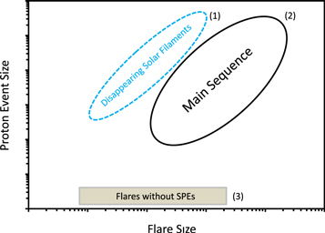
In Figure 17 we present a schematic, patterned after Figure 15, that characterizes our view of the general relationship between SPE and flare size parameters in large, well-connected prompt SEP events. This view is based on comparisons of SEP parameters versus gamma-ray line emission (Cliver et al. 1989), SXR emission (Cliver et al. 2012; Laurenza et al. 2018), 1 MHz radio emission (Cliver & Ling 2009; Laurenza et al. 2018), 35 GHz radio fluence (Grechnev et al. 2015), and reconnection flux (Kahler et al. 2017), covering a range of SEP energies from >10 to >100 MeV. There are three main zones or regions in the diagram:
- (1)DSFs with associated SPEs. This region indicates that large flares are not a necessary condition for a large SEP event. This is the least populated zone in the schematic because DSFs generally may be thought of as "soft" low-energy two-ribbon flares (Kiepenheuer 1964) and thus are less likely to have high-speed CMEs that can drive shocks. That said, the assessment of Klein & Dalla (2017) that "whatever the interpretation of the filament-associated SEP events, there are at best very few SEP events associated with a CME and no alternative signature of particle acceleration in the corona" misses the point about the importance of anomalies (e.g., Sturrock 2017). Also, the characterization by Belov (2017; quoted in Section 1) that such SPEs either originate in sources behind the Sun's western limb, for which the flare source is occulted, or are small proton events occurring on a high SXR background that masks the flare source does not hold for the 2013 September 29 event (Figures 1–3) and the other events in Table 2. We note that the separation of the ("weak flare/strong SPE") region from the main sequence (i.e., zone (1) from zone (2)) in Figure 17 is for illustrative purposes only—to highlight the importance of DSF-associated SPEs for our understanding of SEP acceleration. It is not meant to imply a difference in the primary mechanism of SEP acceleration (CME-driven shocks) operating in this zone and on the main sequence, although the details of this process (see Section 3.2.2) may have a quasi-systematic variation. Nor do we expect a sharp demarcation of SEP properties between zones 1 and 2, but rather a gradient as observed for the Fe/O ratio in Figure 15.
- (2)The main sequence, large flares with SPEs. The general correlation of SEP and flare parameters on the main sequence is attributed to the big flare syndrome (Kahler 1982). Big flares tend to have more of everything, so such high-scatter correlations are inescapable in comparisons of flare and SEP parameters. The main sequence is a key reason for the resilience of the view that a flare-resident acceleration process plays an important role in proton acceleration at the Sun, particularly at higher energies (e.g., Dierckxsens et al. 2015; Grechnev et al. 2015). In Dierckxsens et al. (2015) and Trottet et al. (2015), as well as Cliver et al. (2012), the authors considered a list of SEP events and their associated flares, not taking into account comparable flares (in the parameter considered) that lacked such SEP association. Figures 4 (adapted from Kahler et al. 2017) and 9 (after Grechnev et al. 2015)—which both take non-SEP flares into account—show how ignoring flares without associated SEPs overstates the SEP versus flare correlation.
- (3)Flares without associated SPEs (only background SEP intensities). This region indicates that large flares are not a sufficient condition for a large SEP event. For the reconnection flux (Figure 4), this is the most populated zone of the diagram, while there are relatively few gamma-ray line flares that lack associated SPEs (see Figure 2 in Cliver et al. 1989). This difference is a reflection of the big flare syndrome—larger, more energetic flares such as gamma-ray flares are more likely to have associated fast CMEs, shocks, and therefore SEPs. In comparison, only half (36/72) of the reconnection flux events in Table 1 had associated CMEs. This zone of events consists of two subclasses: (1) flares without CMEs and (2) flares with relatively slow (median speed ~400 kms-1) CMEs. Both conditions argue against shock acceleration of SEPs (see, e.g., Figure 2 in Cliver & D'Huys 2018).
Figure 17. Schematic comparison of SPE vs. flare size parameters for large, well-connected SPEs showing three characteristic zones of events: (1) DSF-associated SPEs, (2) main sequence of SPEs associated with big flares and strong shocks, and (3) non-SPE events with either no or slow associated CMEs.
Download figure:
Standard image High-resolution image
As zones 3 and 1 of Figure 17 show, respectively, big flares can lack SEP association and some weak flares can be associated with large SPEs. Taking both of these regions into account weakens SEP versus flare correlations (e.g., Figures 4 and 9). In addition, zone 1 underscores the prevailing view that fast CMEs and the shocks they drive are the principal requirements for large SEP events.
We are not saying that protons are not accelerated in impulsive flares (or during the impulsive phase of fully developed flares). They clearly are, including to high energies (see, e.g., Forrest & Chupp 1983; Forrest et al. 1985; Chupp et al. 1987; Ackermann et al. 2012). Also, it has long been known that type III radio bursts, the characteristic emission of the flare impulsive phase (Wild et al. 1963), are associated with electron-rich (Lin 1970) and 3He-rich events (Reames et al. 1985) at 1 au—so particles can escape from flares. Such SPEs will populate parameter space below zones 1 and 2 and above zone 3 in Figure 17 (as in, e.g., Figure 11 in Cane et al. 2010). What is lacking at this point, however, is compelling evidence that flares, either during their classic impulsive phase or in the extended phase of type III emission first identified by Cane et al. (1981), are able to make a significant, let alone dominant, contribution to large (gradual) proton events. The principal problem is the proton deficiency of flare-accelerated particles. The electron-to-proton ratios (for both (0.5 MeV electrons/>10 MeV protons) and (0.5 MeV electrons/>100 MeV protons)) of the largest impulsive SEP events are approximately two orders of magnitude larger than those of the largest gradual SPEs (Cliver & Ling 2007; Cliver 2016). It is not possible to produce a large SPE by scaling up a classic impulsive SPE without giving rise to electron events much larger than observed to date. For the extended or delayed 1 MHz emission, termed type III-l by Cane et al. (2002), Cliver & Ling (2009) showed that the median >30 MeV proton yield for a sample of large proton events was ∼280 times larger than that for classic impulsive events and concluded that the greater proton yield of the gradual events was due to the fact that such events are strongly associated with DH type II shocks, in contrast to large impulsive SPEs.
Cane et al. (2010) criticized the Cliver & Ling (2009) analysis, writing, "(1) ... Cliver & Ling (2009) failed to take account of the timing of the type III emission relative to the flare emissions. (2) Their comparison of radio intensities and proton intensities takes no account of the fact that they compare inferred total electron intensities relatively close to the Sun with observations at 1 au, where only a part of the particle beam would be intercepted." Regarding item 1, Cane et al. are correct that Cliver & Ling combined the impulsive and delayed type III emission for gradual events, but excising the impulsive phase type IIIs to isolate the delayed emission would only make the proton yield larger for gradual SPEs, further distinguishing them from the low-yield impulsive SPEs. Regarding item 2, what Cliver & Ling (2009) did in their Figure 6 (a scatter plot of proton intensity vs. 1 MHz fluence) is no different conceptually than what Cane et al. (2010) did in their Figure 11 (a scatter plot of proton intensity vs. SXR intensity). In fact, the assumption both studies followed—that flare electromagnetic emissions are (or could be) representative of SPE size parameters at Earth—underlies all such flare–SPE comparisons. One cannot rule out the possibility that the late-phase type III bursts associated with large (≥10 pfu at >10 MeV) SPEs are a signature of a nonshock acceleration process that produces SPEs with substantially different composition and higher proton yields than those associated with impulsive phase type IIIs, but this remains to be proven.
3.2.2. SPE Spectra and Fe/O Ratios and CME Acceleration
Gopalswamy et al. (2015, 2016, 2017a) have recently reported that, on average, the CMEs associated with DSFs have lower initial acceleration rates (leading to greater heights of shock formation and lower type II starting frequencies) than the eruptions associated with GLEs. This linkage of shock and SPE properties counters the argument of Grechnev et al. (2015) that the soft SEP spectra of "non-flare-related-SPEs" weighs against the capability of shocks to accelerate protons to high energies on the main sequence. More directly, the consensus of several recent analyses of late-phase solar gamma-ray events that are associated with main-sequence flares (median SXR class of X1.1; Table 1 in Share et al. 2018) is that CME-driven shocks are capable of accelerating protons to the highest energies (≳300 MeV) that can be inferred from gamma-ray observations (e.g., Pesce-Rollins et al. 2015; Ackermann et al. 2017; Plotnikov et al. 2017; Gopalswamy et al. 2018; Kahler et al. 2018; Jin et al. 2018; Omodei et al. 2018; Winter et al. 2018; c.f., Grechnev et al. 2018; Hudson 2018; Klein et al. 2018).
The hierarchal view of SEP acceleration of Gopalswamy et al. (2016, 2017a), viz., the correlation of initial CME speeds (i.e., early acceleration rates) and SPE spectra, had a precursor in the Nitta et al. (2003a) study that suggested differences in SPE spectra/composition/charge state between eruptive flares exhibiting explosive and gradual (during an extended pre-eruption phase) outward motions. The hierarchal picture can be seen as being complementary to the Tylka et al. (2005) shock formulation if quasi-perpendicular shocks are most effective low in the corona where the CME expands laterally, and quasi-parallel shocks dominate above the nominal ∼2 R⊙ maximum height of closed loops. The analytical model of Tylka & Lee (2006) incorporated shock geometry and seed particle populations to provide an explanation of the event-to-event variation of elemental composition at high energies first noted by Breneman & Stone (1985). In this model, SPEs with high Fe/O ratios are attributed to quasi-perpendicular shock acceleration of flare suprathermals (c.f., Mewaldt et al. 2007, 2012) and events with low Fe/O ratios to quasi-parallel shock acceleration of coronal or solar wind suprathermals. If the predominantly low Fe/O ratios of DSF- and quasi-DSF-associated SPEs in Table 2 indicate quasi-parallel shock acceleration, then the near-even mixture of the number of SPEs with high and low Fe/O ratios (17 and 15, respectively) in the black oval in Table 15 implies a greater role for quasi-perpendicular shock acceleration on the main sequence.
3.2.3. Predictions and Understanding
A key test of understanding of SEP acceleration at the Sun is the ability to issue reliable alerts of impending SEP events based on observations of eruptive flares. Consideration of the DSF-associated SPE of 2013 September 29 in the proton alert study of Laurenza et al. (2018) indicates that attempts to understand large SPEs in terms of a flare-resident acceleration process, using flare diagnostics (Figure 16), are off track. The flare parameters for the 2013 September 29 DSF are an order of magnitude too small to provide an alert without an unacceptably high false-alarm rate. While flare-based alert methods such as ESPERTA have a demonstrated utility for timely warnings, significant advances in SEP forecasting require a focus on fast CMEs and shocks. Recent studies by St. Cyr et al. (2017) and Richardson et al. (2018) have placed more emphasis on these phenomena.
S.K. was supported by AFOSR Task 18RVCOR122. M.D.K. acknowledges support from the National Science Foundation, SHINE, AGS 1622495. This work was in part carried out on the open-use data analysis computer system at the Astronomy Data Center (ADC) of the National Astronomical Observatory of Japan. M.S. was supported by JSPS KAKENHI grant No. JP17K05397. The LASCO CME catalog used in this study is generated and maintained at the CDAW Data Center by NASA and the Catholic University of America in cooperation with the Naval Research Laboratory. SOHO is a project of international cooperation between ESA and NASA. E.W.C. has benefited from participation on the ISSI International Team led by Athanasios Papaioannou, which is investigating high-energy solar particle events. We thank an anonymous referee for a detailed and helpful review of this work.
Footnotes
- 7
- 8
For C-class SXR flares the peak intensity is (1–9) × 10−6 W m−2 (for B-class/M-class/X-class flares, the exponent is −7/−5/−4).
- 9
For the definition of the National Oceanic and Atmospheric Administration (NOAA) S1−S5 radiation scales, see http://www.swpc.noaa.gov/noaa-scales-explanation.
- 10
The nominal DH range of 14–1 MHz is that covered by the RAD2 instrument on Wind Waves. The 14 MHz frequency corresponds to the plasma frequency at ∼3 R⊙, and frequencies of 1–2 MHz correspond to ∼10 R⊙ (Cliver et al. 2004; Gopalswamy et al. 2015). DH type II archives: https://cdaw.gsfc.nasa.gov/CME_list/radio/waves_type2.html; https://solar-radio.gsfc.nasa.gov/wind/dataproducts.html).
- 11
Archive for metric bursts: https://www.ngdc.noaa.gov/stp/space-weather/solar-data/solar-features/solar-radio/radio-bursts/reports/spectral-listings/ (for 1967–2010); ftp://ftp.swpc.noaa.gov/pub/warehouse/2011/2011_events.tar.gz for subsequent years, replacing 2011/2011 with 2012/2012, etc.
- 12
Following Grechnev et al. (2015), we omitted the 1991 May 18 data point (1.43E+7; 4.34E+3).
- 13
Because ESPERTA is designed to provide alerts within 10 minutes of SXR maximum, the plotted data points in Figure 16 (including the three in Figure 16 highlighted by black circles) are based on real-time algorithm-based estimates of the 1–8 Å and 1 MHz fluence rather than the actual values given in Table 2. The open red squares in Figure 16 are based on the Table 2 values. In most cases, as holds for the Table 2 events, the algorithm-based estimates are within a factor of two of the actual values of the SXR and 1 MHz fluences.