


Abstract
The impact of the nonstationarity of the heliospheric termination shock in the presence of pickup ions (PUIs) on the energy partition between different plasma components is analyzed self-consistently by using a one-dimensional particle-in-cell simulation code. Solar wind ions (SWIs) and PUIs are introduced as Maxwellian and shell distributions, respectively. For a fixed time, (a) with a percentage of 25% PUIs, a large part of the downstream thermal pressure is carried by reflected PUIs, in agreement with previous hybrid simulations; (b) the total downstream distribution includes three main components: (i) a low-energy component dominated by directly transmitted (DT) SWIs, (ii) a high-energy component dominated by reflected PUIs, and (iii) an intermediate-energy component dominated by reflected SWIs and DT PUIs. Moreover, results show that the front nonstationarity (self-reformation) persists even in presence of 25% PUIs, and has some impacts on both SWIs and PUIs: (a) the rate of reflected ions suffers some time fluctuations for both SWIs and PUIs; (b) the relative percentage of downstream thermal pressure transfered to PUIs and SWIs also suffers some time fluctuations, but depends on the relative distance from the front; (c) the three components within the total downstream heliosheath distribution persist in time, but the contribution of the ion subpopulations to the low- and intermediate-energy components are redistributed by the front nonstationarity. Our results allow clarifying the respective roles of SWIs and PUIs as a viable production source of energetic neutral atoms and are compared with previous results.
Export citation and abstract BibTeX RIS
1. Introduction
The heliospheric termination shock (TS) is the transition layer between the supersonic solar wind and the subsonic heliosheath of the solar material in the interstellar medium (Burlaga et al. 2005; Decker et al. 2005; Jokipii 2008; Richardson et al. 2008). Voyager 1 (V1) and 2 (V2) crossed the TS in 2004 December at a distance of about 94 au (Stone et al. 2005) and in 2007 August at about 84 au, respectively (Decker et al. 2008). Both Voyager spacecraft have provided magnetic field data during the TS crossings, and the in situ observations show that the spacecraft suffered multiple crossings instead of the single crossing expected at the shock (Burlaga et al. 2008). Such multiple crossings may be due to a nonstationarity of the shock front, in particular the self-reformation process driven by the accumulation of reflected-gyrating ions in the "foot" region just ahead of the shock "ramp" region (see Lembege & Dawson 1987, and Lembege & Savoini 1992 for studies of reformation with no pickup ions (PUIs)). From the plasma measurements, it was concluded that the solar wind cool ions account for about 15% of the dissipation at the TS (Richardson et al. 2008). It is generally believed that the interstellar-origin PUIs (Vasyliunas & Siscoe 1976) dominate the plasma dissipation process across the TS, which has been predicted with modeling (Zank et al. 1996, 2010), and verified quantitatively with hybrid simulations (Wu et al. 2009, 2010) and with PIC simulations (Matsukiyo & Scholer 2011, 2014; Oka et al. 2011; Yang et al. 2013, 2014, 2015; Lembege et al. 2014). On the other hand, the relative efficiency of acceleration mechanisms (SDA as shock drift acceleration and SSA as shock surfing acceleration) has been analyzed in simulations where PUIs are introduced as test particles with a shell distribution (Yang et al. 2009; Burrows et al. 2010). However, the test-particle approach is not appropriate when PUIs are non-negligible. In fact, Lembege & Yang (2016) have analyzed the impact of a substantial amount of PUIs on the microstructures of the shock front. It remains unclear, however, precisely how a substantial amount of PUIs ultimately affects the energy partition of different ion components. Moreover, the impact of the nonstationary shock front on the particle velocity distributions in the downstream/heliosheath region should be further investigated.
More than two decades ago, Liewer et al. (1993) have investigated the impact of PUIs on the shock microstructures with a hybrid code. They found that an extended foot appears to be associated with some reflected PUIs. Kucharek & Scholer (1995) have also performed hybrid simulations of PUI loaded shocks and have focused on the impact of the shock normal angle on the PUIs escape from the shock front. These PUIs are thought to take part in a diffusive acceleration process. Lipatov & Zank (1999) have simulated shocks with PUIs with a hybrid simulation code that included a finite electron mass fluid. They reported that PUIs gain energy through multiple reflections by the cross-shock potential with a sufficiently small thickness, i.e., shock surfing acceleration mechanism (Lee et al. 1996; Zank et al. 1996; Shapiro & Ücer 2003). Nevertheless, Lipatov & Zank (1999) also pointed out that the different artificial resistivity employed in the hybrid model can lead to different shock front widths, cross-shock potential, and particle dissipation processes.
Full particle simulations of a shock with 10% relative PUI density upstream have been first performed more than 10 years ago (Chapman et al. 2005; Lee et al. 2005). Based on 1D PIC simulations of a strictly perpendicular shock, the authors also obtained an extended foot, as in previous hybrid simulations, and analyzed the cross-shock electric field based on a two-fluid model. Scholer et al. (2003) concluded that even without PUIs, the cross-shock potential is not strong enough for an efficient shock surfing/multiple reflection acceleration of PUIs. Matsukiyo et al. (2007) have studied the modified two-stream instability (MTSI) triggered within the foot of an oblique (quasi-perpendicular) shock in the presence of PUIs, and have shown that the MTSI is responsible for the self-reformation of the shock front even in the presence of PUIs. They emphasized the importance of using a realistic ratio of ion to electron mass in the PIC simulations. Indeed, the use of a mass ratio lower than 400 may suppress the excitation of the MTSI in the foot of the shock. Using a real mass ratio (i.e., mi/me = 1836), Yang et al. (2012) investigated the contributions of different terms in the generalized Ohm law to the cross-shock electric field/potential for a strictly perpendicular shock. The authors concluded that in the low PUI% case, the supercritical shock front is nonstationary and self-reforming, as in Lembege & Dawson (1987) and Hada et al. (2003); there is an interplay between the contributions of the Lorentz and Hall terms and the cross-shock electric field. In the foot-growing phase, the Lorentz term always dominates the extended PUI foot region; the Hall term competes with the Lorentz term within the foot of solar wind ions (SWIs), and the Hall term supported by the SWIs becomes very important at the steepened ramp of the shock. In the high PUI% case (55%), the SWI foot almost disappears and the shock front becomes quasi-stationary, as analyzed also by Lembege & Yang (2016). Yang et al. (2015) found that the extended foot (mainly controlled by PUIs) is dominated by the Lorentz force, while the ramp is mainly dominated by the Hall term supported by the SWIs. Lembege & Yang (2016) have emphasized that the stationarity/nonstationarity of the shock front is mainly controlled by the relative strength of the Mach regime (high MA is in favor of front nonstationarity) versus the percentage of PUIs (high PUI% is in favor of front stationarity). This competition can be expressed in terms of need for local dissipation at the ramp. Without any foot structure, the ramp has to evacuate the extra energy (in the high Mach regime) by reflecting a part of the incoming ions as these directly reach the ramp. A foot structure forms ahead of the ramp, and the local need for dissipation at the ramp decreases, since the bulk motion of the incoming plasma is reduced through the foot. If a multi-scale foot forms (as in the present case, with a PUI and SWI foot), the local need for dissipation at the ramp is even lower. In high PUI%, the extended PUI foot strongly brakes down the bulk motion of the incoming plasma over a large upstream region before it reaches the ramp, and the local need for dissipation at the narrow ramp is quite reduced. The SWI foot that controls the front self-reformation almost disappears and the whole front becomes stationary.
The time-evolving microstructures of the TS and particle dynamics in the presence of PUIs with different percentages of PUIs, different thickness of the upstream shell distributions describing the PUIs for different Mach regimes, and the impact of the shock front self-reformation have been analyzed with a 1D PIC simulation (Yang et al. 2013, 2014; Lembege et al. 2014). In particular, results have shown that in absence of PUIs, the PUI and SWI bulk dynamic energy is transferred to the thermal energy of SWIs; in contrast, in the presence of 25% PUIs, most upstream dynamic energy is transfered through the shock front to the PUIs instead of the SWIs. A detailed analysis of the time-dependent shock-front microstuctures has been performed and summarized in Lembege & Yang (2016). We recall two important points: (i) previous hybrid simulations including PUIs did not involve any shock front nonstationarity (such as the self-reformation), which requires a high spatial resolution where the grid size Δ is least Δ < 0.5 c/ωpi , as shown by Hellinger et al. (2002) in absence of PUIs; (ii) the shock front self-reformation analyzed herein (and in Lembege & Yang 2016) is based on the accumulation of reflected SWIs over a foot distance from the ramp. This self-reformation persists for an oblique (quasi-perpendicular) shock in 1D and 2D simulations (Lembege & Savoini 1992; Lembege et al. 2004), but differs from the one analyzed by Matsukiyo et al. (2007) that is based on MTSI, which requires an oblique shock propagation and a relatively high mass ratio above a certain threshold (Scholer & Matsukiyo 2004).
Moreover, 2D PIC simulations (Yang et al. 2015) have been performed in conditions identical to those previously used in 1D PIC for a strictly perpendicular shock (Yang et al. 2013, 2014; Lembege et al. 2014) and recovered same results both in terms of shock structure and dynamics, and of energy partition obtained along the shock normal. This suggests that 2D effects do not bring major changes with respect to the 1D results (along the normal to the shock front), although the impact of 2D effects has not been analyzed in detail; at this stage, 2D results indicate that the downstream pressure of PUIs can vary from 61.9% to 96.3% in the direction perpendicular to the shock normal due to the front ripples. These results by Yang et al. (2015) may shed light on the properties of the PUIs at the TS, while the less energetic, solar wind core component was directly studied with the Faraday Cup instrument on board V2.
The present paper is an extension of Lembege & Yang (2016; named herein Paper 1), is mainly focused on the energy partition between the different plasma components, and analyzes how the nonstationarity of the shock front impacts the downstream energy partition and particle velocity distribution, and vice versa. With the help of an automatic separation method (ASM, as in Yang et al. 2009 and in paper 1), which is inspired by the previous work of Burgess et al. (1989) that was based on hybrid simulations, we analyze separately this impact on reflected (R) and directly transmitted (DT) ions for both SWI and PUI populations. In summary, the main questions addressed in this paper are (1) the quantitative profiles of the energy partition across the shock, i.e., within the foot, ramp, immediate, and far downstream regions of the TS, where the TS microstructures are self-consistently included in all SWI, PUI, and electron scales; (2) the resulting energy spectra (spatially integrated), (3) the time-evolving individual contributions of R and DT ions to the velocity distribution of PUIs, SWIs, and the total ion distribution Fi,tot measured downstream of the TS, and (4) the effect of the self-reformation of the shock front on the downstream plasma pressure, bulk speed, and density profiles, which can be used as inputs in further global magnetohydrodynamics (MHD) simulation models of the heliosphere.
The paper is organized as follows. Section 2 summarizes the conditions of numerical simulations. Section 3 presents a detailed analysis of local ion distributions at/around the shock front and far downstream, which emphasizes the necessity for considering R and DT ions separately for SWIs and PUIs. Section 4 analyzes the impact of the shock front nonstationarity on the ion reflection rate for each population, and on the energy partition between the different ion subpopulations (R–SWIs, DT–SWIs, R–PUIs, and DT–PUIs) from upstream to downstream regions; in addition, this impact is also analyzed in detail on the downstream heliosheath distribution and on its contributing subpopulations, and results are compared with models proposed in previous works. Discussion and conclusions are presented in Section 5.
2. Numerical Simulation Conditions
In order to answer the questions listed above, we use a 1D electromagnetic PIC code in conditions identical to those of Paper 1; the x-coordinate is defined along the spatial axis of the box. Three species are included in the simulation: the electrons (el), the SWIs, and the PUIs. Since our topics are focused on energy partition, we have verified that the total energy (including all fields and particle species) in the simulation box is well conserved (within 5%) in a thermal run (no shock). The shock is produced by the injection method, as in previous works (Lee et al. 2005; Matsukiyo et al. 2007; Lembege et al. 2014; Yang et al. 2013, 2014). All particles are injected on the left-hand side of the simulation box with an inflow/upstream drift speed Vinj, and are reflected at the other side (reflecting wall). The distribution functions for the SWIs and electrons are Maxwellian, while PUIs are injected into a sphere in velocity space centered at Vinj with radius Vshell, as in earlier works (Lee et al. 2005; Matsukiyo & Scholer 2011). Paper 1 has shown that the thickness of the shell has no noticeable impact on the microstructures on the shock front and on its time dynamics. Then, we use a zero-thickness shell for simplicity, which will allow us to compare our results here with the results obtained in previous works and in Paper 1. The shock builds up and moves with a speed Vref from the right-hand to the left-hand side. The upstream Alfvénic Mach number of the shock is MA = (Vinj + Vref)/VA, where the Alfvén velocity VA is equal to 1. The ambient magnetostatic field along the y-direction is ∣Bo∣ = 1. All upstream plasma parameters are summarized in Table 1. Our study here is based on three simulation runs (Table 2), as in Paper 1, corresponding to three different percentages of PUI% = 0, 10, and 25, respectively, with supercritical Alfvén Mach number of MA = 4.78, 4.99, and 5.26. The plasma box size length Lx = 80 c/ωpi (where c/ωpi is the upstream ion inertia length) for the different Mach number cases; the velocity of light c = 20, the mass ratio mi/me = 100, and the ratio of electron plasma to cyclotron frequency ωpe/Ωce = 2. The SWI beta βi = 0.04, which is inferred from Voyager data for TS-3 (Burlaga et al. 2008). Electron beta βe = 0.5 is chosen as in previous PIC simulations (Lee et al. 2005). Initially, there are 200 particles of each species in a cell. The upstream plasma is quasi-neutral, i.e., ne = ni , where ni = nSWI + nPUI = NSWI ∗ SWI% + NPUI ∗ PUI%, where ne, ni, nSWI, and nPUI are densities of electrons, of total ions, of SWIs, and of PUIs, respectively; and NSWI, NPUI, and SWI%, and PUI% are the counts of each species of ions and their relative weighted percentage in the PIC simulation, respectively.
Table 1. Plasma Parameter Values Used in the Simulations
| Parameter | Description | Electrons | SWIs | PUIs |
|---|---|---|---|---|
| vth | Thermal velocity | 7.07 | 0.2 | Shell distribution |
| λD | Debye length | 0.035 | 0.0071 | |
| ρc | Gyro-radius | 0.0707 | 0.2 | |
| c/ωp | Inertial length | 0.1 | 1 | |
| ωc | Gyro-frequency | 100 | 1 | |
| ωp | Plasma frequency | 200 | 20 | |
| τc | Gyro-period | 0.01 | 1 | |
| β | Plasma beta | 0.5 | 0.04 |
Download table as: ASCIITypeset image
Table 2. Main Plasma Parameters and Shock Conditions Measured in the Different 1D PIC Simulation Runs; Tref is the Time Period of the Cyclic Self-reformation
| PUI% | Vinj | MA |

|
|
|---|---|---|---|---|
| Run 1 | 0 | 3 | 4.78 | 1.729 |
| Run 2 | 10 | 3 | 4.99 | 1.539 |
| Run 3 | 25 | 3 | 5.26 | 1.401 |
Download table as: ASCIITypeset image
3. Local Ion Distributions Measured at/around the Shock Front
A typical shock profile is shown in Figure 1 for PUI% = 10, with the associated phase space of SWIs and PUIs at a fixed time of the run. For each population, incident ions are separated into reflected (label R with red dots) and directly transmitted (label DT with black dots) parts using the ASM (the method is described in Paper 1). Here, we can identify various spatial structures in Figure 1: (a) an extended PUI foot, (b) an SWI foot with smaller width, (c) a very narrow ramp, and (d) a first (O1) and a second (O2) overshoot mainly supported by the gyrating DT–SWIs in the downstream region. Moreover, Figure 2 summarizes complementary information on the front dynamics: (i) the self-reformation of the shock front persists even for a substantial percentage of PUIs (25%) because the Mach number regime is sufficiently high (MA = 5); (ii) this self-reformation leads to large field fluctuations at the front (overshoot O1) and farther downstream (the fluctuations of O2 are more reduced than those of O1); (iii) the spatial widths of the microstructures (the PUI foot, the SWI foot, and the distance LO1–O2 between overshoots "O1" and "O2") fluctuate with a time period equal to the self-reformation cycle; in contrast, the ramp width is not affected by the self-reformation and stays unchanged for the different PUI% runs; (iv) as the PUI% increases, the amplitude of the field fluctuations (O1 and O2) is reduced while the amplitude of the PUI foot increases; and (v) the time-averaged distance  increases with PUI%. In summary, the front width progressively increases from a relatively narrow profile that includes the SWI foot, the ramp, and the overshoot O1 (for PUI% = 0), to a very extended profile starting from the upstream edge of the PUI foot to—at least—the downstream overshoot O2 (for PUI% = 25). This means that we need to carefully analyze the impact of both PUI% and the front nonstationarity on the energy partition at different locations throughout the front: at/around the front itself, and farther downstream.
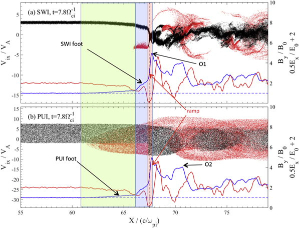
Figure 1. Phase space plots (xi–vxi) of the (a) solar wind ions (SWIs) and (b) pickup ions (PUIs) at the shock in the presence of 10% PUIs at time t = 7.8  . The upstream incident ions are separated into two parts at the shock front: reflected (red dots) and directly transmitted ions (black dots). In each panel, the zoomed and shifted magnetic field By (blue curve) and cross-shock electric field Ex (red curve) are shown for reference. The PUI foot, SWI foot, and ramp regions are highlighted in green, blue, and red, respectively. The vertical dashed line indicates the ramp location (x = 67.5 c/ωpi) where the amplitude of the field Elx is maximum. Overshoots "O1" and "O2" are marked by the black arrows.
Download figure:
Standard image High-resolution image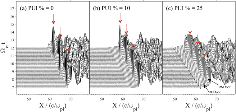
Figure 2. Time stackplot of the main magnetic field By, for three simulations performed at various relative percentages of PUI% = 0 (run 1), 10 (run 2), and 25 (run 3). All simulations are conducted at MA = 4.78, 4.99, and 5.26. In each panel, three successive overshoots "O1" (related to SWIs) are marked by red arrows. The dashed line in panel (c) shows the leading edge of the PUI foot.
Download figure:
Standard image High-resolution imagePhase spaces of the different ion populations are shown for the different PUI% (=0, 10, and 25) in Figure 3, where the Btz and Elx field components are reported for reference. Red and black dots denote the DT and R ions, respectively, for each population. While Figure 3 already indicates that PUIs are reflected more efficiently than SWIs (as we confirm in Section 4), we first discuss the corresponding energy gain below. Note also that as explained in Paper I, the shock front velocity increases as the PUI% increases, as indicated by the different locations of the shock front (the thick dashed line) in the different panels of Figure 3, while the amplitude (overshoot "O1") decreases.

Figure 3. Phase space plots of SWIs (panels a–c) and PUIs (panels d–f) at the same fixed time t = 7.8  , for different percentages of PUI% = 0 (run 1), 10 (run 2), and 25 (run 3), where the Mach number equals MA = 4.78, 4.99, and 5.26, respectively. For each population, reflected (R) and directly transmitted (DT) ions are represented by red and black dots. In each panel, the zoomed and shifted field components By (blue curve) and Ex (red curve) are shown for reference. The vertical dashed line indicates the ramp location where the amplitude of the field Ex is maximum. For PUI% = 25, the vertical arrow "O" indicates the location of the old ramp of the previous self-reformation; "O1" denotes the first overshoot.
Download figure:
Standard image High-resolution imageThe impact of different PUI% on the local ion distribution measured around the shock front for each population is illustrated at a fixed time ( ) for SWIs and for PUIs in Figures 4(a) and (b), respectively. In each figure, the top and bottom panels correspond to measurements made within a spatial range Δxsamp = 10 c/ωpi defined upstream and downstream from the ramp location, respectively (indicated in Figure 3 by a vertical dashed line where the amplitude of Ex field is maximum, and where the Btz field profile presents an inflection point). We use test particles for the statistics of PUIs in the case PUI% = 0, and red and dark dots are used for the statistics of R and DT ions for each ion population. In all cases, the main results for Figure 4(a) (SWIs) are summarized as follows: (i) the upstream distribution includes the unchanged incoming SWIs and a small bump at lower bulk velocity, which illustrates that SWIs are slowed down by the R–PUIs upstream before they reach the ramp (as in Kucharek et al. 2010); this slowdown is also clearly apparent in the SWI phase space of Figure 3); (ii) as expected, both R–SWIs and DT–SWIs gain high energy when moving from upstream (top panels) to downstream (bottom panels) correspondingly for each case; (iii) for all PUI% cases, the gain of energy downstream is higher for R ions than for DT ions (bottom panels); (iv) a relatively narrow beam is always observed in the upstream R–SWIs; its features vary in the different PUI% cases, but no clear conclusions (in terms of Vxi bulk velocity and temperature) versus PUI% can be reached since they are impacted in time by the self-reformation itself; (v) the maximum downstream energy range (bottom panels) for R–SWIs (deduced by the width of each distribution) decreases as PUI% increases: the velocity interval is Δ(vxi/VA) = (−8, 7) and (−5.5, 5) for PUI% = 0 and 25), respectively; in contrast, the width of the downstream DT–SWI distribution is almost independent of the PUI% (Δ(vxi/VA) = (−4, 4)); (vi) the R–SWI downstream distribution approaches a flat-top shape for higher PUI% (=25), which suggests a strong contribution of the Elx field (when invoking the similarity with electron distribution function measured at similar locations throughout the front (Savoini & Lembege 1994)); and (vii) the most energetic SWIs observed downstream correspond to the "old" R–SWIs that have suffered a few gyrations after these succeeded in penetrating the downstream region (over the distance Δxsamp = 10 c/ωpi; see the red dots in Figure 3).

Figure 4. Local ion distributions Fi (vxi) measured at the same fixed time t = 7.8  around the shock front within the upstream (US) spatial range Δx = −10 c/ωpi (upper panels) and the downstream (DS) spatial range Δx = +10 c/ωpi (bottom panels), respectively; these ranges are defined based on the ramp location xramp, as illustrated by two two-way arrows at the top of Figure 3(d). Within each plot, the red and black circles correspond to the reflected (R) and directly transmitted (DT) ions, respectively. Figures 4(a) and (b) correspond to measurements performed for SWIs and PUIs, respectively. For each panel, the plots correspond to different percentages of PUI% = 0 (run 1), 10 (run 2), and 25 (run 3). The case where PUI% = 0 (the PUIs are introduced as test particles) is shown in plots (i) and (iv) of Figures 4(a) and (b) for reference.
Download figure:
Standard image High-resolution imageFigure 4(b) presents the PUI velocity distributions in the same spatial ranges with the same format as Figure 4(a). The main results are as follows: (i) since the region occupied by the PUIs is more extended upstream than that covered by SWIs (Figure 1), the differences between upstream and downstream distributions are less drastic for PUIs than for SWIs; (ii) the upstream R–PUI distribution approaches a flat-top shape superimposed by a beam with a negative bulk velocity centered around Vxi = 2.5–3 VA), which is almost unchanged for different PUI%; (iii) in contrast with SWIs, the downstream R–PUI distribution (bottom panels) takes a clear flat-top shape for all PUI cases; the distribution becomes narrower with a decrease in the maximum velocity range of the distribution from 12.0, 11.5, and 11.0 for PUI% = 0, 10, and 25; (iv) the downstream DT–PUI distribution presents a similar flat-top regardless of the PUI%, but the most energetic PUIs correspond to the "old" R–PUIs, i.e., those that have succeeded in reaching the downstream region where they only suffered one large gyromotion (see the red dots representing the R–PUIs within the range Δxsamp = 10 c/ωpi in Figure 3).
In summary, a comparison between Figures 4(a) and (b) clearly shows that the maximum velocity range of PUIs is always larger than that of SWIs, and the most energetic downstream ions (bottom panels) are the R–PUIs, regardless of the PUI%. One large gyromotion is enough for PUIs to play a key role. These results are quite helpful for modeling upstream/downstream ion distribution functions, for which the contributions of R and DT ions are needed to be identified separately for SWI and PUI populations, and to analyze their possible impact as sources of energetic neutral atoms (ENAs), as discussed in Section 5.
4. Impact of the Front Nonstationarity on PUIs and SWIs
4.1. Impact on the Percentages of the Reflected PUI and SWI Density
An illustration of the impact of the self-reformation on each population is given in Figure 5, which represents the variation in percentage of reflected ions (R%) within a time range covering more than two self-reformation cyclic periods. Our previous paper 1 has only indicated the time-averaged value of R%, but not the variation in R% versus time; here, the counting of reflected ions is similar to that used in Paper 1. For the case PUI% = 0, where PUIs are absent, statistics are again performed with test particles describing the PUIs. The main results are that (i) the time-averaged value of R% is always higher for PUIs than for SWIs, regardless of the PUI%, (ii) the time variation in R% is relatively weak (a few %) for both PUIs and SWIs, and (iii) as the PUI% increases, the time-averaged value of R% decreases for both PUIs and SWIs, and the amplitude of the R% variation becomes smoother. The fact that R% decreases for both PUIs and SWIs is a direct consequence of the time-averaged field amplitude decrease at the shock front as the PUI% increases, and more SWIs and PUIs are DT (Paper 1). Then, a noticeable impact on the local downstream ion distribution and on the global energy partition is expected, as shown in the next sections.
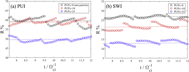
Figure 5. Time history of the percentage of reflected PUIs (panel a) and SWIs (panel b). This percentage is measured in the downstream region (within a sampling interval Δxsamp = (xramp, xramp + 10 c/ωpi) measured from the location xramp of the shock ramp identified at each time). Each panel includes measurements performed for the three different percentages of PUI% = 0 (dark dots), 10 (red dots), and 25 (blue dots) and covers more than two cyclic self-reformations periods. The case where PUIs = 0% (the PUIs are introduced as test particles) is shown as a reference. The horizontal dashed colored lines represent the time-averaged value corresponding to each case.
Download figure:
Standard image High-resolution imagePaper 1 has shown that the reflection rate of SWIs (i.e., the ratio NR_SWIs/NSWIs of reflected SWIs density over the total density of incident SWIs) strongly decreases from 24.78%, to 16.81%, and 8.95%, as the PUI% increases from 0 to 10 and 25, i.e., for runs 1 to 3, respectively. In contrast, the reflection rate of PUIs very slightly decreases to 47.82% (test particles), to 47.77% and 47.44% as the PUI% increases from 0 (test particles) to 10 and 25 (TS conditions), i.e., for runs 1 to 3, respectively. Note that the reflection rate is based on the separation method described in Section 1. In short, we start counting the R ions and DT ions from a given time tA (= 7  ) to a later time tB that is long enough for the time interval Δt = (tB − tA) to contain several self-reformation cycles. The same time interval Δt is used for estimating the percentage of the different ion populations in the different runs; the time tB corresponds to the end time of the simulation for all runs. We note that our time-averaged values here differ from the values found in paper 1, although the separation method is the same, but the scenario for estimating R% differs as follows: in paper 1, we (roughly) calculated the R% of PUIs by dividing the density of R–PUIs by the total PUIs (which included all R and DT ions and a part of upstream PUIs in the whole simulation box). Our calculations here (Figure 5) are more accurate (local) in the sense that we calculate the R% by dividing the R–PUI density by the sum of R–PUIs and DT–PUIs inside a moving box of a certain length.
4.2. Impact on the Energy Partition between the Different Ion Populations
For each ion population  , one can calculate the dynamic pressure defined as Pdyn,j = Ni,j
  , where Ni,j is the ion density and Vxi,j, Vyi,j, and Vzi,j are the ion bulk velocity components. In order to analyze the impact of the presence of PUIs on the downstream energy partition, the contribution of each population has been identified in terms of R and DT populations. Green curves in panels (ii) and (iv) of Figure 6(a) differ one from each other since they represent the total dynamic pressure of SWIs (R–SWIs and DT–SWIs) and of PUIs (R–PUIs and DT–PUIs), respectively. Similarly, the thermal pressure (Pth = N
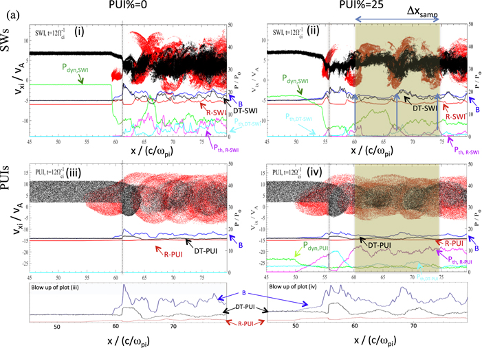
  ) is calculated separately for each ion population (PUIs and SWIs) and for R and DT ions within each ion species. Results are reported in Figure 6(a) for the cases PUI% = 0 (left panels) and 25 (right panels), and the density profiles of R (red curve) and DT (black curve) ion subpopulations are indicated as references. As expected for PUI% = 0, the upstream dynamic pressure (green curve) starts to drop to low values at the upstream edge of the SWI foot (at x/(c/ωpi) = 59.5 in plot (i)), and persists downstream, where it becomes comparable to the thermal pressure. This thermal pressure is carried mostly by the reflected component rather than the DT component in the 63 < x/(c/ωpi) < 70 range. Farther downstream (x/(c/ωpi) > 70), this energy is transferred to both R–SWIs and DT–SWIs in a comparative percentage through the thermalization of reflected ions, which progressively loose their coherent gyromotion when penetrating farther downstream. The distance plays the role of a filter in the energy distribution between PUIs and SWIs as long as the gyration of SWIs and PUIs maintain a certain coherency; over larger distances, a progressive diffusion takes place as their coherent gyromotion is lost.
Download figure:
Standard image High-resolution image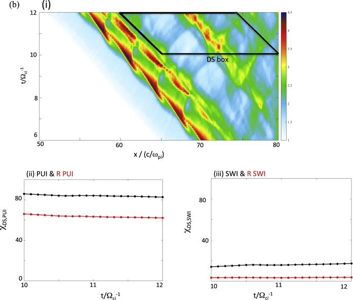
Figure 6. Panel (a) shows results obtained at the same fixed time t = 12  for different percentages of PUI% = 0 (run 1), and 25 (run 3), for SWIs (plots (i) and (ii)) and PUIs (plots (iii) and (iv)). Each panel includes a phase space plot (vxi–x) separately for the reflected (R) and directly transmitted (DT) ions shown by red and black dots, respectively; the profiles of the main magnetic field By (blue curve), of the density of R ions (red curve), and DT ions (black curve) are shown for each population. Profiles of the total ion dynamic pressure Pdyn = Ni
  (green curve), where Vxi, Vyi and Vzi are the ion bulk velocity components, and of the thermal pressure Pth = Ni
  calculated separately for R ions (magenta curve) and DT ions (cyan curve), are also shown. The vertical dashed lines indicate the ramp location where the amplitude of the field Elx is maximum. The yellow rectangle superposed in plots (ii) and (iv) illustrates the large sampling area (spatial width Δxramp = 60–74.8 c/ωpi at time t = 12
  ) used for the spatially averaged values of the pressure ratio shown in Figure 6(b) (see text). The bottom panels show a blow-up (extended y-scale) of the magnetic field (blue) and the density of DT–PUI (black) and of R–PUI (red) ions of panels (iii) and (iv), respectively. Panel (b) shows a time stackplot of the magnetic field By (plot (i)) within the time interval Δt = 6–12
  (for the case PUI% = 25 (run 3)); the superimposed trapeze represents the area covered by the large sampling box moving at velocity identical to the shock front velocity within the selected time interval Δt = 10–12
  (i.e., slightly more than one self-reformation cycle since Tref = 1.4
  (Table 2)); the width of the sampling box is fixed in time and its location, which is initially defined at Δxramp = 65–79.8 c/ωpi for t = 10
  , moves at Δxramp = 60–74.8 c/ωpi for t = 12
  (time of Figure 6(a)). The x profiles of the thermal pressure Pth,PUI, the total pressure Pth,tot = Pth,PUI + Pth,SWI, and their ratio χDS,PUI = Pth,PUI/Pth,tot have been calculated and spatially averaged within this spatial Δxramp. Results of
  (black curve) and of
  (red curve, where "DS" means "downstream") calculated at different times within two ion gyroperiods, are reported in plot (ii); similar ratios defined for SWIs are reported in plot (iii).
Download figure:
Standard image High-resolution imageHowever, the situation strongly differs for the case PUI% = 25 as follows: (i) the upstream dynamic pressure (green curve) drops to low values but is no longer transferred to the SWI population (regardless of which R–SWIs and DT–SWIs are concerned), since the thermal pressure becomes negligible for R–SWIs in the downstream region (magenta curve in plot (ii) of Figure 6(a)); (ii) most of the upstream SWI dynamic pressure is transferred downstream to PUIs, but this energy partition varies with distance (plot (iv) of Figure 6(a)). More precisely, the thermal pressure of DT–PUIs is dominant in the region (56 < x/(c/ωpi) < 58.5), where DT–PUIs suffer their first gyration immediately behind the ramp, but the situation reverses farther downstream (x/(c/ωpi) > 58.5), where the thermal pressure of R–PUIs largely and always dominates that of the DT–PUIs.
In order to estimate the impact on the downstream energy partition for PUI% = 25 more quantitatively, we have considered a downstream spatial range Δxsamp = 14.8 c/ωpi that is large enough to cover at least a few gyromotions of PUIs and many gyromotions of SWIs, as shown in Figure 6(a) (plots ii and iv), at a fixed time of the simulation; the subscript  means
means  . Within this range Δxsamp, we have calculated the space-averaged values of the thermal pressure Pth,PUI for the PUI population, the total ion thermal pressure Pth,DS (= Pth,PUI + Pth,SWI), and the resulting ratio χDS,PUI = Pth,PUI/Pth,DS; "DS" means "downstream." The same averaging calculation has been repeated at different times within a time interval covering two upstream inverse ion gyrofrequencies (i.e., slightly more than one self-reformation period tref = 1.4
  ), as the sampling box moves with a velocity equal to the shock front velocity vshock = −2.26 VA in the simulation frame (i.e., in the DS rest frame). This motion is illustrated by a parallepiped aligned along the shock front location and superimposed on the time stackplot of the main magnetic field (plot (i) of Figure 6(b)). Results of χDS,PUI versus time are reported in plot (ii) of Figure 6(b), which shows the following results: (i) the thermal pressure ratio χDS,PUI is around 84% (varies from 86% to 82.5%), which confirms that a large part of the downstream thermal energies are carried by PUIs; only a small part is carried by SWIs at a ratio of 16% (this varies from 14% to 17.5%); (ii) the ratio value χDS,PUI is almost independent of the time and comparable to the value (85%) obtained in Figure 7 of Wu et al. (2009) in a similar situation, where PUI% = 25. We note that
  (for R–PUIs only) is around 64% (varies from 66% to 62.5%), which confirms that most energy is carried by R–PUIs (panel ii). In contrast, the corresponding results shown for SWIs (panel (iii) of Figure 6(b)) show that χDS,SWI is around 14%, but the ratio
  (for R–SWIs only) stays around 4%, which means that the SWI energy is mainly carried by the DT–SWIs and not by the R–SWIs.
However, the almost constant value of χDS,PUI versus time needs to be improved by a more careful analysis. As mentioned in Section 1, the hybrid simulations of Wu et al. (2009) are based on the use of a space grid Δx = 1 c/ωpi, which eliminates any possible self-reformation of the shock front since the spatial resolution is not high enough, as reported by Hellinger et al. (2002). The situation strongly differs in the present case, where the self-reformation is obvious and still persists even in the presence of a noticeable percentage of PUIs (25%), as shown in Paper 1 and illustrated in our Figure 2. In order to clarify the situation, we recall that all ions on the downstream side (after being either once-reflected or DT) must have experienced the nonstationarity effects at the shock front and thus keep a "memory" of their passed trajectory. Then, smoothing any quantity over a large spatial range in the downstream region as done in Figure 6(b) is equivalent to "deleting" this memory effect, i.e to smoothing out the impact of the front nonstationarity. Then, two improvements have been brought: we have considered a much smaller spatial size of the sampling box (in order to keep a temporal/local signature of the energy partition), and this box is again moving at the main shock front velocity ("main" velocity means a velocity that is averaged over a self-reformation cycle and differs from the "instantaneous" shock front velocity, as detailed in Section 3 of Paper 1). The local thermal pressure has been calculated at different times within this local sampling box separately for SWIs and PUIs. The results are reported in Figure 7 for four different sampling boxes initially located at Δxsamp = 61–62, 63–64, 68–69, and 76–77 c/ωpi. The main features appear as follows: (i) the impact of the front nonstationarity is more clearly shown by the time fluctuations of χDS,PUI,loc and χDS,SWI,loc that are measured separately for PUIs and SWIs at short distance from the front (where the subscript "loc" means "local"); (ii) not too far from the shock front, these downstream quantities fluctuate around time-averaged values 18%–15% and 82%–85% for SWIs and PUIs, respectively; these mean values do not vary drastically for a greater distance downstream (17% and 83%); and (iii) the amplitude of these fluctuations tends to be smother when moving far downstream (Figure 7(e)). In short, these values are around constant values of 16% and 84%, respectively, as obtained within the large box of Figure 6(b). These "local" values are time-averaged over two upstream inverse ion gyrofrequencies (i.e., slightly more than one self-reformation cycle). We note that the time fluctuations of χDS,loc provide an additional signature of the impact of the front nonstationarity and can be used as helpful tools for theoretical models of the TS.
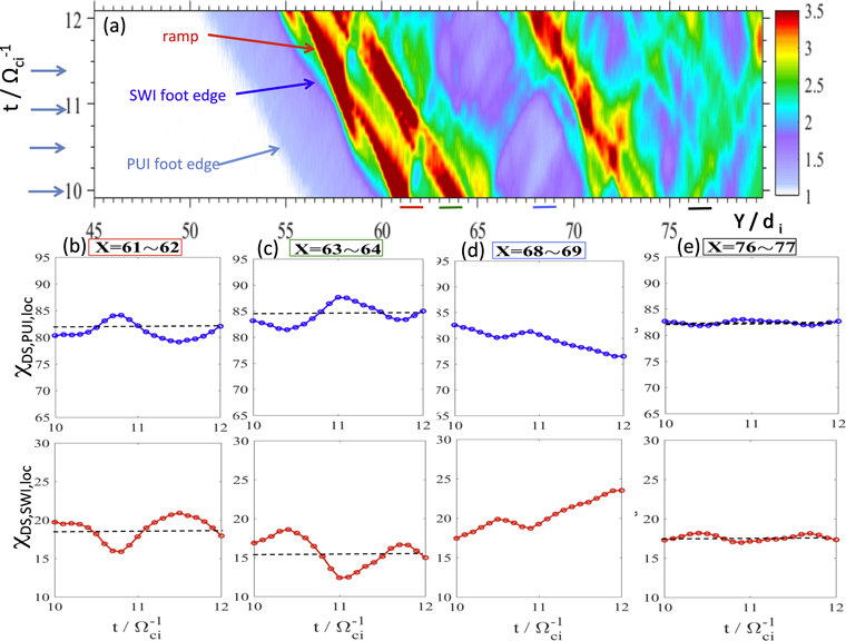
Figure 7. Time stackplot of the magnetic field strength By around the shock front for PUI% = 25 (run 3) shown in plot (a) within the selected time interval Δt = 10–12  . Different narrow sampling boxes (same width Δx = 1 c/ωpi) are indicated at different locations illustrated by colored bars (below plot (a)) within the downstream region (Δxsamp = 61–62 c/ωpi (red), 63–64 c/ωpi (green), 68–69 c/ωpi (blue), and 76–77 c/ωpi (black)) at the selected initial time t = 10
  ; these sampling boxes move at a velocity identical to the shock front velocity. The time history of the ratio χDS,SWI,loc = Pth,SWI/Pth,tot and χDS,PUI,loc = Pth,PUI/Pth,tot as defined for SWIs (blue curves) and the PUIs (red curves), respectively, measured within each sampling box is shown in plots (b–e); their time-averaged values are indicated by horizontal dashed lines.
Download figure:
Standard image High-resolution imageThe respective contributions of the dynamic and thermal pressures of the different ion populations (SWIs, PUIs, R, and DT) and of the magnetic field pressure are summarized in Figure 8 as a pie chart of the percentages in the upstream and downstream regions in order to provide a synoptic view of the pressure partitions. The case PUIs% = 10 was added for completeness. Figure 8 clearly shows how much upstream dynamic pressure (i) remains as dynamic pressure in downstream region, and (ii) is converted into thermal pressure and to electromagnetic pressure. More precisely, downstream thermal pressure is strongly carried by reflected PUIs; its contribution increases with PUIs% and becomes dominant for PUIs% = 25. Moreover, from upstream to downstream, the dynamic pressure Pd contribution of both PUIs and SWIs strongly decreases (as expected), while the magnetic pressure contribution PB strongly increases whatever the PUI% is. In addition, as PUIs% increases, (i) the downstream contribution of Pd,SWI decreases, while that of Pd,PUI increases (plots (e) and (f)), and (ii) the contribution of the downstream magnetic pressure PB decreases. In short, a higher PUI% is favorable for converting upstream dynamic pressure into more PUI thermal pressure, and into less SWI thermal pressure and electromagnetic pressure.
4.3. Impact of the Self-reformation on the Downstream Ion Distribution
The numerical results presented in the previous sections allow us to quantify in the total energy partition, the separate contribution not only of each ion population (SWIs and PUIs) and also of the respective subpopulation of ions that suffer different interactions with the shock front (namely the R and DT population separately for the SWI and PUI populations). Following the results of Section 4.2, a further investigation consists of analyzing now the impact of the front nonstationary on each ion subpopulation in the downstream region. Two main questions are addressed here: (i) how each subpopulation contributes to the total local ion distribution measured downstream and how it can be compared with previous models, and (ii) how this total distribution is affected by the nonstationary effects. Some results have been analyzed previously in a 1D PIC simulation (Yang et al. 2013, 2014; Lembege et al. 2014); later, 2D PIC simulations have been performed in plasma conditions identical to those used in 1D PIC, but without analyzing the impact of the nonstationarity along the shock normal versus along the shock front (Yang et al. 2015). We examine our present results with a deeper investigation and include nonstationarity effects along the shock normal only.
Furthermore, we recall that Zank et al. (2010) have previously postulated that the microphysics of the TS may play a key role in determining the form of the total downstream or heliosheath proton distribution, and have proposed a model of the local downstream/heliosheath ion distribution function as a superposition of three population components: (i) the transmitted relatively cool thermal SWIs, (ii) the transmitted PUIs, and (iii) the downstream hot PUIs that have been reflected at the TS. The model is reported in Figure 9(a), where the black curve describes the envelope of the total ion distribution, and where the heliosheath constructed proton distribution assumes that the transmitted PUIs possess a filled-shell distribution. Then, the envelope of the total distribution model is characterized by three different energy components that are illustrated by double arrows.

Figure 8. Pie chart of the dynamic and thermal pressures between the different ion populations and the magnetic pressure PB. The top and bottom panels represent results obtained in the upstream (US) and downstream (DS) regions, respectively. The left, middle, and right panels show the results of the cases PUI% = 0, 10, and 25. The colors are similar to those used in Figure 6(a), i.e., green (ion dynamic pressure), cyan (thermal pressure for directly transmitted ions), magenta (thermal pressure for reflected ions), and dark (magnetic pressure); "Pd" and "Pth" mean "dynamic" and "thermal pressure," respectively. Subscripts "SWI," "PUI," "R," and "DT" mean "solar wind ions," "pickup ions," "reflected," and "directly transmitted" ions, respectively. All measurements have been made at time t = 12  (same as Figure 6(a)). For the upstream region, measurements are made within the sampling ranges Δx = 42–59 c/ωpi , 42–52 c/ωpi, and 39–49 c/ωpi for PUI% = 0, 10, and 25, respectively, so that measurements are obtained from the leading edge of the large PUI foot to far upstream (no pollution by any gyrating SWI or PUI). For the downstream region, measurements are made from the shock front to far downstream, within the ranges Δx = 67–77 c/ωpi, 64–79 c/ωpi, and 60–75 c/ωpi for PUI% = 0, 10, and 25, respectively.
Download figure:
Standard image High-resolution imageIn order to validate the model, a comparison is performed with a local ion distribution function measured downstream and issued from our self-consistent PIC simulation. Figure 9(b) shows not only the total downstream distribution measured at a given time t = 10  of the simulation within the sampling box Δxsamp = 76–78 c/ωpi, but also the different ion populations contributing to the total ion envelope: full and dashed red curves show R–SWIs and DT–SWIs, respectively, and full and dashed blue curves show the R–PUIs and DT–PUIs, respectively. The main results clearly show that the total ion population obtained self-consistently from our PIC simulations (black curve) is very near the model proposed by Zank et al. (2010). A deeper analysis of our results emphasizes the following points: (i) the low-energy component (called the cool component in Zank et al. 2010) corresponds well with the DT–SWIs (dashed red curve); in contrast, the high-energy component corresponds to the energetic R–PUI population (full blue curve). The intermediate-energy component is carried by both the R–SWIs (full red curve), which has been neglected in Zank et al. (2010), and by the DT–PUI component (dashed blue curve). Except for the evidence that R–SWIs cannot be neglected in a self-consistent approach, our results are in reasonable agreement with Zank et al. (2010) and allow us to validate their model. In addition, our results provide more quantitative information on the relative contribution of each population to the total distribution envelop.
The last following questions are whether this agreement persists when the nonstationary effects at the shock front are included in a self-consistent approach (i.e. self-reformation)? How is the contribution of the four subpopulations to the total distribution affected by the self-reformation? To answer these questions, we have performed similar measurements of the different ion distributions within the same moving sampling box (Δxsamp = 2 c/ωpi; for reference, the box is located at Δxsamp = 76–78 c/ωpi for t = 10  ) at different times within a given self-reformation cycle, namely at times t = 10, 10.5, 10.9, and 11.3
  , as marked by the four arrows in Figure 7(a). The corresponding results are shown in Figure 10, where the three different energy components within the total population are highlighted by three colored areas in order to emphasize their identification. The main results may be summarized as follows : (i) the three energy components persist quite well regardless of the time, (ii) the low-energy component (blue area) stays mainly controlled by the DT–SWI population and is almost unchanged for the "coolest" part regardless of the time, but slightly interacts with the R–SWIs (full red curve) in its wings; (iii) the high-energy component (red area) stays mainly controlled by the R–PUIs that dominate, and is almost unchanged regardless of the time, and (iv) in the intermediate-energy component (green area), however, the DT–PUI population (dashed blue curve) strongly contributes together with R–SWIs; both subpopulations "interact" versus time in their respective contributions. This "interaction" can be illustrated, where DT–PUIs (dashed blue line) contribute mainly to the left-hand wing of this energy component at all selected times, and less strongly to the right-hand wing; in contrast, R–SWIs contribute to the right-hand wing in a comparable way with DT–PUIs at t = 10 and 10.9
  . One noticeable point is the strong variation in the R–SWI population (full red curve) versus time; this feature is expected since the SWIs drive the self-reformation via the R–SWIs that are directly impacted. In summary, the nonstationarity of the shock does not have a drastic impact on the "global" shape of the total ion population. More precisely, the low- and high-energy components are slightly affected; however, the intermediate-energy component varies more in the sense that the internal energy is redistributed in time between the different ion subpopulations supporting this energy component.
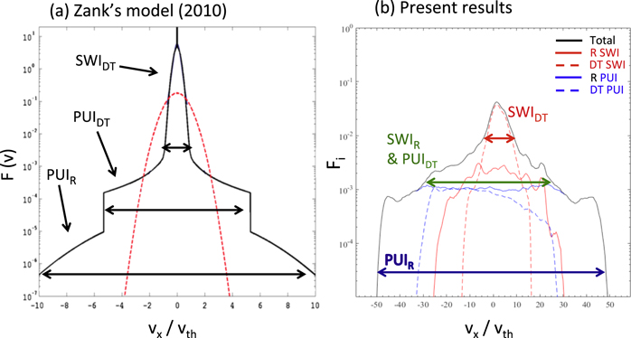
Figure 9. Panel (a) shows the model of the total local downstream distribution function proposed by Zank et al. (2010), which is a superposition of three population components: (i) transmitted relatively cool thermal SWIs (so-called SWIDT), (ii) the transmitted PUIs (so-called PUIDT), and (iii) downstream reflected PUIs (so-called PUIR), which have been reflected at the TS, as indicated by arrows; the resulting heliosheath constructed proton distribution assumes that the transmitted PUIs possess a filled-shell distribution. The particle velocity vx is normalized to the Maxwellian thermal velocity vth = 2 kT/mi, where k is the Boltzmann constant and T is the total ion downstream temperature; the red curve illustrates a Maxwellian distribution (used as reference) with the downstream ion density and temperature. Panel (b) shows the corresponding total local distribution function measured in our PIC simulation, within the sampling box Δxsamp = 76–78 c/ωpi at time t = 10  for the case PUI% = 25 (run 3). The distribution includes the contribution of the R–SWIs (full red curve), DT–SWIs (dashed red curve), R–PUIs (full blue curve), DT–PUIs (dashed blue curve), and the envelope of the total distribution (black curve).
Download figure:
Standard image High-resolution imageAt least, we note that two different downstream ion distribution models have been proposed by Zank et al. (2010), in which the transmitted PUIs evolve into a Maxwellian distribution or possess a filled-shell distribution, respectively (as illustrated in Figure 9(a)). Our simulation results retrieve self-consistently a filled-shell distribution, which is a quite appropriate model, and the agreement between our simulation results and this model persists in time (except for the change in the relative contributions of the different ion subpopulations within the intermediate-energy component, and partially within the low-energy component). In order to support this statement, we have measured the 3D ion velocity space (vx, vy, vz) in the same sampling box and at the same times as in Figure 10. The results shown in Figure 11 confirm that the total downstream PUI distribution (including both R ions (red dots) and DT ions (black ions)) can be well described by a filled-in shell since the filling of the initial upstream zero-thickness shell is generated by the turbulence developed in the downstream region (Figures 11(b)–(e)). This filling is clearly illustrated by comparison with the initial zero-thickness shell shown in Figure 11 as a reference. We note that the flat-top shape of the PUI distribution F(vx) measured in Figure 4(b) for both R–PUIs and DT–PUIs is only a 2D reduced representation of this 3D filled-in shell PUI distribution after cutting along the vx component at the location where vy = vz = 0. Figure 4(b) also confirms that the initial shell is well filled-in in the downstream region, and is partially filled-in over the upstream region Δx = −10 c/ωpi (from the ramp), which includes all freshly reflected R–PUIs.
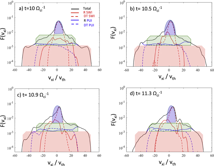
Figure 10. Results issued from our PIC simulations; plots (a–d) are similar to Figure 9(b) and measured at different times t = 10, 10.5, 10.9, and 11.3  , chosen within one self-reformation cycle of the shock front (indicated by thick arrows on the left-hand side of Figure 7(a)) within the moving sampling box located at Δxramp = 76–78 c/ωpi at initial time t = 10
  . The three energy components discussed in the text are highlighted by red, green, and blue areas.
Download figure:
Standard image High-resolution imageWe note that in the model of Zank et al. (2010), the particle velocity vx is normalized to the Maxwellian thermal velocity vth = 2 kT/mi, where k is the Boltzmann constant and T is the total ion downstream temperature. A similar normalization has been performed and applied to the measurements of Figure 10 (not shown here), which confirms that all the main previous results mentioned above are unchanged.
The results of Section 4.2 have indicated that the local time-averaged values of the ratios χDS,SWI,loc and χDS,PUI,loc vary versus the downstream location of the sampling box (Figure 7). Then, a last point consists of analyzing how the local ion distribution varies versus the downstream distance and for different widths of the sampling box at a fixed time. The results illustrated in Figure 12 emphasize the following points: (i) the three energy components are still well identified; (ii) the features of the low-energy component are unchanged (blue area); (iii) in contrast, the distance from the front has some impacts on the high-energy component (red area), which may be carried either by both DT–PUIs and R–PUIs (at short distance from the front, as illustrated by the contributions of the left-hand shoulder of DT–PUIs, and the right-hand shoulder of R–PUIs in plot (b)), either by R–PUIs alone farther downstream (as in plots c–d) or within a very large downstream sampling box (as in plot e); (iv) again, the energy distribution between the different ion subpopulations strongly varies within the intermediate-energy component (green area); and (v) as the distance increases downstream, the contribution of R–SWIs (full red curve) suffers the largest variation.

Figure 11. Results issued from our PIC simulations. Three-dimensional plots of the PUIs velocity space measured upstream at time t = 0 (a) and within the same (moving) downstream sampling box as for the times of Figure 10 (b)–(e). R–PUIs and DT–PUIs are identified by red and black dots.
Download figure:
Standard image High-resolution image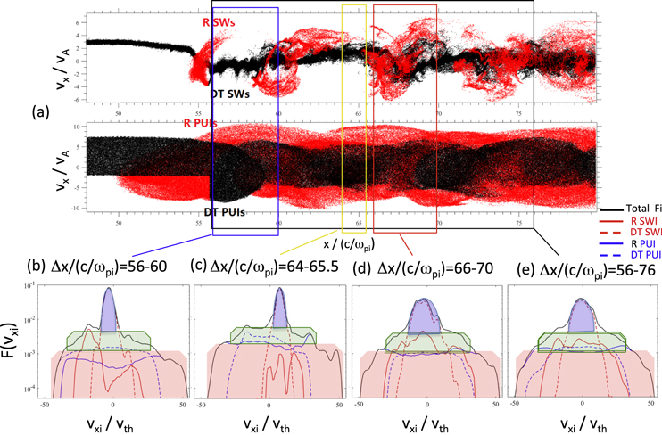
Figure 12. Measurements similar to those of Figure 10 obtained within sampling boxes of different sizes and at different locations, but at the same fixed time t = 12  ; these are defined by Δxramp = 56–60 (b), 64–65.5 (c), 66–70 (d), and 56–76 c/ωpi (e); the locations of the boxes are superimposed on the ion phase space shown in plot (a).
Download figure:
Standard image High-resolution image5. Discussion and Conclusions
In this paper, we use the 1D electromagnetic PIC code that self-consistently includes PUIs, SWIs, and electrons in order to analyze the impact of both shock front nonstationarity and the presence of PUIs on the energy exchanges between the different ion populations through a strictly perpendicular shock. More precisely, the mutual impacts of the front nonstationarity on the distribution functions of each population at/around the shock front and far downstream and on the energy partition between the different ion components have been investigated. In particular, a deep analysis has been performed by separating the SWI and PUI populations into two parts: R and DT. Our main results may be summarized as follows:
- (a)The shock front nonstationarity still persists even in the presence of a noticeable percentage of PUIs (25%), as found in the experimental results of the Voyager-2 mission at the heliospheric TS. In return, this nonstationarity (here supported by the front self-reformation) has an important impact on both the SWI and PUI populations and on their respective energy partition.
- (b)As the PUI% increases, the time-averaged value of the ion reflection rate decreases noticeably for both PUIs and SWIs. The amplitude of the time fluctuations due to the front nonstationarity stays relatively moderate, and it is smoothed out with PUI% increase.
- (c)Our results provide quantitative information on the contributions of R and DT ions separately to local SWI and PUI distributions at different locations: at/around the shock front (i.e., near upstream and downstream of the ramp) and within the far downstream region. In the region near/around the shock front, (i) both R- and DT–SWIs gain high energy when moving from upstream to downstream, but the maximum energy range is much larger for the PUIs (than for SWIs) and is mainly carried by the R–PUIs; (ii) for all PUI% cases, the gain in energy downstream is higher for R ions than for DT ions for both SWIs and PUIs; (iii) the maximum downstream energy range for R–SWIs decreases as PUI% increases, while it stays almost independent for DT–SWIs regardless of the PUI%; (iv) the R–SWI distribution approaches a flat top, which suggests a strong contribution from the Elx field. However, the situation differs for the PUIs as follows: (i) the downstream R–PUI and DT–PUI distributions always have a flat-top shape; (ii) the most energetic PUIs correspond to the R–PUIs that reach the downstream region after suffering only one large gyromotion; and (iii) one striking feature is that the upstream R–PUI distribution (including all freshly reflected R–PUIs) is a superposition of a flat-top and a local beam centered around a drift value Vdx/VA = −3. This feature is currently under investigation and will be analyzed in a separate study.
- (d)A complementary analysis of the energy partition has been performed within very large downstream sampling regions (where the impact of the front nonstationarity tends to be smoothed out). Spatially and time-integrated results confirm that the major part of the incoming dynamic pressure is transferred downstream mainly as thermal pressure to PUIs (around 86%–82.5%) and not to SWIs (only 14%–17.5%). These values are in good agreement with previous works that were based on hybrid simulations. More precisely, the energy is mainly transferred to both R–PUIs and DT–PUIs in the downstream region immediately after the shock front, and only to R–PUIs further downstream.
- (e)However, our results show that the concerned sampling procedure (width and location of the sampling box) also has some impacts, as shown in the downstream measurements made within a small (instead of a very large) size of the sampling box moving with the same velocity as the shock front. First, the use of a small box clearly shows the time fluctuations in the energy transfer (illustrated by the quantity χDS,loc) that are due to the self-reformation of the front; this applies to both SWIs and PUIs. Second, the amplitude of these fluctuations is larger within a box that is located near the front, and tends to be smoothed out as the distance from the shock increases. Third, the
 time-averaged values of χDS,loc may vary when measured at different distances farther downstream, but do not change drastically (χDS,loc = 82%–85% for PUIs, and χDS,loc = 18%–15% for SWIs).
 - (f)Local downstream ion velocity distribution functions have been analyzed in detail in order to compare our results with previous works. We found that the total downstream ion distribution Ft function is a superposition of four subpopulations (R–SWIs, DT–SWIs, R–PUIs, and DT–PUIs), and allows us to identify three characteristic energy components: (i) a low-() energy component mainly carried by the DT–SWIs, (ii) a high-energy component mainly carried by the R–PUIs, and (iii) an intermediate-energy component mainly carried by a mixture of R–SWIs and DT–PUIs. The shape of the total distribution function is in reasonable agreement with an early model for heliosheath particles proposed by Zank et al. (2010), and allows us (i) to validate their model based on a filled-in shell used to describe downstream DT–PUIs (rather than a Maxwellian population) and (ii) to confirm that one missing subpopulation (R–SWIs) would need to be added in the model of Zank et al. (2010) for a full agreement.
- (g)Moreover, the situation becomes more complex as the nonstationary effects are now included. Indeed, the downstream function is shown to be affected by the turbulence created by both (i) the phase mixing of SWI and PUI populations and (ii) by the time shock front self-reformation. The contributions of each subpopulation evolve in time under the impact of the self-reformation process. More precisely, our statistics show that (i) the identification of three energy components persists well in time, (ii) R–PUIs always dominate the high-energy component in time; however, (iii) the intermediate-energy component is dominated by an between DT–PUIs and R–SWIs, and (iv) low-energy component is dominated by an interplay between DT-SWIs (main contribution) and R–SWIs. Then, the R–SWI population has a certain impact on both the low- and intermediate-energy component, which can be interpreted as a consequence of the fact that R–SWIs mainly drive the self-reformation itself (see paper 1). As a consequence, the missing subpopulation (R–SWIs) in the Zank et al. (2010) model cannot be neglected when nonstationary effects are included.
- (h)Our PIC simulation results may be compared with some statements of Kucharek et al. (2010) based on 2D hybrid simulations. These authors reported that in order to produce ENAs in an efficient way, one requires an ion source population that is streaming sunward and is ideally beam-like; a gyrating distribution represents such a population for the TS, which is quasi-perpendicular since its pitch angle distribution is centered around 90° and aligned to the shock normal, and an important part of the ions points sunward. The authors came to the conclusions that the reflected solar wind at the TS could be an appropriate candidate for a quite intense ENA source. Our results are partially in agreement with these results. More precisely, we find that R–SWIs form a clear beam with a negative bulk velocity Vxi = −1.3 VA (i.e., directed sunward, as shown in plot (iii) of Figure 4(a)) for PUI% = 25. Moreover, some differences are observed with respect to the results of Kucharek et al. (2010) as follows: (i) we observe this R–SWI beam not only for PUI% = 25, but also for a moderate percentage PUI% = 10 (plot (ii) in Figure 4(a)), (ii) for high percentage PUI% = 25, the SWIs look more heated and the associated beam bulk velocity Vxi looks lower than for lower PUI% = 10, in apparent disagreement with Kucharek et al. (2010). We have to keep in mind, however, that the results presented in Figure 4 have been obtained at the same fixed time for all cases PUI% = 0, 10, and 25, and the microstructures of the shock front and the energy partition vary in time because of the shock front nonstationarity (self-reformation); then, the relative bulk motion and heating of the beam will vary as well. The self-reformation along the shock normal has not been included in the 2D hybrid of Kucharek et al. (2010) since the spatial resolution they used was too low (Δx = 0.5 c/ωpi, while self-reformation requests a grid Δx lower than 0.5 c/ωpi, as shown by Hellinger et al. 2002). This self-reformation may also impact the clarity of the beam signature. (iii) At least, our results also show a (partial) sunward beam that is superimposed on the flat-top part of the local R–PUI distribution (plots (ii) and (iii) of Figure 4(b)); the associated bulk velocity stays almost unchanged around Vxi = 2.5–3 VA for PUI% = 10 and 25; this beam was not mentioned in Kucharek et al. (2010). Then, our results show that sunward beams are observed upstream in both R–SWI and R–PUI distributions and represent viable candidates for a production source of ENAs (the R–SWI beam has a much stronger signature), but their relative beam features may vary in time, which also affects the local efficiency of ENAs production, a fact which has not been taken into account in previous works. Downstream of the shock, mainly flat-top distributions have been identified instead of beams in our work. The reason is that relatively large sampling boxes have been used (Δxsamp = 10 c/ωpi) in the close vicinity of the shock front, while boxes of smaller size are necessary to show beam patterns as a part of the gyrating SWIs and/or PUIs. Indeed, in the downstream vicinity of the shock front, sunward beam and downstreaming pointing beam are clearly visible in the R–SWI distributions (red full line in plot (b) of Figure 12) when small-size sampling boxes are used; however, no clear beam appears in the R–PUI distribution, which only shows some shoulder (blue full line). Farther downstream, only a downstreaming pointing beam persists in the R–SWI population (plot (c) of Figure 12). Far downstream, any beam pattern disappears at any time of the self-reformation in both SWI and PUI subpopulations, even when the measurement is performed within a very narrow sampling box (Figure 10 and plot (d) of Figure 12), which means that downstream populations cannot be viable sources of ENAs production when they are too far removed from the front. In summary, the attention must be focused only on the near vicinity of the shock front where upstream/downstream R–SWIs are shown to be a strong viable candidate, and upstream R–PUIs can only be another secondary candidate.


The results of Paper 1 have provided helpful information to modelers for describing the microstructures of the TS. Our results obtained within a self-consistent approach and taking into account the time/spatial scales of all populations provide complementary and detailed helpful information for modeling the time variation of the energy partition, the distribution functions measured at/around the shock front and far downstream, and the time-varying contributions of the different subpopulations. More precisely, these results suggest some theoretical refinements to model more precisely the different subpopulations that contribute to the total downstream distribution and the impact of the front nonstationarity.
The Centre National d'Etudes Spatiales (CNES) in France is acknowledged for its support. A large part of the numerical simulations has been done on the IDRIS computer center located at Orsay (near Paris) which is thanked for its support. The research is also partially supported by NFSC under Grant No. 41574140 and 41374173, the Open Research Program Key laboratory of Geospace Environment CAS, Youth Innovation Promotion Association Funding No. 2017188, Strategic Priority Program on Space Science No. XDA15011300, and Beijing Excellent Talent Training Project Funding No. 2017000097607G049, and the Specialized Research Fund for State Key Laboratories of China. The authors wish to thank G. Zank for stimulating discussions. The referee is thanked for helpful remarks on the manuscript.