


Abstract
Low-resolution Spitzer-IRS spectral map data of a reflection nebula (NGC 7023), H ii region (M17), and planetary nebula (NGC 40), totaling 1417 spectra, are analyzed using the data and tools available through the NASA Ames PAH IR Spectroscopic Database. The polycyclic aromatic hydrocarbon (PAH) emission is broken down into PAH charge and size subclass contributions using a database-fitting approach. The resulting charge breakdown results are combined with those derived using the traditional PAH band strength ratio approach, which interprets particular PAH band strength ratios as proxies for PAH charge. Here the 6.2/11.2 μm PAH band strength ratio is successfully calibrated against its database equivalent: the  ratio. In turn, this ratio is converted into the PAH ionization parameter, which relates it to the strength of the radiation field, gas temperature, and electron density. Population diagrams are used to derive the
  density and temperature. The bifurcated plot of the 8.6 versus 11.2 μm PAH band strength for the northwest photo dissociation region in NGC 7023 is shown to be a robust diagnostic template for the
  ratio in all three objects. Template spectra for the PAH charge and size subclasses are determined for each object and shown to favorably compare. Using the determined template spectra from NGC 7023 to fit the emission in all three objects yields, upon inspection of the Structure SIMilarity maps, satisfactory results. The choice of extinction curve proves to be critical. Concluding, the distinctly different astronomical environments of a reflection nebula, H ii region, and planetary nebula are reflected in their PAH emission spectra.
Export citation and abstract BibTeX RIS
1. Introduction
The mid-infrared (IR) spectrum of many astronomical objects in the Milky Way and many other galaxies, including H ii regions, reflection nebulae (RNe), the interstellar medium (ISM), regions of massive star formation, etc., is dominated by emission from large polycyclic aromatic hydrocarbon (PAH) molecules, clusters, and aromatic rich, very small (nano-)carbon grains (e.g., Werner et al. 2004; Berné et al. 2007; Draine & Li 2007; Smith et al. 2007b; Tielens 2008; Boersma et al. 2012; Mori et al. 2012; Peeters et al. 2012; Riechers et al. 2014; Stock et al. 2014; Hemachandra et al. 2015; Shannon et al. 2015; Stock et al. 2016 and references therein). Since emission spectra from these species depend on the local radiation field, temperature, and state of the PAH population in terms of size, charge, structure, and composition, they contain a wealth of information about the local physical environment and the evolutionary history of cosmic carbon.
To extract this information from the astronomical PAH spectrum, several tools have been developed (e.g., PAHFIT, Smith et al. 2007b; PAHTAT, Pilleri et al. 2012). However, these tools rely to a large extent on top-down, empirical approaches that require an ad hoc generic astronomical PAH spectrum that carries with it assumptions regarding the PAH properties, such as charge, size, structure, composition, and so on. This paper, based on a self-consistent, bottom-up approach, avoids any assumptions about astronomical PAH spectra by combining a large library of authentic PAH spectra comprised of PAHs of different charge states, sizes, structures, and compositions with a set of straightforward tools that can fit astronomical spectra and break the PAH emission down into contributing PAH subclasses, i.e., charge, size, composition, and structure. In doing so, traditional qualitative PAH band strength ratio proxies can be put on a quantitative footing.
Here the work reported in Boersma et al. (2016; hereafter BBA16) on the spatial behavior of the PAH emission bands and PAH population changes within and between RNe is extended to include a planetary nebula (PN) and H ii region. The approach builds on that described in detail in Boersma et al. (2013; hereafter BBA13), Boersma et al. (2014a; hereafter BBA14), and Boersma et al. (2015; hereafter BBA15). NASA's Spitzer Space Telescope (Werner et al. 2004) obtained spectral maps of these objects utilizing its IR spectrograph (IRS; Houck et al. 2004). The spectra comprising these maps are analyzed using the data and tools made available through the NASA Ames PAH IR Spectroscopic Database (PAHdb1 ; Bauschlicher et al. 2010; Boersma et al. 2014a; A. L. Mattioda et al. 2018, in preparation).
Focusing on PAH charge, there are three main goals to this work: (1) determining if the PAH database-fitting approach provides consistent results within and between a RN, H ii region, and PN; (2) relating the derived ionized fraction to the PAH ionization parameter, which allows one to determine the radiation field, electron density, and temperature of the gas in each object; and (3) evaluating the validity of using PAH spectroscopic templates, also known as PAH principal-component spectra, within and between RNe, H ii regions, and PNe. Principal-component spectra are now commonly used for the analysis and interpretation of astronomical PAH spectra (e.g., Rapacioli et al. 2005; Berné et al. 2007; Rosenberg et al. 2011; Pilleri et al. 2012; BBA13; BBA16).
The outline of this paper is as follows. Section 2 summarizes the observations and the reduction of the data. In Section 3, a stepwise description of the analysis is given. The results are presented in Section 4, followed by a discussion in Section 5. This work is finalized in Section 6, where a summary with conclusions is given.
2. Observations and Data Reduction
The three targets studied here have been observed with the IRS (Houck et al. 2004) onboard the Spitzer Space Telescope (Werner et al. 2004). Table 1 summarizes the observations. Although high-resolution, short–high (SH) spectroscopic data from 10 to 20 μm are available for these targets, the 5.2–14.5 μm low-resolution, short–low (SL) spectroscopic data are analyzed here, since they cover the bandwidth that includes the major PAH features while avoiding the uncertainties introduced by combining spectra taken with different instruments and resolution. The following subsection describes the targets, followed by a detailed description of the data reduction process.
Table 1. Summary of the Spitzer-IRS Observations and Astronomical Parameters
| Target | R.A.a | Decl.a | Sizeb | Observer(s) | Program ID(s) | dc | Irradiating Star | Stellar Typed |
 e
e
|
|---|---|---|---|---|---|---|---|---|---|
| (h m s) |
 arcmin arcsec) arcmin arcsec) |
(pixels) | (pc) | (K) | |||||
| NGC 7023 | 21 01 32.1 | +68 10 14 | 195 | Fazio | 28 | 430 | HD 200775 | B2Ve | 20,600 |
| M17 | 18 20 20.8 | −16 12 58 | 1045 | Wolfire | 30295 | 1814 | CEN1 | O4+O4 | 41200 |
| NGC 40 | 00 13 01.2 | +72 31 23 | 177 | Weedman | 50834 | 1249 | WD | WC8 | 90,000 |
Notes.
aCoordinates are in the J2000 system and for the center of each of the constructed, combined spectral maps. bSize is the total number of nonmasked pixels for each target. cIndividual distance references for each target are given in Section 2.1. dStellar types are taken from the SIMBAD (Wenger et al. 2000). Individual stellar type references for each target are given in Section 2.1. eThe effective stellar temperature, where appropriate, has been inferred from the stellar type using Table 5 from Pecaut & Mamajek (2013).Download table as: ASCIITypeset image
2.1. Targets
NGC 7023. NGC 7023 is the RN in Cepheus irradiated by the B2Ve (Rogers et al. 1995), massive spectroscopic binary (Millan-Gabet et al. 2001), Herbig Be star HD 200775. It is located some 430 pc from Earth (van den Ancker et al. 1997). The left panel in Figure 1 presents the morphology of NGC 7023's northwest photodissociation region (PDR) for which Spitzer-IRS spectral map data are available. This PDR was previously studied in BBA13, BBA14, BBA15, and BBA16 employing the database-fitting technique used here. Other recent work studying the PAH emission from this source include Berné et al. (2007), Rosenberg et al. (2011), Pilleri et al. (2012), Stock et al. (2016), and Croiset et al. (2016).
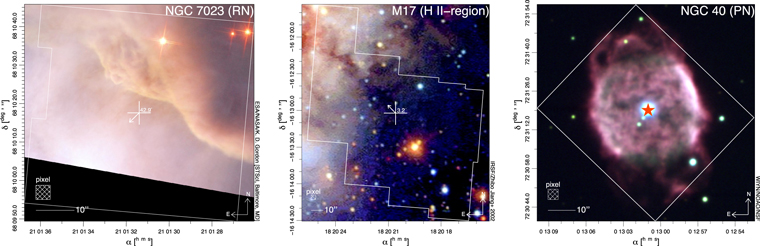
Figure 1. Left: RN NGC 7023 Spitzer-IRS field (white border) superimposed on a composite Hubble Space Telescope ACS image of part of the northwest PDR in NGC 7023. Combined Hα and IR I-band data are shown in red, optical V-band data in green, and optical B-band data in blue. Image credits: ESA/NASA/K. D. Gordon (STScI, Baltimore, Maryland). The white arrow points in the direction of HD 200775, located some 43'' from the center of the map, just outside the field of view. Middle: H ii region M17 Spitzer-IRS field (white border) superimposed on a IRSF/SIRIUS image of M17. The J-band data are shown in blue, H-band data in green, and Ks-band data in red. Image credits: Jiang et al. (2002). The white arrow indicates the direction of CEN1, located 3 2 from the center of the field. Right: PN NGC 40 Spitzer-IRS field (white border) superimposed on a WIYN image of NGC 40. The B-band data are shown in blue, V-band data in green, and R-band data in red. Image credits: NOAO/AURA/NSF. The orange star shows the position of the Wolf–Rayet star at the center of the nebula. The Spitzer-IRS pixel size utilized in this work is indicated by the labeled box in each image.
Download figure:
Standard image High-resolution imageM17. M17 is the massive young star-forming region located in Sagittarius, some 1800 pc from Earth (Kharchenko et al. 2005). It is one of the most massive nearby star formation regions in the Galaxy (Povich et al. 2009). The most luminous of the seven ionizing O stars in M17 is the binary system CEN1 (Chini et al. 1980). The middle panel of Figure 1 presents the morphology of M17 around the southwest photodissociation front—located in its southern bar—as seen by the SIRIUS (Nagashima et al. 1999) instrument at the IRSF 1.4 m telescope that covers the area for which Spitzer-IRS spectral map data are available. The data cover an enormous 1' × 1' (∼1 pc2) area and trace emission from just beyond the hard H ii region–PDR boundary, located about 10'' (∼0.09 pc) from the northeastern corner of the field, to well into the giant molecular cloud (38; ∼2 pc). The spectral map data overlap with ISO-SWS observations studied by Verstraete et al. (1996), albeit avoiding the H ii region directly where PAHs are unlikely to survive the harsh environment. The well-known PAH emission in M17 has most recently been studied by Povich et al. (2007), Doney et al. (2016), Stock et al. (2016), and Yamagishi et al. (2016).
NGC 40. NGC 40 is the PN located in Cepheus some 1250 pc from Earth (Stanghellini et al. 2008). NGC 40 is well studied and considered unusual when compared to the majority of Galactic PNe, notably because it shows spectral variability on a scale of hours (Balick et al. 1996; Grosdidier et al. 2001). Modeling the spectrum of the late-type WC8 Wolf–Rayet exciting central star suggests an effective temperature of up to 90,000 K (Bianchi & Grewing 1987; Leuenhagen et al. 1996; Marcolino et al. 2007). The right panel in Figure 1 presents the morphology of the region as seen by the WIYN/ESO 3.5 m telescope that covers the area for which Spitzer-IRS spectral map data are available.
2.2. Data Reduction
The Spitzer-IRS low-resolution observations for the three targets were downloaded from the Spitzer Heritage Archive (SHA). The spectra cover 5.2–14.5 μm at a resolution of  /Δλ ∼ 64–128. The spectral maps were assembled using CUbe Builder for IRS Spectra Maps (CUBISM; Smith et al. 2007a) in its default configuration with the most recent calibration files. CUBISM's automatic bad-pixel-generation parameters were set to
  and Minbad-fraction=0.5 and 0.75 for the global and recorded bad pixels, respectively. Spurious data at the ends of the SL slit were ignored by applying a wavsamp of 0.05–0.80. A rather large 0.2 cut at the high end was necessary to avoid striping artifacts that would appear for some of the lower signal-to-noise data, notably those with redundancies along the slit. No separate sky subtraction was performed due to the lack of such data. Since a local continuum is established and subtracted before isolating the PAH emission bands (see Section 3), and the actual sky is not expected to have much substructure; this does not pose a problem. The extracted SL orders SL1 and SL2 were written to file, after which remaining bad, NaN-valued pixels were interpolated in the spatial domain. With the help of the IDL Astronomy Library (Landsman 1993), the constructed spectral maps were resampled, combining 2 × 2 pixels, reaching an ultimate pixel size of 3
 6 × 36. Note that no spatial corrections were applied for the wavelength-dependent point-spread function (PSF). The SL1 and SL2 data were spatially aligned and combined into a single data cube, where the SL2 order was multiplicatively spliced to the SL1 order by conserving integrated flux in the spectral region of overlap. Following this, the spectra were σ-clipped, where the flux contained in each resolution element was evaluated with respect to the mean of its two preceding and two following spectral elements. If the flux in the resolution element under consideration was removed three or more standard deviations from the surrounding mean, it was replaced with the linear interpolant across the adjacent elements. Lastly, a mask was constructed recording pixels with no spectrum in the sparse maps and pixels with a spectrum of low-quality and/or "abnormal" structure, e.g., spectra showing a strong hot dust continuum component associated with embedded sources.
Errors were propagated by taking the squared uncertainty maps from CUBISM and performing the same reduction steps as on the spectral data while assuming additive uncertainties ( ). Uncertainties from splicing and σ-clipping are ignored but are not expected to exceed 10%.
2.3. Clustering
For each target, the spectra have been organized into bins using hierarchical clustering with a divisive scheme. A similarity matrix is constructed from the pairwise summed Euclidean distance norm of each two spectra, which were normalized to the total integrated intensity at each pixel.
As with k-means clustering, the established cluster bins divide the region into comparable morphological neighborhoods (zones) that can be used to help visualize spectroscopic and PAH population changes across them (see e.g., BBA14). In this study, two iterations, resulting in  cluster bins, with a minimum of 10 spectra for a cluster bin, proved sufficient to map the salient spectral changes across each target.
Figure 2 presents the average 5.2–14.5 μm Spitzer-IRS spectrum of each bin for each target, and Figure 3 overlays the location of the spectra associated with each bin, hereafter referred to as zones, onto the overview image of each target.
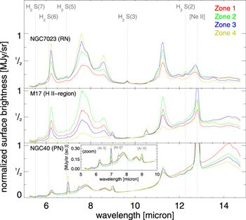
Figure 2. Four average 5.2–14.5 μm Spitzer-IRS spectra for each cluster bin/zone identified through hierarchical clustering, illustrating the range of spectral variation across each of the targets. See Section 2.3 for details. For display purposes, the spectra are shown first normalized to their intensity at 10 μm before being normalized to their peak intensity, while ignoring the contributions from any strong emission lines. Indicated are the  emission lines, together with the [Ne ii] atomic line near 12.8 μm. The inset of the bottom panel zooms in on the 5–10 μm region of NGC 40, indicating some additional atomic lines present in some of the spectra. The color of each spectrum indicates the associated zone in Figure 3.
Download figure:
Standard image High-resolution image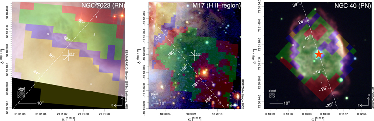
Figure 3. Same images as in Figure 1, now overlain with the four zones identified through hierarchical clustering and numbered 1–4. The average spectrum of each zone is shown in Figure 2, indicated by the associated zone color shown here. Also shown is a line connecting the star with a reference point within the field, such that it is perpendicular to the PDR. The distance from the irradiating source is indicated in arcseconds. The left, middle, and right panels show NGC 7023, M17, and NGC 40, respectively. See Section 2.3 for details.
Download figure:
Standard image High-resolution imageThe advantage of hierarchical over k-means clustering is that zone structures tend to better reflect discontinuities in the underlying morphology. This is because k-means clustering is based on average spectra, while hierarchical clustering, as used here, is based on spectral differences.
Keep in mind that the analysis and description that follow treat the data on a pixel-by-pixel basis and do not involve clustering techniques. However, the zones established through clustering are used to track comparable spectra—which are connected to morphologically similar regions—throughout the analysis and interpretation of the results.
3. Analysis
The data analysis consists of the following five steps.
- 1.Isolating the PAH emission spectrum. Emission that originates in PAHs is separated from emission due to non-PAH components, i.e., the underlying continuum and emission lines associated with molecular hydrogen and atomic species; see Section 3.1.
- 2.Fitting the PAH emission spectrum. The complete PAH emission spectrum (not individual bands) is fitted using the data and tools made available through PAHdb, which enables one to break the emitting PAH family down into contributing PAH subclasses, i.e., charge, size, composition, and structure; see Section 3.2.
- 3.Determining PAH band strengths. Individual PAH band strengths are determined using the traditional approach of isolating the PAH features from the continuum, their underlying plateaus, and removing where necessary molecular hydrogen and/or atomic emission lines. The individual PAH band strengths are then determined and combined into ratios commonly used as qualitative proxies for the state of the PAH population in terms of charge, size, composition, and structure; see Section 3.3.
- 4.Calibrating the qualitative PAH proxies. The results from steps 2 and 3 are combined, providing a direct connection between each PAH subclass (here focusing on charge) and its associated PAH band strength ratio proxy, thereby allowing quantitative calibration of the proxy; see Section 3.4.
- 5.Analyzing the molecular hydrogen bands. The results from step 1 on the pure rotational
 lines are used to determine the gas temperature, column density, and ortho-to-para ratio and are combined with the calibrated results from step 4.


3.1. Isolating the PAH Emission Spectrum
To isolate the PAH emission spectrum, the stellar contribution, continuum emission, possible effects from extinction, and any molecular hydrogen and atomic emission lines must first be removed. Given the sizable amount of data, an automated approach is used. The narrow emission lines, continuum, stellar contribution, extinction, and broader PAH features are simultaneously modeled and fitted. The continuum is represented by a combination of several modified blackbodies at fixed temperatures and a power law, the stellar component by a blackbody at fixed temperature, the emission lines by Gaussian profiles, and the PAH features by Drude profiles. Initial line PAH centroids—together with their widths—and parameters describing the modified blackbodies have been taken from Smith et al. (2007b), augmented with other relevant atomic line positions. For the line profiles, the centroids and widths are allowed to vary by 5% and 10%, respectively. The initial line width is taken as 33% of the wavelength span in the observations taken up by the five resolution elements around the centroid position. For the PAH profiles, the centroids and widths are fixed. The power of all the emission profiles, continuum, and stellar component is forced strictly positive. A fully mixed model is chosen for the extinction, which leads to an overall diluting factor of  (e.g., Disney et al. 1989; Smith et al. 2007b). Here the optical depth
  is in terms of the visual extinction AV (i.e.,
  ). For the extinction cross section (
 ), three curves are considered: the
  and
and  curves from Weingartner & Draine (2001) and the Galactic center extinction curve from Chiar & Tielens (2006). For the latter, the visual extinction is related to the optical depth through
  (e.g., Roche & Aitken 1984; Mathis 1998). The analysis that follows uses the Galactic center extinction curve from Chiar & Tielens (2006). Section 5.5 discusses how the choice of extinction curve affects the results and their interpretation. Figure 4 illustrates the approach and depicts the breakdown of the 5.2–14.2 μm spectrum of a position in M17 into its different emission components. The figure shows that the spectrum is matched with high accuracy.
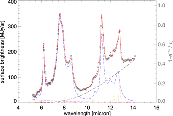
Figure 4. Isolating the different emission components from the 5.2–14.2 μm SL Spitzer-IRS spectrum (black crosses) of a position in M17. The propagated statistical uncertainties have been indicated for each resolution element and are typically smaller than the plot symbol. The dashed lines show the sum of each of the subcomponents, with the PAH emission in blue, the line emission in orange, the stellar contribution in purple, and the warm dust contribution in black. The solid red line shows their summed spectrum. The extinction assumes a mixed model and the Galactic center extinction curve from Chiar & Tielens (2006). Note that they found a visual extinction  . See Section 3.1 for details.
Download figure:
Standard image High-resolution imageThe molecular hydrogen and atomic emission lines with a signal-to-noise ratio greater than 2 are subsequently removed from the spectra by linearly interpolating across the feature's instrumental width. If present, the  S(2) and/or [Ne ii] emission lines are treated differently, as they are heavily blended with the 12.7 μm PAH band at the resolution of the IRS's SL module. Separating these lines from the PAH feature follows the approach described by Shannon et al. (2015), in which an emission-line-free 12.7 μm PAH band is used as a template to fit the feature in the other spectra. Here an emission-line-free 12.7 μm PAH band from NGC 7023 is used for all targets. The fitting region is selected such that it excludes resolution elements affected by the emission lines. In the case of a strong [Ne ii] emission line, the entire 12.7 μm PAH band is replaced with the entire scaled template profile. In cases where there is only H2 emission, the resolution elements of the H2 (S2) line are only replaced with those from the scaled template profile. Shannon et al. (2015) reported that this method is highly reliable, with an error of no more than 2%–3%. Lastly, the complete PAH emission spectrum is isolated by correcting for extinction and subtracting the continuum.
3.2. Fitting the PAH Emission Spectrum
The database-fitting approach follows that outlined in BBA16, with some adjustments and enhancements. Fitting an astronomical spectrum is a two-step process. First, density functional theory (DFT)–computed absorption spectra from PAHdb's libraries are converted into PAH emission spectra. Second, these modeled emission spectra are used to actually fit the observed astronomical PAH emission spectra. A brief overview of the approach taken in modeling the PAH emission process and the utilized fitting technique follows.
3.2.1. Converting PAH Absorption Spectra into PAH Emission Spectra
Band shift. Since the astronomical emission spectra originate in highly vibrationally excited molecules, anharmonic effects induce a small redshift to the emission band peak positions relative to the band positions measured in absorption. Here a 15 cm−1 redshift is taken, a value consistent with the average of the shifts measured in a number of experimental mid-IR studies of emission spectra from highly vibrational excited PAHs and absorption spectra of PAHs measured at high temperatures (Cherchneff & Barker 1989; Flickinger et al. 1990; Brenner & Barker 1992; Colangeli et al. 1992; Joblin et al. 1995; Williams & Leone 1995; Cook & Saykally 1998).
Band profile. The intrinsic emission profile for a single, unperturbed vibrational transition is Lorentzian. However, the observed astronomical bands form from a blend of Lorentzian bands with different centroids and widths (e.g., Pech et al. 2002). Assuming that these are statistically distributed, as in BBA13 and BBA16, Gaussian band profiles are used. A FWHM of 10, 15, and 20 cm−1 for bands falling longward of 15, between 10 and 15, and shortward of 10 μm are chosen, respectively. These FWHM values reflect the bandwidth variations observed in astronomical spectra (e.g., Peeters et al. 2002; van Diedenhoven et al. 2004).
Excitation/emission process. When considering the emission spectrum from a highly vibrationally excited individual PAH, the relative band intensities depend on PAH size and excitation energy. The overall excitation/emission process is modeled using the thermal approximation (e.g., Schutte et al. 1993; Verstraete et al. 2001). Since PAH excitation is driven by the absorption of UV photons in most astronomical objects, the excitation model incorporates (1) the size-dependent cross section for each PAH described by Draine & Li (2007) and (2) the energy range of the incident radiation field described by a stellar atmosphere model from the Atlas9 Stellar Atmosphere Models (Castelli & Kurucz 2004) at the effective stellar temperature of the irradiating star (see Table 1). Note that metallicity is taken as solar and surface gravity  for all stars. The emission model considers the different maximum excitation temperature each PAH achieves based on its heat capacity and computes the emission, taking the full vibrational cascade into account as the PAH relaxes stepwise down the vibrational ladder from the highest excitation level to the vibrational ground state (see also Bauschlicher et al. 2010; Boersma et al. 2010 and references therein).
3.2.2. Fitting Astronomical PAH Spectra
Fitting technique. Spectroscopic fitting is performed using a nonnegative least-squares (NNLS) algorithm (Lawson & Hanson 1974) that has been adapted to minimize the  (non-negative least-Chi-squares, NNLC; Désesquelles et al. 2009). Note that the plateaus underlying the distinct PAH features are included for the fit, and, due to the limited spectral resolution of the SL module, it is not necessary to resample the emission onto a uniformly sampled frequency grid, as was needed in BBA13.
The database analyses are performed using version 2.00 of the library of computed spectra and the AmesPAHdbIDLSuite2 (dated 2015 August 27; Bauschlicher et al. 2010; Boersma et al. 2014a) from PAHdb. It is the AmesPAHdbIDLSuite suite of IDL3 -object classes that interacts with the spectral library, applies the PAH emission model to convert the absorption data into emission spectra, implements the NNLC fitting algorithm to fit each astronomical emission spectrum with the computed emission spectra, and does the bookkeeping for breaking the emission down into contributing PAH subclasses, e.g., charge and size. The database-fitting approach is illustrated in Figure 5, where the same spectrum of M17 shown in Figure 4 is broken down by PAH charge. The figure shows that the overall fit to the observed spectrum is good.

Figure 5. The PAHdb fit (solid black line) to the same 5.2–14.2 μm SL Spitzer-IRS spectrum (dashed gray line) from M17 as shown in Figure 4, corrected for extinction. The propagated statistical uncertainties are indicated for each resolution element. The dashed black line shows the determined continuum. The PAH spectrum is broken down according to charge, i.e., into emission originating from PAH anions (red), neutrals (green), and cations (blue). See Section 3.2 for details.
Download figure:
Standard image High-resolution imageFigure 6 presents three-color composite images for each of the targets representing charge and size, constructed from the PAHdb breakdown described above. One thing to keep in mind is that the anion contribution in the charge breakdown image is likely overestimated due to the overlap of the red wing arising from the anharmonic redshift with the possible anion contribution (red channel), which consistently falls to the red of the main PAH band (see also Section 5.6). For PAH size, a nonuniform histogram with three bins is constructed, binning the absolute contribution from PAHs with effective radii between 0 and 6.5 Å ( ), small; 6.5–10 Å (
 ), large; and 10–12 Å (
 ), very large. These correspond to the red, green, and blue channels, respectively. The effective radius (
 ), in Å, is calculated as
where A is the total area of the PAH in Å2, calculated from counting the number of three to eight–membered rings (ni) and multiplying that number by the area of an individual ring, i.e.,

Figure 6. Three-color composite images constructed from the PAHdb charge and size breakdown results. For charge (top), the absolute contribution from anionic, neutral, and cationic PAHs are shown in red, green, and blue, respectively. For size (bottom), the absolute contribution from PAHs with an effective radius of 0–6.5, 6.5–10, and 10–12 Å (small, large, and very large) are shown in red, green, and blue, respectively. See Table 2 for examples of PAHs in each size bin. Left: RN NGC 7023. Middle: H ii region M17. Right: PN NGC 40. The pixel size is indicated by the labeled box, and the star/arrow shows the position of/points toward the irradiating source. The pixel values associated with each channel (red, green, and blue) have been linearly scaled to cover the channel's entire dynamic range (i.e., 8 bit; 0–255), with a 1% cutoff on both the high and low end of the normalized cumulative distribution of pixel values. The latter helps suppress any outliers. See Section 3.2 for details.
Download figure:
Standard image High-resolution imageTable 2 provides a few examples of PAHs and their effective radii.
Table 2. Eight PAHs and Their Effective Radii from Equations (1) and (2)
| Formula | Size Bin | Structure | Radius (Å) |
|---|---|---|---|
| C20H12 | s |

|
2.75 |
| C24H12 | s |

|
3.37 |
| C32H14 | s |

|
4.03 |
| C66H20 | s |

|
6.25 |
| C96H24 | L |

|
7.74 |
| C112H26 | L |

|
8.44 |
| C150H30 | L |

|
9.94 |
| C190H34 | VL |

|
11.3 |
Note. s: small; L: Large; VL: very large.
Download table as: ASCIITypeset image
3.3. Determining PAH Band Strengths
The literature provides several "traditional" approaches to separate the PAH bands from the underlying continuum and their plateaus (e.g., Sellgren et al. 2007; Smith et al. 2007b). The approach adopted here is based on that described in van Kerckhoven et al. (2000), Hony et al. (2001), Peeters et al. (2002), and van Diedenhoven et al. (2004). Given the sizable amount of data, this procedure has been automated using a stiff ( ) spline continuum, as demonstrated in Figure 7. Here anchor points are chosen at the minima within a five-element search window surrounding fixed positions between the observed features to isolate the 6.2, "7.7," 11.2, 12.0, 12.7, 13.5, and 14.2 μm PAH bands. Note that the 6.0 and 11.0 μm satellite features are included when isolating the 6.2 and 11.2 μm PAH bands, respectively. At the resolution of the SL data, these satellite features are heavily blended with the main features. The "7.7" μm complex was further decomposed by fitting a second-order polynomial between points near 8.0 and 9.0 μm, allowing extraction of the 8.6 μm PAH band. The 7.6 and 7.8 μm components were separated by integrating the emission falling shortward and longward of 7.72 μm for the 7.6 and 7.8 μm PAH bands, respectively. It is noted that, compared to BBA16, an additional anchor point has been introduced at 10.7 μm to avoid the continuum cutting off part of the 11.2 μm PAH band in spectra with a strong 10–15 μm plateau, notably for NGC 40.

Figure 7. Isolating and measuring the strengths of the PAH emission bands in the same 5.2–14.2 μm SL Spitzer-IRS spectrum from M17 as shown in Figures 4 and 5, corrected for extinction, continuum subtracted, and with emission lines removed. The propagated statistical uncertainties have been indicated for each resolution element and are typically smaller than the plot symbol ("+"). The solid black line shows the spline continuum used to isolate the PAH bands, together with their anchor points ("+") in red. The isolated PAH bands, after subtracting the spline continuum, are shown underneath the spectrum with solid lines, each band colored separately. Note the separation of the three components of the "7.7" μm PAH band complex, i.e., the 7.6, 7.8, and 8.6 μm PAH features. See Section 3.3 for details.
Download figure:
Standard image High-resolution imageThe analysis is performed on the extinction-corrected, emission line–removed, and continuum-subtracted spectra from Section 3.2. Uncertainties have been statistically propagated. While determination of the spline continuum will have added to the uncertainty, this should be small and systematic for the high-quality data. Thus, continuum subtraction should not significantly affect differences and ratios. Indeed, several studies have now established that PAH band trends are mostly independent of the way the bands are traditionally isolated (e.g., Galliano et al. 2008; Peeters et al. 2012).
3.4. Calibrating the Qualitative Charge Proxies
PAH band strength ratios between bands in the 6–15 μm region have long been used as qualitative proxies to track variations in the properties of the emitting PAH population, e.g., charge and structure. Comparing the behavior of these ratios with the ratio determined from the database-fitting approach allows one to quantitatively calibrate these proxies.
Most commonly, the 6.2 μm PAH band is used as a proxy for PAH cations, while the 11.2 μm PAH band is used as a proxy for neutral PAHs, i.e.,

where  and
and  are the PAH cation and neutral densities determined using PAHdb, respectively, and
  and
and  are the 6.2 and 11.2 μm PAH band strengths, respectively. Figure 5 shows that these proxies are not quantitative by themselves, as PAHs in all three charge states contribute to each band. Nonetheless, they have proven to be generally reliable tracers for the charge state of the PAH population (e.g., Hony et al. 2001; Peeters et al. 2002; Bregman & Temi 2005; Compiègne et al. 2007; Galliano et al. 2008; BBA16).
Figure 8 presents the traditionally determined 6.2/11.2 μm PAH band strength ratio map for each of the targets, and the top panels in Figure 9 show the corresponding  ratio map, where
  and
and  are directly taken from the PAHdb charge decomposition. The bottom panels in Figure 9 show the PAHdb-determined large fractional size (
 /(
/( +
+  )) contribution maps. The black line in Figure 10 traces the PAH charge, and the orange line traces the PAH size changes along the line shown in Figure 3.

Figure 8. The 6.2/11.2 μm PAH band strength ratio map for each target commonly used as a qualitative proxy for PAH charge. Note that the color range in all maps has been set such that it covers 98% of the pixel values. That is, there is a 1% cutoff on both the high and low end of the normalized cumulative distribution of pixel values. This helps suppress any outliers. See Section 3.4 for details.
Download figure:
Standard image High-resolution image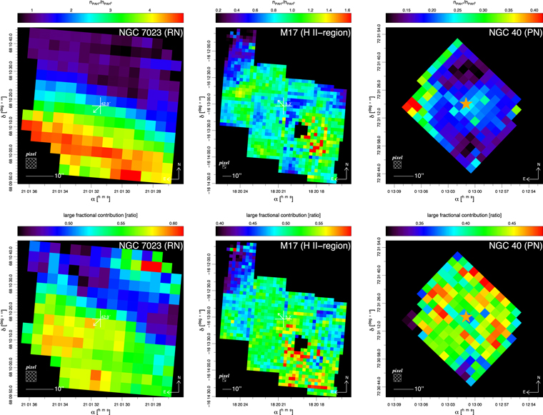
Figure 9. The PAHdb-determined  ratio (top row) and large PAH fractional contribution (
 /(
/( ); bottom row) maps for each target. Note that the color range in all maps has been set such that it covers 98% of the pixel values. That is, there is a 1% cutoff on both the high and low end of the normalized cumulative distribution of pixel values. This helps suppress any outliers. See Section 3.4 for details.
Download figure:
Standard image High-resolution image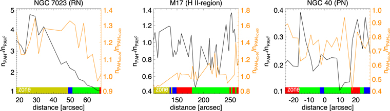
Figure 10. Traces of the  ratio (charge; black line) and
  ratio (size; orange line) PAHdb breakdown along the line shown in Figure 3 across each of the targets. The distance is from the dominating irradiating source, and the color bar is coded according to each data point's associated zone in Figure 3. See Section 3.4 for details.
Download figure:
Standard image High-resolution imageKnowledge of the charge state of the PAH population can be directly related to the physical conditions in the local environment through the PAH ionization parameter (Bregman & Temi 2005; Galliano et al. 2008; Fleming et al. 2010; BBA15; BBA16; Stock et al. 2016). The PAH ionization parameter is defined as  , where G0 is the strength of the radiation field in terms of the Habing field (Habing 1968;
  erg cm−2 s−1),
  is the gas temperature (in K), and ne is the electron density (in cm−3).
When assuming only two accessible ionization states and parameters applicable for circumcoronene4
(C54H12), which is considered representative for an average interstellar PAH ( ; e.g., Croiset et al. 2016), the PAH ionization parameter can be expressed as (see Boersma et al. 2014a)

The reasons for only considering two PAH ionization states (PAH , PAH
, PAH ) is due to the unreliability associated with determining the anion contribution. In Section 5.6, among other things, the quantification of the PAH charge is further discussed.
3.5. Analyzing the Molecular Hydrogen Bands
Figure 2 clearly shows pure rotational  lines present in spectra of NGC 7023 and M17. Following an approach comparable to that outlined by Fleming et al. (2010), the pure rotational
  lines are utilized to determine the gas temperature (
 ), H2 column density (
 ), and H2 ortho-to-para ratio (
 ). The
  molecular parameters were obtained from the HITRAN Database (Rothman et al. 2013). Here
  ,
,  , and
, and  are determined by minimizing the Euclidean distance norm between observations and model obtained from fitting a straight line with parameters
  and
and  while iterating on
  . At least three
  lines with a signal-to-noise ratio greater than three are required for a pixel to be evaluated. In addition,
  is forced strictly positive and needs to converge and not exceed three. Figure 11 demonstrates the approach by showing the population diagram constructed from the
  lines present in a 5.2–14.2 μm SL Spitzer-IRS spectrum from M17 near the location of the spectrum shown in Figures 4, 5, and 7. Note that the
  lines are corrected for extinction, and uncertainties are propagated. Figure 12 presents maps of
  and
and  for each target. Due to the lack of any apparent morphological substructure, the ortho-to-para-ratio maps have been omitted from the figure and are not further discussed. The reader is directed to Fleming et al. (2010) for a more detailed analysis and discussion of the
  ortho-to-para-ratio across NGC 7023.
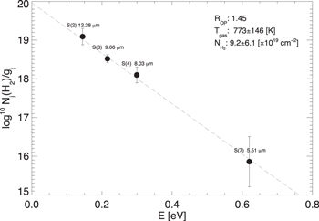
Figure 11. Pure rotational  population diagram analysis of a 5.2–14.2 μm SL Spitzer-IRS spectrum from M17 close to the position of the spectrum shown in Figures 4, 5, and 7, corrected for extinction. The propagated statistical uncertainties have been indicated. The dashed gray line shows the best fit, and the best-fit parameters are given with their uncertainties. See Section 3.5 for details.
Download figure:
Standard image High-resolution image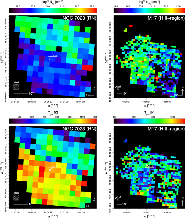
Figure 12. The H2 column density ( top) and gas temperature (
 bottom) determined from the pure vibrational
  population diagram analyses for NGC 7023 and M17. Note that the color range in all maps has been set so that it covers 98% of the pixel values. That is, there is a 1% cutoff on both the high and low end of the normalized cumulative distribution of pixel values. This helps suppress any outliers. See Section 3.5 for details.
Download figure:
Standard image High-resolution image4. Results
The results are presented in two subsections. The first presents results on the state of the PAH population in each target; the second presents results derived from the pure rotational  population diagram analyses.
4.1. The State of the PAH Population
Results on the state of the PAH population are presented for PAH charge and size, looking at both the morphologies present in the different maps and possible PAH proxy calibrations.
4.2. PAH Charge
The morphological structure of the PAH charge distribution across each target is shown in Figure 6, Figure 8, the top row of panels in Figure 9, and in Figure 10. Figure 6 captures the charge variations across each target using a three-color composite image, where the red, green, and blue channels depict the contribution from PAH anions, neutrals, and cations, respectively. The figure shows a morphological structure in good agreement with that present in Figure 1 for each target. That is, for NGC 7023, there is a clear delineation between the dense and diffuse medium to the north and south of the PDR, respectively, with emission from neutral PAHs peaking in the denser northwest region. Similar behavior holds for M17, where the "bright" and "dark" regions fall to the northeast and southwest, respectively, with emission from neutral PAHs peaking in the northeast. For NGC 40, the emission intensity peaks in the ring surrounding the central white dwarf. While Figure 6 does not apply a normalization, Figure 8 does, thus avoiding any morphological features simply appearing due to a more-is-more type of behavior. Figure 8 uses the 6.2/11.2 μm PAH band strength ratio as a proxy for the PAH charge. For NGC 7023, the ratio shows a gradual decrease when moving away from the irradiating star. However, the "ring" visible in Figures 1 and 6 is absent here. The striking feature in the 6.2/11.2 μm PAH band strength ratio map of M17 is the "hot spot" located slightly northeast of the center of the map. Apart from the obvious circular symmetry around the central star, NGC 40 does not show much substructure in its 6.2/11.2 μm PAH band strength ratio map. Overall, the measured ratios are low—perhaps the ratio peaks off the bright "ring" visible in Figures 1 and 6. Figure 9 uses the PAHdb-determined  ratio to track the PAH charge morphology across each target. For NGC 7023, there is a general decrease in the ratio when moving away from the irradiating source, and the maps shown in Figures 8 and 9 are very comparable. For M17, the "hot spot" present in Figure 8 is absent in Figure 9. However, a smaller, less bright "hot spot" appears slightly offset to the east of the one present in Figure 8. For NGC 40, the morphology in Figure 9 shows a uniform brightening at the northeastern edge of the region that is choppy in Figure 8. However, the interior regions show more morphological agreement between the two figures. Finally, Figure 10 traces the
  ratio along the lines shown in Figure 3 and provides a one-dimensional view of the PAH charge variations across each target as a function of distance from the irradiating source. Although the (somewhat noisy) trace across M17 does not show significant variation, the traces for NGC 7023 and NGC 40 do. For NGC 7023, the
  ratio jumps from ∼0.5–0.6 in the vicinity of the exciting star to ∼0.9 some 25'' from HD 200775. The ratio remains at about 0.8 across the diffuse region until it crosses the PDR, where it starts a steady decline as it moves further into the dense region. For NGC 40, the behavior of the
  ratio across the nebula clearly reflects a spherical morphology. It is symmetric with respect to the exciting star, peaking at the edge of the ring to ∼0.8–0.9, dropping between the exciting star and ring to ∼0.1–0.3, and rising to 0.4 as it crosses the Wolf–Rayet star at its center.
Moving away from morphology, all of the data from Figures 8 and 9 are combined to quantitatively calibrate the 6.2/11.2 μm PAH band strength ratio with the PAHdb-determined  ratio and the PAH ionization parameter
  . This calibration is done in Figure 13. The figure shows that the dynamic range in abscissa values is dominated by NGC 7023, which shows a reasonably good correlation with the 6.2/11.2 μm PAH band strength ratio. NGC 40 lines up well with NGC 7023, albeit only occupying low ordinate and abscissa values. M17 also follows the overall trend with a slightly larger range in abscissa values compared to NGC 40 and a coagulation of points along a vertical line around
 ![${G}_{0}{T}^{1/2}/{n}_{{\rm{e}}}\ [\times {10}^{4}\ {\mathrm{cm}}^{3}]$](https://content.cld.iop.org/journals/0004-637X/858/2/67/revision1/apjaabcbeieqn81.gif) of about three. The poor squared linear correlation coefficient (
of about three. The poor squared linear correlation coefficient ( ) is mostly due to M17, as its number of data points exceeds that on NGC 7023 and NGC 40 combined by almost a factor of five. Omitting the M17 data yields a linear correlation coefficient of
  .
.
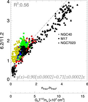
Figure 13. The 6.2/11.2 μm PAH band strength ratio charge proxy plotted vs. the database-determined  ratio and the inferred PAH ionization parameter
  . Note that
  is simply obtained by multiplying the
  ratio with 2.66; cf. Equation (4). Each symbol represents a different target, and for M17, each data point has been color-coded according to its associated zone, as given in Figure 3. The linear best-fit equations (weighted) and the squared linear relation coefficients (weighted;
  short-dashed lines) are also given. See Section 4.2 for details.
Download figure:
Standard image High-resolution imageIn BBA15 and BBA16, the 8.6/11.2 μm PAH band strength ratio was shown to be very useful as a proxy for the PAH charge. Plotting the 8.6 versus 11.2 PAH band strength for NGC 7023 resulted in a bifurcated plot establishing two well-defined limiting lines: one associated with the dense medium, the other with the diffuse medium (BBA14). Figure 14 presents these relationships for the targets studied here. The left panel of the figure shows an overall good trend of the  ratio with the 8.6/11.2 μm PAH band strength ratio, where the range in the
  ratio is dominated by NGC 7023. Compared to the 6.2/11.2 μm PAH band strength ratio shown in Figure 13, both M17 and NGC 40 are more in line with the established trend. The somewhat poor squared linear relation coefficient (
 ) is again due to M17 dominating the coefficient because of its large number of data points when compared to the other two targets.

Figure 14. The 8.6/11.2 μm PAH band strength ratio established as a proxy for PAH charge (left) and a calibrated measure of the PAH  ratio (right). Left: the linear best-fit equations (weighted) and squared linear relation coefficients (unweighted;
  short-dashed lines) are also given. Right: the 8.6 vs. 11.2 μm PAH band strength calibrated for the PAH
  ratio. The data on NGC 7023, M17, and NGC 40 fall in the purple, green, and red shaded areas, respectively. Note that for M17 and NGC 40, the ordinate and abscissa values were both multiplied with a constant factor to put them in the range set by NGC 7023. See Section 4.2 for details.
Download figure:
Standard image High-resolution imageThe right panel in Figure 14 presents the 8.6/11.2 μm PAH band diagnostic template, where the data on M17 and NGC 40 have been scaled into the domain of NGC 7023 by multiplying both the ordinate and abscissa with a constant factor, i.e., preserving the slope and therefore their associated 8.6/11.2 μm PAH band strength ratio and  ratio. Overplotted are lines with a constant
  ratio. The figure shows that all of the M17 data (green shaded area) fall inside the space occupied by that of NGC 7023 (purple shaded area), while little of the NGC 40 data (red shaded area) overlaps with that of M17 or NGC 7023. The bulk of the NGC 40 data extends toward and abuts the
  limit.
4.2.1. PAH Size
The lower panels in Figure 6 capture the morphological structure of the PAH size variations across each of the targets considered here using a three-color composite image, where the red, blue, and green channels depict the contribution from PAHs in the three nonuniform size bins of effective radii in the ranges 0–6.5, 6.5–10, and 10–12 Å. As with the PAH charge, there is good agreement with the morphological structure apparent in this figure and that presented in Figure 1. For NGC 7023, there is a clear segregation between the dense and diffuse medium to the northwest and southeast of the PDR, respectively, with the 6.5–10 Å size bin peaking in the latter region. In addition, the "bright" ring extruding from the PDR is clearly visible. The image for M17 shows the same divide between the "dark" and "bright" region as its charge counterpart. In the case of NGC 40, the size bins peak in the ring surrounding the central Wolf–Rayet star. The orange line in Figure 7 traces the  ratio across the lines shown in Figure 3 as a function of distance from the irradiating source. For NGC 7023, from the irradiating source out, there is no change in the
  ratio until crossing the PDR (at ∼50''), where it starts to decline rapidly. No clear trends can be discerned for the somewhat noisy traces of M17 and NGC 40.
The PAH size has traditionally been probed by the 3.3/11.2 μm PAH band strength ratio proxy because emission in both bands originates in CH vibrational modes and the smallest members of the emitting PAH population dominate the emission at 3.3 μm while the larger members of the PAH family dominate the emission at 11.2 μm (e.g., Cohen et al. 1985). This is because, for a fixed excitation energy, the energy distribution across the different vibrational modes decreases as the PAH molecular size increases. Thus, the larger the PAH, the less probable the emission from higher-frequency modes. However, due to the lack of Spitzer-IRS spectra covering the 3.3 μm PAH band, calibration of the 3/11.2 μm PAH band strength ratio as a quantitative proxy for PAH size is not possible. While it is possible to combine our data with those taken from other observatories, e.g., SOFIA (Croiset et al. 2016), that is beyond the scope of this paper. However, a comparison between the results found here for the PAH size evolution across NGC 7023 and those found by Croiset et al. (2016) is discussed in Section 5.1.
4.3. H2-derived Parameters
From the pure rotational  lines present in the spectra, the ortho-to-para ratio, molecular hydrogen density, and gas temperature for NGC 7023 and M17 were derived from fits to population diagrams such as that presented in Figure 11. One thing to note in that figure is that the reported uncertainty for
  is high, which is not immediately expected when looking at the figure. The large uncertainty comes from propagating the uncertainty on
  (=19.96;
  ), which is what is established by fitting the dashed straight line through the three data points shown in Figure 11. With x as
  , the propagated uncertainty is given by

which equates to the reported  cm−2.
cm−2.
Figure 12 shows that the molecular hydrogen density ranges from about 19.75 to 22.6 and 19.5 to 22.2 for NGC 7023 and M17, respectively. The temperature of the gas ranges from about 450 to 1100 and 400 to 1100 K for NGC 7023 and M17, respectively. Both the molecular hydrogen density and temperature maps for NGC 7023 show a clear separation across the PDR boundary, with higher densities and cooler temperatures to the north of the PDR. The M17 map for the molecular hydrogen density shows no real substructure. The map for the gas temperature does not either; however, the color scaling seems dominated by a few hot spots.
5. Discussion
The results are discussed in six subsections. The first considers the PAH size evolution across NGC 7023, the second the charge balance and calibration, the third the spectroscopic templates (principal components) used to reproduce the observed spectra, the fourth the H2-derived parameters, the fifth the role of the adopted extinction curve, and the sixth some final thoughts.
5.1. PAH Size Evolution across NGC 7023
Croiset et al. (2016) traced the PAH size evolution in NGC 7023 along a line comparable to that shown in Figure 3. The top frame of their Figure 6 shows an overall steady increase in the 11.2/3.3 μm PAH band strength ratio from 2 to 3 with distance from the exciting star almost all the way to the PDR boundary. There it sharply drops and quickly recovers when moving across the brightest spot in the PDR. Arguably, the noisy and far less well spatially sampled orange trace in Figure 10 shows, in broad strokes, similar behavior for the  ratio, with a small increase in the ratio from 1.2 to 1.3 with distance from HD 220775 up to the PDR interface (∼51''), where it sharply drops. However, the ratio fails to recover when moving deeper into the molecular cloud. However, it should be noted that the trace in Figure 10 extends some 20'' further into the molecular cloud and actually does not capture the brightest spot in the PDR, and, given the poor spatial sampling, it could well be that the sharp drop and its subsequent recovery are captured in a single pixel.
5.2. The PAH Charge Balance
The PAH charge distribution is discussed in terms of the morphology of the targeted regions and the quantitative calibration of the PAH band strength ratio proxies with the PAHdb-determined charge breakdown.
5.2.1. The Morphology
NGC 7023. The morphological structure bordering the northwest PDR in NGC 7023, in terms of the PAH charge, shows a clear separation across the PDR boundary with, as expected, the PAH population showing a gradually decreasing degree of ionization when moving away from the irradiating source. These results are in agreement with those presented in other work, e.g., Fleming et al. (2010), Pilleri et al. (2012), BBA13, and BBA16. When crossing from the PDR into the denser, molecular domain, the increasing density attenuates the ionizing radiation from HD 200775 and provides more recombination opportunities.
M17. The morphology of M17, in terms of PAH charge, has two features that stand out. The first is the separation between the neutral region in the northeast, associated with zone 4 (Figure 3), and a more ionized region to the southwest. However, this distinction is not as strong as in NGC 7023 and seems counterintuitive, having a somewhat higher degree of ionization present further away from CEN1, the exciting star. Also, the separation is loosely associated with the "bright" and "dark" regions apparent in Figure 1. The second feature, which is only seen when looking at the 6.2/11.2 μm PAH band strength ratio map (Figure 8), is the curious "hot spot" situated near the intersection of the "bright" and "dark" regions in Figure 1. The absence of this "hot spot" in Figure 9 could be due to the PAHdb fitting procedure compensating for the large 6.2/11.2 μm PAH band strength ratio by some other means than a large  ratio. Indeed, PAHdb breakdown plots such as that presented in Figure 5 show that the 6.2 μm band contains contributions from neutral PAHs as well. Furthermore, inspection of the PAH anion breakdown map reveals that the PAH anion contribution is consistently low at the "hot spot," which, in turn, indicates that the large 6.2/11.2 μm PAH band strength ratio is due to a relatively weak 11.2 μm PAH band strength because of an absent red wing. Unfortunately, the trace in Figure 10 crossing M17 along the line depicted in Figure 3 does not capture either of these two features, as the figure depicts the
  ratio—which does not show the "hot spot"—and it samples zone 4 only sparsely. The study by Yamagishi et al. (2016) on M17 also identifies the "hot spot," but the separation from adjacent areas is less distinct in their 6.2/11.3 μm PAH band strength ratio map. These authors conclude that the degree of ionization is largely controlled by local physical conditions rather than the UV field from CEN1, perhaps by obscured B-type—or later—stars.
NGC 40. Any morphological substructure in the PAH charge maps for NGC 40 is, at best, tentative. While the ringlike structure of the PAH emission is clearly apparent in the intensity/density-driven three-color composite PAHdb charge breakdown map of Figure 6, it is far more difficult to discern in the 6.2/11.2 μm PAH band strength ratio map of Figure 8 and the  ratio map of Figure 9. For one, the structure in the maps seems largely dominated by a few outliers. The dynamic range of PAH charge indicators covers about a factor of 3–4, which is comparable to those observed for NGC 7023 and M17. Nonetheless, they are at a considerably lower absolute value for NGC 40. Possibly high internal attenuation—measured here as
  —explains the low degree of ionization seen.
5.2.2. The PAH Charge Proxy Calibrations
The calibration of the 6.2/11.2 μm PAH band strength ratio with the PAHdb-determined  ratio and, subsequently, the PAH ionization parameter
  in Figure 13 is, to a large degree, linear, with a vertical excursion for some of the data points associated with M17. These outlying data points are traced back to the "hot spot" in the proxy band results shown in Figure 8, which is absent in the PAHdb-based analysis in Figure 9. The dynamic range for the ionization parameter, which is almost entirely determined by NGC 7023, is somewhat smaller than that established in BBA16 and does not show the curvature observed in that work. The 6.2/11.2 μm PAH band strength ratios determined in BBA16 for the RN NGC 7023 are considerably larger compared to those measured here (∼0.9–2.9 versus ∼0.9–3.9), which is traced back to how the 11.2 μm PAH band has been isolated. This work uses an additional anchor point that effectively leaves less emission in the 11.2 μm PAH band and thus increases the 6.2/11.2 μm PAH band strength ratio. Second, a somewhat different approach in isolating the continuum and how that interplays with the extinction correction (see Section 5.5) results in slightly different isolated PAH spectra. Subsequent spectroscopic fitting in BBA16 and here yields for NGC 7023 a maximum ionized fraction of 84% versus 88%, translating into an
  ratio of 5.2 versus 7.3 and
  equal to 14 versus 19
 ![$[\times {10}^{4}\,{\mathrm{cm}}^{3}]$](https://content.cld.iop.org/journals/0004-637X/858/2/67/revision1/apjaabcbeieqn115.gif) , respectively. The calibration of the 6.2/11.2 μm PAH band strength ratio with the PAH ionization parameter done here differs from that reported in Galliano et al. (2008) and Stock et al. (2016), including when using the approach set out by Fleming et al. (2010). The main driver of these differences is the considerably larger 6.2/11.2 μm PAH band strength ratios arrived at in this work. To reiterate, the reason for these larger 6.2/11.2 μm PAH band strength ratios is the systematically lower 11.2 μm PAH band strength determined here because of the additional anchor point at 10.7 μm used to better isolate the band; see Section 3.3. Overall, differences in instrumentation, spectral resolution, and method for determining the continuum between observations can have a significant impact on the measured PAH band strengths. Nonetheless, it has been shown that established trends typically hold when keeping these variables constant, e.g., Galliano et al. (2008), Peeters et al. (2012), BBA15, Stock et al. (2016), and BBA16, which is again confirmed here.
, respectively. The calibration of the 6.2/11.2 μm PAH band strength ratio with the PAH ionization parameter done here differs from that reported in Galliano et al. (2008) and Stock et al. (2016), including when using the approach set out by Fleming et al. (2010). The main driver of these differences is the considerably larger 6.2/11.2 μm PAH band strength ratios arrived at in this work. To reiterate, the reason for these larger 6.2/11.2 μm PAH band strength ratios is the systematically lower 11.2 μm PAH band strength determined here because of the additional anchor point at 10.7 μm used to better isolate the band; see Section 3.3. Overall, differences in instrumentation, spectral resolution, and method for determining the continuum between observations can have a significant impact on the measured PAH band strengths. Nonetheless, it has been shown that established trends typically hold when keeping these variables constant, e.g., Galliano et al. (2008), Peeters et al. (2012), BBA15, Stock et al. (2016), and BBA16, which is again confirmed here.
The calibration of the 8.6/11.2 μm PAH band strength ratio with the  ratio in the left panel of Figure 14 does not show the vertical excursion present in Figure 13, which is based on the traditional 6.2/11.2 μm proxy for PAH charge. If the presence of the "hot spot" in M17 is indeed due to the absence of a pronounced red wing to the 11.2 μm PAH feature (see Section 5.2.1), this would suggest that the 8.6 μm PAH band is affected in a similar way as the 11.2 μm PAH band. Compared to BBA16, there is much less scatter in the calibration, which is likely related to some of the data used in BBA16 having substantially lower signal-to-noise.
Figure 14 shows that the data spread presented by M17 is entirely encompassed within the envelope set up by NGC 7023. On the other hand, the bulk of the data associated with NGC 40 is outside this envelope and bordering on the zero charge ratio limit. NGC 40 probes the PAH charge distribution at (very) low ionization fractions and shows a high degree of consistency with the relationships established from the moderately high ionization fractions extrapolated into the lower domain.
5.3. PAH Spectroscopic Templates
With the aim of developing diagnostic tools that are straightforward to use and that can be applied to all astronomical PAH spectra and to assess the presence of principal components (see, e.g., Berné et al. 2007; Pilleri et al. 2012), as discussed in BBA13 and BBA16, PAHdb template spectra for PAH charge and size have been derived. These template spectra are determined by normalizing the integrated flux for each of the PAH subclass spectra obtained from the database fit at each pixel to unity and taking the average for each target. The resulting five PAH subclass templates—i.e., three for PAH charge (anion, neutral, and cation) and two for size, large ( ) and small (
 )—are presented in Figure 15.5
Note that the templates are extended to cover the entire 2.5–20 μm wavelength range, while the fitted data cover only 5.2–14.2 μm. The figure shows that each of the PAH template spectra compares well for each different target. This is corroborated by Table 3, which presents the Pearson correlation coefficient between each of the template spectra derived for each target. The table shows that the template spectra derived from NGC 7023 match best with those derived from M17. In turn, those derived from NGC 40 match best with those derived from M17. However, the Pearson correlation coefficients between the template spectra derived in BBA16 for NGC 7023 and the RN NGC 2023—with coefficients of 0.99, 0.98, 1.00, 0.99, and 0.96 between their anion, neutral, cation, large, and small template spectra, respectively—surpass any of those reported here for NGC 7023.
)—are presented in Figure 15.5
Note that the templates are extended to cover the entire 2.5–20 μm wavelength range, while the fitted data cover only 5.2–14.2 μm. The figure shows that each of the PAH template spectra compares well for each different target. This is corroborated by Table 3, which presents the Pearson correlation coefficient between each of the template spectra derived for each target. The table shows that the template spectra derived from NGC 7023 match best with those derived from M17. In turn, those derived from NGC 40 match best with those derived from M17. However, the Pearson correlation coefficients between the template spectra derived in BBA16 for NGC 7023 and the RN NGC 2023—with coefficients of 0.99, 0.98, 1.00, 0.99, and 0.96 between their anion, neutral, cation, large, and small template spectra, respectively—surpass any of those reported here for NGC 7023.

Figure 15. Template (principal-component) spectra for PAH charge and size derived using the database-fitting approach, with the left, middle, and right panels corresponding to NGC 7023, M17, and NGC 40, respectively. The 1σ standard deviation is shown as a gray envelope. Each spectrum has been normalized to its peak cross section, and the shift in the 11.2 μm band, particularly noticeable for the different PAH charge template spectra, is highlighted by the dashed lines. See Section 5.3 for details.
Download figure:
Standard image High-resolution imageTable 3. Pearson Correlation Coefficient between the Template Spectra Derived for Charge and Size for Each Target
| Charge | Size | |||||||||
|---|---|---|---|---|---|---|---|---|---|---|
| M17 | NGC 40 | M17 | NGC 40 | |||||||
| Anion | Neutral | Cation | Anion | Neutral | Cation | Small | Large | Small | Large | |
| NGC 7023 | 0.97 | 0.93 | 0.97 | 0.90 | 0.83 | 0.77 | 0.88 | 0.97 | 0.60 | 0.86 |
| M17 | 0.96 | 0.97 | 0.84 | 0.88 | 0.93 | |||||
Download table as: ASCIITypeset image
The validity of the template spectra is evaluated by fitting each target with the template spectra for the charge derived for the northwest PDR in NGC 7023. Here the observed spectrum at each position is fitted as the weighted sum of the three individual NGC 7023 charge template spectra:

Figure 16 presents the  ratio, i.e., c/b ratio, maps recovered for each target.
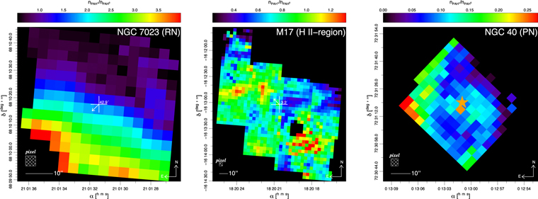
Figure 16. The  ratio as determined from the template fit decomposition for each target. Note that the color range in all maps has been set such that it covers 98% of the pixel values. That is, there is a 1% cutoff on both the high and low end of the normalized cumulative distribution of pixel values. This helps suppress any outliers. See Section 5.3 for details.
Download figure:
Standard image High-resolution imageFollowing Shannon et al. (2016), the Structural SIMilarity (SSIM) index is used to quantify morphological similarity between the  ratio maps determined from the template fit decomposition (i.e., Figure 16) and those from a direct database decomposition (i.e., Figure 9). The SSIM index is calculated on various windows, and for two images x and y, it is defined as (Wang et al. 2004)
where  and
and  are the average and variance of images x and y, respectively, and
  is their covariance. Here c1 and c2 are constants defined as
  and
and  , respectively. Here L is the dynamic range of the pixel values, i.e., 255 for an 8 bit image, and k1 and k2 are, respectively, by default 0.01 and 0.03. The convolution window is a 2D Gaussian with a width of 1.5 pixels, which is used for convolution. Two identical windows/images will have an SSIM index of 1. The original Matlab implementation6
from Wang et al. (2004) was ported to IDL7
and validated. It is noted that Shannon et al. (2016) utilized a uniform convolution window. Figure 17 presents the SSIM index maps and gives the averaged SSIM index. The figure shows that the results from the template fit and the direct database decomposition compare well for NGC 7023 and M17; NGC 40 fares far less well.
, respectively. Here L is the dynamic range of the pixel values, i.e., 255 for an 8 bit image, and k1 and k2 are, respectively, by default 0.01 and 0.03. The convolution window is a 2D Gaussian with a width of 1.5 pixels, which is used for convolution. Two identical windows/images will have an SSIM index of 1. The original Matlab implementation6
from Wang et al. (2004) was ported to IDL7
and validated. It is noted that Shannon et al. (2016) utilized a uniform convolution window. Figure 17 presents the SSIM index maps and gives the averaged SSIM index. The figure shows that the results from the template fit and the direct database decomposition compare well for NGC 7023 and M17; NGC 40 fares far less well.
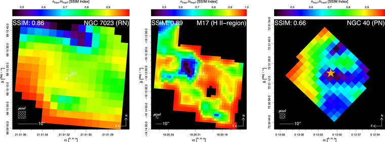
Figure 17. The SSIM maps comparing the  ratio determined from the template fit (principal component) decomposition (cf. Equation (6)) and from the direct database-fitting decomposition for each target. Indicated is the average SSIM index. Note that the color range in all maps has been set so that it covers 98% of the pixel values. That is, there is a 1% cutoff on both the high and low end of the normalized cumulative distribution of pixel values. This helps suppress any outliers. See Section 5.3 for details.
Download figure:
Standard image High-resolution imageFor M17, the "hot spot" seen in the 6.2/11.2 μm PAH band strength ratio map, which is absent in the  ratio map from the direct database decomposition, is reproduced by the template fitting, hence explaining the low SSIM index values near those positions in Figure 17.
While the template spectra for PAH charge derived from NGC 7023 produce overall acceptable fits, there are astronomical (local) environments in which they do not perform as well systematically. This could point to either a substantial difference in the underlying PAH population or that the ongoing changes to the PAH population are not well captured with variations in PAH charge alone.
5.4. H2-derived Parameters
The analyses of the  population diagrams provide insight into the
  density and gas temperature. A direct comparison of the results with those found by Fleming et al. (2010) on the northwest PDR in NGC 7023 show that the morphology of the molecular hydrogen density and temperature maps is in good agreement. For M17, many pixels did not meet the conditions set in Section 3.5 and have been left out of the maps. Possibly, the chosen extinction curve has a significant influence on these results (see Section 5.5).
Since the temperature of the gas ( shows up in the definition of the PAH ionization parameter (
 ), it can be used in a simple model to separately (from that outlined in Section 4.2) try to calibrate the 6.2/11.2 μm PAH band strength ratio. The strength of the radiation field (G0) is modeled by taking a blackbody at the effective temperature of the irradiating star, diluting it with the stellar radius over the projected distance squared, and integrating it from 91.2 to 111 nm. Determining the electron density (
 ) is far less straightforward, and therefore
  cm−3 is taken. This value is more or less consistent with that at the PDR in NGC 7023 (
 cm−3) when taking the total gas density as 4 × 103 cm−3 (Chokshi et al. 1988), assuming all free electrons come from C ii, and using the diffuse ISM gas-phase carbon abundance of
  (Cardelli et al. 1996). Figure 18 presents the results. The figure shows broad-stroke similarities with Figure 13; that is, the PAH ionization parameter values are of similar magnitude, and the dynamic range is determined by NGC 7023. However, Figure 13 shows a much tighter relation, and, specifically for M17, each zone is much more coherent. The most likely reason for this is that the electron density is probably not the same and constant across each target and that using the projected distance is not sufficient to capture the actual morphological details of the region.
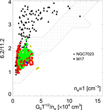
Figure 18. The 6.2/11.2 μm band strength ratio PAH charge proxy vs. the PAH ionization parameter ( ), with the strength of the radiation field (G0) determined from modeling the irradiating star as a blackbody, the gas temperature (
 ) determined from
  population diagrams, and the electron density (
 ) fixed at 1 cm−3. Each symbol represents a different target, and for M17, each zone has been color-coded according to its associated zone in Figure 3. The hatched region indicates where the calibration falls when doing the PAHdb analysis; cf. Figure 13. See Section 5.4 for details.
Download figure:
Standard image High-resolution image5.5. The Role of the Extinction Curve
The results and their interpretation are based on extinction-corrected data. The amount and spectral shape of this correction is highly dependent on the adopted extinction model (e.g., mixed versus screen), the shape of the used extinction curve, and its interplay with other components of the spectra (i.e., continuum, emission lines, etc.). Figure 19 compares the wavelength-dependent dilution factor derived from the three extinction curves considered here when assuming a mixed model (cf. Section 3.1) and a visual extinction AV of 19, translating to  in the case of the extinction curve toward the Galactic center from Chiar & Tielens (2006). The figure shows that there is a difference in the amount of actual extinction for the same AV. While this is significant when comparing the extinction curve from Chiar & Tielens (2006) with those from Weingartner & Draine (2001), the biggest impact on any results presented here and their subsequent interpretation would come from differences in spectral shape, since they heavily rely on PAH band strength ratios.
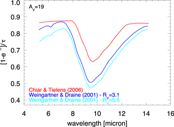
Figure 19. Comparison of the wavelength-dependent dilution factor  due to extinction between 5.2 and 14.2 μm for three extinction curves at a visual extinction
  . See Section 5.5 for details.
Download figure:
Standard image High-resolution imageWhile the spectral shape of the core silicate absorption feature centered around 9.7 μm is practically identical between ∼8 and 12 μm, the features from Weingartner & Draine (2001) continue to broaden where the profile from Chiar & Tielens (2006) levels out. From Weingartner & Draine (2001), the  extinction curve shows relatively more extinction at shorter wavelengths compared to the
  curve. From this, it is easily inferred that the choice of extinction curve can have a significant impact on the determined 6.2/11.2 μm PAH band strength ratio. Also, the strong interplay of the chosen extinction curve with the other components of the spectra proved to be, in some cases, highly unpredictable. Notably for M17, there appears to be a degeneracy between the arrived at total visual extinction (AV) and continuum when using the
  extinction curve from Weingartner & Draine (2001), causing an instability in the fitting that results in the "banded" pattern apparent in the top panel of Figure 20, where AV jumps from zero to high values in the span of a single pixel. The extinction curve from Chiar & Tielens (2006), shown in the bottom panel of Figure 20, does not show this behavior.
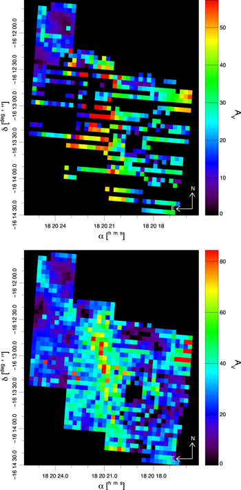
Figure 20. Visual extinction ( ) map of M17 determined when assuming a mixed model and the
  extinction curve from Weingartner & Draine (2001; top) and from Chiar & Tielens (2006; bottom). See Section 5.5 for details.
Download figure:
Standard image High-resolution imageFigure 21 explores the impact of the choice of extinction curve on the measured 6.2/11.2 μm PAH band strength ratio, together with the associated PAHdb-derived  ratio and the large PAH fraction. The figure shows that this impact can be as much as 40% when choosing either the
  extinction curve from Weingartner & Draine (2001) or that from Chiar & Tielens (2006). Despite this, the overall results for M17 and their interpretation when using the extinction curve from Chiar & Tielens (2006) do not change. However, care needs to be taken when choosing an extinction curve, and, in the case of M17 here, that from Chiar & Tielens (2006) could be considered "better," as it avoids the "banded" behavior in the visual extinction map; cf. Figure 20.
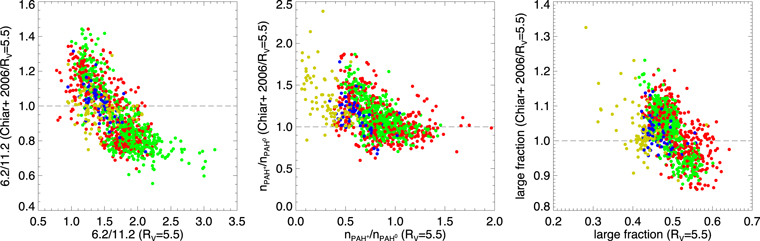
Figure 21. Impact of the choice of extinction curve on the measured 6.2/11.2 μm PAH band strength ratio (left), together with the associated PAHdb-derived  ratio (middle) and large fraction (right) for M17. Each data point is color-coded according to its associated zone in Figure 3. See Section 5.5 for details.
Download figure:
Standard image High-resolution image
5.6. Final Thoughts
Besides the choice of extinction curve (Section 5.5), the results presented here also rely strongly on the contents of PAHdb's spectral libraries and, as described in BBA16, on the spectral resolution of the astronomical data, the details of the employed PAH emission model, and the fitting algorithm used.
As far as the contents of PAHdb's spectral libraries are concerned, it is very difficult to fully and quantitatively assess the influence of their (in)completeness on the accuracy of the PAH subclass breakdown. However, in BBA15, it was shown that, at this stage, the breakdown and calibration of the PAH charge using a two-level system is robust. In addition, Andrews et al. (2015) showed that the spectral breakdown into any PAH subclass can be done reliably. Nonetheless, while the overall quality of the PAHdb fits is considered good, they have difficulties matching some of the emission. Notable are the 6.2 μm PAH feature and the PAH emission originating between 10 and 15 μm. In addition, the contribution from PAH anions to the spectrum is unreasonable (see also BBA16). The following three paragraphs discuss each of these in turn.
Hudgins et al. (2005) suggested that the 6.2 μm band may be attributed to PANHs, PAHs containing nitrogen, and subsequent analysis of the emission from the northwest PDR in NGC 7023 required PANH cations to fit the bulk of the emission in the 6.2 and 11.0 μm bands (BBA13). However, the majority of large PANHs in the PAHdb spectroscopic libraries is limited to a collection of isomers in which the loci of the nitrogen atom are permuted rather than a collection of structurally different PANH molecules. The computation of the spectra of a large variety of (large) PANHs and adding them to PAHdb is required to further test this suggestion.
The emission between 10 and 15 μm is attributed to the CHoop vibrational motion of peripheral hydrogen atoms. Each of the distinct bands in the 10–15 μm is associated with a particular hydrogen adjacency class—the number of neighboring hydrogen atoms protruding from a single aromatic ring, namely, the 11.2, 12.0, 12.7, and 13.5 μm PAH bands with the solo, duo, trio, and quartet adjacency classes, respectively (e.g., Hony et al. 2001; Bauschlicher et al. 2009). Currently, PAHdb's spectral libraries are limited in the number of large PAHs with varying adjacency classes. Most of the larger PAHs ( ) have condensed structures and are part of a series where one characteristic is permuted, e.g., the location of a seven-membered ring defect (Bauschlicher 2015). The computation of a large variety of spectra of large PAHs covering all hydrogen adjacency classes and adding them to PAHdb is required to overcome this limitation.
Although the presence of PAH anions in space has been suggested (e.g., Bregman & Temi 2005; Bauschlicher et al. 2009), their contribution in the PAHdb breakdown spectra here is highly uncertain. Bands with red wings and shoulders are intrinsic to emission from highly vibrationally excited molecules because of the anharmonicity of the vibrational potential, and the current emission models available do not treat anharmonic effects. This is the reason only two ionization states (neutral and positive), with singly and doubly charged PAH cations treated as a single class, are considered, with contributions from singly charged PAH anions ignored. Extending PAHdb to include computed PAH spectra that treat the effects of anharmonicity and/or enhance the employed PAH emission model to better treat anharmonicity should help overcome this issue. For recent efforts to understand PAH anharmonic effects on a fundamental spectroscopic level, see, e.g., Maltseva et al. (2015), Mackie et al. (2016), and Candian & Mackie (2017) and references therein. Inclusion of anharmonic effects in the PAHdb emission models is planned once they are better understood.
6. Summary and Conclusions
Spitzer SL spectral map data on NGC 7023 (RN), M17 (H ii region), and NGC 40 (PN) were analyzed using the data and tools available through PAHdb. After isolating the PAH spectrum from other emission components and correcting for extinction, the PAH spectrum was fitted with modeled PAH emission spectra from PAHdb. Subsequently, the astronomical PAH spectrum was broken down in terms of PAH charge, i.e., anion, neutral, and cation. From the same spectra, the 6.2/11.2 and 8.6/11.2 μm PAH band strength ratio proxies for PAH charge were determined using a traditional approach of isolating the PAH bands. In addition, the strength of  lines was measured and used in population diagrams to derive the
  ortho-to-para ratio, density, and gas temperature.
The 6.2/11.2 μm PAH band strength ratio proxy for the PAH charge has been successfully calibrated against its PAHdb equivalent: the  ratio. Subsequently, the
  ratio was converted into the PAH ionization parameter, which relates it to the strength of the radiation field, gas temperature, and electron density.
The bifurcated 8.6 versus 11.2 μm PAH band strength plot for the northwest PDR in the RN NGC 7023 was shown to be a robust diagnostic template for the  ratio. The diagnostic template clearly highlights not only the different astronomical environments probed in the diffuse and dense media of the PDR region but also how conditions differ between object type.
Template spectra for the three PAH charge subclass components, i.e., anion, neutral, and cation, were determined and shown to favorably intercompare. The SSIM index was utilized as a measure for "likeness" between the morphology of the  ratio maps determined from fitting the spectra with a linear combination of the PAH charge template spectra determined for NGC 7023 and a full PAHdb analysis. The SSIM index showed an overall acceptable comparison for NGC 7023. However, not all performed equally well, with NGC 40 faring the worst.
Motivated by the appearance of banding in some of the M17 extinction maps, the choice of extinction curve was investigated. The interplay between the visual extinction (AV) and other fitted emission components caused a degenerative instability. For M17, there was as much as a 40% difference between the determined PAH band strength ratios and derived PAH subclass components when changing extinction curve. Since these ratios mostly vary in tandem, the overall conclusions of this work stand.
The overall conclusion of this work is that the distinctly different astronomical environments of an RN, H ii region, and PN are reflected in their PAH emission spectra. Moreover, how the PAH population responds—and, in turn, the PAH emission spectra—to changing local physical conditions is entirely dependent on that environment. Extending the analysis presented here to different object types will deepen our understanding of the evolution of the interstellar PAH family and the roles PAHs play in the astrophysics of each environment.
This work is based on observations made with the Spitzer Space Telescope, which is operated by the Jet Propulsion Laboratory, California Institute of Technology, under NASA contract 1407. Support from NASA's Laboratory Astrophysics "Carbon in the Galaxy" consortium grant (NNH10ZDA001N); NASA's Astrobiology, Astronomy + Physics Research and Analysis (APRA; NNX07AH02G); the Astrophysics Data Analysis Program (ADAP; NNH12ZDA001N, NNH14ZDA001N, and NNH16ZDA001N); and Spitzer Space Telescope Support Programs (50082) are greatly acknowledged. CB is grateful for an appointment at the NASA Ames Research Center through the San José State University Research Foundation (NNX14AG80A and NNX17AJ88A). LJA and JB are both thankful for an appointment at the NASA Ames Research Center through the Bay Area Environmental Research Institute (80NSSC17M0014). The anonymous referee is gratefully acknowledged for insight and useful comments.
Facility: Spitzer (IRS) - .
Software: CUBISM (Smith et al. 2007a), MPFIT (Markwardt 2009), IDL Astronomy User's Library (Landsman 1993), AmesPAHdbIDLSuite (Boersma et al. 2014a).
Footnotes
- 1
- 2
The AmesPAHdbIDLSuite can be obtained from http://www.astrochemistry.org/pahdb/downloads or the development version from https://github.com/pahdb/amespahdbidlsuite.
- 3
IDL is a registered trademark of Harris Geospatial.
- 4
Note that there is considerable uncertainty associated with the used parameters that depend on the adopted electron recombination rates. The difference between the classical and measured rates on very small PAHs can be as high as an order of magnitude (cf. Tielens 2005).
- 5
These template spectra can be obtained from http://www.astrochemistry.org/pahdb/templates/ as separate downloads.
- 6
At the time of writing, the SSIM Matlab code could be obtained from http://www.cns.nyu.edu/~lcv/ssim/.
- 7
The IDL implementation of the algorithm for calculating the SSIM index between two images can be downloaded from https://github.com/pahdb/ssim.