


Abstract
We report results from an exploratory study implementing a new probe of Galactic evolution using archival Hubble Space Telescope imaging observations. Precise proper motions are combined with photometric relative metallicity and temperature indices, to produce the proper-motion rotation curves of the Galactic bulge separately for metal-poor and metal-rich main-sequence samples. This provides a "pencil-beam" complement to large-scale wide-field surveys, which to date have focused on the more traditional bright giant branch tracers. We find strong evidence that the Galactic bulge rotation curves drawn from "metal-rich" and "metal-poor" samples are indeed discrepant. The "metal-rich" sample shows greater rotation amplitude and a steeper gradient against line-of-sight distance, as well as possibly a stronger central concentration along the line of sight. This may represent a new detection of differing orbital anisotropy between metal-rich and metal-poor bulge objects. We also investigate selection effects that would be implied for the longitudinal proper-motion cut often used to isolate a "pure-bulge" sample. Extensive investigation of synthetic stellar populations suggests that instrumental and observational artifacts are unlikely to account for the observed rotation curve differences. Thus, proper-motion-based rotation curves can be used to probe chemodynamical correlations for main-sequence tracer stars, which are orders of magnitude more numerous in the Galactic bulge than the bright giant branch tracers. We discuss briefly the prospect of using this new tool to constrain detailed models of Galactic formation and evolution.
Export citation and abstract BibTeX RIS
1. Introduction
The diversity of observed properties of the Galactic bulge has challenged attempts to provide a coherent explanation for its formation and subsequent development. For example, while color–magnitude diagrams (CMDs) suggest that the majority of bulge stars are likely older than ∼8 Gyr (e.g., Kuijken & Rich 2002; Zoccali et al. 2003; Clarkson et al. 2008; Calamida et al. 2014; although see, e.g., Nataf & Gould 2012; Haywood et al. 2016; Bensby et al. 2017, for alternative interpretations), minority populations of younger objects have been detected (e.g., Sevenster et al. 1997; van Loon et al. 2003). That measurements of even bulk parameters like bar orientation and axis ratio have not converged with time (e.g., Vanhollebeke et al. 2009) is consistent with a dependence of these properties on the ages of the tracers used. For example, Catchpole et al. (2016) find distinct bar/bulge spatial structures coexisting in the same volume, traced by Mira populations of different estimated ages. As shown by Ness et al. (2013a), the various apparent observational contradictions may be resolved by a scenario in which most bulge stars did indeed form early but later were rearranged into their present-day spatial and kinematic distributions by disk-driven evolution. Recent reviews of Galactic bulge observations and formation scenarios include Rich (2015), Babusiaux (2016), Zoccali & Valenti (2016), and Nataf (2017).
Observations have long suggested a codependence between chemical abundance and kinematics in the bulge, particularly as traced by velocity dispersion, providing an observational test of formation and evolution scenarios (e.g., Rich 1990; Minniti 1996). Metal-rich samples show a steeper increase in radial velocity dispersion with Galactic latitude than do the metal-poor objects (whose dispersion-latitude profile at latitude  is only gently sloped and may be flat). While differences exist in the literature as to the [Fe/H] cuts used to define the two samples, for latitudes
  the metal-poor and metal-rich samples have consistent radial velicity dispersions (Figure 4 of Babusiaux (2016) presents a recent compilation for fields along the bulge minor axis). For the very innermost fields in the bulge (
 and
and  ), a radial velocity dispersion "inversion" may even be present (an expression of a steeper dispersion gradient with longitude for metal-rich objects), with the metal-rich stars showing greater velocity dispersion than the metal-poor objects in bins closest to the Galactic center (e.g., Babusiaux et al. 2014; Zoccali et al. 2017).
Turning to proper motions, Spaenhauer et al. (1992) traced the proper-motion dispersion for a sample of 57 bulge giants toward Baade's window, allowing the first test of bulge chemical and kinematic codependence using proper motions. No statistically significant discrepancy in proper-motion dispersion was found between metal-poor (defined as [Fe/H] < 0.0) and metal-rich ([Fe/H] > 0.0) objects (with Galactic latitudinal proper-motion dispersion difference Δσμ,l ≈ 0.5 ± 0.6 mas yr−1 between the samples), although the sample size was not large. Zhao et al. (1994) combined the Spaenhauer et al. (1992) ground-based proper motions with published radial velocities and metallicities to demonstrate a break in vertex deviation near [Fe/H] ∼ −0.5. Soto et al. (2007, 2012) demonstrated consistent variation of vertex deviation using Hubble Space Telescope (HST) proper motions for bright giants (for which spectroscopic abundances and radial velocities completed the set of observational parameters; Babusiaux (2016) shows a more recent compilation of vertex deviation as a function of metallicity).
The implications of observational chemical-dynamical correlations for formation models of the inner Milky Way are the subject of vigorous ongoing observational and theoretical research. For example, Debattista et al. (2017) showed that samples drawn from a continuous metallicity distribution in a pure-disk galaxy model can be "kinematically fractionated" by bar formation into metal-rich and metal-poor populations with quite different morphology and dynamics, depending on their initial (galactocentric) radial velocity dispersions. (In this scenario, radial velocity dispersion and metallicity each correlate with the time at which the population formed; thus, they correlate with each other.) This is consistent with the tendency of the "X" shape to be preferentially populated by metal-rich stars (e.g., Vásquez et al. 2013, although the magnitude of this preference is somewhat uncertain; see, e.g., Nataf et al. 2014). Bias in the "X" shape toward metal-rich stars has now also been observed in NGC 4710, a nearby disk-dominated galaxy viewed almost edge-on (Gonzalez et al. 2016, 2017).
Shen et al. (2010) argue that the radial velocities and morphology of bulge stellar populations show no need for a substantial spheroidal "classical" bulge component (at the level of ≲8% of the disk mass), arguing that the Milky Way can be characterized as a pure-disk galaxy. Nonetheless, a small spheroidal component probably has been detected, although its likely contribution to the total bulge mass is likely well under 10% (Kunder et al. 2016). Interpretation of this component in the context of Galactic formation is not clear; it might, for example, represent part of the halo population that has also probably been detected in the inner Milky Way (Koch et al. 2016).
1.1. Does Bulge Rotation Depend on Metallicity?
In addition to velocity dispersion trends, the trend in bulge mean radial velocity (against Galactic longitude or galactocentric radius) might also be expected to vary with metallicity, but here the magnitude (or even existence) of such a dependence is less clear. Earlier spectroscopic surveys suggest a clear difference between metal-poor and metal-rich samples. For example, Harding & Morrison (1993) and Minniti (1996) demonstrated that "metal-rich" stars show a gradient in circular speed with galactocentric radius, consistent with the "solid-body"-type rotation traced by planetary nebulae (Kinman et al. 1988), Mira variables (Menzies 1990), and SiO masers (Nakada et al. 1993). In contrast, metal-poor objects (using [Fe/H] ≲ −1.0, and thus likely including a large contribution from the inner halo) showed no strong evidence for a rotational trend. More recently, Kunder et al. (2016) found that their metal-poor RR Lyrae sample with mostly subsolar metallicities (−2.4 < [Fe/H] ≲ +0.3, peaking at [Fe/H] ∼ −1.0) shows no strong signature of rotation from radial velocities in any Galactic latitude range. This is in contrast to the majority-bulge population, which shows bulk rotation with amplitude vGC ± ≈80 km s−1 progressing from the first to fourth Galactic quadrant (e.g., Howard et al. 2009; Kunder et al. 2016). This rotation-free component is estimated to be a rather small part of the overall bulge stellar population (Kunder et al. 2016).
Restricting attention to [Fe/H] ≳ −1.0 (to sample mainly bulge and disk stars), the body of more recent spectroscopic studies does not show strong evidence for metallicity dependence of radial velocity rotation curves (usually plotted against Galactic longitude). For example, the ARGOS survey (Ness et al. 2013b) and the Gaia-ESO survey (Williams et al. 2016) each show no strong difference between metal-rich and metal-poor bulge objects (the studies use slightly different cuts for metal-rich and metal-poor objects). However, the Giraffe Inner-Bulge Survey (GIBS, which is unusual among the spectroscopic studies in reaching as close as b = −2° to the Galactic midplane) shows a possible difference in rotation curve slope between objects at ![$[\mathrm{Fe}/{\rm{H}}]\lt -0.3$](https://content.cld.iop.org/journals/0004-637X/858/1/46/revision1/apjaaba7fieqn5.gif) and [Fe/H] > +0.2; however, at about 1.5σ significance, the difference is not yet compelling (Zoccali et al. 2017). Thus, the radial velocity surveys focusing on the majority-bulge population (with [Fe/H] ≳ −1.0) show no strong metallicity dependence in the trends of mean radial velocity against Galactic longitude.
and [Fe/H] > +0.2; however, at about 1.5σ significance, the difference is not yet compelling (Zoccali et al. 2017). Thus, the radial velocity surveys focusing on the majority-bulge population (with [Fe/H] ≳ −1.0) show no strong metallicity dependence in the trends of mean radial velocity against Galactic longitude.
Proper motions offer an independent method to kinematically chart the bulge rotation curves and, if information on chemical composition is available, explore whether multiple abundance samples really do show distinct mean motions, as well as the well-established velocity dispersion differences.
To date, proper-motion investigations in the context of multiple populations (or a continuum) have mostly been performed using bright giants. For example, in addition to the vertex deviation investigations reported in the previous section, proper motions of bulge giants using OGLE (Poleski et al. 2013) and with the Wide Field Imager on the La Silla 2.2 m telescope (Vásquez et al. 2013) have been used to uncover azimuthal streaming in the bulge X-shaped structure. However, Qin et al. (2015) caution via N-body models that the underlying bar pattern speed cannot directly be constrained just from the near-side/far-side longitudinal proper-motion difference.
The above radial velocity and proper-motion studies all use bright giants as tracers, often red clump giants (RCGs), which are much less spatially crowded from the ground than are main-sequence (MS) objects. This causes them to be limited by the small intrinsic population size per field of view. For example, ARGOS typically observed about 600 stars at [Fe/H] > −1.0 per 2◦-diameter field of view (Ness et al. 2013b). Thus, mean velocities interpreted for rotation trends represent averages both over quite large angular regions on the sky and, more importantly, over the entire distance range along the line of sight.
To make further progress, an independent measure of bulge rotation is needed, using a tracer sample sufficiently populous that the sample can be dissected by line-of-sight distance to mitigate the statistical limitations of giant branch tracers. MS tracers are orders of magnitude more common on the sky, affording the opportunity to dissect a single sight line along the line of sight, thus offering a "pencil-beam" complement to the wide-field surveys that use the bright end of the CMD.9
It is the charting of the chemically dissected bulge rotation curve from MS proper motions that we report here. Because this is a relatively new technique, we briefly review the short literature in MS proper-motion bulge rotation curve determination before proceeding further.
1.2. Proper Motions of Main-sequence Bulge Populations
Proper-motion-based rotation curves10 from MS bulge stars are relatively rare in the literature.11 Kuijken & Rich (2002) were the first to demonstrate the approach for MS populations, for both the Baade and Sagittarius windows, presenting the HST/WFPC2-derived rotation and dispersion curves against photometric parallax (with photometric parallax determined as a linear combination of color and magnitude in order to remove the color–magnitude slope of the MS tracer population of interest). This demonstrated a clear sense of rotation, with the near side of the bulge showing positive mean longitudinal proper motion relative to the far side (a determination made before the much brighter RCGs were used to show bulge rotation from proper motions; Sumi et al. 2004). The proper-motion dispersion showed a slight increase in the most populous middle bins of photometric parallax (most strongly pronounced in the latitudinal proper-motion dispersion σb) for their Sagittarius window field. Kuijken (2004) presented an extension of this work to multiple fields across the bulge, including the use of three minor-axis fields to estimate the vertical gravitational acceleration along the Galactic minor axis.
Kozłowski et al. (2006) were able to demonstrate similar behavior to the Kuijken & Rich (2002) rotation curves in their analysis of proper motions in Baade's window. This was the only field for which a sufficiently large sample of sufficiently precisely measured MS stars could be measured from their large 35-field study (which used WFPC2 for early-epoch observations and ACS/HRC for late-epoch observations). While their dispersion curve is consistent with a flat distribution, the rotation trend in Galactic longitude was clearly observed. Kozłowski et al. (2006) may also have been the first to detect the weak trend in latitudinal proper motion μb due to solar reflex motion (see Vieira et al. 2007, for discussion of this effect, including its detection using sets of ground-based observations of bulge giants over a 21 yr time baseline). In any case, Kozłowski et al. (2006) were the first to detect the proper-motion correlation Cl,b at statistical significance from any population (using the RCGs that formed their main target population), using it to constrain the tilt angle of the bulge velocity ellipsoid. As they point out, detection of Cl,b (or equivalently the orientation angle ϕlb of the proper-motion ellipsoid) allows constraints to be placed on the orbit families for bulge populations, although the conversion from observation to physical constraint is not simple (e.g., Zhao et al. 1994; Häfner et al. 2000; Rattenbury et al. 2007).
Clarkson et al. (2008, hereafter Cl08) extended the rotation curve approach, using a much deeper data set with ACS/WFC toward the Sagittarius window, estimating photometric parallax directly with reference to a fiducial isochrone describing the average population in the CMD. Consistent with Kuijken & Rich (2002) and Kozłowski et al. (2006), this showed a clear sense of rotation in Galactic longitude, a clear detection of the latitudinal proper-motion trend from near side to far side, and a pronounced peak in the velocity dispersion of both coordinates (σl and σb) coincident with the most densely populated section of the photometric distance range of the sample. Cl08 converted proper motions to velocities, charting the run of the mean velocity (i.e., the rotation curves), the semiminor and semimajor axis lengths (i.e., the velocity dispersions), and the variation of the orientation ϕlb of the projected velocty ellipse with line-of-sight distance, and verified through simulation and comparison with the behavior of RCGs that indeed distance effects are observable in MS photometric parallax (though unlike RCG tracers, unresolved binaries blur somewhat the inferred distances for a given MS population).
More recently, in a careful study of three off-axis bulge fields using WFPC2 for early-epoch observations and ACS/WFC for the late epoch, Soto et al. (2014) were able to extract the rotation curve (and associated proper-motion dispersion curves) for a field farther from the midplane, at (l, b) = (+3 58, −717).12
Soto et al. (2014) also computed the run of velocity ellipse orientation ϕlb with photometric distance, finding trends consistent with Cl08. The kinematics of MS objects at some distance from the plane were thus established to be broadly similar to those at the more central Baade and Sagittarius window fields.
58, −717).12
Soto et al. (2014) also computed the run of velocity ellipse orientation ϕlb with photometric distance, finding trends consistent with Cl08. The kinematics of MS objects at some distance from the plane were thus established to be broadly similar to those at the more central Baade and Sagittarius window fields.
Ground-based surveys are now starting to measure proper motions for MS bulge objects. For example, proper motions from the VVV survey have already been used to draw proper-motion rotation curves for both giant branch and upper MS populations (although the upper MS population shows much higher proper-motion scatter and substantially different selection effects compared to the giants; Smith et al. 2018).
The lack of metallicity information for MS populations has limited both the measurement accuracy and scientific applicability of MS proper-motion rotation curves. The [Fe/H] spread for bulge populations contributes a scatter of up to ∼1 mag on the MS (e.g., Haywood et al. 2016), competing with the photometric parallax signal due to the intrinsic distance distribution along the line of sight. While comparison with the behavior of RCGs suggests that indeed the rotation curve can be recovered, a lack of [Fe/H] information for the MS tracers contributes to substantial mixing in photometric parallax that can dilute the signature of underlying rotation (Clarkson et al. 2008). Conversely, charting bulge proper-motion rotation curves from samples partitioned by relative metallicity allows an independent probe of the chemical and dynamical correlations resulting from the complex formation and evolutionary processes at work in the inner Milky Way.
1.3. Main-sequence Proper Motions for Multiple Populations
Until recently, no observational data set existed that would allow the proper-motion-based rotation curves to be charted for multiple spatially overlapping MS metallicity samples in the bulge, as the relevant tracer samples (a few magnitudes beneath the MS turnoff, and well clear of the subgiant and giant branches in the CMD) are far too faint and spatially crowded for objects to be chemically distinguished using current spectroscopic technology.
The situation changed with the WFC3 Bulge Treasury Survey (hereafter BTS; Brown et al. 2009), which used three-filter flux ratios to construct a "temperature" index ![$[t]$](https://content.cld.iop.org/journals/0004-637X/858/1/46/revision1/apjaaba7fieqn6.gif) (a function of F555W, F110W, and F160W magnitudes, similar to V, J, H) and a "metallicity" index
(a function of F555W, F110W, and F160W magnitudes, similar to V, J, H) and a "metallicity" index ![$[m]$](https://content.cld.iop.org/journals/0004-637X/858/1/46/revision1/apjaaba7fieqn7.gif) (using F390W, F555W, and F814W magnitudes, similar to Washington-C, V, I), with scale factors chosen so that
(using F390W, F555W, and F814W magnitudes, similar to Washington-C, V, I), with scale factors chosen so that ![$[t]$](https://content.cld.iop.org/journals/0004-637X/858/1/46/revision1/apjaaba7fieqn8.gif) and
and ![$[m]$](https://content.cld.iop.org/journals/0004-637X/858/1/46/revision1/apjaaba7fieqn9.gif) are relatively insensitive to reddening. This allows stars to be chemically tagged in a relative sense by their location in
are relatively insensitive to reddening. This allows stars to be chemically tagged in a relative sense by their location in ![$[m]$](https://content.cld.iop.org/journals/0004-637X/858/1/46/revision1/apjaaba7fieqn10.gif) ,
, ![$[t]$](https://content.cld.iop.org/journals/0004-637X/858/1/46/revision1/apjaaba7fieqn11.gif) space, down to much fainter limits and in regions of higher spatial density than currently allowed by spectroscopy. Brown et al. (2010) showed that indeed the wide bulge metallicity range can be traced photometrically by this method, setting
space, down to much fainter limits and in regions of higher spatial density than currently allowed by spectroscopy. Brown et al. (2010) showed that indeed the wide bulge metallicity range can be traced photometrically by this method, setting ![$[t]$](https://content.cld.iop.org/journals/0004-637X/858/1/46/revision1/apjaaba7fieqn12.gif) and
and ![$[m]$](https://content.cld.iop.org/journals/0004-637X/858/1/46/revision1/apjaaba7fieqn13.gif) indices for tens of thousands of MS objects in each of the four observed bulge fields. Inverting the photometric indices then produced relative [Fe/H] distributions broadly similar to the spectroscopic indications from much brighter objects (e.g., Hill et al. 2011; Johnson et al. 2013). Computing these indices appropriately for objects near the bulge MS turnoff, Brown et al. (2010) found that the candidate exoplanet hosts of the SWEEPS field (Sahu et al. 2006) tend to pile up at the metal-rich end of the
indices for tens of thousands of MS objects in each of the four observed bulge fields. Inverting the photometric indices then produced relative [Fe/H] distributions broadly similar to the spectroscopic indications from much brighter objects (e.g., Hill et al. 2011; Johnson et al. 2013). Computing these indices appropriately for objects near the bulge MS turnoff, Brown et al. (2010) found that the candidate exoplanet hosts of the SWEEPS field (Sahu et al. 2006) tend to pile up at the metal-rich end of the ![$[m]$](https://content.cld.iop.org/journals/0004-637X/858/1/46/revision1/apjaaba7fieqn14.gif) distribution as expected, suggesting that
distribution as expected, suggesting that ![$[m]$](https://content.cld.iop.org/journals/0004-637X/858/1/46/revision1/apjaaba7fieqn15.gif) is indeed tracking metallicity. Exploitation of this unique data set to directly constrain the star formation history of the bulge is ongoing (see Gennaro et al. 2015, for an example of the techniques involved).
is indeed tracking metallicity. Exploitation of this unique data set to directly constrain the star formation history of the bulge is ongoing (see Gennaro et al. 2015, for an example of the techniques involved).
Here we combine the relative metallicity estimates from WFC3 BTS photometry with ultradeep proper motions using ACS/WFC, to construct the proper-motion-based rotation curves of candidate "metal-poor" and "metal-rich" MS samples, and examine whether and how the kinematics of the two samples differ from each other. Our work represents the first extension of chemodynamical studies of the bulge down to the MS.
This paper is organized as follows. The observational data sets are introduced in Section 2, with the techniques used to classify samples as "metal-poor" or "metal-rich" and to draw rotation curves described in Section 3. The rotation curves themselves are presented in Section 4. Section 5 discusses the implications of our results for the distribution of populations within both the bulge and proper-motion sample selection and discusses the impact of various systematic effects, with conclusions outlined in Section 6. Appendices A–I provide supporting information, including the full set of results in tabular form.
2. Observations
By the standards of modern proper-motion measurements with HST (e.g., Sahu et al. 2017), the relative streaming motions of the near- and far-side bulge populations are not small, the mean motion of the bulge near side being typically Δμl ∼ 2 mas yr−1 relative to the far side, while the foreground disk is separated from the bulge by relative proper motion  mas yr−1, although the intrinsic proper-motion dispersion is of roughly similar magnitude (Calamida et al. 2014). Thus, extraction of proper-motion-based rotation curves should in general be reasonably straighforward for many bulge fields for which multiple epochs are available.
For this exploratory study, however, we choose the deepest and most precisely measured sample of HST proper motions available toward the bulge, to minimize complications due to completeness effects and varying measurement uncertainty. This is the SWEEPS data set, which, with many epochs over a 9 yr time baseline, represents the current state of the art in space-based proper-motion measurement toward the bulge with HST (e.g., Calamida et al. 2015, Kains et al. 2017). We attached SWEEPS proper motions (Section 2.1) to the BTS photometry (Section 2.2), to afford the maximum sensitivity to proper motions for populations that we can label chemically in a relative sense. Table 1 summarizes the observations.
Table 1. Provenance of the Observational Data Sets Used in This Work
| Data Set | Program (PI) | Observation Dates | Instrument | Filters or Wavelength range | Nall | Sections |
|---|---|---|---|---|---|---|
| SWEEPS | HST GO-9750 (Sahu) | 2004 Feb (MJD 53060) | HST-ACS/WFC | F606W, F814W | 339,193 | Section 2.1 |
| HST GO-12586 (Sahu) | 2011 Oct–2013 Oct | |||||
| HST GO-13057 (Sahu) | (MJD 56333) | |||||
| BTS | HST GO-11664 (Brown) | 2010 May | HST-WFC3/UVIS | F390W, F555W, F814W | 52,596 | Section 2.2 |
| HST-WFC/IR | F110W, F160W | |||||
| VLT | ESO 073.C-0410(A) | 2004 Jun | VLT-UT2/UVES | 4812–5750 Å | 123 | Appendix C.1 |
| (Minniti) | 5887–6759 Å | |||||
Note. Nall represents the number of objects in each catalog (with measurements in all filters for SWEEPS and BTS). The median modified Julian dates are indicated for the 2004 and the 2011–2012–2013 SWEEPS epochs. The SWEEPS field lies at (α, δ)J2000.0 ≈ (17:59:00.7, −29:11:59.1), or (l, b)J2000.0 ≈ (+126, −265).
Download table as: ASCIITypeset image
Figure 1 presents a finding chart. The observations cover a single ACS/WFC field of view (∼3 4 × 34) in the Sagittarius window, a low-reddening region (
 ≈ 0.5–0.7, depending on the reddening prescription; e.g., Ca15) that is close in projection to the Galactic center (l, b = 126, −265).
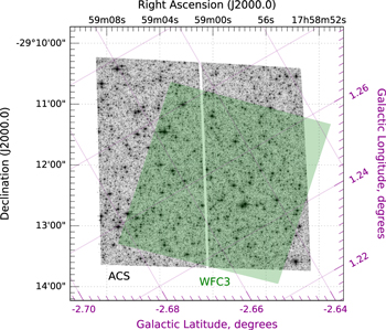
Figure 1. Finding chart for the SWEEPS ACS/WFC and BTS WFC3 data sets used in this work. The tilted solid dark magenta grid shows Galactic coordinates, spaced at 002 intervals. The dotted gray grid shows equatorial coordinates, spaced at 1' intervals. The green polygon shows the BTS WFC3 coverage; our sample is drawn from the region of overlap between the two surveys. North is up, east left, and the ACS/WFC field of view is approximately 34 × 34, centered approximately at (α, δ)J2000.0 = (17:59:00.7, −29:11:59.1), or  . See Section 2.
Download figure:
Standard image High-resolution image2.1. SWEEPS Photometry and Proper Motions
The SWEEPS data set used here consists of an extremely deep imaging campaign with a 9 yr time baseline using ACS/WFC in F606W and F814W (programs GO-9750, GO-12586, and GO-13057; PI K. C. Sahu). The observations and analysis techniques used to produce the proper motions and photometry used herein are described in some detail in previous papers (Sahu et al. 2006, hereafter Sa06; Cl08; Calamida et al. 2014, hereafter Ca14; Calamida et al. 2015, hereafter Ca15; Kains et al. 2017). Here we briefly describe the relevant characteristics for the present study.
Stellar positions in individual images were estimated using the distortion solution and effective point-spread function (PSF) methods developed by J. Anderson for HST and implemented for ACS/WFC in the img2xym.F routine (Anderson & King 2006) and associated utilities. This yields highly precise position measurements in a reference frame that is nearly free of distortion. With these techniques, per-measurement random uncertainties are as small as  pixels per coordinate (e.g., Figure 3 of Cl08), and residual distortion is as low as ∼0.01 pixels (Anderson & King 2006; see also Appendix A). Detailed discussion of the methods can be found in Anderson & King (2006) and Anderson et al. (2008a, 2008b).
The 2011–2012–2013 epoch consists of 60 (61) images in F606W (F814W) taken with an approximately 2-week cadence, while the 2004 epoch consists of 254 (265) exposures in F606W(F814W) taken over a 1-week interval in 2004 (Sa06, all exposures in both programs being ≈5.5 minutes each, which well samples the bulge MS and minimizes downtime for buffer dumps).
Because the disk and bulge stars move relative to each other, the 2011–2012–2013 images were reduced separately from those in the 2004 epoch. Proper motions were derived from the best-fit positional differences between the 2004 and 2011–2012–2013 data sets; they thus represent two-epoch proper motions, but with positions in each individual epoch measured to very high accuracy. The positional differences (in ACS/WFC pixels) were rotated into a frame aligned with Galactic coordinates and converted from a displacement in pixels into rate of positional change in mas yr−1 using the ACS/WFC plate scale (50 mas pixel−1 in the distortion-free frame of Anderson & King 2006) and the time baseline between the two epochs (8.96 yr; Table 1). This yields transverse relative motions in mas yr−1 in a frame closely aligned with the Galactic coordinate system.
Without absolute reference-frame tracers in this crowded field (e.g., Yelda et al. 2010; Sohn et al. 2012), we work exclusively with relative proper motions. Zero proper motion  is defined as the median observed rate of positional change for bulge objects across the entire field of view, without any selection for metallicity. The sample defining this proper-motion reference consists of stars that are not saturated in the deep exposures (these objects are at the bulge MS turnoff and fainter).13
Ca15 conducted extensive artificial-star tests to estimate measurement uncertainty in the proper motions, with artificial objects injected with proper motions into individual measurement frames to characterize the random proper-motion uncertainty as a function of apparent magnitude. Including random measurement uncertainty, random intrinsic uncertainty due to tracer star motion, and estimated residual distortion, the proper-motion uncertainty per coordinate is approximately ≲0.12 mas yr−1 over the apparent magnitude range of interest (see Appendix A for details), easily sufficient to measure relative stellar motions in this field.
The result is a set of 339,193 objects with ACS/WFC positions, apparent magnitudes, and proper-motion estimates, all with uncertainties characterized as a function of apparent magnitude. Exploitation of these data is presented in Calamida et al. (2014, 2015) and Kains et al. (2017).
2.2. WFC3 Photometry from the WFC3 Bulge Treasury Project (BTS)
The WFC3 Bulge Treasury Project (BTS; program GO-11664; PI T. M. Brown) visited four fields in the bulge, with WFC3, including the SWEEPS field. The observations are described in detail in Brown et al. (2010); here we briefly summarize the characteristics relevant for the present paper.
In each field, observations were taken in UVIS/F390W (11,180 s), UVIS/F555W (2283 s), UVIS/F814W (2143 s), IR/F110W (1255 s), and IR/F160W (1638 s), with IR images (field of view 123'' × 136'') dithered in order to fully cover the UVIS observations (field of view 162'' × 162''). Good overlap was achieved with the SWEEPS ACS/WFC observations; nearly all the BTS objects in this field also fall within the SWEEPS ACS/WFC field of view (Figure 1).
Version 1 of the BTS catalog,14
which we use here, employed photometry and positions measured with daophotII (Stetson 1987; Brown et al. 2010). The resulting BTS v1 catalog lists 400,424 objects in the Sagittarius window with reported apparent magnitude in any of the BTS filters. Of these, 52,596 have measurements in all five of the BTS filters that are required to construct ![$[t],[m]$](https://content.cld.iop.org/journals/0004-637X/858/1/46/revision1/apjaaba7fieqn25.gif) estimates.
estimates.
3. Analysis
To construct the "metal-rich" and "metal-poor" rotation curves, we used the BTS photometry to draw "metal-rich" and "metal-poor" samples by use of ![$[t],[m]$](https://content.cld.iop.org/journals/0004-637X/858/1/46/revision1/apjaaba7fieqn26.gif) and used the SWEEPS data to estimate the relative photometric parallaxes and proper motions. Within each sample, the relative photometric parallax (
and used the SWEEPS data to estimate the relative photometric parallaxes and proper motions. Within each sample, the relative photometric parallax ( ) for a given star is defined as the apparent magnitude offset from the fiducial ridgeline in the SWEEPS CMD for the sample. The SWEEPS deep (F606W, F814W) CMD was used to estimate
  because this choice of filters is relatively insensitive to metallicity variations when compared to, for example, the (C, V-I) CMD presented in Brown et al. (2010).
This section is organized as follows: Section 3.1 describes the merging of the SWEEPS and BTS catalogs, with the sample selection for proper-motion study discussed in Section 3.2 and the calculation of the photometric indices ![$[t],[m]$](https://content.cld.iop.org/journals/0004-637X/858/1/46/revision1/apjaaba7fieqn29.gif) shown in Section 3.3. These indices require a prescription for extinction, discussed in Section 3.4. The classification into "metal-rich" and "metal-poor" samples is discussed in Section 3.5. The kinematic behavior of the two samples was then measured in two ways; a simple 1D characterization of the longitudinal proper motion
shown in Section 3.3. These indices require a prescription for extinction, discussed in Section 3.4. The classification into "metal-rich" and "metal-poor" samples is discussed in Section 3.5. The kinematic behavior of the two samples was then measured in two ways; a simple 1D characterization of the longitudinal proper motion  is indicated in Section 3.6, while a more sophisticated dissection of the velocity ellipse with relative photometric parallax
  is shown in Section 3.7.
3.1. Merging the ACS/WFC and BTS Catalogs
The BTS and SWEEPS catalogs were first cross-matched by equatorial coordinates. Although the absolute pointing of HST is accurate only to ∼0 1 (Gonzaga et al. 2012), with F814W observations in both data sets,15
matching of similar objects in both catalogs is straightforward (using F555W and F606W measurements in WFC3 and ACS/WFC, respectively, to refine the matches). For the first round of matching, a kd-tree approach was used to cross-match on the sphere, with a 5-pixel radius used for initial matching. In the second round, pixel positions in the two catalogs were cross-matched and fit using a general linear transformation for objects in the
1 (Gonzaga et al. 2012), with F814W observations in both data sets,15
matching of similar objects in both catalogs is straightforward (using F555W and F606W measurements in WFC3 and ACS/WFC, respectively, to refine the matches). For the first round of matching, a kd-tree approach was used to cross-match on the sphere, with a 5-pixel radius used for initial matching. In the second round, pixel positions in the two catalogs were cross-matched and fit using a general linear transformation for objects in the  range. While the population of good matches transitions to a background of mismatched objects at a radius of ∼2 pixels and larger, the vast majority of cross-matches were somewhat better, falling within a 1-pixel matching distance. The matching process resulted in a list of 47,537 objects with proper motions and seven-filter apparent magnitudes, with uncertainty estimates for all quantities.
3.2. Sample Selection for Proper-motion Study
Two aspects of the sample selection are worth highlighting. First, the selection region in the (F606W, F814W) CMD was chosen to be well clear of the MS turnoff, subgiant branch, and giant branch, to encompass as many stars as possible with good proper-motion measurements, and finally to capture a region over which the MS for a given population is reasonably free of curvature in the CMD. This selection region is shown in Table 2 and Figure 2. Second, the photometric metallicity and temperature indices include coefficients that amplify measurement uncertainty (particularly F110W and F160W, which appear in the temperature index ![$[t]$](https://content.cld.iop.org/journals/0004-637X/858/1/46/revision1/apjaaba7fieqn33.gif) ). For this reason, objects were only selected for further study for which all apparent magnitude uncertainties in the photometric catalog are smaller than 0.1 mag.
). For this reason, objects were only selected for further study for which all apparent magnitude uncertainties in the photometric catalog are smaller than 0.1 mag.
The successive selection steps isolating the sample for further study are detailed in Table 3. Of an initial sample of 339,193 SWEEPS objects and 400,424 BTS objects, 9700 (∼2.9%) were retained for further analysis.
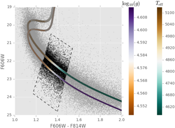
Figure 2. Region selection in the SWEEPS CMD. The dashed polygon shows the selection region for objects selected for proper-motion study (see Section 3.2 and Table 2). To illustrate typical stellar parameter ranges for this sample, also overplotted is a 10 Gyr isochrone at [Fe/H] = −0.09 from the "canonical" α-enhanced set within the BaSTI library (Pietrinferni et al. 2004, using the "F05" opacities of Ferguson et al. 2005). The isochrone is plotted twice, color-coded to show  (left color bar) and
  (right color bar) and offset for clarity, with color minima and maxima set to the range of parameters across the sample of interest. See Sections 3.2 and 3.3.
Download figure:
Standard image High-resolution imageTable 2. Vertices of the Selection Polygon in the SWEEPS CMD That Was Used to Select Objects for Further Proper-motion Study
| (F606W–F814W) | F606W |
|---|---|
| (mag) | (mag) |
| 1.40 | 24.80 |
| 1.54 | 21.30 |
| 1.34 | 20.50 |
| 1.17 | 23.80 |
Note. See Section 3.2 for discussion.
Download table as: ASCIITypeset image
Table 3. Selection Steps Used to Isolate the Proper-motion Sample for Further Study
| Selection | N(remaining) | N(removed) |
|---|---|---|
| SWEEPS sample (Calamida et al. 2014) | 339,193 | ⋯ |
| Cross-matched with BTS | 55,666 | 283,527 |
| BTS measurements in all filters | 47,537 | 8129 |
| Within SWEEPS CMD selection region | 10,225 | 37,312 |
| σmag(ACS/WFC) < 0.1 mag | 10,222 | 3 |
| σmag(WFC3/UVIS) < 0.1 mag | 10,209 | 13 |
| σmag(WFC3/IR) < 0.1 mag | 10,145 | 64 |
Clipping far outliers in ![$[t],[m]$](https://content.cld.iop.org/journals/0004-637X/858/1/46/revision1/apjaaba7fieqn36.gif)
|
9,700 | 445 |
Note. The cuts are cumulative, reading from top to bottom. The third step includes selecting out any rows for which any of the seven phometry and two proper-motion measurements are listed as a "bad" value in either the SWEEPS or BTS catalogs. In practice, this limits the sample to 18.5 ≤ F606W ≤ 27.5. The SWEEPS CMD selection region is shown in Figure 2. For the three instrumental configurations listed, objects must show photometric uncertainty <0.1 mag in all relevant filters: (F606W, F814W) for ACS/WFC, (F390W, F555W, F814W) for WFC3/UVIS, and (F110W, F160W) for WFC3/IR. Objects passing ![$[t],[m]$](https://content.cld.iop.org/journals/0004-637X/858/1/46/revision1/apjaaba7fieqn37.gif) clipping satisfy −3.50 ≤
clipping satisfy −3.50 ≤ ![$[t]$](https://content.cld.iop.org/journals/0004-637X/858/1/46/revision1/apjaaba7fieqn38.gif) ≤ −1.00 and −0.60 ≤
≤ −1.00 and −0.60 ≤ ![$[m]$](https://content.cld.iop.org/journals/0004-637X/858/1/46/revision1/apjaaba7fieqn39.gif) ≤ 0.40. See Section 3.2 for discussion.
≤ 0.40. See Section 3.2 for discussion.
Download table as: ASCIITypeset image
3.3. Production of [t], [m] for the Proper-motion Sample
The photometric indices ![$[t],[m]$](https://content.cld.iop.org/journals/0004-637X/858/1/46/revision1/apjaaba7fieqn40.gif) take the following form (Brown et al. 2009):
take the following form (Brown et al. 2009):

with  and
and  , all of which have a dependence on stellar parameters. The median values of these stellar parameters for the proper-motion sample (
 ≈ 4800 K and log(g) ≈ 4.6) were estimated from an isochrone chosen to overlap the observed sample (see Figure 2; several combinations of metallicity, age, and extinction were tried, indicating that the parameter range for this sample is roughly 4200 K ≲
  ≲ 5200 K and
  ).
).
3.4. Extinction Estimates for Reddening-free Indices
The factors α, β are three-filter extinction ratios (Brown et al. 2009). Synthetic photometry was used to estimate the relationship between reddening and extinction for the objects of interest and to generate reddening vectors in the various filter combinations of interest. For a range of  values, pysynphot was used to generate synthetic stellar spectra, and the run of AX against
  was fit as
  separately for all seven filters used in this study, over the range 0.0 ≤
  ≤ 1.5. The calculation was performed for
  ,
,  appropriate to the SWEEPS CMD region chosen for proper-motion study (Figure 2). The process was repeated for low- and high-metallicity objects to estimate sensitivity of the extinction prescription to metallicity variation within the sample selected for further study, and for (
 ,
,  ) for objects at the median, minimum, and maximum
  within this sample to estimate spread of α, β along the sample.
This procedure requires a prescription for the extinction law toward the bulge. This extinction law appears to be somewhat nonstandard and strongly spatially variable, with some doubt in the literature about whether a single-parameter model can accurately reproduce observed behavior from the visible to the near-infrared (e.g., Nataf et al. 2016, and references therein). As the ![$[t],[m]$](https://content.cld.iop.org/journals/0004-637X/858/1/46/revision1/apjaaba7fieqn55.gif) indices use photometry over a very broad wavelength range (CVIJH, or λ ≈ 350–1700 nm), systematic uncertainties in the extinction prescription will in turn impact any inferences about the underlying metallicity distribution (this is one reason why we use
indices use photometry over a very broad wavelength range (CVIJH, or λ ≈ 350–1700 nm), systematic uncertainties in the extinction prescription will in turn impact any inferences about the underlying metallicity distribution (this is one reason why we use ![$[t],[m]$](https://content.cld.iop.org/journals/0004-637X/858/1/46/revision1/apjaaba7fieqn56.gif) only to classify objects by relative [Fe/H] estimates).
only to classify objects by relative [Fe/H] estimates).
To make progress, we adopted a single-parameter reddening law, but with ratio of selective to total extinction RV = 2.5, as suggested by the investigations of Nataf et al. (2013).16
As this value is not among the standard parameterizations available in pysynphot, the coefficients  for the seven filters were estimated for RV = 2.1 and RV = 3.1 and linearly interpolated to RV = 2.5.
Table 4 shows the kX estimates for each filter, along with the coefficients α, β in the ![$[t],[m]$](https://content.cld.iop.org/journals/0004-637X/858/1/46/revision1/apjaaba7fieqn59.gif) indices. These are quite different from the MS coefficients reported in Brown et al. (2009), as expected since here we are targeting a specific population some way beneath the MS turnoff and have used a different prescription for extinction.
indices. These are quite different from the MS coefficients reported in Brown et al. (2009), as expected since here we are targeting a specific population some way beneath the MS turnoff and have used a different prescription for extinction.
Table 4.
Estimates of  and Derived Parameters
| Config | CCM89, RV = 2.1: log(Z) = −3.3 | CCM89, RV = 2.1: log(Z) = −1.6 | CCM89, RV = 3.1: log(Z) = −3.3 | CCM89, RV = 3.1: log(Z) = −1.6 | CCM89, RV = 2.5: log(Z) = −3.3 | CCM89, RV = 2.5: log(Z) = −1.6 | |
|---|---|---|---|---|---|---|---|
| ACS/WFC1/F606W | 1.847 | 1.849 | 2.786 | 2.788 | 2.222 | 2.224 | |
| ACS/WFC1/F814W | 1.064 | 1.064 | 1.821 | 1.822 | 1.366 | 1.367 | |
| WFC3/UVIS1/F390W | 3.507 | 3.492 | 4.489 | 4.475 | 3.899 | 3.885 | |
| WFC3/UVIS1/F555W | 2.183 | 2.186 | 3.167 | 3.171 | 2.576 | 2.58 | |
| WFC3/UVIS1/F814W | 1.074 | 1.075 | 1.833 | 1.834 | 1.377 | 1.378 | |
| WFC3/IR/F110W | 0.560 | 0.558 | 1.025 | 1.021 | 0.746 | 0.743 | |
| WFC3/IR/F160W | 0.345 | 0.345 | 0.635 | 0.634 | 0.461 | 0.460 | |
| (F606W–F814W)ACS/WFC1 | 0.784 | 0.785 | 0.965 | 0.966 | 0.856 | 0.857 | |
| α | 7.55 | 7.64 | 5.49 | 5.56 | 6.42 | 6.49 | |
| β | 1.19 | 1.18 | 0.99 | 0.98 | 1.10 | 1.09 | |
Note. Here Teff = 4800.0 and log(g) = 4.59. For convenience, the scale factor for the SWEEPS color index is also shown. The quantities α, β give the extinction ratios relevant for ![$[t],[m]$](https://content.cld.iop.org/journals/0004-637X/858/1/46/revision1/apjaaba7fieqn61.gif) . Specifically,
. Specifically,  and
and  . See Sections 3.3 and 3.4.
Download table as: ASCIITypeset image
For a given choice of RV the variation of all extinction-relevant quantities appears to be small within the sample of interest; α, β each vary by <0.1 between the two abundance sets tested and, for a given abundance, by ≲0.02 across the  range of this sample. We adopt
  for the rest of this work.
3.5. Classifying Samples by Relative Metallicity
The resulting (![$[t],[m]$](https://content.cld.iop.org/journals/0004-637X/858/1/46/revision1/apjaaba7fieqn66.gif) ) distribution of objects is shown in Figure 3. Two concentrations are apparent: one near (
) distribution of objects is shown in Figure 3. Two concentrations are apparent: one near (![$[t]$](https://content.cld.iop.org/journals/0004-637X/858/1/46/revision1/apjaaba7fieqn67.gif) ,
, ![$[m]$](https://content.cld.iop.org/journals/0004-637X/858/1/46/revision1/apjaaba7fieqn68.gif) ) = (−2.0, 0.15), and a second, more elongated concentration with major axis angled at about −45° in Figure 3, centered near (
) = (−2.0, 0.15), and a second, more elongated concentration with major axis angled at about −45° in Figure 3, centered near (![$[t]$](https://content.cld.iop.org/journals/0004-637X/858/1/46/revision1/apjaaba7fieqn69.gif) ,
, ![$[m]$](https://content.cld.iop.org/journals/0004-637X/858/1/46/revision1/apjaaba7fieqn70.gif) ) ≈ (−2.2, −0.1).
) ≈ (−2.2, −0.1).
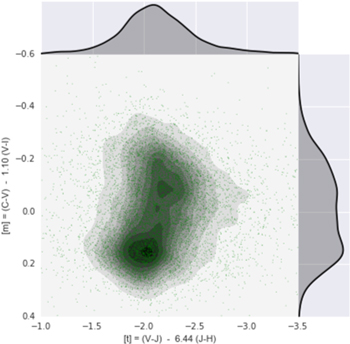
Figure 3.
![$[t],[m]$](https://content.cld.iop.org/journals/0004-637X/858/1/46/revision1/apjaaba7fieqn71.gif) distribution of the population selected for proper-motion study. In the main panel, green points show individual objects, and black contours show the smoothed representation as a 2D kernel density estimate (KDE) with 10 levels plotted. Marginal distributions in
distribution of the population selected for proper-motion study. In the main panel, green points show individual objects, and black contours show the smoothed representation as a 2D kernel density estimate (KDE) with 10 levels plotted. Marginal distributions in ![$[t]$](https://content.cld.iop.org/journals/0004-637X/858/1/46/revision1/apjaaba7fieqn72.gif) and
and ![$[m]$](https://content.cld.iop.org/journals/0004-637X/858/1/46/revision1/apjaaba7fieqn73.gif) are shown in the top and right panels, respectively. Typical estimates for measurement uncertainty in this space are presented in Figure 18. See Section 3.3.
are shown in the top and right panels, respectively. Typical estimates for measurement uncertainty in this space are presented in Figure 18. See Section 3.3.
Download figure:
Standard image High-resolution imageTo classify objects by relative metallicity and thus draw "metal-rich" and "metal-poor" samples for further study, the population highlighted in Figure 2 was characterized as a Gaussian Mixture Model (GMM) in (![$[t]$](https://content.cld.iop.org/journals/0004-637X/858/1/46/revision1/apjaaba7fieqn74.gif) ,
, ![$[m]$](https://content.cld.iop.org/journals/0004-637X/858/1/46/revision1/apjaaba7fieqn75.gif) ) space, and members of the "metal-poor" and "metal-rich" samples were identified by their formal membership probability
) space, and members of the "metal-poor" and "metal-rich" samples were identified by their formal membership probability  (see Appendix B). The number K of mixture components to use was determined by increasing K until the characterization stopped improving (see Appendix B.2 for details). At least two components seem to be required, but a four-component mixture model appears to provide the best representation of the
 ![$[t],[m]$](https://content.cld.iop.org/journals/0004-637X/858/1/46/revision1/apjaaba7fieqn77.gif) distribution.
distribution.
We therefore adopt a four-component GMM to characterize the observed distribution in ![$[t],[m]$](https://content.cld.iop.org/journals/0004-637X/858/1/46/revision1/apjaaba7fieqn78.gif) space for the rest of this work. Table 5 shows the GMM parameters, while Figure 4 presents the model components visually. The two most significant components correspond roughly to visually apparent concentrations in Figure 3, together accounting for 91% of the mixture; these form our "metal-rich" and "metal-poor" samples. The remaining two components, making up about 6% and 3%, do not correspond to any physically obvious population. These two components might represent populations of outlier objects, or structure in the background in (
space for the rest of this work. Table 5 shows the GMM parameters, while Figure 4 presents the model components visually. The two most significant components correspond roughly to visually apparent concentrations in Figure 3, together accounting for 91% of the mixture; these form our "metal-rich" and "metal-poor" samples. The remaining two components, making up about 6% and 3%, do not correspond to any physically obvious population. These two components might represent populations of outlier objects, or structure in the background in (![$[t],[m]$](https://content.cld.iop.org/journals/0004-637X/858/1/46/revision1/apjaaba7fieqn79.gif) ). We retain these low-level components in the GMM for all subsequent work using the BTS catalog, but we do not interpret them as representing any intrinsic population component.
). We retain these low-level components in the GMM for all subsequent work using the BTS catalog, but we do not interpret them as representing any intrinsic population component.
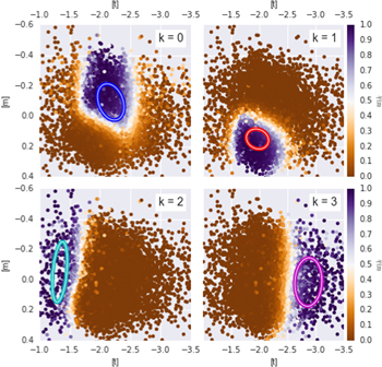
Figure 4.
![$[t],[m]$](https://content.cld.iop.org/journals/0004-637X/858/1/46/revision1/apjaaba7fieqn80.gif) sample color-coded by membership probabilities
sample color-coded by membership probabilities  (Equation (3)) for the k'th model component in the GMM characterization of the observed distribution. The 1σ ellipse for the k'th model component is overplotted in each case as a colored ellipse. Reading clockwise from top left, panels show the "metal-rich," the "metal-poor," and the two background components. See the discussion in Section 3.5.
Download figure:
Standard image High-resolution imageTable 5.
Parameters of the Gaussian Mixture Model in ![$[t],[m]$](https://content.cld.iop.org/journals/0004-637X/858/1/46/revision1/apjaaba7fieqn82.gif) Space for Stars beneath the Main Sequence Selected for Further Study
Space for Stars beneath the Main Sequence Selected for Further Study
| k | Name | αk |
![${[t]}_{0}$](https://content.cld.iop.org/journals/0004-637X/858/1/46/revision1/apjaaba7fieqn83.gif)
|
![${[m]}_{0}$](https://content.cld.iop.org/journals/0004-637X/858/1/46/revision1/apjaaba7fieqn84.gif)
|
![${\sigma }_{[t][t]}^{2}$](https://content.cld.iop.org/journals/0004-637X/858/1/46/revision1/apjaaba7fieqn85.gif)
|
![${\sigma }_{[m][m]}^{2}$](https://content.cld.iop.org/journals/0004-637X/858/1/46/revision1/apjaaba7fieqn86.gif)
|
![${\sigma }_{[t][m]}^{2}$](https://content.cld.iop.org/journals/0004-637X/858/1/46/revision1/apjaaba7fieqn87.gif)
|
|---|---|---|---|---|---|---|---|
( ) ) |
(mag) | (mag2) | (mag2) | (mag2) | |||
| 0 | "Metal-poor" | 0.557 | −2.18 | −0.09 | 0.0479 | 0.0143 | −0.00742 |
| 1 | "Metal-rich" | 0.358 | −1.97 | 0.15 | 0.0384 | 0.0043 | −0.00187 |
| 2 | ⋯ | 0.026 | −1.34 | −0.05 | 0.0153 | 0.0397 | 0.00886 |
| 3 | ⋯ | 0.059 | −2.87 | 0.01 | 0.0573 | 0.0255 | 0.00240 |
Note. Reading left to right, columns indicate the component index k, its label (if any), its (rounded) mixture fraction αk, the two components of its centroid, and the three unique components of the covariance matrix  . See Section 3.5.
Download table as: ASCIITypeset image
This four-component GMM provides the basis for our classification of objects by relative metallicity, with "metal-rich" and "metal-poor" objects corresponding to the two most significant components of the GMM (Table 5).17
A rough estimate for the centroid [Fe/H] values of the two samples may be drawn by charting [Fe/H] contours in the ![$[t],[m]$](https://content.cld.iop.org/journals/0004-637X/858/1/46/revision1/apjaaba7fieqn91.gif) diagram for synthetic stellar populations and interpolating to estimate [Fe/H] at the
diagram for synthetic stellar populations and interpolating to estimate [Fe/H] at the ![$[t],[m]$](https://content.cld.iop.org/journals/0004-637X/858/1/46/revision1/apjaaba7fieqn92.gif) locations of the corresponding GMM component centroids (see Appendix F.1 for more details on the synthetic stellar populations used). The GMM component centroids presented in Table 5 correspond to [Fe/H]0 ≈ +0.18 for the "metal-rich" sample (using scaled-to-solar isochrones) and
locations of the corresponding GMM component centroids (see Appendix F.1 for more details on the synthetic stellar populations used). The GMM component centroids presented in Table 5 correspond to [Fe/H]0 ≈ +0.18 for the "metal-rich" sample (using scaled-to-solar isochrones) and ![${[\mathrm{Fe}/{\rm{H}}]}_{0}\approx -0.24$](https://content.cld.iop.org/journals/0004-637X/858/1/46/revision1/apjaaba7fieqn93.gif) for the "metal-poor" sample (using α-enhanced isochrones for this model component). These centroids are roughly consistent with values suggested from spectroscopic surveys (e.g., Hill et al. 2011; Zoccali et al. 2017).
for the "metal-poor" sample (using α-enhanced isochrones for this model component). These centroids are roughly consistent with values suggested from spectroscopic surveys (e.g., Hill et al. 2011; Zoccali et al. 2017).
For an object to be classified with the "metal-rich" or "metal-poor" sample, it must show formal membership probability  (see Equation (3); note that an object need not be classified with either sample when there are four model components). The shading in Figure 4 visualizes the membership probabilities
  associated with each mixture component. The threshold
  was chosen as a trade-off between sample purity (typical objects should not fall into more than one model component at the chosen threshold) and the need to have a sufficient sample size (at least a few thousand) to permit the dissection of the proper motions by relative photometric parallax with sufficient resolution to chart the rotation curves.
Assigning relative photometric parallax ( ) is the final step required before proper-motion rotation curves can be charted, with reference to fiducial ridgelines for the "metal-rich" and "metal-poor" samples. The fiducial ridgelines themselves were determined by a simple empirical fit to the density of each sample in the SWEEPS CMD. A second-order polynomial adequately represents the median samples and allows very rapid evaluation of relative photometric parallax. Figure 5 shows the adopted fiducial ridgelines for the "metal-rich" and "metal-poor" samples in the SWEEPS CMD, while their parameters are given in Table 6.
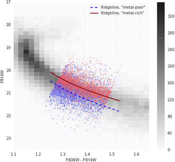
Figure 5. Ridgelines for the "metal-rich" and "metal-poor" samples. The grayscale shows the ACS/WFC (F606W, F814W) Hess diagram for the larger SWEEPS sample. Objects falling within the region of interest for our kinematic study are presented as points, color-coded by "metal-rich" (red) or "metal-poor" (blue). The empirical median-sample ridgelines for the "metal-rich" (dark red solid line) and "metal-poor" (blue dashed line) are overlaid. See Section 3.5 and Table 6.
Download figure:
Standard image High-resolution imageTable 6. Ridgeline Parameters in the SWEEPS Color–Magnitude Diagram, for the "Metal-poor" and "Metal-rich" Samples
| k | Name | a0 | a1 | a2 |
|---|---|---|---|---|
( ) ) |
(mag−1) | |||
| 0 | "Metal-poor" | −16.906 | 48.557 | −14.954 |
| 1 | "Metal-rich" | −5.720 | 33.458 | −10.293 |
Note. These purely empirical ridgelines are used to rapidly evaluate photometric parallax for objects in each sample and take the form  , with x the (F606W – F814W) color. See Section 3.5 for discussion.
Download table as: ASCIITypeset image
3.6. Proper-motion Rotation Curves
Having drawn "metal-rich" and "metal-poor" samples from the BTS photometry, along with fiducial sequences in the SWEEPS CMD for the two samples, the "metal-rich" and "metal-poor" rotation curves can be charted. Figure 6 shows the raw distribution of longitudinal proper motion μl and relative photometric parallax for the "metal-rich" and "metal-poor" samples, with trends presented in Figure 7.
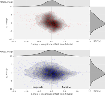
Figure 6. Raw distribution of μl against relative photometric parallax ( ), for the "metal-rich" (red) and "metal-poor" (blue) populations. The near side of the population is to the left in both panels. The points themselves are illustrated by colored scatterplots in the main panels, with density contours indicated in gray scale. The top and right panels show the marginal distributions of
  and μl, respectively. See Section 3.6.
Download figure:
Standard image High-resolution image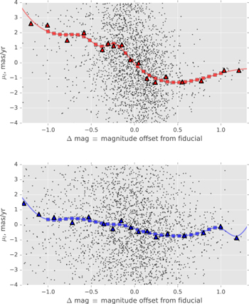
Figure 7. Proper-motion rotation curves. The "metal-rich" sample is denoted in red in the top panel, the "metal-poor" sample in blue in the bottom panel. The population is broken into bins in relative distance modulus and the median value  determined for each bin (triangles). Faint solid lines show a third-order smoothed spline approximation fit to the binned proper motions
  , while squares indicate equally spaced evaluations of the spline approximation over the range of relative moduli (−1.0 ≤ (m − m0) < +1.0). See Section 3.6.
Download figure:
Standard image High-resolution imageAll proper motions in this work were measured relative to the same proper-motion zero-point, defined without reference to any selection by metallicity (Section 2.1). To the extent that the "metal-rich" and "metal-poor" samples trace bulge objects with different spatial distribution and/or kinematic behavior, however, the average proper motions of bulge objects in the two samples might differ.
We therefore estimated the proper motion corresponding to the fiducial sequence for each sample. For this "central" proper motion, we used the median proper motion over those sample members with relative photometric parallax between  and
and  magnitudes nearer to and farther than the fiducial, respectively.18
We adopted
magnitudes nearer to and farther than the fiducial, respectively.18
We adopted  = 0.05, corresponding roughly to Δ
 ≈ 0.18 kpc at the distance of the bulge (Section 4.1). The central proper motion for the "metal-rich" sample is then
  mas yr−1 from 381 surviving objects, while for the "metal-poor" sample we found
  mas yr−1 from 290 surviving objects. The proper motion corresponding to the "metal-rich" fiducial was thus found to be offset from that of the "metal-poor" fiducial by about
  ≈
≈  mas yr−1.
3.7. Proper-motion Ellipse Dissected by Relative Photometric Parallax
With a difference in rotation curves suggested from the behavior of μl against relative photometric parallax, the next step is to chart the distance variation of the (l, b) proper-motion ellipse. The approach shares several similarities to that reported in Cl08; relative photometric parallaxes were assigned to each star with reference to the fiducial sequence (appropriate for the metallicity sample with which the star was identified) and the sample partitioned into bins of relative photometric parallax  , with bin widths adjusted so that each bin has the same number of objects.
The proper-motion distribution within each bin was fit as a 2D Gaussian, with centroid proper motion  and covariance matrix
  . Uncertainties in fitted quantities were estimated by parametric bootstrapping: synthetic samples for each bin were drawn from the best-fit model, perturbed by the estimated proper-motion uncertainty, and the distribution of recovered parameters over the bootstrap trials was adopted as the estimated parameter uncertainties. Because this process can be sensitive to outliers, a single pass of sigma-clipping was applied to the proper-motion sample within each distance bin using a ±3σ threshold; this typically removed roughly 1%–2% of the points per bin, with the exeption of the most distant
  bin (see Tables 16 and 17 in Appendix I).
Several improvements were made over the analysis reported in Cl08. For example, rather than subtracting the estimated proper-motion uncertainty in quadrature from the model covariances after fitting, the "extreme-deconvolution" formulation of Bovy et al. (2011) was used, which incorporates estimated measurement uncertainty as part of the fitting process (see Appendix B). We experimented with a multicomponent GMM within each  bin for each sample but found a single component adequate (see also Section 5.8). The estimates of proper-motion uncertainty themselves have also been improved compared to Cl08, both in the characterization of random uncertainty through the artificial-star tests of Ca15 and through improved characterization of residual relative distortion (Kains et al. 2017). Details of the adopted uncertainty estimates are presented in Appendix A; for the apparent magnitude range of interest, the total proper-motion uncertainty estimates (
 mas yr−1) are much smaller than the intrinsic proper-motion dispersion of the bulge (∼3 mas yr−1).
4. Results
The trends in observed motions are shown graphically in Figures 8–10, while Figure 11 shows the trends after conversion from relative photometric parallax  and proper-motion μ to distance
  and velocity v. This information is presented in tabular form in Appendix I. Section 4.1 presents the rotation curves, both observed (i.e.,
  , μ) and after conversion (to
  , v), and shows a simple characterization of the trends. Section 4.2 presents the evolution of the velocity ellipse with distance along the line of sight.
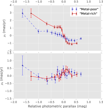
Figure 8. Variation of proper-motion centroid with relative photometric parallax, for "metal-rich" (red triangles) and "metal-poor" (blue circles) samples, using a binning scheme with 200 objects per bin. The top row shows the proper-motion centroid in Galactic longitude; the bottom row shows the proper-motion centroid in Galactic latitude. Error bars show 1σ uncertainties from parametric bootstrapping, using the best-fit parameters and measurement uncertainties to generate 1000 trial data sets for each distance bin. See Section 4.1.
Download figure:
Standard image High-resolution image4.1. Distance Conversion and Rotation Curves for the "Metal-rich" and "Metal-poor" Samples
Figure 11 presents the rotation and dispersion curves of the "metal-rich" and "metal-poor" samples expressed in terms of  . The conversion of these quantities from the measured (
 ) requires the reference distance
  corresponding to the fiducial sequences for the two samples. The reference distance was set by taking literally the distance modulus (m − M)0 = 14.45 suggested by studies of the SWEEPS CMD (Ca14), which in turn suggests reference distance (
 ). We assigned this reference distance to both the "metal-rich" and "metal-poor" samples (a choice we examine critically in Section 5.4).
Consistent with the simple treatment in Figure 7 and Section 3.6, the "metal-rich" sample shows a higher-amplitude rotation curve than does the "metal-poor" sample, with both a steeper slope and about a factor of ∼2 greater difference in mean transverse velocity  between the near side and far side of the bulge than for the "metal-poor" sample.
To quantify the rotation curve discrepancies between the samples, a simple straight-line model was fit to their rotation curves for distances close to the fiducial for each sequence. This interval was estimated separately for the two samples since their rotation curves appear to level off at different distances from the fiducial (Figure 11). For the "metal-rich" sample the gradient was estimated over the interval  in the (
 ,
,  ) curve (corresponding to −0.24 mag ≲
  ≲ +0.21 mag). The rotation curve of the "metal-poor" sample remains sloped over a broader range, so the fitting interval
  ± 1.4 kpc was used (so −0.44 mag ≲
  ≲ +0.36 mag). For both samples the rotation curve amplitude was estimated from the intervals where the rotation curves level off, covering two to three bins each outside the sloped region (Figure 12 indicates the regions used to estimate the rotation curve slopes and amplitudes). The 1σ ranges of
  and
and  from the parametric bootstrap trials were used as estimates of measurement uncertainty in each distance bin, and the trends were fitted to each of the (
 ,
,  ) and (
 ,
,  ) rotation curves separately (rather than transforming the proper-motion trends into velocity trends after fitting). We did not attempt to deproject velocities to circular speeds (as discussed in Cl08) but merely attempted to characterize observed trends.
Figure 12 and Table 7 show the results. The ratio of the gradients  was found to be
  =
=  , while the ratio of amplitudes
  is
is  =
=  . Thus, a ratio in rotation curve slopes was detected at approximately
  , while for the velocity amplitude the ratio was detected at roughly
  .
.
Table 7. Trend Parameters for the Inner Bulge Region
| Sample | Gradient (μl) | Amplitude (μl) | Gradient (vl) | Amplitude (vl) |
|---|---|---|---|---|
| (mas yr−1 mag−1) | (mas yr−1) | (km s−1 kpc−1) | (km s−1) | |
| "Metal-poor" (MP) | −1.78 ± 0.23 | 0.48 ± 0.07 | −18.6 ± 2.66 | 18.3 ± 2.58 |
| "Metal-rich" (MR) | −6.85 ± 0.73 | 1.16 ± 0.07 | −68.9 ± 8.04 | 41.9 ± 2.52 |
| MR–MP | −5.07 ± 0.77 | 0.68 ± 0.10 | −50.3 ± 8.5 | 23.6 ± 3.6 |
| MR/MP | 3.85 ± 0.64 | 2.42 ± 0.38 | 3.70 ± 0.68 | 2.29 ± 0.35 |
Note. See Section 4.1.
Download table as: ASCIITypeset image
The rotation curves in Galactic latitude (Figure 8, bottom panel) visually suggest gentle trends from near side to far side, consistent with previous measurements (e.g., Cl08, Soto et al. 2014). Table 8 reports the straight-line characterization of the Galactic latitude rotation curves, where here we characterized the trend as a straight-line fit within ±2.0 kpc from the fiducial distance  . The behaviors of the two samples in μb are statistically similar, with gradient ratio
  =
=  . We do not consider this to represent a secure detection of differing rotation curves in the direction of Galactic longitude.
Table 8.
Gradient of Straight-line Fits in Galactic Latitude, for Stars within ±2.0 kpc of the Fiducial Distance  Adopted in This Work
| Sample | Gradient (μl) | Gradient (vl) |
|---|---|---|
| (mas yr−1 mag−1) | (km s−1 kpc−1) | |
| "Metal-poor" (MP) | 0.26 ± 0.25 | 4.2 ± 2.76 |
| "Metal-rich" (MR) | 0.24 ± 0.28 | 3.8 ± 2.65 |
| MR–MP | −0.02 ± 0.38 | −0.4 ± 3.8 |
| MR/MP | 0.92 ± 1.40 | 0.90 ± 0.87 |
Note. See Section 4.1.
Download table as: ASCIITypeset image
4.2. Proper-motion Ellipse Morphology and Amplitudes
The velocity dispersion profiles (measured as major- and minor-axis lengths of the proper motion and velocity ellipsoids; Figures 9 and 11) also show differences between the samples. Both samples show a broadly centrally peaked velocity dispersion pattern against line-of-sight distance (Figure 11), with the "metal-rich" sample showing a narrower peak, particularly in the major-axis dispersion. The "metal-rich" sample also shows generally lower velocity dispersion by ∼10%, particularly in terms of the velocity ellipse minor axis.
Figure 9. Semimajor (top) and semiminor (bottom) axis lengths for the proper-motion ellipse. Symbols, colors, and error bars as for Figure 8. See Section 4.1.
Download figure:
Standard image High-resolution imageConsistent with previous studies (e.g., Soto et al. 2014), the proper-motion ellipse appears to be weakly elongated, with the "metal-rich" population possibly the more elongated of the two samples (with axis ratio  at
at  = 0 compared to
  see the top panel of Figure 10). However, the two axis-ratio trends show considerable bin-to-bin scatter.
Figure 10. Variation of the proper-motion ellipse axis ratio (top) and the position angle of its major axis (bottom) as a function of relative photometric parallax. Position angle θ = 0° would mean that the proper-motion ellipse major axis aligns with the Galactic longitude axis. Symbols as in Figure 8, with the "metal-poor" sample shown more faintly to avoid cluttering the plots. See Section 4.1.
Download figure:
Standard image High-resolution imageThe proper-motion ellipse major-axis position angle also shows trends with relative photometric parallax, although possibly at lower statistical significance than the trends reported in Cl08 despite a much longer time baseline for proper motions (Ca14). This reduced significance may be due to the reduced sample size admitted by the cuts in ![$[t],[m]$](https://content.cld.iop.org/journals/0004-637X/858/1/46/revision1/apjaaba7fieqn157.gif) employed in this work. It may be that only the "metal-rich" sample substantially shows the proper-motion ellipse tilt with distance, with position angle rising to the 20°–40° range (this tilt is strongly influenced by projection effects; see Section 5.1 and particularly Equation (2) of Cl08). Because the "metal-poor" population tends to be less elongated, its position angle trends are also detected at lower significance.
employed in this work. It may be that only the "metal-rich" sample substantially shows the proper-motion ellipse tilt with distance, with position angle rising to the 20°–40° range (this tilt is strongly influenced by projection effects; see Section 5.1 and particularly Equation (2) of Cl08). Because the "metal-poor" population tends to be less elongated, its position angle trends are also detected at lower significance.
The very nearest relative photometric parallax bins show behavior consistent with a foreground population dominated by Galactic rotation. This seems particularly clear for the "metal-rich" sample, which shows a much more strongly elongated proper-motion ellipse for the nearest bin ( ) and position angle consistent with zero (consistent with differential rotation in Galactic latitude).
5. Discussion
The trends indicated by the union of the BTS and SWEEPS data sets, particularly the rotation curves (presented in Figures 7, 8, and 11), are quite striking. The "metal-rich" rotation curve appears to show systematically greater rotation amplitude than the "metal-poor" sample, shows a greater degree of central concentration along the line of sight (see Figure 11, as well as the raw distributions in Figure 6), and, with the exception of the middle distance bins, may show systematically lower velocity dispersion (Figure 11).
Figure 11. Transverse velocity ellipse centroids (left column) and axis lengths (right column) as a function of estimated line-of-sight distances. Symbols as in Figures 8 and 9, except distance moduli have been converted to line-of-sight distances and proper motions converted to velocities in km s−1. See Section 4.1.
Download figure:
Standard image High-resolution image
Figure 12. Straight-line fits to the inner region of the longitudinal rotation curve along the line of sight, after conversion to velocities and physical distances. The comparison sequences for both samples are assumed to lie at distance  . The filled regions indicate ±1.0σ regions for each sample. The horizontal shaded regions show the intervals assumed to be "flat" to estimate the rotation amplitude for each sample. See Section 4.1 and Table 7.
Download figure:
Standard image High-resolution imageBefore attempting to interpret the trends, however, we examine the magnitude and impact of several potential systematics that might bias the samples, whether by amplifying or even artificially generating the apparent differences in rotation curve (Section 5.1), or by reducing them as a result of mixing in the (![$[t],[m]$](https://content.cld.iop.org/journals/0004-637X/858/1/46/revision1/apjaaba7fieqn160.gif) ) space used to draw the "metal-rich" and "metal-poor" samples (Section 5.2). The impact of extinction variations along the line of sight, including additional extinction on or past the far side of the bulge, is discussed in Section 5.3. Systematic uncertainties in the final velocity rotation curves due to the proper-motion zero-point and fiducial distance are discussed in Section 5.4.
) space used to draw the "metal-rich" and "metal-poor" samples (Section 5.2). The impact of extinction variations along the line of sight, including additional extinction on or past the far side of the bulge, is discussed in Section 5.3. Systematic uncertainties in the final velocity rotation curves due to the proper-motion zero-point and fiducial distance are discussed in Section 5.4.
In Section 5.5 we address the question whether the bulge rotation curve from proper motions indeed depends on relative abundance, and we briefly assess trends in proper-motion dispersion in Section 5.6. Implications of the relative photometric parallax distributions for the spatial distributions of the "metal-rich" and "metal-poor" samples are discussed in Section 5.7. Because a metal-poor kinematically hot "classical bulge" and/or "halo" bulge component may be present in the inner Milky Way (perhaps more likely among "metal-poor" objects), we attempt in Section 5.8 to dissect each of the "metal-rich" and "metal-poor" populations into two proper-motion components per sample. Finally, Section 5.9 discusses the implications of our results for the traditional selection of a "clean-bulge" sample using cuts on longitudinal proper motion  .
.
5.1. Difference Amplification by Photometric Parallax Mixing
Differences in apparent magnitude distribution other than those due to distance spread would contribute to differences in the inferred  distributions for the "metal-rich" and "metal-poor" samples. If sufficiently severe, this differential blurring in
  might cause two intrinsically identical rotation curves to be erroneously measured as discrepant. In the sense of our findings, the "metal-poor" sample might be artificially blurred in
  compared to the "metal-rich" sample, which would produce an apparent rotation curve discrepancy where none were present.
Several phenomena might lead the "metal-poor" sample to exhibit greater apparent magnitude scatter than the "metal-rich" sample. First, since the "metal-poor" ridgeline in the SWEEPS CMD is slightly fainter than the "metal-rich" ridgeline, the "metal-poor" objects may be subject to increased photometric uncertainty. Second, at least in principle, if the extinction distribution experienced by the two samples were in some way different, this could lead to a broader apparent magnitude distribution for the "metal-poor" sample. Third, differences in binary fraction between the samples might cause the relative photometric parallax distribution of the two samples to differ, although the nature, magnitude, and direction of such effects may be complex and indeed depend on the class of binaries probed (e.g., Gao et al. 2014).
Finally, differences in the intrinsic photometric scatter between the "metal-rich" and "metal-poor" samples might amplify differences between the rotation curves. Our own VLT spectroscopy, as well as spectroscopic campaigns from the literature (e.g., Hill et al. 2011; Zoccali et al. 2017), suggests that the [Fe/H] spread for the "metal-poor" population is greater than for the "metal-rich" population, which would in turn contribute greater  scatter in the "metal-poor" population.
We have performed simple Monte Carlo tests to determine whether perturbations in the inferred distance distribution can be responsible for the differences in rotation curves between "metal-rich" and "metal-poor" samples. Appendices D and E provide details.
In the course of investigating the impact of the differential [Fe/H] distribution on the  distribution, it became apparent that the BaSTI set of artificial stellar population methods used to generate synthetic [Fe/H] distributions was (at the time of this work) imposing an apparently artificial population truncation. Appendix F provides details, with the method we adopted to mitigate this selection effect discussed in Appendix E.
Perturbations were tested as a result of additional photometric uncertainty or differential extinction variations (Appendix D.1), differences in the fraction of unresolved binaries (Appendix D.2), and differences in the photometric parallax spread caused by differing intrinsic spreads in metallicity (Appendix E). In all scenarios, either the effect is too small to bring the rotation curves into agreement (for binaries), or the required perturbation is too large to have gone unnoticed in previous studies (for extinction), possibly by an order of magnitude (for photometric uncertainty). The strongest single contributor of relative photometric parallax mixing is intrinsic difference in metallicity spread between the samples; this likely contributes differential distance mixing up to one-third the amount required to artificially reproduce the observed discrepancy in rotation curves. Since independent sources of additional photometric scatter would presumably add in quadrature, their combination is very unlikely to be sufficient to bring about the observed discrepancies in trends.
We therefore conclude that differential distance scatter is not responsible for the difference in rotation curves or  distributions, due to additional photometric uncertainty, differential extinction, differences in the unresolved binary populations, or differences in metallicity spread between samples.
5.2. Difference Reduction by Sample Cross-contamination
While blurring in relative photometric parallax would tend to artificially increase the difference between trends in the "metal-rich" and "metal-poor" samples, cross-contamination of the samples in (![$[t],[m]$](https://content.cld.iop.org/journals/0004-637X/858/1/46/revision1/apjaaba7fieqn168.gif) ) would tend to artificially reduce these differences. While we have used reasonably conservative thresholds in drawing our "metal-rich" and "metal-poor" samples, genuinely metal-rich objects might be moved into the "metal-poor" sample by measurement uncertainty, and vice versa.
) would tend to artificially reduce these differences. While we have used reasonably conservative thresholds in drawing our "metal-rich" and "metal-poor" samples, genuinely metal-rich objects might be moved into the "metal-poor" sample by measurement uncertainty, and vice versa.
Because of the complexities involved in rigorous reconstruction of the observed distributions (e.g., Gennaro et al. 2015), full exploration of this cross-contamination is deferred to future work. We have performed a simple Monte Carlo contamination test for the formal membership probability threshold  >
>  used in this work (Appendix G). Under the assumptions of that test, we find that the "metal-rich" sample is contaminated at the ∼5% level (mostly from the "metal-poor" sample), while the "metal-poor" sample is contaminated at the ≲1% level (mostly due to the "metal-rich" sample, but with some contribution from background component k = 3 in Table 5). This is not severe enough for the observed low-amplitude "metal-poor" rotation curve to be due to sample contamination from a small population of objects following the kinematics of the "metal-rich" sample.
5.3. Trend Modification by Line-of-sight Extinction Variations
Our treatment of the impact of extinction on the photometry (and therefore the relative photometric parallax) assumes that the extinction is constant over the line-of-sight distances of interest. Violations of this assumption might in principle influence the trends we observe, by artificially broadening the line-of-sight distribution (with stars more affected by extinction appearing farther from the observer).19 Here we examine the likely impact on our main results of extinction variations along the line of sight.
A few studies have mapped the 3D extinction distribution out to the far side of the bulge (e.g., Marshall et al. 2006; Schultheis et al. 2014). Particularly for sight lines close to the Sagittarius window we study here, most of the extinction at these distances takes place at distances  ≲ 5 kpc from the Sun, possibly broken into two foreground concentrations (at
  ≈ 3 and 5 kpc; e.g., Marshall et al. 2006). Thus, along our sight line, extinction variations within the bulge are likely to be small compared to variations in the foreground disk, an interpretation consistent with the photometry of red clump stars in this field (Cl08). Hence, the trends we find for line-of-sight distances 5 kpc ≲
  ≲ 11 kpc—the main sample of interest—are likely unaffected.
By symmetry we might expect additional extinction from at least one dust screen at distances  ≳ 11 kpc owing to spiral structure on the far side of the bulge (see, e.g., Figure 10 of Schultheis et al. 2014). This would be mitigated somewhat by the slightly tilted path of our line of sight compared to the Galactic plane; at Galactic latitude bJ2000.0 = −265, our sight line is already ≈480 pc below the Galactic midplane when it reaches
  = 11 kpc, roughly where it might intersect the first dust concentration on the far side of the bulge (compared to ≈210 pc at 5 kpc), suggesting that far-side extinction may likely be somewhat weaker than experienced in the foreground.
We therefore conclude that indeed the photometric parallaxes for objects closer than  ≈ 5 kpc and farther than
  may have been assigned photometric parallaxes that are artificially close and far, respectively. However, as those distances are outside our main regions of interest, this does not impact any of the trends that we report.
5.4. The Influence of the Proper-motion and Distance Zero-points
All proper motions in this work are reported relative to the same proper-motion zero-point  , which is defined as the average proper motion of astrometrically well-measured stars, whatever their metallicity (Section 2.1). We have chosen not to apply separate proper-motion zero-points to the two samples, for example, by forcing the two samples to each show
  = 0.0 mas yr−1 at
  = 0.0 mag, but opt to keep the proper motions in the same reference frame for each sample to allow direct comparison between (
 , μ) rotation curves.
We then find that the central proper motions for the "metal-rich" and "metal-poor" samples (i.e., the median proper motions for stars near their fiducial sequences) differ by  mas yr−1 (Section 3.6); equivalently, the rotation curves do not meet at (
 ,
,  ) = (0 mag, 0 mas yr−1).
These discrepancies could be due to differences in the mean intrinsic velocities of the fiducial stars between the samples, or differences in the line-of-sight distance at which the fiducual stars are found, or a combination of the two. Since the fiducial sequences for the two samples are determined from their CMD population densities (see Figure 5), their central proper motions could well differ if their densest observed regions occurred at different distances. This could occur naturally if the two samples are oriented differently in the Galactic plane (in which case the relationship between the mean velocity  and its transverse velocity components
  and
and  would also differ between the samples).
If the fiducial stars for the two samples do indeed lie at different distances  (with Δk giving the distance offset for a particular sample), then the appropriate conversion from (
 ,
,  ) to (
 ,
,  ) will also differ, in turn impacting the difference in rotation curve velocity amplitude for the two samples. Figure 13 shows how the velocity rotation curve is impacted by shifting the "metal-rich" fiducial by distance offset Δ kpc from the "metal-poor" fiducial. Bringing the "metal-rich" fiducial closer than the "metal-poor" one does reduce the velocity amplitude discrepancy between the two samples. However, to bring the velocity amplitudes of the two samples into agreement, the "metal-rich" fiducial would need to be brought closer by
  , which seems unlikely for samples so close to the Galactic rotation axis (at
  ). Unless the spatial distributions of the two samples really are radically different, then, we consider it unlikely that a difference in fiducial distance between the samples can by itself produce the observed difference in velocity rotation curve amplitude we are measuring.
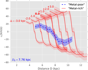
Figure 13. Estimation of the impact on the velocity rotation curves of allowing the fiducial distance to differ between the samples. The blue dashed line shows the velocity rotation curve of the "metal-poor" sample, converting from ( ,
,  ) to (
 ,
,  ) using fiducial distance
  (the shading encompasses
  uncertainties at each distance bin). The red solid lines show velocity rotation curves for the "metal-rich" sample, using fiducial distance
  + Δ. Reading left to right, the distance offset varies over the range −3.0 kpc ≤ Δ ≤ 3.0 kpc in 1 kpc increments. The case Δ = 0 is highlighted for reference. See Section 5.4.
Download figure:
Standard image High-resolution imageWhile an offset Δ in fiducial distance scales the velocity amplitude by a corresponding amount, an offset  in the proper-motion zero-point produces a systematic shift
  in the velocity gradient. If
  (the average proper motion of well-measured bulge stars of all metallicities) and
  (the average distance to bulge stars of all metallicities) are both determined from the same set of stars, then we would have
  = 0 mas yr−1 and thus
  = 0
= 0  .
.
However, in reality the sets of stars used to estimate  and
and  will in general differ. The fiducial distance
  is estimated from the distribution of "extreme-bulge"(EB) stars showing
  mas yr−1 (e.g., Ca15), while
  is estimated from stars below the MS turnoff without any proper-motion selection. Thus, although stars well measured astrometrically tend also to be well measured photometrically, differing selection effects in the determination of
  and
and  will still lead to a global systematic offset in
  .
.
The true value of  is unknown; however, we can form a rough estimate as the median proper motion of the population traced by the EB objects used to estimate
  (Ca14). The EB objects have highly negative proper motions by construction, but we can estimate the median proper motion of the underlying population that they trace by estimating the median photometric parallax
  of the EB tracers and applying the proper-motion rotation curve characterization
  of Section 4.1. Since we have performed this characterization separately for "metal-rich" and "metal-poor" samples, we can estimate
  separately from the two samples. Applying the kinematic cut
  ≤ −2.0 mas yr−1 to extract EB tracers for the "metal-rich" and "metal-poor" populations, we find median photometric parallax
  ≈ +0.025 mag and
  ≈ −0.002 mag for EB objects in the "metal-rich" and "metal-poor" samples, respectively (so that objects with
  = 0 mas yr−1 lie slightly in front of the EB population, as expected; see Section 5.9). This suggests that the underlying population traced by the EB objects—corresponding to the fiducial distance
  —has median longitudinal proper motion
  mas yr−1. These figures are likely also sensitive to differing intrinsic proper motion and distance distributions between the samples, but this estimate suggests that the proper-motion difference between the sample from which the proper-motion reference frame was set and the sample from which
  was estimated is not larger than
  ≲ 0.17 mas yr−1. Thus, the systematic velocity gradient uncertainty
  may be on the order of ∼
 .
.
Systematic uncertainty in the proper-motion zero-point  may therefore impact the ratio of longitudinal velocity gradients reported in Section 4.1 by ≲10% (Table 7), which is too small to materially affect the main results or conclusions we report.
5.5. Does the Proper-motion Rotation Curve Vary with [Fe/H]?
We are finally in a position to answer the question posed by Section 1.1. Our "metal-rich" and "metal-poor" rotation curves are inconsistent with each other at  for the rotation curve slope and
  for the near-side−far-side rotation amplitude (Section 4.1).
These proper-motion-based results stand in strong contrast to determinations of the radial velocity rotation trends, which either find weak if any discrepancy between "metal-rich" and "metal-poor" samples (e.g., Ness et al. 2013b; Williams et al. 2016; Zoccali et al. 2017) or require a large contribution from samples with [Fe/H] < −1.0 to produce a discrepancy in rotation curves (e.g., Minniti 1996; Kunder et al. 2016; note that the fraction of stars in our sight line with [Fe/H] < −1.0 is likely low; Zoccali et al. 2017). It seems unlikely that this discrepancy between our proper-motion-based study and these radial-velocity-based studies can be due purely to any differences between the uses of giant and dwarf stars as tracers, since microlensed dwarf stars also show no strong differences in mean radial velocity between metal-poor and metal-rich stars (or, for that matter, between stars younger and older than ∼7 Gyr; Bensby et al. 2017).20
The most likely explanation for the difference between proper-motion and radial velocity results is the strong difference in the way the studies sample the inner Milky Way. Detailed comparison of our new observational indications with model prediction is deferred to future work; however, a likely scenario to explain the differences can be outlined as follows. In the simulations of Debattista et al. (2017), the final orbital configuration of bulge stars depends on their (radial) velocity dispersion before bar formation. To the extent that [Fe/H] and radial velocity dispersion correlate with each other (or, equivalently, each correlate with time of formation), the "kinematic fractionation" resulting from bar formation might well leave metal-rich stars with a higher fraction of elongated orbits than for metal-poor objects. That the "X" structure is observed to preferentially contain metal-rich objects (e.g., Vásquez et al. 2013) supports the notion that stars within our "metal-rich" and "metal-poor" samples on average move along differently shaped orbits, while the spatial structures traced by Mira variables of different pulsation period ranges suggest that samples with differing spatial configuration can coexist in the same volume at the present day (Catchpole et al. 2016). The "metal-rich" and "metal-poor" samples may then show quite different transverse velocity distributions as a function of line-of-sight distance, even if the distributions produce similar mean velocities when averaged along the line of sight owing to radial velocity survey selection effects. In this scenario, only by dissecting the population by line-of-sight distance (or its proxy,  ) can the differing velocity distributions of the two coexisting samples be distinguished.
Since stars in the "metal-rich" and "metal-poor" samples all move through the same present-day potential, by detecting differences in the proper-motion-generated rotation curve, we may well be detecting differences in orbital anisotropies between metal-rich and metal-poor bulge objects. While detailed prediction is a topic of ongoing work, the differences we detect seem qualitatively reasonable at present.
Having shown that the proper-motion-based rotation curve does show discrepancy between "metal-rich" and "metal-poor" populations, the necessary next step is to extend our approach to more sight lines within the inner bulge. By comparing metallicity-dissected proper-motion-based rotation curves between fields, the trends with location in the bulge can be charted empirically, allowing a sharper test of the true variation of bulge rotation with the metallicity of the sample probed. This work is deferred to a future communication.
5.6. Proper-motion Dispersion Trends with Photometric Parallax
Both the "metal-rich" and "metal-poor" samples show a clear central peak in velocity ellipse major-axis length near the distance interval where the samples are the most densely populated (Figure 11). The peak persists in the velocity ellipse minor axis for the "metal-rich" sample but is rather less clear in the "metal-poor" sample. This is broadly similar to the trends found from the combined population in previous studies (e.g., Cl08, Soto et al. 2014). We note a rough, qualitative similarity with the curve of radial velocity against Galactic longitude for Galactic latitude b = −2° (see the middle left panel of Figure 12 of Zoccali et al. 2017); however, we remind the reader that the radial velocity and proper-motion trends cannot directly be compared because they suffer from differing selection effects. That the proper-motion dispersion of the "metal-poor" component is generally slightly larger than that of the "metal-rich" one (particularly along the minor axis) is qualitatively consistent with expectations that a metal-poor, less rotationally supported population should show higher velocity dispersion (e.g., Ness et al. 2013b; Debattista et al. 2017).
We may also be detecting the velocity dispersion "inversion" detected at the innermost fields in radial velocity studies (Babusiaux et al. 2014; Zoccali et al. 2017). Consistent with the low-latitude radial velocity dispersion trends, the proper-motion-based velocity dispersion might also be greater for the "metal-rich" sample than for the "metal-poor" sample at the distance bins closest to the center of the bulge (see Figure 11). For the innermost bulge regions, the proper-motion-based "metal-rich" velocity dispersions also show steeper gradient than the "metal-poor" ones, but with the gradient against line-of-sight distance rather than Galactic longitude, with the innermost distance bin possibly showing slightly greater velocity dispersion for the "metal-rich" sample.
5.7. The Line-of-sight Distance Distributions of the Two Samples
The tendency of the "metal-poor" sample to show greater dispersion in relative photometric parallax (or, correspondingly, in distance  ) is qualitatively consistent with the "kinematic fractionation" of Debattista et al. (2017). Under that mechanism, more "metal-poor" populations also initially had greater radial velocity dispersion, leading to a distinct (and broader) present-day spatial distribution when compared to the most "metal-rich" objects.
The difference we find in line-of-sight distribution between the "metal-rich" and "metal-poor" samples might also be consistent with the observations of Catchpole et al. (2016), who find differing bar angles and degrees of central concentration for Mira variables of different ages. However, the interplay between age and metallicity of bulge stars is likely not simple. For example, while a gentle relationship may exist between [Fe/H] and the fraction of stars younger than about 8 Gyr (e.g., Figure 14 of Bensby et al. 2017 or Figure 10 of Bernard et al. 2018), the microlensing spectroscopic surveys suggest that stars can take any metallicity value (for [Fe/H] ≳ −1.0) for any age. How the predictions of Catchpole et al. (2016) translate into predictions for the two samples here is deferred to future work.
5.8. Are the Metallicity Samples Themselves Composite?
In addition to any continuous metallicity–velocity correlation, the samples may include populations from distinct entities within the bulge region, whether interlopers from the halo (e.g., Koch et al. 2016), any thick-disk component (e.g., Ness et al. 2013a), or a small "classical" bulge component (Kunder et al. 2016).
We have therefore performed the exercise of decomposing each of the "metal-rich" and "metal-poor" samples into two-component GMMs (in  only), to determine whether any minority component is distinguishable within the rotation curves formed from the two samples (Figures 14 and 15). No minority population is detected in either sample; indeed, when a two-component GMM is used, the two centroids track the mean rotation curve within each sample roughly symmetrically about the mean rotation curve, while each subcomponent has roughly equal weight in the mixture.
Figure 14. Representation of the "metal-poor" rotation curve as a two-component GMM in  , to test the hypothesis that the "metal-poor" sample might itself be composite. Left column: rotation curve in
  as tracked by the two model components (top), and the relative weights of the two model components (bottom). Large dots indicate the more populous of the two model components in each bin (αk = 0.75 would mean that three-quarters of the sample came from model component k). The gray line in the top left panel shows the rotation curve inferred using a single model component at each distance bin. Right column:
  distribution for the bin indicated for the shaded distance bin in the left column. Top right:
  distribution (shaded histogram and thin black line), with the prediction of the two-component GMM (the thick and thin blue lines indicate the more and less populous model component, respectively, while the blue dashed line indicates the sum of the two). The gray thick line shows the prediction of the single-component model. The bottom left and bottom right panels show the vector point diagram and distance modulus distribution, respectively. See Section 5.8.
Download figure:
Standard image High-resolution image
Figure 15. Representation of the "metal-rich" rotation curve as a two-component GMM in  , to test the hypothesis that this sample might be a composite of two subpopulations. Symbols similar to Figure 14, except red symbols and lines are substituted for blue. See Section 5.8.
Download figure:
Standard image High-resolution imageWe therefore conclude that a minority component with discrepant rotation curve is not required in either the "metal-rich" or "metal-poor" sample, but due to the small sample size (≈2000 stars in total per sample), we cannot at this stage rule out its presence. Direct comparison with population models may allow upper limits to be set on the presence of any minority component within each sample, but this is deferred to future work.
5.9. Implications for Proper-motion Selection
Photometric studies of the bulge typically impose a condition  mas yr−1 to isolate a clean-bulge sample for further study (e.g., Kuijken & Rich 2002; Calamida et al. 2014), although there are exceptions (e.g., Bernard et al. 2018).21
This procedure is appropriate because in the sight lines typically studied near the Galactic center the foreground disk population typically shows proper motion relative to the mean-bulge population of Δμl ≈ +4 mas yr−1, as suggested by direct comparison of the proper motions of bulge giant branch stars with those of the upper MS population of (mostly) disk foreground stars (e.g., Cl08; Soto et al. 2014).
mas yr−1 to isolate a clean-bulge sample for further study (e.g., Kuijken & Rich 2002; Calamida et al. 2014), although there are exceptions (e.g., Bernard et al. 2018).21
This procedure is appropriate because in the sight lines typically studied near the Galactic center the foreground disk population typically shows proper motion relative to the mean-bulge population of Δμl ≈ +4 mas yr−1, as suggested by direct comparison of the proper motions of bulge giant branch stars with those of the upper MS population of (mostly) disk foreground stars (e.g., Cl08; Soto et al. 2014).
To investigate whether and how a simple cut on  imposes selection effects on the two samples, we computed the sample counts, fractions, and volume densities for objects that would pass the longitudinal proper-motion cut (μl < −2.0 mas yr−1). The results are plotted in Figure 16 and presented in tabular form in Tables 16 and 17 in Appendix I.
Figure 16. Selection functions imposed by the traditional kinematic cut μl ≤ −2.0 mas yr−1, for the "metal-rich" (red triangles, solid line) and "metal-poor" (blue circles, dashed line) samples.Left column: volume density of all objects assigned to each sample (top) and which would pass the kinematic cut (bottom). Right column: number of objects per sample that would pass the kinematic cut (top) and the fraction (bottom) that would pass the cut. Each distance bin has the same number of detected objects by construction (Section 3.7), so bootstrap uncertainty estimates are not applicable to the top left panel. Because of this binning scheme, bins with the same counts generally do not indicate the same volume density of detected objects (between bins or between samples). The shaded yellow region represents inferred distances 6.5 kpc ≤ d ≤ 9.0 kpc. For discussion, see Section 5.9.
Download figure:
Standard image High-resolution imageWe find that the cut (μ < −2.0 mas yr−1) admits very few foreground objects from either sample; both samples show fewer than two objects passing this cut for the closest distances ( and ≲4.10 kpc for "metal-rich" and "metal-poor" samples, respectively; see Tables 16 and 17 in Appendix I), while the mean proper motion
  of the foreground population climbs strongly for the closest distance bins (Figure 8). We therefore confirm that the traditional proper-motion cut (μ < −2.0 mas yr−1) does indeed remove nearby objects cleanly for the SWEEPS field.22
Beyond this, however, the dissection by relative abundance has revealed several interesting selection effects among the kinematically cleaned sample (Figure 16).
First, as expected, there is a bias toward the far side of the bulge, but this bias is much stronger in the "metal-rich" sample than for the "metal-poor" one; indeed, the fraction of "metal-poor" objects passing the kinematic cut is almost flat with inferred distance between ~5 and 9 kpc.
Second, the raw counts of sources thus isolated in the "metal-rich" and "metal-poor" samples are of similar orders of magnitude. Considering sample sizes that pass the kinematic cut at inferred distances between 6.4 and 9.1 kpc (chosen to encompass the bulge populations; see Tables 16 and 17), the total counts in each sample are 521 ± 19 and 507 ± 19 for the "metal-rich" and "metal-poor" samples, respectively (the uncertainties, estimated from the quadrature sum of parametric bootstrap uncertainty estimates in these counts for each bin, are almost certainly underestimates). With total sample sizes within this distance range of 2181 (1783) for the "metal-rich" ("metal-poor") samples, this translates into fractions 24% ± 1% (28% ± 1%) of the "metal-rich" ("metal-poor") samples that pass the kinematic cut. Thus, of objects in this distance range, the kinematic cut appears to slightly favor the "metal-poor" sample, although the difference is small.
In principle, a population of compact objects among the foreground population might fall into the farther distance bins for the "metal-poor" sample,23 polluting a sample with bulge-like motions with a small population showing disk-like motions. However, with the foreground disk population at ∼10% of the total (Ca14) and with a substantial white dwarf population perhaps unlikely for a typical "young" foreground population, we do not consider this a significant contaminant, and we leave exploration of the impact of foreground white dwarfs to future work.
6. Conclusions
We have performed an exploratory study to determine the utility of HST proper motions in charting the kinematic behaviors of "metal-rich" and "metal-poor" samples within the Galactic bulge from their proper motions, extending the rotation curve technique first pioneered by Kuijken & Rich (2002). The ultradeep SWEEPS photometric and astrometric data set communicated in Calamida et al. (2014) was merged with the WFC3 Galactic Bulge Treasury Survey (Brown et al. 2010); "metal-rich" and "metal-poor" samples were drawn using the ![$[t],[m]$](https://content.cld.iop.org/journals/0004-637X/858/1/46/revision1/apjaaba7fieqn249.gif) indices of Brown et al. (2009), recomputed for the stellar parameters appropriate to the proper-motion sample of interest and assuming
indices of Brown et al. (2009), recomputed for the stellar parameters appropriate to the proper-motion sample of interest and assuming  . The proper-motion-based rotation curves were determined from the "metal-rich" and "metal-poor" samples separately, using relative distance modulus as the depth coordinate. While detailed comparison to population models is deferred to future work, we draw the following conclusions at present:
- 1.The union of SWEEPS and BTS data sets has revealed that indeed the "metal-rich" and "metal-poor" rotation curves are clearly discrepant from each other.
- 2.Characterizing the rotation curves for the inner bulge regions with straight-line fits, the "metal-rich" population shows a steeper rotation curve in Galactic longitude, with gradient ratio
 = (a ≈ detection).
 - 3.The near-side−far-side velocity amplitude is also determined to be discrepant; the rotation curve amplitude of the "metal-rich" sample is greater than that of the "metal-poor" sample by a factor = (a ≈ detection).
- 4.While selection effects are likely complex, it does not appear to be possible to force the rotation curve of the "metal-rich" sample into consistency with that of the "metal-poor" sample by any reasonable observational perturbation of the "metal-rich" sample. Therefore, the differences in rotational behavior likely represent intrinsic behavior, not instrumental or observational artifacts.
- 5.The velocity dispersion curve of both samples shows a clear peak at the line-of-sight distance where the samples are most dense. At the innermost distance bins, the velocity dispersion of the "metal-rich" sample shows a steeper gradient than does the "metal-poor" sample, consistent with recent radial velocity studies.
- 6.These results may indicate differences in orbital anisotropy between metal-rich and metal-poor objects within the bulge, in turn providing a new observational criterion for testing models of bulge formation and evolution.
- 7.The traditional proper-motion cut used to isolate a clean-bulge sample, μl < −2.0 mas yr−1, slightly overselects "metal-poor" objects compared to "metal-rich" ones, at the level of 28% compared to 24%.
- 8.However, this selection effect is a function of relative photometric parallax; with this cut, the fraction of "metal-poor" objects selected is roughly constant, while for the "metal-rich" population the selection strongly prefers objects on the far side of the bulge.


In addition, while exploring population systematics, we have found the following:
- 1.The current version (v5.0.1) of the widely used BaSTI set of synthetic stellar population methods and isochrones appears to be imposing a truncation on populations near the edges of the [Fe/H] distribution found in the bulge; this includes a large part of the metallicity range traced by stellar halo models (e.g., An et al. 2013). Studies using BaSTI version 5.0.1. or earlier may be vulnerable to this truncation.
The Galactic bulge thus joins the list of stellar populations suspected to show distinct rotation curves depending on the chemistry of the tracer stars used, including at least one globular cluster (M13; Cordero et al. 2017) and the Sculptor dwarf spheroidal galaxy (e.g., Zhu et al. 2016, and references therein).
While the SWEEPS data set represents the deepest (by far) set of images ever taken by HST toward the inner bulge, the typical apparent magnitude range probed by this study is shallow enough that we expect the techniques presented herein to be applicable to other fields for which (![$[t],[m]$](https://content.cld.iop.org/journals/0004-637X/858/1/46/revision1/apjaaba7fieqn258.gif) ) are available. The extension of this work to the other fields in the BTS survey is deferred to a future communication. This will provide a relatively assumption-free set of observational constraints against which the trends from the most recent set of models can be compared, subjecting them to direct test. This will finally enable the Galactic bulge to be used as a quantitative test case for the formation and development of galactic structure.
) are available. The extension of this work to the other fields in the BTS survey is deferred to a future communication. This will provide a relatively assumption-free set of observational constraints against which the trends from the most recent set of models can be compared, subjecting them to direct test. This will finally enable the Galactic bulge to be used as a quantitative test case for the formation and development of galactic structure.
This work made use of the Hubble Legacy Archive, which is a collaboration between the Space Telescope Science Institute (STScI/NASA), the Space Telescope European Coordinating Facility (ST-ECF/ESA), and the Canadian Astronomy Data Centre (CADC/NRC/CSA). Support for programs 9750, 11664, 12020, 12586, and 13057 was provided by NASA through grants from STScI, which is operated by AURA, Inc., under NASA contract NAS 5-26555. This work is partly based on observations collected at the European Organisation for Astronomical Research in the Southern Hemisphere under ESO program 073.C-0410(A).
This work has made use of data from the European Space Agency (ESA) mission Gaia (https://www.cosmos.esa.int/gaia), processed by the Gaia Data Processing and Analysis Consortium (DPAC, https://www.cosmos.esa.int/web/gaia/dpac/consortium). Funding for the DPAC has been provided by national institutions, in particular the institutions participating in the Gaia Multilateral Agreement.
W.I.C. acknowledges support from the University of Michigan–Dearborn through startup funding from the Department of Natural Sciences (project U039878) and from the Office of Research and Sponsored Programs (project U042549, The Milky Way Bulge at UM-Dearborn), partial support from HST program GO-12020 (PI Clarkson), and equipment funding from a Theodore Dunham Jr. Grant from the Foundation Center (award 1179, project N017429). V.P.D. is supported by STFC Consolidated grant ST/M000877/1. D.M. and M.Z. acknowledge support by the Ministry of Economy, Development, and Tourism's Millennium Science Initiative through grant IC120009, awarded to The Millennium Institute of Astrophysics (MAS); by Fondecyt Regular grants 1170121 and 1150345; and by the BASAL-CATA Center for Astrophysics and Associated Technologies PFB-06.
All the external software packages and methods used in this work are freely available to the community. This research made use of Astropy, a community-developed core Python package for Astronomy. This work made use of the astroML suite of tools for machine learning in Astronomy. This work made use of scikit-learn. This work has made use of the pysynphot synthetic photometry utilities. This work has made use of BaSTI web tools.
W.I.C. thanks Jay Anderson, Jo Bovy, Dana Casetti-Dinescu, Oscar Gonzalez, Noé Kains, Andreas Koch, Vera Kozhurina-Platais, and Laura Watkins for enlightening interaction at various stages of this analysis. This work was only possible thanks to the distortion solution and astrometric measurement methods developed by Jay Anderson. We thank Santi Cassisi for assistance with the BaSTI synthetic stellar population tools and for kindly providing custom synthetic populations at high metallicity.
Finally, we thank the anonymous referee, whose thorough reading and insightful comments led to substantial improvement of the manuscript.
Facilities: HST(ACS) - Hubble Space Telescope satellite, HST(WFC3) - Hubble Space Telescope satellite, VLT(UVES). -
Software: Astropy (The Astropy Collaboration et al. 2018),24 scikit-learn (Pedregosa et al. 2011),25 astroML (Ivezić et al. 2014),26 BaSTI (Pietrinferni et al. 2004),27 pysynphot (STScI Development Team 2013).28
Appendix A: SWEEPS Proper-motion Measurement Uncertainty
Proper-motion uncertainties from the 2004–2013 SWEEPS data are impacted by random uncertainties, by intrinsic velocity dispersion of the objects used to fit frame transformations when estimating proper motions, and by residual relative distortion between epochs. Here we discuss these sources of uncertainty in turn.
As part of the investigation of the faintest detectable objects in the SWEEPS field, Ca15 performed extensive artificial-star tests, including the injection of proper motions across the entire set of 2004–2013 epochs, yielding the run of random proper-motion uncertainty in each coordinate with apparent magnitude, which we denote here as  . While Ca15 thus produced separate estimates for uncertainties in the detector-X and detector-Y directions, for the apparent magnitude range of interest to this work the characterizations in the two directions are similar; in practice, we use the two runs in detector-X and detector-Y as separate samples of a symmetric underlying uncertainty distribution, characterizing log10(ξ) as a fifth-order polynomial in F814W for rapid evaluation.
Improved characterization of residual distortion has also become available, as the data sets used to characterize ACS/WFC distortion have grown. In the SWEEPS filters, residual distortion is on the order of ≈0.01–0.02 ACS/WFC pixels (0.5–1.0 mas at ≈50 mas pixel−1), with a complex pattern of variation with spatial scale roughly 150 ACS/WFC pixels (Anderson & King 2006; Kozhurina-Platais et al. 2015). This is consistent with a recent high-precision astrometric characterization of the full set of SWEEPS epochs for astrometric microlensing (Kains et al. 2017), which indicated residual distortion corrections of ≈±0.02 ACS/WFC pixels for the candidate astrometric microlensing sources (evaluated within 200 ACS/WFC pixels of each candidate; see Kains et al. 2017 for details), with the residual changing sign seasonally owing to the midyear 180° flip in HST's orientation angle for observations of this field. The observation dates of the 2011–2012–2013 epoch sample both HST orientations roughly equally, so the residual distortions in this epoch were to some extent averaged through when mean positions were computed per star, while central pointings in this epoch are typically within ∼50 ACS/WFC pixels of the central pointing of the 2004 epoch. We therefore adopt Δ ≈ 0.015 pixels (0.75 mas) as a reasonable estimate for the differential residual distortion suffered when proper motions are estimated across the two epochs.
For each object, then, the per-coordinate proper-motion uncertainty  i can be estimated from the relation

where  is the artificial-star-test random proper-motion uncertainty estimate evaluated at the apparent magnitude of the object. Ntr is the number of tracer stars used to map the reference frames between epochs, and σpm is the proper-motion dispersion (in mas yr−1) of the tracer stars (assumed to be estimated from the observed data, although if Ntr is large, this assumption has little effect).29
τ is the time baseline for the two-epoch proper motions, and Δi is the positional offset (in mas) incurred at the detector due to differential residual distortion between the epochs, discussed above. (The third term Δi/τ in Equation (2) does not appear in Equation (1) of Cl08 because local transformations were used for that work to mitigate residual distortion.)
is the artificial-star-test random proper-motion uncertainty estimate evaluated at the apparent magnitude of the object. Ntr is the number of tracer stars used to map the reference frames between epochs, and σpm is the proper-motion dispersion (in mas yr−1) of the tracer stars (assumed to be estimated from the observed data, although if Ntr is large, this assumption has little effect).29
τ is the time baseline for the two-epoch proper motions, and Δi is the positional offset (in mas) incurred at the detector due to differential residual distortion between the epochs, discussed above. (The third term Δi/τ in Equation (2) does not appear in Equation (1) of Cl08 because local transformations were used for that work to mitigate residual distortion.)
The random uncertainties  are small for most of the sample. Most of the objects selected for rotation curve analysis are in the range
  (e.g., Figure 2), for which the artificial-star tests of Ca15 suggest proper-motion random uncertainty 0.008 mas yr−1 ≲ ξi ≲ 0.07 mas yr−1 per coordinate. For the second term in Equation (2), the number of tracers Ntr is large (on the order of Ntr ≈ 4 × 10⁴ since the full field of view was used to relate the reference frames of the 2004 and 2011–2012–2013 epochs), so the second term in Equation (2) evaluates to ≈(0.015 mas yr−1)2. Finally, as discussed above, the typical magnitude and spatial scale of variation of residual distortion suggest Δ ≈ 0.75 mas, while the time baseline τ ≈ 8.96 yr (Table 1) then suggests that the third term in Equation (2) can be estimated as (Δi/τ)2 ≈ (0.08 mas yr−1)2.
Figure 17 shows the adopted characterization of the proper-motion uncertainty, plotted over an apparent magnitude range that encompasses the proper-motion sample used herein. Differential residual distortion is likely the largest contributor to the proper-motion uncertainty for most of the proper-motion sample, although the random uncertainty becomes roughly as large at the faint end of the proper-motion sample considered here.30
Since the magnitude of the residual distortion Δi actually suffered by each object is unknown, some caution is warranted when interpreting the magnitude of the proper-motion-based velocity dispersion from these data. However, the total proper-motion uncertainty estimates (i ≲ 0.12 mas yr−1) are still far smaller than the intrinsic proper-motion dispersion of the bulge (∼3 mas yr−1), and so the reported trends should be reasonably robust against proper-motion measurement uncertainty.
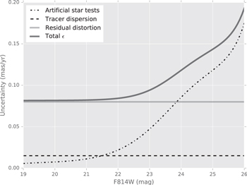
Figure 17. Run of adopted proper-motion uncertainty (per coordinate) against F814W apparent magnitude, including random uncertainty suggested by artificial-star tests (Calamida et al. 2015; dot-dashed line), the contribution due to intrinsic motion of the reference-frame tracer stars (dashed), and the estimated effect of residual differential distortion (gray solid line). Nearly all of our proper-motion sample falls in the range  (Figure 2). See the discussion in Appendix A.
Download figure:
Standard image High-resolution imageAppendix B: Gaussian Mixture Modeling
This work makes heavy use of a GMM to characterize overlapping populations in various spaces (e.g., Sections 3.3, 3.5, and 3.7). GMM is a standard technique in unsupervised machine learning (e.g., Bishop 2006), with growing use in astronomical data analysis (Ivezić et al. [2014] and Bovy et al. [2011] provide particularly clear and authoritative presentations of GMM in an astronomical context, including the extension of the methods to strongly nonuniform measurement uncertainty). Briefly, the sample is modeled as a sum of (k = 1...K) Gaussian components, with the mixture weight αk of each component (where  ) estimated by treating the unknown component identification of each object as a latent variable, fitting the mixture-model components θk iteratively along with the mixture weights, usually using the expectation-maximization algorithm or a variant thereof.
Under the GMM framework, we can write the formal membership probability  that a given object belongs to each model component (the "responsibility" in the language of Bishop 2006) as
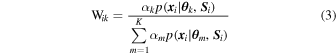
(as has been common practice for decades in the field of globular cluster studies, under slightly different notation). Here  represents the measured coordinates of the i'th object,
  the components of the k'th model in the mixture (i.e., its mean and covariance matrix), αk the relative weight of the k'th model component,
  the covariance matrix due to measurement uncertainty for the i'th object, and
  the likelihood of measuring
  given the k'th model parameters, assuming that the object does belong to that component.
B.1. Measurement Uncertainties in [t], [m]
From the definition of the ![$[t],[m]$](https://content.cld.iop.org/journals/0004-637X/858/1/46/revision1/apjaaba7fieqn272.gif) indices (Equation (1)), uncertainty propagation produces an approximation for the appropriate measurement uncertainty covariance
indices (Equation (1)), uncertainty propagation produces an approximation for the appropriate measurement uncertainty covariance  for each data point, which we reproduce here for convenience. We adopt
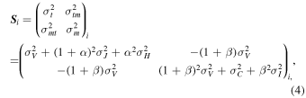
where  are the individual photometric uncertainty estimates in the BTS filters and (α, β) the appropriate scale factors for the indices (Equation (1)). Since α2 ≫ (1 + β) for these indices (for all populations of interest; Brown et al. 2009), we expect the covariance matrices for most of the stars to generally align with the
 ![$[t]$](https://content.cld.iop.org/journals/0004-637X/858/1/46/revision1/apjaaba7fieqn275.gif) direction, with only weak uncertainty covariance. Indeed, this is usually the case, though there are exceptions (Figure 18).
direction, with only weak uncertainty covariance. Indeed, this is usually the case, though there are exceptions (Figure 18).
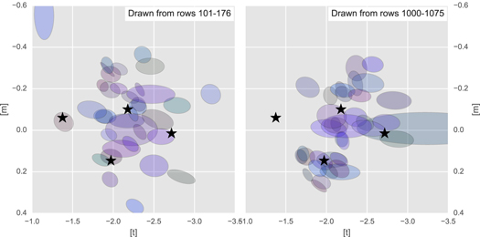
Figure 18. Covariance matrices  due to measurement uncertainty (following Equation (4)), for a randomly chosen selection of BTS measurements within the population selected for rotation curve study (Figure 2). Black stars show the central locations of the mixture-model components. Because both
 ![$[m]$](https://content.cld.iop.org/journals/0004-637X/858/1/46/revision1/apjaaba7fieqn277.gif) and
and ![$[t]$](https://content.cld.iop.org/journals/0004-637X/858/1/46/revision1/apjaaba7fieqn278.gif) contain F555W measurements, an appreciable tilt in the covariance matrices is often present. In many cases, the near-infrared measurements dominate the uncertainty, as expected given the large value of the scale factor α in the definition of
contain F555W measurements, an appreciable tilt in the covariance matrices is often present. In many cases, the near-infrared measurements dominate the uncertainty, as expected given the large value of the scale factor α in the definition of ![$[t]$](https://content.cld.iop.org/journals/0004-637X/858/1/46/revision1/apjaaba7fieqn279.gif) (Equation (1)). See the discussion in Appendix B.
(Equation (1)). See the discussion in Appendix B.
Download figure:
Standard image High-resolution imageWe are also assuming that the apparent magnitudes and their relevant linear combinations are normally distributed, working in apparent magnitude space rather than flux space because the photometric uncertainties are already reported in magnitudes in the BTS catalog. We impose a photometric uncertainty cut of σ < 0.1 mag (Table 3) to reduce the number of objects that strongly violate this assumption. Nevertheless, long tails in the observed ![$[t],[m]$](https://content.cld.iop.org/journals/0004-637X/858/1/46/revision1/apjaaba7fieqn280.gif) distribution for objects with relatively high photometric uncertainty may be expected.
distribution for objects with relatively high photometric uncertainty may be expected.
B.2. How Many Mixture Components?
To estimate the number of components required to best represent the ![$[t],[m]$](https://content.cld.iop.org/journals/0004-637X/858/1/46/revision1/apjaaba7fieqn281.gif) distribution, we employ two commonly used measures, the Akaike Information Criterion (AIC) and the Bayesian Information Criterion (BIC). These measures quantify the badness of fit while penalizing more complex models, with the BIC penalizing overly complex models more severely. More information can be found in Ivezić et al. (2014); these measures take the forms
distribution, we employ two commonly used measures, the Akaike Information Criterion (AIC) and the Bayesian Information Criterion (BIC). These measures quantify the badness of fit while penalizing more complex models, with the BIC penalizing overly complex models more severely. More information can be found in Ivezić et al. (2014); these measures take the forms


where lower values indicate a formally better fit. Here p is the number of parameters in the model, N the number of data points, and L the likelihood (data given model) returned by the mixture modeling procedure. For a GMM consisting of a mixture of K model components representing  -dimensional data points, the number of parameters p is given by

so that mixtures with K = 1, 2, 3, 4... model components consist of p = 5, 11, 17, 23... parameters when fitting the 2D ![$[t],[m]$](https://content.cld.iop.org/journals/0004-637X/858/1/46/revision1/apjaaba7fieqn283.gif) distribution. When characterizing the
distribution. When characterizing the ![$[m]$](https://content.cld.iop.org/journals/0004-637X/858/1/46/revision1/apjaaba7fieqn284.gif) or (
or (![$[t],[m]$](https://content.cld.iop.org/journals/0004-637X/858/1/46/revision1/apjaaba7fieqn285.gif) ) distribution with a GMM, we allow K to vary up to large values (usually K = 9) and look for models in which the AIC and BIC stop improving as K is increased.
) distribution with a GMM, we allow K to vary up to large values (usually K = 9) and look for models in which the AIC and BIC stop improving as K is increased.
Figure 19 shows an attempt to reproduce the distribution of ![$[m]$](https://content.cld.iop.org/journals/0004-637X/858/1/46/revision1/apjaaba7fieqn286.gif) only as a GMM (see Appendix B for discussion of the technique). At least two components seem to be required, although the data do not discriminate between the simplest model that fits the data (two components) and a continuum (e.g., eight components). In early trials using data selected only on photometric measurement uncertainty, a mixture model with more than three components would usually include an extremely broad, low-significance Gaussian component. On plotting the
only as a GMM (see Appendix B for discussion of the technique). At least two components seem to be required, although the data do not discriminate between the simplest model that fits the data (two components) and a continuum (e.g., eight components). In early trials using data selected only on photometric measurement uncertainty, a mixture model with more than three components would usually include an extremely broad, low-significance Gaussian component. On plotting the ![$[m]$](https://content.cld.iop.org/journals/0004-637X/858/1/46/revision1/apjaaba7fieqn287.gif) counts on a log scale, this component was seen to be fitting handfuls of far outliers in the
counts on a log scale, this component was seen to be fitting handfuls of far outliers in the ![$[m]$](https://content.cld.iop.org/journals/0004-637X/858/1/46/revision1/apjaaba7fieqn288.gif) distribution (with
distribution (with ![$| [m]| \gt 0.5;$](https://content.cld.iop.org/journals/0004-637X/858/1/46/revision1/apjaaba7fieqn289.gif) compare with the range in Figure 19). This may be expected if the outliers are not well represented by the model form; nevertheless, the GMM implementation would attempt to assign a model component to the outliers once the model grew sufficiently complex, which in turn would distort model components much nearer to the location of the main population of objects. Circumventing this outlier problem was the main motivator for outlier removal in
compare with the range in Figure 19). This may be expected if the outliers are not well represented by the model form; nevertheless, the GMM implementation would attempt to assign a model component to the outliers once the model grew sufficiently complex, which in turn would distort model components much nearer to the location of the main population of objects. Circumventing this outlier problem was the main motivator for outlier removal in ![$[t],[m]$](https://content.cld.iop.org/journals/0004-637X/858/1/46/revision1/apjaaba7fieqn290.gif) when selecting objects for further analysis (Table 3).
when selecting objects for further analysis (Table 3).
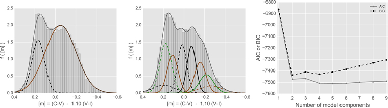
Figure 19. Left panel: distribution of ![$[m]$](https://content.cld.iop.org/journals/0004-637X/858/1/46/revision1/apjaaba7fieqn291.gif) , for objects satisfying −2.8 ≤
, for objects satisfying −2.8 ≤ ![$[t]$](https://content.cld.iop.org/journals/0004-637X/858/1/46/revision1/apjaaba7fieqn292.gif) ≤ −1.4, representing roughly the population within the outer contour in Figure 3. The gray shaded region shows the observed
≤ −1.4, representing roughly the population within the outer contour in Figure 3. The gray shaded region shows the observed ![$[m]$](https://content.cld.iop.org/journals/0004-637X/858/1/46/revision1/apjaaba7fieqn293.gif) distribution. The upper gray solid line shows a GMM trained on the
distribution. The upper gray solid line shows a GMM trained on the ![$[m]$](https://content.cld.iop.org/journals/0004-637X/858/1/46/revision1/apjaaba7fieqn294.gif) distribution. The colored solid and dashed curves show realizations of the individual model components. Middle panel: as in the left panel, but with an eight-component GMM specified as an ansatz for a continuum of populations. Right panel: formal assessment of the number of parameters required to reproduce the observed
distribution. The colored solid and dashed curves show realizations of the individual model components. Middle panel: as in the left panel, but with an eight-component GMM specified as an ansatz for a continuum of populations. Right panel: formal assessment of the number of parameters required to reproduce the observed ![$[m]$](https://content.cld.iop.org/journals/0004-637X/858/1/46/revision1/apjaaba7fieqn295.gif) distribution. Standard figures of merit, the BIC (black dashed line), and the AIC (gray solid line; see, e.g., Ivezić et al. 2014) are plotted as a function of the number of model components. A GMM representation of the
distribution. Standard figures of merit, the BIC (black dashed line), and the AIC (gray solid line; see, e.g., Ivezić et al. 2014) are plotted as a function of the number of model components. A GMM representation of the ![$[m]$](https://content.cld.iop.org/journals/0004-637X/858/1/46/revision1/apjaaba7fieqn296.gif) distribution seems to require at least two components, with little improvement for more complex models. See Appendix B.2.
distribution seems to require at least two components, with little improvement for more complex models. See Appendix B.2.
Download figure:
Standard image High-resolution imageFigure 20 shows the characterization of the (![$[t],[m]$](https://content.cld.iop.org/journals/0004-637X/858/1/46/revision1/apjaaba7fieqn297.gif) ) distribution with a 2D GMM as the number of model components is increased. To examine the impact of changing the number of model components K, the
) distribution with a 2D GMM as the number of model components is increased. To examine the impact of changing the number of model components K, the ![$[t],[m]$](https://content.cld.iop.org/journals/0004-637X/858/1/46/revision1/apjaaba7fieqn298.gif) data were split into two equal-size samples (the "training" and "test" sets), and the GMM fit using the "training" set. Samples (of
data were split into two equal-size samples (the "training" and "test" sets), and the GMM fit using the "training" set. Samples (of ![$[t],[m]$](https://content.cld.iop.org/journals/0004-637X/858/1/46/revision1/apjaaba7fieqn299.gif) ) were then drawn from the model and perturbed by measurement covariances
) were then drawn from the model and perturbed by measurement covariances  from the "test" set, and the (
![$[t],[m]$](https://content.cld.iop.org/journals/0004-637X/858/1/46/revision1/apjaaba7fieqn301.gif) ) distribution of this predicted set was compared with the "test" set. While models with K = 2, 3, 4 components each provide a reasonable visual match to the observed
) distribution of this predicted set was compared with the "test" set. While models with K = 2, 3, 4 components each provide a reasonable visual match to the observed ![$[t],[m]$](https://content.cld.iop.org/journals/0004-637X/858/1/46/revision1/apjaaba7fieqn302.gif) distribution, the AIC and BIC both indicate that K = 4 provides the best representation of the data, while increasing the number of components beyond K = 4 does not improve the fit further (indeed, the BIC suggests that models with K > 4 fit the data more poorly).
distribution, the AIC and BIC both indicate that K = 4 provides the best representation of the data, while increasing the number of components beyond K = 4 does not improve the fit further (indeed, the BIC suggests that models with K > 4 fit the data more poorly).
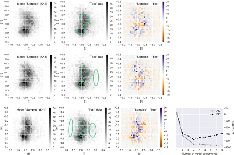
Figure 20. GMM of the population selected for rotation curve study. Reading top to bottom, panels show the GMM characterization for K = 2, 3, 4 mixture components. Left panels show the histogram of samples drawn from a GMM fit to a randomly selected sample of half the data (the "training set"). The middle left panels show the other half of the data (the "test set"), with the 1σ contours of the model components overplotted as thick cyan ellipses. The middle right panels show the residuals (samples from the model minus the observed counts in the "test set"). The bottom right panel shows formal fit statistics as a function of the number of model components. See Appendix B.2.
Download figure:
Standard image High-resolution imageAppendix C: Spectroscopic Estimate of the [Fe/H] Spread in SWEEPS-field Bulge Stars
An estimate of the spectroscopic metallicity distribution in this field is useful to calibrate synthetic stellar populations when investigating possible systematic effects. To perform this estimate, we use a deep set of VLT spectroscopic observations originally performed to provide radial velocity follow-up to the SWEEPS transiting planet candidates; details can be found in Sa06; here we outline the relevant features for the present paper.
C.1. Spectroscopic Observations of the SWEEPS Field
Fiber-fed echelle spectroscopy was taken using UVES between 2004 June 22 and 25 (ESO program 073.C-0410(A); PI Dante Minniti). [M/H] estimates were produced in a similar manner to the analysis in Fischer & Valenti (2005) and Valenti & Fischer (2005); typically ∼50 absorption features from a solar spectrum (numerically degraded to the spectral resolution of the observations) are scaled and shifted to find the best match to the observed spectra. In addition to radial velocities, this process also yielded estimates for [M/H] (as well as  and
and  ). The [M/H] determination used mainly metal lines, with very few C and O lines in the templates used, which reduces sensitivity in the [M/H] estimates to systematic differences between giants and MS objects (Valenti & Fischer 2005).
The 123 objects in the resulting catalog were trimmed by longitudinal proper motion (μl < −2.0 mas yr−1) to produce a sample of 93 likely bulge objects with spectroscopic [M/H] estimates.
C.2. GMM Characterization of the VLT Spectroscopic Sample
Following previous works, which use multicomponent Gaussian mixtures to model the [Fe/H] distributions (e.g., Hill et al. 2011; Schultheis et al. 2017; Zoccali et al. 2017), we also characterize the abundance distribution of the 93 spectroscopically measured likely bulge objects as a Gaussian mixture (Figure 21). Two implementations of GMM with uncertainties are used: the extreme-deconvolution method of Bovy et al. (2011), and scikit-learn XDGMM (Pedregosa et al. 2011). The parameters fitted by the two implementations are generally consistent with each other and are shown in Figure 21 and Table 9.
Figure 21. Left column: GMM decomposition of the 93 kinematically identified bulge objects with spectroscopic [Fe/H] estimates (Appendix C.1). Top left: visualization of a two-component GMM fit to the individual data points, over the histogram of the samples; middle and bottom left: two realizations of the GMM model. Solid lines refer to the model fit with the scikit-learn XDGMM implementation (Pedregosa et al. 2011), while dashed lines show the parameters fit using the extreme-deconvolution implementation of Bovy et al. (2011). The algorithm fits the underlying model distribution after correction for measurement uncertainty; the models and model samples have therefore been convolved with a Gaussian with the median measurement uncertainty for visualization. See Figure 21 and Appendix C. Right column: sample selection and mixture fit criteria for the characterization of the VLT spectroscopic abundance estimates (Appendix C.1). Top right: SWEEPS CMD showing all 123 spectroscopically sampled objects (black points) and the subset of 93 objects kinematically identified with the bulge (green squares). The bulge MS turnoff, giant branch, and disk MS are each apparent. Bottom right: the variation of formal figures of merit as a function of the number of model components. See Figure 21 and Appendix C.
Download figure:
Standard image High-resolution imageTable 9. GMM Fits to the SWEEPS Spectroscopic Sample of 93 Likely Bulge Objects
| k | αk (XD) | [Fe/H]0 (XD) | σ[Fe/H] (XD) | αk (ED) | [Fe/H]0 (ED) | σ[Fe/H] (ED) |
|---|---|---|---|---|---|---|
| 1 | 0.31 ± 0.049 | −0.42 ± 0.079 | 0.24 ± 0.059 | 0.26 ± 0.057 | −0.49 ± 0.056 | 0.16 ± 0.042 |
| 2 | 0.69 ± 0.049 | 0.24 ± 0.025 | 0.19 ± 0.020 | 0.74 ± 0.057 | 0.22 ± 0.027 | 0.19 ± 0.023 |
| 1 | 0.28 ± 0.046 | −0.48 ± 0.049 | 0.17 ± 0.041 | 0.28 ± 0.059 | −0.48 ± 0.061 | 0.17 ± 0.044 |
| 2 | 0.36 ± 0.086 | 0.13 ± 0.068 | 0.12 ± 0.062 | 0.27 ± 0.202 | 0.11 ± 0.110 | 0.11 ± 0.075 |
| 3 | 0.36 ± 0.086 | 0.34 ± 0.052 | 0.17 ± 0.039 | 0.45 ± 0.209 | 0.31 ± 0.176 | 0.18 ± 0.074 |
Note. Two GMM implementations are reported: "XD" refers to the scikit-learn XDGMM implementation, while "ED" refers to the extreme-deconvolution method of Bovy et al. (2011). Reported ranges denote the standard deviation over 500 nonparametric bootstrap resampling trials. Parameter sets are reported for two- and three-component mixture models.
Download table as: ASCIITypeset image
Although the 93 objects have somewhat limited statistical power to distinguish models, it does appear that at least a two-component mixture is preferred. At four or more components, both implementations always include a very broad, almost insignificant component, which suggests overfitting—and indeed the AIC and BIC do not suggest that more than two components are required by these data (Figure 21, right column).
The parameters of the two-component GMM are consistent with those reported by spectroscopic surveys of nearby fields (e.g., Schultheis et al. 2017; Zoccali et al. 2017), both of which find at least two spectroscopic components with similar fractions αk, centroids, and dispersions. The sample does not include a more metal-poor component that might be suggestive of a halo component (e.g., Ness et al. 2013a; Schultheis et al. 2017).
Appendix D: Differential Spread in Photometric Parallax
Since the distance determination is based on relative photometric parallax ( ), in principle the "metal-poor" population might be subject to additional photometric scatter that causes it to be more mixed in apparent distance than the "metal-rich" population (Section 5.1). Might differential distance blurring be responsible for the apparent differences in rotation curves, even if the intrinsic kinematic trends for both samples were identical?
To address this question, we perform simple Monte Carlo tests, communicated in this section. Differences in absolute magnitude distribution due to the differing stellar parameter ranges between the selected samples—particularly [Fe/H]—require a more sophisticated analysis and are discussed in Appendix E.
Individual objects in the "metal-rich" sample are perturbed in apparent magnitude, and the proper-motion rotation curve for the distance-blurred "metal-poor" sample is compared to the observed rotation curve for the "metal-poor" sample, by computing and comparing the smoothed rotation curves between distance moduli (−1.0 ≤  ≤ +1.0) for both samples.
For each form of distance modulus blurring, a run of 30 effect scales is considered. A thousand realizations were run at each of the effect scales, and the match between the distance-blurred "metal-rich" and the observed "metal-poor" rotation curves was evaluated. Three figures of merit are assessed: (i) The rms difference between the two trends is used as the primary badness-of-match statistic, where the longitudinal proper-motion offset between the two observed trends (+0.14 mas yr−1; Section 3.6) is subtracted from the "metal-rich" sample to ease interpretation (so that a perfect match between the two samples would produce badness-of-match value zero). In addition, the difference in  distribution between the blurred "metal-rich" and observed "metal-poor" samples is quantified by the difference in (ii) the
  standard deviations for each distribution and (iii) the skewness of the two
  distributions, since the observed "metal-poor" distance modulus distribution does exhibit an asymmetry toward the near side of the median population (e.g., Figures 6 and 7).
To determine the ranges of these figures of merit that would be consistent with a match, for every trial a control test is performed. A set of  values is drawn following the observed "metal-poor"
  distribution, and the observed "metal-poor" rotation curve (and proper-motion dispersion curve) is sampled at the generated
  values. For this generated sample, the rotation curve and comparison statistics are obtained exactly as for the blurred "metal-rich" sample. In this way, the figures of merit are also produced for a set of samples when the "metal-poor" distribution is compared against a statistical clone of itself, allowing the range of badness-of-fit values to be charted that suggest that the underlying samples are drawn from the same distribution.
Two forms of potential distance modulus blurring are considered independently. Additional scatter in the intrinsic flux distribution is discussed in Appendix D.1, which accounts for additional photometric uncertainty or differences in extinction (or indeed any perturbation that would lead to an additional flux perturbation of the same general form). The impact of differing binary fraction is discussed separately in Appendix D.2, because its imprint on the flux distribution takes a different form.
D.1. Additional Photometric Scatter in the "Metal-poor" Population
Additional photometric scatter is simulated as a perturbation in flux. The apparent magnitudes in the "metal-rich" sample are perturbed by amount Δmp, defined as

where ΔFi is the perturbation in flux, assumed normally distributed, s the scale of the additional flux uncertainty as a multiple of the original unperturbed flux F0,i, and  a draw from the unit normal distribution. For large values of s, the normally distributed flux perturbation can cause the perturbed flux values for some simulated objects to go negative; the simulation treats these cases as nondetections and removes affected objects from consideration, thus penalizing simulations with very large simulated flux uncertainty.
Figure 22 shows indications from this test. To aid interpretation in terms of apparent magnitude, we also characterize the sample standard deviation in apparent magnitude caused by the perturbation (which we denote  ), displaying it alongside the input scale s of flux perturbation; the quantity
  is plotted along the top axes in Figure 22. The rotation curve badness-of-match statistic suggests that observed rotation curve discrepancy can result from increased photometric scatter for scale factor s ≳ 0.35 (in apparent magnitude,
  ), while the
  distribution of the "metal-poor" sample is brought into rough agreement with that observed, for scale factor range
  (or in magnitudes,
  ).
).
Figure 22. Testing the hypothesis that additional flux scatter  can by itself cause identical rotation curves and
  distributions to exhibit the observed discrepancies between "metal-poor" and "metal-rich" samples. In each panel, the lower horizontal axes each show the scale s of the fractional flux perturbation, while the upper horizontal axes show
  , the corresponding sample standard deviation in apparent magnitude. Reading left to right, panels show the badness-of-match statistic, the difference in distance modulus standard deviations, and the difference in distance modulus skewness. Solid red lines show the median of each statistic, and 95% of the samples fall within the dashed contours. The blue shaded region and contours show the control test. See Appendix D.1.
Download figure:
Standard image High-resolution imageIt is difficult to see how the "metal-poor" sample might be subject to such a large additional photometric scatter. For example, the additional photometric scatter is likely far larger than the difference in photometric precision in the two samples from the SWEEPS measurements. Figure 23 shows the internal photometric precision (defined as the rms of the apparent magnitude measurements along the set of images) as a function of apparent magnitude and  for objects in the "metal-rich" and "metal-poor" samples. The "metal-poor" population shows only a slight increase in internal photometric uncertainty compared to the "metal-rich" population, and both are very small (on the order of a few mmag; these objects are well above the photometric completeness limit for the SWEEPS survey). While indeed the internal precision refers to the random component of photometric uncertainty and not the absolute photometric accuracy, a sample difference in photometric uncertainty of ∼0.3–0.5 mag seems highly unlikely for these data.
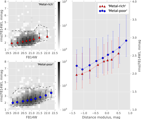
Figure 23. Comparison of internal photometric precision for the "metal-rich" and "metal-poor" samples as a function of apparent magnitude (left) and distance modulus (right). Error bars indicate the upper and lower bounds within which 68% of objects are found in each bin, the dashed contours encompass 95% of objects per bin, and the plot symbols show the medians. The gray scale shows object counts in the two samples, on a logarithmic scale. See Appendix D.1.
Download figure:
Standard image High-resolution imageA difference in extinction distribution between the samples, characterized in any way,31
if large enough to bring about the  ∼ 0.3–0.5 mag additional scatter required, would surely have led to additional observational consequences that are not seen in these data. For example, the observed F814W dispersion of the RCGs in the SWEEPS data set is close to
  mag (Cl08). Even if all this dispersion were due to extinction, which seems unlikely, this would still be a factor ≳2 too low to bring about the observed discrepancies between "metal-rich" and "metal-poor" samples.
When the depth of the bulge along the line of sight is considered, the allowed contribution of differential extinction to  blurring becomes somewhat smaller. For example, assuming that the bulge RCGs are scattered along this line of sight by ±0.50 kpc allows room for only 0.1 mag of photometric blurring due to extinction of any prescription. Since extinction effects would need to apply differentially to the "metal-poor" sample compared to the "metal-rich" sample to bring the two rotation curves into agreement, we conclude that differential extinction effects are likely at least a factor of 3–5 too small to account for the observed rotation curve discrepancy.
It is also not clear why the "metal-poor" sample would be subject to a strongly discrepant extinction distribution (however parameterized) in the first place. The two populations are not strongly different in their projected distributions on the sky (Figure 24), which would seem to argue against, say, the "metal-poor" sample being located within a region on the sky showing stronger, clumpier extinction than the "metal-rich" sample. Additionally, the RCG apparent magnitude distribution in this field does not appear to be bimodal (e.g., Clarkson et al. 2011; Nataf et al. 2013).
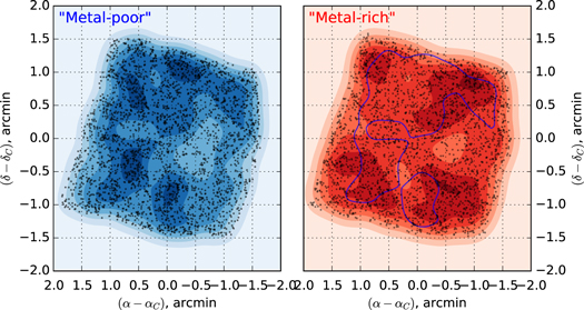
Figure 24. Spatial distributions of the "metal-poor" (blue, left) and "metal-rich" (red, right) populations discussed in Section 3.5, over the ∼3' × 3' of the BTS-SWEEPS cross-matched field. In each panel, points represent the individual objects, while the filled contours indicate the KDE representation of the local density at each point. In both panels, contours correspond to six equally spaced density levels. To aid visual comparison, the outer contour of the second-highest level from the metal-poor population is plotted over the metal-rich distribution in the right panel. See Appendix D.1.
Download figure:
Standard image High-resolution imageWe point out that this test applies to the dispersion of differential extinction, not to differences in the median extinction between the two samples. Although a difference in median RV might affect the drawing of the "metal-rich" and "metal-poor" samples using ![$[m]$](https://content.cld.iop.org/journals/0004-637X/858/1/46/revision1/apjaaba7fieqn328.gif) ,
, ![$[t]$](https://content.cld.iop.org/journals/0004-637X/858/1/46/revision1/apjaaba7fieqn329.gif) (because those indices are computed in terms of extinction ratios, which are dependent on the prescription for extinction), it would not by itself change the
(because those indices are computed in terms of extinction ratios, which are dependent on the prescription for extinction), it would not by itself change the  dispersion for a given population (RV variations are considered in more detail in Appendix E.5). The
  values for "metal-rich" and "metal-poor" populations are both constructed by reference to fiducial ridgelines fit to the observed populations in the SWEEPS CMD. While the interpretation of a given ridgeline with a particular set of population parameters (like [Fe/H],
  ,
,  ,
,  , and, to a lesser extent for this population, age) does depend on the median
  , this does not impact the fiducial ridgelines of the observed median populations on the SWEEPS CMD.
We thus reject additional photometric scatter as a cause for the "metal-rich" and the "metal-poor" samples to be drawn from the same kinematic population, because, whatever the cause, its likely magnitude is much too low to have gone unnoticed elsewhere in these data.
D.2. Differences in Binary Fraction
If the "metal-poor" sample has a highly discrepant binary fraction or binary companion mass ratio distribution from the "metal-rich" sample, then this might produce a population with larger distance spread, where the additional inferred distance scatter would be biased to closer distances than the mean population—qualitatively similar to the trends observed (e.g., Figure 7).
The binary fraction  , minimum binary (initial) mass ratio
  , and indeed the shape of the distribution of mass ratio q are not known for the bulge (see, e.g., Calamida et al. 2015) and are difficult to constrain observationally for the sample selected for the present proper-motion study (e.g., Figure 2). A complete search of (
 ,
,  ) parameter space, and indeed of the form of the mass ratio distribution, is beyond the scope of the present investigation. Instead, we characterize statistically the distribution of
  due to unresolved binaries, for the CMD region of interest to this study (Figure 2), and draw from this distribution
  for each realization of the Monte Carlo trial.
To maximize the impact of a difference in binary fraction between the "metal-rich" and "metal-poor" samples, we assume for the purposes of this test that the "metal-rich" population has no binaries at all, and we perturb it using an unresolved binary fraction to approximate the "metal-poor" population. (This thus allows the excess binary fraction to be tested in the range 0 ≤  ≤ 1; if we assume that the "metal-rich" sample has a binary fraction of 0.3, then only tests in the range
  < 0.7 would be meaningful.) We also assume for this test that it is only the population of unresolved binaries that differs between the two samples (i.e., there is no difference in metallicity distribution between the two samples).
Version 5.0.1 of the BaSTI 32
suite of simulation tools and stellar population models (Pietrinferni et al. 2004, 2006) is used to produce a representative set of distributions  , to characterize for the Monte Carlo draws. Thanks to the capability of BaSTI to accept user-defined random number seeds, simulations that are almost identical except for small changes in input parameters can be run. This allows us to compare synthetic populations on a star-by-star basis, with and without the addition of unresolved binaries.33
To combine the sophistication of BaSTI with the speed necessary for Monte Carlo trials, the distribution  itself is characterized nonparametrically, using the method outlined in Ivezić et al. (2014, their Section 3.7)—and thus does not depend on a functional form for
  . This resampling is 105–6 times faster than running a BaSTI simulation for each iteration and brings into reach Monte Carlo exploration of the impact of binaries for our purposes here.
BaSTI simulations are run for four choices of the minimum binary initial mass ratio:  = (0.0, 0.3, 0.5, 0.7). The "bulge" star formation history (Mollá et al. 2000) within BaSTI is used to populate the sample, with scaled-to-solar heavy-element abundances and the Kroupa et al. (1993) initial mass function. Absolute magnitudes are converted to apparent magnitudes using a fiducial distance and reddening. This allows
  to be characterized specifically for the population we have selected for proper-motion study. For
  = 0.0, the distribution
  turns out to closely resemble
  = 1/
= 1/ , while for
  > 0 the distribution becomes more complicated and nonparametric resampling is preferred (Figure 25).
Figure 25. Characterization of the distribution of apparent magnitude perturbation due to unresolved binaries, using the BaSTI suite of models and stellar population tools. Bottom left: synthetic stellar populations in the SWEEPS filter set. Red points show the simulation without binaries, gray the population with binaries. Faint points show a representative set of the entire simulation in each case; dark points show the objects that fall within the CMD selection region in the presence of unresolved binaries. Top left:  due to the presence of unresolved binaries, for objects only within the selection region. Top right: distribution of
  (on a log scale), with histogram boundaries at the upper end of each bin. This panel includes objects not assigned a binary companion in the simulation. Bottom right: normalized distribution of
  for objects assigned a binary companion (gray shading). The green open histogram shows the distribution of draws from a nonparametric resampling of
  . See Appendix D.2.
Download figure:
Standard image High-resolution imageIn none of the cases ( = 0.0, 0.3, 0.5, 0.7) do we find that the presence of an additional binary population can account for the difference between the observed "metal-rich" and "metal-poor" rotation curves. (Figure 26 shows the cases
  = 0.0 and
  = 0.7). Only the skewness of the
  distribution ever approximates that of the "metal-poor" population (at
  ≳ 0.5), while the rotation curve and
  spread do not overlap for any binary fraction.
Figure 26. Evaluation of the impact of a difference in binary fraction between "metal-rich" and "metal-poor" populations, in this case for q ≥ 0 (top row) and q ≥ 0.7 (bottom row). Panels, colors, and symbols are as in Figure 22; here, the binary fraction  is varied between trials. As with Figure 22, 95% of the samples fall within the dashed contours. See Appendix D.2
Download figure:
Standard image High-resolution imageWe therefore conclude that an excess of unresolved binaries in the "metal-poor" over the "metal-rich" population is highly unlikely to be responsible for the difference in rotation curves.
Appendix E: The Impact of Differential [Fe/H] Dispersion on Photometric Parallax
Under a model in which the bulge contains at least two metallicity components, with differing [Fe/H] dispersions, the spread in inferred photometric parallax within identified "metal-poor" and "metal-rich" samples will also differ, even if there is no difference in intrinsic distance distribution along the line of sight. Here we examine the likely magnitude of this systematic.
The method is outlined in Appendix E.1, with simulated population components described in Appendix E.2. In the course of this investigation, it became apparent that the widely used BaSTI simulation framework truncates samples at [Fe/H] values well within the limits of likely values in the SWEEPS field; the technique used to characterize absolute magnitude spread in the presence of this truncation is described in Appendix E.3. Finally, the differential scatter between "metal-rich" and "metal-poor" populations is presented in Appendix E.4. (The BaSTI truncation itself is characterized in Appendix F.)
E.1. General Method
To estimate the differential scatter in photometric parallax produced by differing [Fe/H] dispersions between "metal-rich" and "metal-poor" samples, a synthetic composite stellar population is produced for the SWEEPS field by sampling BaSTI simulations (computed for all three cameras and resampled in the manner of Appendix D.2), which include the effects of age, [Fe/H] spread, and unresolved stellar binaries. The synthetic populations are perturbed by photometric uncertainty (in all seven filters), photometric parallax, and reddening, where the width of the distributions in all three quantities can be specified separately for each population.
This produces a SWEEPS CMD and ![$[t],[m]$](https://content.cld.iop.org/journals/0004-637X/858/1/46/revision1/apjaaba7fieqn365.gif) distribution for the synthetic population. Synthetic objects are selected for further "study" in a similar manner to that for the real data (e.g., Table 3); in particular, synthetic SWEEPS CMD objects must fall within the selection box in the SWEEPS filters (Figure 2). The surviving synthetic objects are then classified as likely "metal-poor" and "metal-rich" populations in the same manner as for the observed data (using the GMM components in
distribution for the synthetic population. Synthetic objects are selected for further "study" in a similar manner to that for the real data (e.g., Table 3); in particular, synthetic SWEEPS CMD objects must fall within the selection box in the SWEEPS filters (Figure 2). The surviving synthetic objects are then classified as likely "metal-poor" and "metal-rich" populations in the same manner as for the observed data (using the GMM components in ![$[t],[m]$](https://content.cld.iop.org/journals/0004-637X/858/1/46/revision1/apjaaba7fieqn366.gif) that were fitted to the real data), isolating "observed" samples of "metal-rich" and "metal-poor" objects. In this manner, the synthetic samples are isolated in a similar fashion to those drawn from the real data.
that were fitted to the real data), isolating "observed" samples of "metal-rich" and "metal-poor" objects. In this manner, the synthetic samples are isolated in a similar fashion to those drawn from the real data.
Finally, best-fit loci are determined for the model absolute magnitudes of the synthetic "metal-rich" and "metal-poor" samples, and the differences ΔMV from these loci are determined for every object in the samples. The model absolute magnitude is used rather than the apparent magnitude because we wish to isolate the impact of metallicity spread on intrinsic magnitude scatter—i.e., before distance, reddening, and photometric uncertainty have perturbed the measurements (which impacts the sample selection), but including the intrinsic effects of age, [Fe/H], and binarity.
Modeling the selection cuts on the synthetic samples requires simulating the composite stellar population of the SWEEPS field. This field is somewhat complex, consisting of at least three distinct populations (bulge, local disk, halo), each of which could well consist of multiple subpopulations or a continuum.
Full population decomposition presents a formidable challenge (e.g., Gennaro et al. 2015) and is complicated by the difficulty in adequately accounting for extinction across the broad wavelength range of the BTS photometry in the inner bulge region (e.g., Nataf et al. 2016). To produce a reasonable approximation to the selection effects at work in the SWEEPS field, a multicomponent stellar population is instead simulated with parameters drawn from the literature and the [Fe/H] spread estimated in this work (Appendix C). A set of about a dozen synthetic populations with various parameter settings are simulated using BaSTI, with typically five components from this set combined appropriately to produce a synthetic composite population for the SWEEPS field, with mixture parameters tuned by hand to provide an approximate match to the observed SWEEPS CMD and ![$[t],[m]$](https://content.cld.iop.org/journals/0004-637X/858/1/46/revision1/apjaaba7fieqn367.gif) distribution.
distribution.
E.2. Synthetic Population Components
All population components used the same prescription for binaries, with binary fraction 0.35 and minimum binary mass ratio 0.0. The initial mass function followed the Kroupa et al. (1993) prescription for all components over the BaSTI default mass range ( ). Convective core overshooting was not selected for any model component, and mass-loss parameter η = 0.4 was used throughout. When not using a predetermined star formation history supplied by BaSTI, the star formation histories were specified as a series of single bursts at given ages, with [Fe/H] described as a Gaussian with a user-specified centroid and standard deviation. Specific details for various population components follow below.
For the foreground disk, the formation history of Rocha-Pinto et al. (2000) was used (the default "local disk" scenario within BaSTI), typically forming 5%–10% of the stars in the simulation sets.
Stellar halo components were simulated using the bimodal [Fe/H] distribution reported by An et al. (2013) from Sloan Digital Sky Survey photometry; this model consists of a very metal-poor component centered at [Fe/H] ≈ −2.33 and another slightly less metal-poor component centered at [Fe/H] ≈ −1.67. For a bimodal bulge population following any of the GMM fits to our spectroscopic data, or for the [Fe/H] distribution of Zoccali et al. (2017) near the SWEEPS field, this separate halo component is necessary to populate the regions in ![$[t],[m]$](https://content.cld.iop.org/journals/0004-637X/858/1/46/revision1/apjaaba7fieqn369.gif) space for objects with [Fe/H] ≲ −2.0.
space for objects with [Fe/H] ≲ −2.0.
Bulge components were constructed separately as normally distributed [Fe/H] distributions specified through the BaSTI web interface, using the characterization presented in Appendix C, for both the two- and three-component GMM decompositions. For components less metal-rich than [Fe/H]0 < + 0.3, separate runs were simulated using the "scaled-to-solar" and "α-enhanced" options within BaSTI in order to allow some exploration of α-enhancement on population spread in the ![$[t],[m]$](https://content.cld.iop.org/journals/0004-637X/858/1/46/revision1/apjaaba7fieqn370.gif) diagram. A variety of age prescriptions were attempted, mostly to improve the match at the bright end of the SWEEPS CMD, either by ascribing a single burst of star formation to each metallicity or by assigning several bursts to each metallicity (e.g., bursts at 5.0, 6.0, and 7.0 Gyr for a component with [Fe/H]0 = −0.42). We have not yet explored more sophisticated age–metallicity prescriptions through user-defined star formation histories (e.g., Haywood et al. 2016; Bensby et al. 2017).
diagram. A variety of age prescriptions were attempted, mostly to improve the match at the bright end of the SWEEPS CMD, either by ascribing a single burst of star formation to each metallicity or by assigning several bursts to each metallicity (e.g., bursts at 5.0, 6.0, and 7.0 Gyr for a component with [Fe/H]0 = −0.42). We have not yet explored more sophisticated age–metallicity prescriptions through user-defined star formation histories (e.g., Haywood et al. 2016; Bensby et al. 2017).
The more continuous bulge star formation history of Mollá et al. (2000, used as a default in BaSTI) was also tried, for "scaled-to-solar" isochrones, for "α-enhanced" isochrones, and for varying admixtures of the two.
We have not yet explored a separate "thick-disk" component in this context. The metal-poor wing of the bulge distribution or the metal-rich wing of the halo component could mimic such a population in the ![$[t],[m]$](https://content.cld.iop.org/journals/0004-637X/858/1/46/revision1/apjaaba7fieqn371.gif) diagram, and we do not make the distinction here.
diagram, and we do not make the distinction here.
Figures 27 and 28 show examples of the synthetic populations thus produced. None of the population mixtures that we have produced quite reproduce both the observed SWEEPS CMD and the ![$[t],[m]$](https://content.cld.iop.org/journals/0004-637X/858/1/46/revision1/apjaaba7fieqn372.gif) diagram, although in view of both the challenges of extinction characterization and apparent simulation truncations imposed by BaSTI itself (Appendix E.3), full reproduction is likely to be difficult. The basic two-component bulge we simulate here produces an
diagram, although in view of both the challenges of extinction characterization and apparent simulation truncations imposed by BaSTI itself (Appendix E.3), full reproduction is likely to be difficult. The basic two-component bulge we simulate here produces an ![$[t],[m]$](https://content.cld.iop.org/journals/0004-637X/858/1/46/revision1/apjaaba7fieqn373.gif) distribution that is much more strongly bimodal than that observed (e.g., Figure 3), while the 10-component "bulge" star formation history within BaSTI (Mollá et al. 2000) produces an
distribution that is much more strongly bimodal than that observed (e.g., Figure 3), while the 10-component "bulge" star formation history within BaSTI (Mollá et al. 2000) produces an ![$[t],[m]$](https://content.cld.iop.org/journals/0004-637X/858/1/46/revision1/apjaaba7fieqn374.gif) distribution that is too smooth compared to that observed.
distribution that is too smooth compared to that observed.
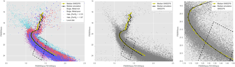
Figure 27. Composite simulated SWEEPS population. Left panel: synthetic populations. Red and blue circles show metal-rich and metal-poor bulge components, respectively, violet and gray triangles show the halo components, and cyan squares show the local disk populations. Middle and right panels: observed SWEEPS CMD, with the median simulated (black line and squares in all three panels) and SWEEPS (yellow line and circles in all three panels) populations. See Appendix E.2 for details.
Download figure:
Standard image High-resolution imageSeveral methods were attempted to bring the simulated ![$[t],[m]$](https://content.cld.iop.org/journals/0004-637X/858/1/46/revision1/apjaaba7fieqn375.gif) distribution into closer agreement with that of the observed data in Figure 3. One simple ansatz is to simply multiply the BTS estimated photometric uncertainties by a factor of 2 before selection and computation of
distribution into closer agreement with that of the observed data in Figure 3. One simple ansatz is to simply multiply the BTS estimated photometric uncertainties by a factor of 2 before selection and computation of ![$[t],[m]$](https://content.cld.iop.org/journals/0004-637X/858/1/46/revision1/apjaaba7fieqn376.gif) (Figure 28, top right panel). Another is to apply Gaussian blurring in
(Figure 28, top right panel). Another is to apply Gaussian blurring in ![$[t]$](https://content.cld.iop.org/journals/0004-637X/858/1/46/revision1/apjaaba7fieqn377.gif) and
and ![$[m]$](https://content.cld.iop.org/journals/0004-637X/858/1/46/revision1/apjaaba7fieqn378.gif) separately (bottom middle panel of Figure 28). Varying RV with a Gaussian of width
separately (bottom middle panel of Figure 28). Varying RV with a Gaussian of width  does bring the marginal distribution reasonably close to that observed (bottom right panel of Figure 28), although the
 ![$[t],[m]$](https://content.cld.iop.org/journals/0004-637X/858/1/46/revision1/apjaaba7fieqn380.gif) distribution that results is distorted compared to the observed sample (particularly the "metal-rich" sample), and in addition the required
distribution that results is distorted compared to the observed sample (particularly the "metal-rich" sample), and in addition the required  is at least a factor of ∼2 larger than that suggested by the SWEEPS CMD (Appendix E.5, which also shows the
 ![$[t],[m]$](https://content.cld.iop.org/journals/0004-637X/858/1/46/revision1/apjaaba7fieqn382.gif) -blurring effect due to RV variations that are compatible with the SWEEPS data).
-blurring effect due to RV variations that are compatible with the SWEEPS data).
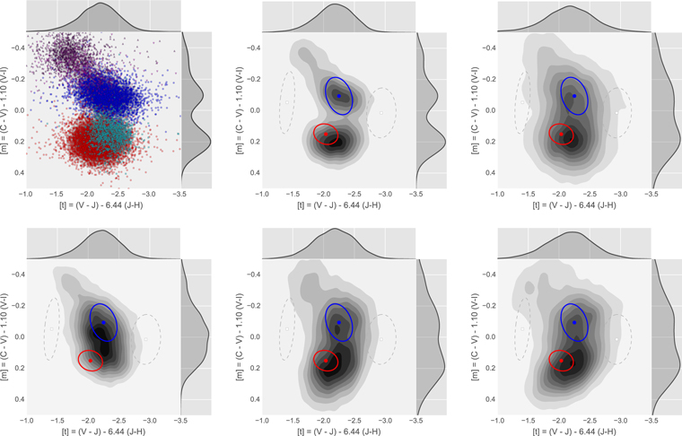
Figure 28. Example synthetic populations used to estimate metallicity effects on sample selection and measured relative photometric parallax distributions; all panels show the ![$[t],[m]$](https://content.cld.iop.org/journals/0004-637X/858/1/46/revision1/apjaaba7fieqn383.gif) distributions of the model populations with marginal distributions of
distributions of the model populations with marginal distributions of ![$[t]$](https://content.cld.iop.org/journals/0004-637X/858/1/46/revision1/apjaaba7fieqn384.gif) and
and ![$[m]$](https://content.cld.iop.org/journals/0004-637X/858/1/46/revision1/apjaaba7fieqn385.gif) plotted over the top and right axes, respectively (compare with Figure 3). All but the bottom left panel show populations with the same intrinsic parameters, modified observationally in different ways. Top left: example
plotted over the top and right axes, respectively (compare with Figure 3). All but the bottom left panel show populations with the same intrinsic parameters, modified observationally in different ways. Top left: example ![$[t],[m]$](https://content.cld.iop.org/journals/0004-637X/858/1/46/revision1/apjaaba7fieqn386.gif) distribution; symbols label components of origin in the same way as in Figure 27. Top middle: KDE representation of the simulation in the top left panel, with the "metal-rich" and "metal-poor" model components that were fitted to the observed data overlaid as ellipses for reference. Top right: population parameters as with the top middle panel, but with photometric uncertainties in the BTS filters multiplied by a factor of 2 to enhance scatter. Bottom left: bulge components drawn from BaSTI's "bulge" star formation history (Mollá et al. 2000), using one set each with BaSTI's α-enhanced and scaled-to-solar isochrone sets. Bottom middle: population parameters as for the top middle panel, but with
distribution; symbols label components of origin in the same way as in Figure 27. Top middle: KDE representation of the simulation in the top left panel, with the "metal-rich" and "metal-poor" model components that were fitted to the observed data overlaid as ellipses for reference. Top right: population parameters as with the top middle panel, but with photometric uncertainties in the BTS filters multiplied by a factor of 2 to enhance scatter. Bottom left: bulge components drawn from BaSTI's "bulge" star formation history (Mollá et al. 2000), using one set each with BaSTI's α-enhanced and scaled-to-solar isochrone sets. Bottom middle: population parameters as for the top middle panel, but with ![$[t],[m]$](https://content.cld.iop.org/journals/0004-637X/858/1/46/revision1/apjaaba7fieqn387.gif) each blurred by independent Gaussians, with width parameter σ[t] = 0.15 and σ[m] = 0.05. Bottom right: population parameters as per the top-middle panel, but with RV normally distributed at RV = 2.5 ± 0.52 in order to bring the marginal distributions roughly into line with those observed. See Appendix E.2 for details.
each blurred by independent Gaussians, with width parameter σ[t] = 0.15 and σ[m] = 0.05. Bottom right: population parameters as per the top-middle panel, but with RV normally distributed at RV = 2.5 ± 0.52 in order to bring the marginal distributions roughly into line with those observed. See Appendix E.2 for details.
Download figure:
Standard image High-resolution imageFor the purposes of estimating the impact of varying [Fe/H] distribution on relative photometric parallax variations, we retain the two-component bulge model with and without BTS uncertainty scaling, for further investigation; the former is consistent with estimated [Fe/H] distributions and estimates of photometric uncertainty, while the latter is the "broadened" option among those tried that closely resembles the observed distribution (Figure 3).
E.3. Characterizing Excess Variability in the Presence of Truncation
While conducting tests on the simulated data sets, it quickly became apparent that samples generated with the current version of BaSTI34 show truncation at extremes of both high and low metallicity, leading to a hard edge in the CMD of the simulated population that has no counterpart in the reported [Fe/H] distribution. This truncation, characterized in Appendix F, impacts the metal-rich simulated bulge sample more strongly than its metal-poor simulated counterpart and thus could artificially enhance the discrepancy in absolute magnitude breadth between the metal-rich and metal-poor simulated components.
This hidden systematic complicates efforts to characterize the excess magnitude scatter due to differing [Fe/H] distributions, with much of the most metal-rich end of the metal-rich simulated sample assigned apparently incorrect magnitudes (absolute and apparent). We therefore adopt a restricted-sample estimate of the magnitude scatter, by sampling only the fainter side of the magnitude distribution for both samples in the comparison. Specifically, we use the quantity σhi defined by35

where, for the special case of a large, strictly symmetric distribution, σhi closely approximates the sample standard deviation. A practical challenge is to identify the median magnitude  from a truncated asymmetric distribution. For these simulations,
  is estimated by discarding the most negative Δm samples (thus discarding objects near and outside the truncation limits) and fitting a Gaussian function to the histogram of Δm values. This fit is only used to estimate
  , which thus allows σhi to be estimated following Equation (9). This then allows the restricted-sample scatter σhi to be estimated for the metal-poor and metal-rich samples separately, and the excess difference to be characterized as the quadrature difference between the two.
The final step is then to convert the excess scatter  estimated from the simulated population components to the additional flux scatter s felt by the metal-poor sample compared to the metal-rich sample. To enable this conversion, the relationship between restricted-sample scatter σhi and the flux perturbation scale s that generated it was determined by simulation. Synthetic populations with perturbation flux distribution were produced following Equation (8), subject to the same censoring for negative flux as before (Appendix D.1). The apparent magnitude scatter σhi was then found for each synthetic population as described above (and as performed for the simulated BaSTI data sets). Finally, the relationship between
  and s was characterized by fitting a seventh-order polynomial in both directions. Table 10 and Figure 29 show this characterization. This allows us to relate the restricted-sample scatter found from BaSTI simulations back to the flux ratio perturbation scale s, and finally to compare the scale of the perturbation suggested by differing [Fe/H] distributions to the additional scale of flux perturbations s that our observational data would require if the "metal-poor" sample really were a blurred version of the "metal-rich" sample.
Figure 29. Charting the relationship between the flux standard deviation s (Appendix D.1) and the apparent magnitude scatter σhi for truncated samples (Equation (9)). Simulated perturbed populations are generated following Equation (8), and the absolute magnitude distribution of the resulting sample is characterized by σhi. Standard uncertainty propagation predicts s ≈ σ/1.086 (with σ the apparent magnitude standard deviation); in practice, we fit functional forms to transform between s and σhi. The top panel shows s and σhi along with the functional forms in both directions (seventh-order polynomials in log10-space). The bottom panel shows fractional residuals when σhi is used to predict s (residuals in the reverse direction are not shown); the polynomial approximation f7 is accurate to better than 2% over most of the range of interest. See Appendix E.3 and Table 10.
Download figure:
Standard image High-resolution imageTable 10. Polynomial Coefficients Relating the Flux Spread s (Appendix D.1) to Apparent Magnitude Scatter σhi (Equation (9)), over the Domain 0.01 ≤ σhi ≤ 1.0
| Coeff | i = 7 | 6 | 5 | 4 | 3 | 2 | 1 | 0 |
|---|---|---|---|---|---|---|---|---|
| ai | 0.2621 | 1.9750 | 6.0299 | 9.5353 | 8.1928 | 3.4773 | 1.2929 | −0.2817 |
| bi | 0.6190 | 4.3495 | 11.7411 | 14.7695 | 7.7084 | 0.0234 | 0.1323 | 0.1298 |
Note. The forms used are  and
and  . See Figure 29 and Appendix E.3.
Download table as: ASCIITypeset image
E.4. Differential Photometric Parallax Dispersion Due to Differential [Fe/H] Dispersion
We are finally in a position to estimate the additional scatter in absolute magnitude due to differential metallicity scatter. Figure 30 shows the results of applying the selection criteria to the simulation including the two-component bulge model, a two-component halo, and the local disk component.
Figure 30. Estimating the ridgelines for simulated objects that would be selected in the "metal-poor" (left panel) or "metal-rich" (right panel) samples. In each case absolute magnitudes are plotted in the SWEEPS filters. The component of origin for each simulated object surviving selection criteria is indicated by color and plotting symbol. See Appendix E.4.
Download figure:
Standard image High-resolution imageFigure 31 illustrates the characterization of absolute magnitude scatter σhi, while Table 11 shows the evaluation of the excess flux scatter s for "metal-poor" compared to "metal-rich" samples. Two simulated populations were evaluated in this manner: one including the two-component bulge model, and the other with the BTS uncertainties multiplied by a factor of 2 before selection to broaden the distribution in ![$[t],[m]$](https://content.cld.iop.org/journals/0004-637X/858/1/46/revision1/apjaaba7fieqn398.gif) . In both cases, the excess fractional flux scatter s is less than 0.1; we find s ≈ 0.09 for the two-component bulge model, while s ≈ 0.07 for the enhanced-uncertainty version of this model.
. In both cases, the excess fractional flux scatter s is less than 0.1; we find s ≈ 0.09 for the two-component bulge model, while s ≈ 0.07 for the enhanced-uncertainty version of this model.
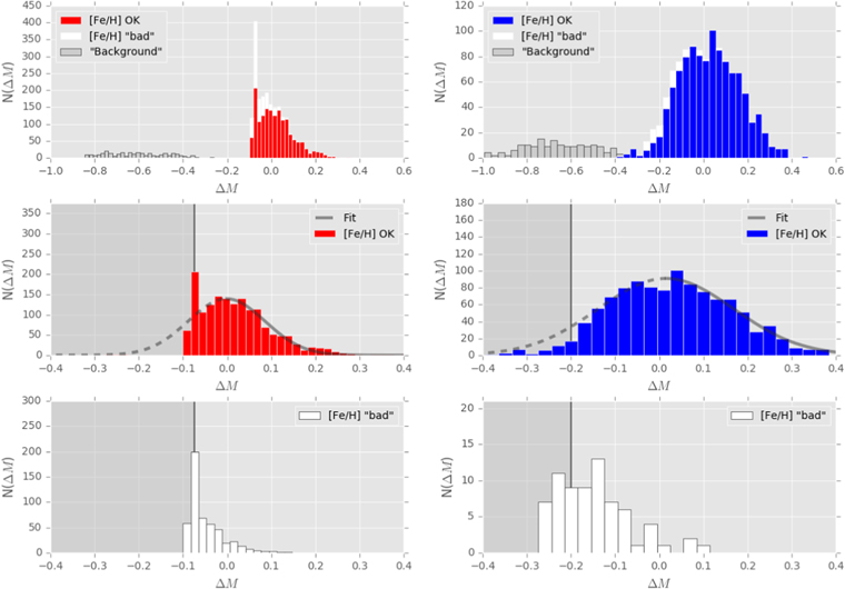
Figure 31. Characterizing the magnitude scatter σhi (Equation (9)) for simulated populations in the presence of truncation. The left column shows the simulated metal-rich population, the right column the simulated metal-poor population. White shaded bars in each figure show objects with [Fe/H] outside the adopted BaSTI metallicity range (using scaled-to-solar isochrones for the metal-rich column and α-enhanced isochrones for the metal-poor column). Rows show the full distribution (top), objects with simulated [Fe/H] within the nominal ranges (middle), and those outside the nominal ranges (bottom). The gray regions in the middle and bottom rows (delimited by the solid vertical line) show regions of ΔM excluded from the Gaussian fits to the distributions (smooth lines). The fitted median of ΔM is marked by a transition from solid to dashed line in the curves. Before characterization, each simulated sample is divided into a dominant and secondary component; the secondary component, mostly made up of unresolved binaries and labeled "Background" in the panels here, is excluded from further consideration. Note that (i) both the metal-rich and metal-poor samples include objects with reported [Fe/H] above the adopted upper limit; (ii) the truncation appears to impact objects even with [Fe/H] nominally within the adopted [Fe/H] limits, particularly for the metal-rich simulated population; and (iii) the strong truncation in the metal-rich sample leads to a large gap between the dominant and secondary components. See Appendix E.4.
Download figure:
Standard image High-resolution imageTable 11. Characterization of the Additional Absolute Magnitude Scatter Due to [Fe/H] for Simulated Metal-rich and Metal-poor Populations
| Component | σhi | s | σhi(broadened) | s(broadened) |
|---|---|---|---|---|
| Metal-poor | 0.137 | 0.112 | 0.153 | 0.124 |
| Metal-rich | 0.103 | 0.087 | 0.119 | 0.099 |
| Excess | 0.090 | 0.071 | 0.097 | 0.075 |
Note. The quadrature difference between the two samples is reported in the final line. σhi reports an estimate of the asymmetrically sampled absolute magnitude scatter (Appendix E.3), while s reports the scatter in the flux perturbation due to [Fe/H] spread. The first column pair shows results for the simulated populations and estimated uncertainties; the final column pair shows results for ![$[t],[m]$](https://content.cld.iop.org/journals/0004-637X/858/1/46/revision1/apjaaba7fieqn399.gif) distribution broadened to more accurately match the observed distribution. See Appendix E.4.
distribution broadened to more accurately match the observed distribution. See Appendix E.4.
Download table as: ASCIITypeset image
We contacted the authors of the BaSTI web tools regarding its internal truncation (detailed in Appendix F). In response, S. Cassisi (2017, private communication) kindly added a high-metallicity point to BaSTI's internal metallicity grid (since in BaSTI version 5.0.1 the metallicity range covered by the simulator is more restrictive than that covered by the isochrone set) and recomputed sets of synthetic populations using the updated version of the simulator.36
Visual inspection of the ![$[t],[m]$](https://content.cld.iop.org/journals/0004-637X/858/1/46/revision1/apjaaba7fieqn400.gif) distribution and the SWEEPS CMD drawn from the Cassisi simulations indicates similar behavior to those from v5.0.1, except without the sharp edges truncating the metal-rich end of the synthetic population.
distribution and the SWEEPS CMD drawn from the Cassisi simulations indicates similar behavior to those from v5.0.1, except without the sharp edges truncating the metal-rich end of the synthetic population.
In this paper we retain the statistics derived using BaSTI v5.0.1 since that is the version currently available to the community. However, the comparison with the Cassisi version is instructive. Application of the half-sample techniques of Appendix E.3 to both the Cassisi and v5.0.1 simulations yielded highly similar results ( differing by <4%), as might be expected since this measure uses the side of the ΔM distibution far from the truncation limit. The Cassisi simulations also allow a direct estimate of the accuracy of the one-sided measure adopted in Appendix E.3, by comparing
  to the ΔM standard deviation of the objects in the dominant component of the Cassisi simulation (see Figure 30 for the dominant and "background" components for metal-rich and metal-poor simulated populations). In the Cassisi simulations, the ΔM standard deviation is roughly 20% smaller than the estimate σhi, suggesting that our estimates of the excess photometric scatter in Table 11 may be overestimates.
We therefore find that the combination of differing metallicity spreads between "metal-poor" and "metal-rich" samples and differing selection effects in both the ![$[t],[m]$](https://content.cld.iop.org/journals/0004-637X/858/1/46/revision1/apjaaba7fieqn403.gif) distribution and SWEEPS CMD contributes differential flux scatter that is not larger than σhi ≈ 0.1 mag, or additional flux standard deviation s ≈ 0.08. This additional scatter is a factor of 3 too small to bring the observed "metal-poor" and "metal-rich" proper-motion-based rotation curves into agreement by itself (Figure 22), and we conclude that the apparent difference in proper-motion rotation curves between the two samples is not an artifact of differences in the underlying [Fe/H] distribution.
distribution and SWEEPS CMD contributes differential flux scatter that is not larger than σhi ≈ 0.1 mag, or additional flux standard deviation s ≈ 0.08. This additional scatter is a factor of 3 too small to bring the observed "metal-poor" and "metal-rich" proper-motion-based rotation curves into agreement by itself (Figure 22), and we conclude that the apparent difference in proper-motion rotation curves between the two samples is not an artifact of differences in the underlying [Fe/H] distribution.
As a second check, we can compare the [Fe/H] distribution of the objects classified as "metal-poor" and "metal-rich" with the simulated [Fe/H] values for the relevant bulge model components. We find that indeed the misclassification rate in this synthetic population-based simulation appears to be low (Figure 32). Possible contaimination is explored further in a purely empirical manner in Appendix G.
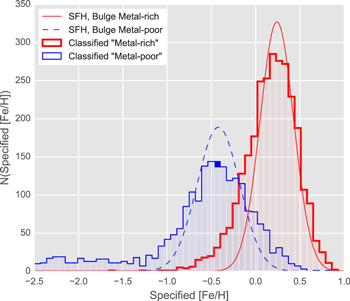
Figure 32. Comparison of recovered and input samples for the five-component BaSTI-based synthetic composite SWEEPS-field population (e.g., Figure 30). The histograms show the objects classified with the "metal-poor" (blue, thin stepped line) and "metal-rich" (red, thick stepped line) samples. The smooth Gaussian [Fe/H] distributions that were specified for the two bulge components are overlaid: the metal-poor (blue dashed curve) and the metal-rich (red solid curve) components. The [Fe/H] values are those reported in the BaSTI output tables (see the discussion in Appendix F). See Appendix E.
Download figure:
Standard image High-resolution imageE.5. The Impact of RV Variations
The framework of this appendix also allows us to investigate the impact of RV variations on ![$[t],[m]$](https://content.cld.iop.org/journals/0004-637X/858/1/46/revision1/apjaaba7fieqn404.gif) -based determinations. The extinction-free indices
-based determinations. The extinction-free indices ![$[t],[m]$](https://content.cld.iop.org/journals/0004-637X/858/1/46/revision1/apjaaba7fieqn405.gif) assume a particular extinction prescription (Cardelli et al. 1989, using
assume a particular extinction prescription (Cardelli et al. 1989, using  ). While
 ![$[t],[m]$](https://content.cld.iop.org/journals/0004-637X/858/1/46/revision1/apjaaba7fieqn407.gif) are therefore insensitive to variations in
are therefore insensitive to variations in  for a particular value of RV, variations in
  could impact the distribution of points in the
 ![$[t],[m]$](https://content.cld.iop.org/journals/0004-637X/858/1/46/revision1/apjaaba7fieqn410.gif) diagram, by altering the relationships between apparent magnitudes in the BTS filters and those assumed when computing
diagram, by altering the relationships between apparent magnitudes in the BTS filters and those assumed when computing ![$[t],[m]$](https://content.cld.iop.org/journals/0004-637X/858/1/46/revision1/apjaaba7fieqn411.gif) .
.
We appeal to the SWEEPS CMD to estimate limits on the magnitude of RV variations in this field. Assuming that the distance distribution due to the physical depth of the bulge can in this field be characterized by a Gaussian with width parameter σd kpc, the observed apparent magnitude scatter of RCGs in this field then sets an upper limit on  variations for assumed
  . In the SWEEPS data set, the observed F814W dispersion of the RCG is
  mag (Cl08).
For this appendix we adopt  = 0.5 (Ca14) as a representative value (the implied RV variations would become smaller for larger
  ). The extreme case of distance dispersion, σd = 0, then admits
  variation of
  . However, the bulge has nonzero depth along the line of sight; picking a representative distance distribution of
  suggests that variation closer to
  ≈ 0.25 is more likely. Both estimates for
  are conservative upper limits, since they ascribe none of the observed RCG apparent magnitude dispersion to photometric uncertainty, luminosity variations within the RCG sample, or
  variation.
To estimate the impact of  variation on the
 ![$[t],[m]$](https://content.cld.iop.org/journals/0004-637X/858/1/46/revision1/apjaaba7fieqn424.gif) distribution (and thus sample selection and cross-contamination), a synthetic population was constructed using BaSTI population components tuned to the estimated metallicity distribution for this field. Full details of this procedure, which was implemented to explore metallicity-dependent selection and characterization systematics (Section 5.1), can be found in Appendix E.
distribution (and thus sample selection and cross-contamination), a synthetic population was constructed using BaSTI population components tuned to the estimated metallicity distribution for this field. Full details of this procedure, which was implemented to explore metallicity-dependent selection and characterization systematics (Section 5.1), can be found in Appendix E.
Figure 33 shows the comparison of a simulated ![$[t],[m]$](https://content.cld.iop.org/journals/0004-637X/858/1/46/revision1/apjaaba7fieqn425.gif) population, with and without
population, with and without  variations at the
  level admitted by the SWEEPS data set. For each relevant WFC3 filter, the scale factors
  were estimated by linear interpolation in
  using information shown in Table 4. The simulated magnitudes were thus perturbed into "observed" magnitudes using different
  values for each star, but the
 ![$[t],[m]$](https://content.cld.iop.org/journals/0004-637X/858/1/46/revision1/apjaaba7fieqn431.gif) were computed using the
were computed using the  values appropriate for
  . This then mimics the use of a single
  value to compute
 ![$[t],[m]$](https://content.cld.iop.org/journals/0004-637X/858/1/46/revision1/apjaaba7fieqn435.gif) for a population that in reality shows
for a population that in reality shows  variations.
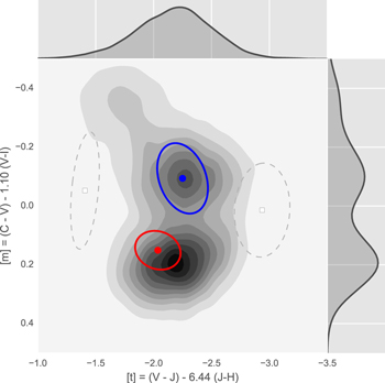
Figure 33. Estimating the impact of  variations in the
 ![$[t],[m]$](https://content.cld.iop.org/journals/0004-637X/858/1/46/revision1/apjaaba7fieqn438.gif) diagram. The top middle panel of Figure 28 shows a simulated
diagram. The top middle panel of Figure 28 shows a simulated ![$[t],[m]$](https://content.cld.iop.org/journals/0004-637X/858/1/46/revision1/apjaaba7fieqn439.gif) distribution using estimated photometric uncertainties and [Fe/H] distribution, and with RV = 2.5 for all objects. This figure shows the same simulation, but this time varying
distribution using estimated photometric uncertainties and [Fe/H] distribution, and with RV = 2.5 for all objects. This figure shows the same simulation, but this time varying  by
by  . The 1σ ellipses from the GMM decomposition of the observed data are shown to allow rough comparison between this simulation and the true data set, and the top and side panels show the marginal distributions of
 ![$[t]$](https://content.cld.iop.org/journals/0004-637X/858/1/46/revision1/apjaaba7fieqn442.gif) and
and ![$[m]$](https://content.cld.iop.org/journals/0004-637X/858/1/46/revision1/apjaaba7fieqn443.gif) , respectively. See Appendix E.5.
, respectively. See Appendix E.5.
Download figure:
Standard image High-resolution imageComparing the synthetic ![$[t],[m]$](https://content.cld.iop.org/journals/0004-637X/858/1/46/revision1/apjaaba7fieqn444.gif) distributions with and without
distributions with and without  variations (Figure 33), it seems unlikely that
  variations at the level admitted by the SWEEPS CMD can contribute a strong effect on GMM fitting or sample selection in
 ![$[t],[m]$](https://content.cld.iop.org/journals/0004-637X/858/1/46/revision1/apjaaba7fieqn447.gif) ; the impact of
; the impact of  variations is simply too small. We therefore proceed under the assumption that indeed
  for all objects in the SWEEPS field of view.
Appendix F: Testing the Behavior of the BaSTI Stellar Evolutionary Models
Because stars in the SWEEPS field likely span a very wide [Fe/H] range, including possibly objects outside the ranges traced by the BaSTI evolutionary models, we test the behavior of the BaSTI synthetic population framework when objects with very low or very high metallicities are simulated.
We find that BaSTI v5.0.1 appears to be imposing an internal truncation on the simulated populations, probably on [Fe/H] or on an internal variable that correlates with metallicity (for clarity, we refer to internal limits as [Fe/H] limits throughout this section). This in turn leads to a discrepancy between the requested and simulated population and between the reported [Fe/H] values in the simulated output and the resulting population. Since BaSTI is used very widely in studies of resolved stellar populations (with over 600 refereed citations), we report here our investigation into this truncation.37
A variety of synthetic populations were simulated using BaSTI's "user-specified SFH" option. This allows the user to build a population from a series of bursts of star formation, with the mean and standard deviation [Fe/H] specified for each population, as well as the number of years elapsed since the burst took place. In addition to the components that might make up the scene in the SWEEPS field of view (e.g., Appendix E.2), we simulated a number of "test-pattern" populations, with components regularly (or nearly regularly) spaced in [Fe/H].
The behavior of the CMD in the SWEEPS filters is then examined for consistency with the specified [Fe/H] distribution and also the [Fe/H] values reported in the simulated population. For regions in the CMD approximately near the selection region used in this communication, the absolute magnitude difference ΔM is computed from a fitted median sequence (in much the same manner as is done for the observed population), and the distribution of ΔM is examined for hard edges that are not present in the requested [Fe/H] distribution.
The BaSTI documentation was used to estimate median [Fe/H] values near the limits of its metallicity range.38 Specifically, we assumed the appropriate [Fe/H] limits to be −2.27 ≤ [Fe/H] ≤ +0.40 for scaled-to-solar models and −2.62 ≤ [Fe/H] ≤ +0.05 for α-enhanced models. Results for a representative set of test cases are reported below, which suggest the following effects:
- 1.Any bursts of star formation with specified median [Fe/H] outside internal limits are clipped to these limits before generation of the stellar population (Appendix F.1).
- 2.If the specified [Fe/H] distribution leads to individual objects with [Fe/H] outside the limits, the absolute magnitudes of these objects are truncated internally, but the reported [Fe/H] values appear to be unaffected, leading to a discrepancy between reported and applied [Fe/H] values (Appendix F.2).
- 3.The truncation behavior appears more complex than a simple clipping or substitution; discrepant objects can appear quite deep into the main body of the selected population, and the effective [Fe/H] limits might differ from those suggested by the documentation (Appendix F.3).
F.1. BaSTI Selection Applied to Median Populations
To investigate whether BaSTI is applying the truncation to the median population in a requested sample, test populations were simulated for bursts of star formation of equal magnitude but with very narrow [Fe/H] distributions. Figure 34 shows an example for a scaled-to-solar set of isochrones, with [Fe/H] = {−3.0, −2.5, −2.0, −1.5, −1.0, −0.5, +0.0, +0, 4, +0.5}, all with spread σ[Fe/H] = 0.0001 dex to isolate selection effects applied to the mean populations in each case. The two most metal-poor populations and the single most metal-rich population are found to be forced away from their specified values, probably to some internal limit. Reading off the figure, the most metal-poor populations seem to be brought up to [Fe/H] ≈ −2.3, with the most metal-rich brought down to [Fe/H] ≈ +0.40. These values are entirely consistent with the [Fe/H] limits suggested by the BaSTI documentation referenced earlier.
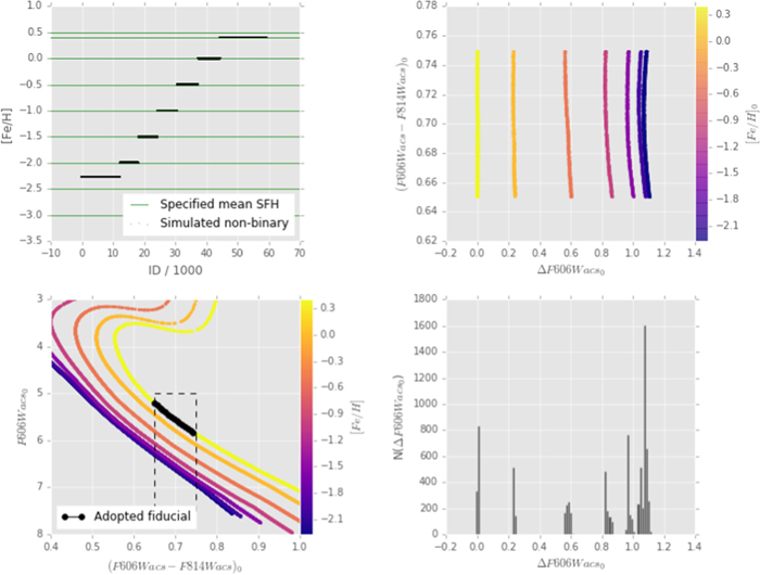
Figure 34. Testing the relationship between specified and simulated metallicities when bursts of star formation with a very wide range of median [Fe/H] values are requested with the BaSTI interface. Top left: specified and simulated [Fe/H] median values. The green horizontal lines show the median [Fe/H] values for the bursts of star formation, with the gray points indicating [Fe/H] values reported in the output simulation. In this example, specified bursts are ordered from bottom to top and left to right in the simulated objects. Bottom left: absolute magnitude CMD in the SWEEPS filters of the resulting population, color-coded by reported [Fe/H]. The black dots and line refer to the fitted fiducial in the selection region and a polynomial fit to the fiducial, respectively. Top right: absolute magnitude offsets ΔM from the adopted fiducial, ordered by SWEEPS color, with symbols color-coded by [Fe/H] reported in the simulated population. Bottom right: histogram of ΔM. Here the specified median [Fe/H] values were  , all with specified spread σ[Fe/H] = 0.0001 dex. Populations with [Fe/H] ≲ −2.3 or [Fe/H] ≳ +0.4 seem to have been wrapped by BaSTI to the metallicity limits. See Appendix F.1.
Download figure:
Standard image High-resolution imageThis suggests that BaSTI enforces [Fe/H] limits on the median populations requested in a simulation.
F.2. BaSTI Truncation near the [Fe/H] Limits
To investigate whether BaSTI applies a truncation to [Fe/H] values that are carried outside internal [Fe/H] limits owing to the specified population spread, test populations were simulated including a single population well away from the limits and one component each just inside the two limits. Components were specified with ![$[\mathrm{Fe}/{\rm{H}}]=\{-2.5,-1.2,+0.05\}$](https://content.cld.iop.org/journals/0004-637X/858/1/46/revision1/apjaaba7fieqn451.gif) , all with specified spread σ[Fe/H] = 0.1 dex, to ensure that the two components near the [Fe/H] limits each include substantial numbers of objects outside these limits, while the middle population has very few such objects.
, all with specified spread σ[Fe/H] = 0.1 dex, to ensure that the two components near the [Fe/H] limits each include substantial numbers of objects outside these limits, while the middle population has very few such objects.
Figure 35 shows the resulting simulation. Curiously, although the [Fe/H] values reported in the simulated populations show no truncation, the CMD and the simulated absolute magnitudes quite clearly do show truncation, with a hard edge at both the upper and lower [Fe/H] extrema.
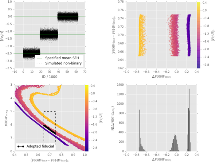
Figure 35. Testing the behavior of BaSTI simulations for populations with [Fe/H] close to the internal boundaries. Left column: panels and symbols as in Figure 34, with specified bursts ordered bottom to top and their simulated populations ordered left to right. Here a three-component α-enhanced population is simulated, with ![$[\mathrm{Fe}/{\rm{H}}]=\{-2.5,-1.2,+0.05\}$](https://content.cld.iop.org/journals/0004-637X/858/1/46/revision1/apjaaba7fieqn452.gif) , all with specified spread σ[Fe/H] = 0.1 dex. The metal-poor and metal-rich populations show sharp cutoffs in both the CMD and the ΔM distribution, which are not present in either the central population (well away from the [Fe/H] limits) or the reported [Fe/H] distributions of the metal-poor and metal-rich populations. (Curvature in the metal-poor hard edge is likely due to differences in the shape of the median population for [Fe/H] = −2.5 and that for [Fe/H] = −1.2.) The simulated magnitudes of the resulting populations show hard edges at the metal-rich and metal-poor ends, suggesting truncation in the delivered populations. Curiously, however, there is no such truncation in the corresponding reported [Fe/H] values. This suggests that a truncation is being applied after the assignment of [Fe/H] values to simulated objects. See Appendix F.2.
, all with specified spread σ[Fe/H] = 0.1 dex. The metal-poor and metal-rich populations show sharp cutoffs in both the CMD and the ΔM distribution, which are not present in either the central population (well away from the [Fe/H] limits) or the reported [Fe/H] distributions of the metal-poor and metal-rich populations. (Curvature in the metal-poor hard edge is likely due to differences in the shape of the median population for [Fe/H] = −2.5 and that for [Fe/H] = −1.2.) The simulated magnitudes of the resulting populations show hard edges at the metal-rich and metal-poor ends, suggesting truncation in the delivered populations. Curiously, however, there is no such truncation in the corresponding reported [Fe/H] values. This suggests that a truncation is being applied after the assignment of [Fe/H] values to simulated objects. See Appendix F.2.
Download figure:
Standard image High-resolution imageWe therefore find that BaSTI does not truncate [Fe/H] values at the stage of assignment to simulated objects, and these nontruncated [Fe/H] values are carried through to the output simulated population. However, a truncation is applied at some stage before the absolute magnitudes are included in the simulated population. This results in both a hard edge to the distribution of simulated absolute magnitudes and a discrepancy between the reported [Fe/H] values and the absolute magnitudes in the simulation output.
F.3. BaSTI Truncation near the Metal-rich Limit
To chart the behavior of the truncation near the [Fe/H] limits in more detail, we simulated a single test population near the metal-rich limit. Figure 36 shows the result for a scaled-to-solar component with [Fe/H] = +0.24 and scatter σ[Fe/H] = 0.19. In this case, the truncation appears to be quite dramatic, with a narrow, highly overrepresented component in the ΔM distribution.
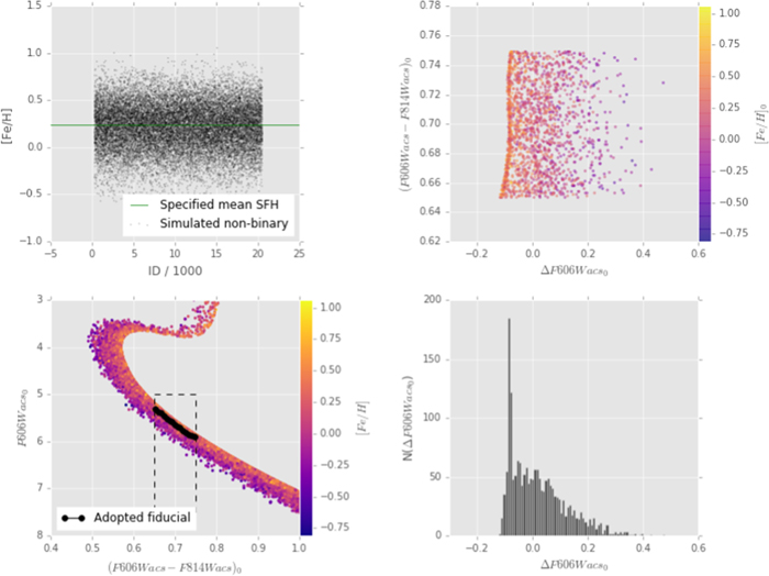
Figure 36. Charting detailed behavior of BaSTI truncation near the metal-rich limit. Panels and symbols are as in Figure 35; here a single scaled-to-solar component is simulated with [Fe/H] = +0.24 and scatter σ[Fe/H] = 0.19. A strong pileup is observed at the bright end of the ΔM distribution (curvature in this component is likely due to systematics in the determination of the fiducial ridgeline, which was determined from the simulated CMD, as would be the case for observed populations, rather than specified using an isochrone). Again, while a strong truncation is observed in the simulated absolute magnitudes, no such hard edge is present in the reported [Fe/H] values. See Appendix F.3 and Figure 31.
Download figure:
Standard image High-resolution imageHowever, the behavior of the simulator near an [Fe/H] limit is not as straightforward as a simple substitution of the [Fe/H] limit for all objects beyond it. Figure 31 shows a simulated metal-rich population partitioned by [Fe/H], which allows us to distinguish objects that were assigned [Fe/H] values above the metal-rich limit (and thus would be assumed to be truncated). Objects with outlier [Fe/H] values do not only appear at the location where absolute magnitudes pile up; a substantial fraction show magnitudes deeper into the main population (see the bottom left panel of Figure 31).
That the pileup implying truncation is also observed at the metal-rich edge of the population with simulated metallicities within the limits according to the BaSTI documentation suggests that the effective metallicity limits may differ from those documented; see the middle left panel of Figure 31. (We have not yet dissected this simulated population by binarity, which might offer another avenue for objects to wander into truncation territory.)
We therefore find that the internal truncation applied by BaSTI is not limited to a simple pegging of values to an internal boundary. The behavior probably necessitates some sort of selection on ΔM to produce a cleaner unaffected sample. We adopt one such approach in Appendix E.3.
Appendix G: Cross-contamination in the [t], [m] Diagram
We consider here the mixing of the "metal-rich" and "metal-poor" samples (and thus rotation curves) due to cross-contamination in the ![$[t]$](https://content.cld.iop.org/journals/0004-637X/858/1/46/revision1/apjaaba7fieqn453.gif) ,
, ![$[m]$](https://content.cld.iop.org/journals/0004-637X/858/1/46/revision1/apjaaba7fieqn454.gif) space from which the two samples were drawn (Section 5.2).
space from which the two samples were drawn (Section 5.2).
While the formal membership probability threshold  ≥
≥  was chosen to be somewhat conservative, some amount of sample contamination in
 ![$[t]$](https://content.cld.iop.org/journals/0004-637X/858/1/46/revision1/apjaaba7fieqn457.gif) ,
, ![$[m]$](https://content.cld.iop.org/journals/0004-637X/858/1/46/revision1/apjaaba7fieqn458.gif) is highly likely. Since the (
is highly likely. Since the (![$[t],[m]$](https://content.cld.iop.org/journals/0004-637X/858/1/46/revision1/apjaaba7fieqn459.gif) ) each represent flux ratios constructed from photometry in three filters, it is likely that objects best characterized at one side of the abundance range for the bulge might be classified to an object in the other owing to photometric uncertainty. In principle, a nearly flat rotation curve for one sample could be polluted by samples from another sample with a large-amplitude rotation curve, and vice versa, sufficiently to weaken the trends in the high-amplitude sample while imprinting a signal on the other that is not in fact present.
) each represent flux ratios constructed from photometry in three filters, it is likely that objects best characterized at one side of the abundance range for the bulge might be classified to an object in the other owing to photometric uncertainty. In principle, a nearly flat rotation curve for one sample could be polluted by samples from another sample with a large-amplitude rotation curve, and vice versa, sufficiently to weaken the trends in the high-amplitude sample while imprinting a signal on the other that is not in fact present.
A rigorous exploration of the cross-contamination in (![$[t],[m]$](https://content.cld.iop.org/journals/0004-637X/858/1/46/revision1/apjaaba7fieqn460.gif) ) requires a somewhat involved set of computations. For example, flat priors in observed flux (for each of the five filters used in BTS) are unlikely to translate into flat priors in (
) requires a somewhat involved set of computations. For example, flat priors in observed flux (for each of the five filters used in BTS) are unlikely to translate into flat priors in (![$[t],[m]$](https://content.cld.iop.org/journals/0004-637X/858/1/46/revision1/apjaaba7fieqn461.gif) ) space, as suggested graphically by the degeneracy exhibited by very metal-poor populations in the (
) space, as suggested graphically by the degeneracy exhibited by very metal-poor populations in the (![$[t],[m]$](https://content.cld.iop.org/journals/0004-637X/858/1/46/revision1/apjaaba7fieqn462.gif) ) diagram (e.g., Brown et al. 2009). To properly account for cross-contamination likely requires simulations of the underlying metallicity and temperature distributions (for which a range of shape parameters for the distributions would also need exploration) and then translating them forward into the probability density function in (
) diagram (e.g., Brown et al. 2009). To properly account for cross-contamination likely requires simulations of the underlying metallicity and temperature distributions (for which a range of shape parameters for the distributions would also need exploration) and then translating them forward into the probability density function in (![$[t],[m]$](https://content.cld.iop.org/journals/0004-637X/858/1/46/revision1/apjaaba7fieqn463.gif) ), including full accounting for the shape of the measurement uncertainty distributions and covariances in each of the filters. We consider this beyond the scope of the present work.
), including full accounting for the shape of the measurement uncertainty distributions and covariances in each of the filters. We consider this beyond the scope of the present work.
Instead, we have performed a simpler quantitative estimate of the degree of cross-contamination in (![$[t],[m]$](https://content.cld.iop.org/journals/0004-637X/858/1/46/revision1/apjaaba7fieqn464.gif) ) space. We assume that the four-component GMM is indeed a reasonable characterization of the observed distribution of (
) space. We assume that the four-component GMM is indeed a reasonable characterization of the observed distribution of (![$[t],[m]$](https://content.cld.iop.org/journals/0004-637X/858/1/46/revision1/apjaaba7fieqn465.gif) ) values, and also that the measurement uncertainties in this space can be described as 2D Gaussians for each object. Samples in (
) values, and also that the measurement uncertainties in this space can be described as 2D Gaussians for each object. Samples in (![$[t],[m]$](https://content.cld.iop.org/journals/0004-637X/858/1/46/revision1/apjaaba7fieqn466.gif) ) are simulated by drawing from the best-fit four-component GMM and perturbing each object by an uncertainty covariance matrix (Equation (4)) drawn randomly without replacement from the observed population. Then a four-component GMM is fit to each sample, and objects are classified to belong to a model component using the
) are simulated by drawing from the best-fit four-component GMM and perturbing each object by an uncertainty covariance matrix (Equation (4)) drawn randomly without replacement from the observed population. Then a four-component GMM is fit to each sample, and objects are classified to belong to a model component using the  ≥
≥  threshold that was used on the observed data set (an object cannot satisfy this condition for more than one model component by construction). Finally, the model component classification for each object is compared to the model component from which it was originally drawn, to measure the contamination for each component (i.e., the fraction of objects classified with component K but drawn from
  ).
).
Figure 37 shows the results of 5000 simulation sets. Generally, the "metal-poor" component is relatively uncontaminated by any other population; the total contamination from these simulations is ≤1% in all the trials, with the strongest contamination contributed by the "metal-rich" component (at ∼0.1%–0.8%). The "metal-rich" component is more strongly contaminated. Roughly 5% of this sample is contaminated by the "metal-poor" component, which is the dominant contaminant (the two background components together providing less than 0.5% in all trials).
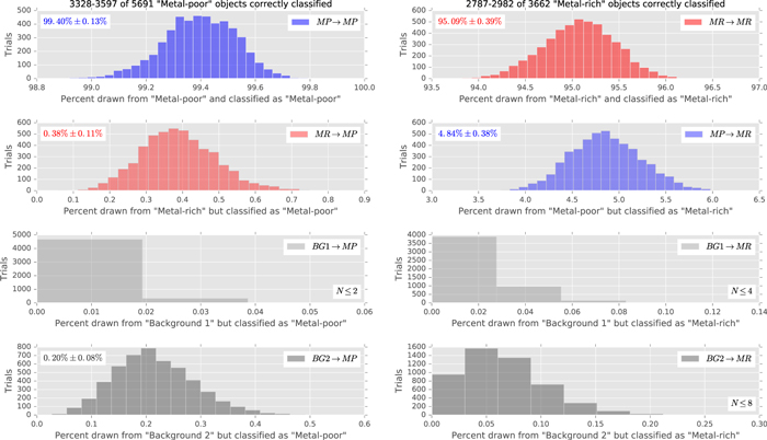
Figure 37. Simple Monte Carlo test for cross-contamination of the "metal-rich" and "metal-poor" samples in (![$[t],[m]$](https://content.cld.iop.org/journals/0004-637X/858/1/46/revision1/apjaaba7fieqn470.gif) ) space. Objects are simulated from the best-fit four-component GMM in (
) space. Objects are simulated from the best-fit four-component GMM in (![$[t],[m]$](https://content.cld.iop.org/journals/0004-637X/858/1/46/revision1/apjaaba7fieqn471.gif) ) space (whose parameters are given in Table 5), perturbed by measurement uncertainty, and re-characterized using another four-component GMM and classified by membership probability (
) space (whose parameters are given in Table 5), perturbed by measurement uncertainty, and re-characterized using another four-component GMM and classified by membership probability ( ) in the same way as the observed data (Section 3.5). The model component assigned to each object in the characterization is then compared to the component from which the object was drawn. Each panel shows the distribution of trials (out of 5000 total) in which a given percentage of objects were classified with the indicated mixture component. The left column shows the distribution of origin components for objects classified as "metal-poor" (top left, blue); the right column shows the origin components for objects classified as "metal-rich" (top right, red). In each column the top panel shows the distributions of objects classified correctly, while the others show the distributions of objects classified with a different (indicated) component. Only a handful of objects from the "Background-1" component (k = 2 in Table 5) are misidentified with either the "metal-rich" or the "metal-poor" sample in any of the trials. See Appendix G.
Download figure:
Standard image High-resolution imageThese ranges almost certainly underestimate the true contamination between samples in (![$[t],[m]$](https://content.cld.iop.org/journals/0004-637X/858/1/46/revision1/apjaaba7fieqn473.gif) ). The observed (
). The observed (![$[t],[m]$](https://content.cld.iop.org/journals/0004-637X/858/1/46/revision1/apjaaba7fieqn474.gif) ) distribution tends to be less centrally peaked than the model samples (Figure 20), suggesting that the model likely generates samples whose classification by
) distribution tends to be less centrally peaked than the model samples (Figure 20), suggesting that the model likely generates samples whose classification by ![$[t],[m]$](https://content.cld.iop.org/journals/0004-637X/858/1/46/revision1/apjaaba7fieqn475.gif) is artificially less vulnerable to contamination than in reality. Furthermore, even if the distribution in flux ratio due to measurement uncertainty is Gaussian for a given filter, for uncertainties
is artificially less vulnerable to contamination than in reality. Furthermore, even if the distribution in flux ratio due to measurement uncertainty is Gaussian for a given filter, for uncertainties  the apparent magnitude uncertainty distribution will deviate substantially from a Gaussian.
Full exploration of these effects is deferred to future work. For the present, our limited simulation suggests that the two samples are contaminated in (![$[t],[m]$](https://content.cld.iop.org/journals/0004-637X/858/1/46/revision1/apjaaba7fieqn477.gif) ) at the ≲5% level, using the
) at the ≲5% level, using the  ≥
≥  threshold for classification.
Appendix H: Cross-comparison between Catalog Versions
While this work was at an advanced stage, a second version of the BTS catalog (hereafter "BTSv2") was released to the HST archive, based on a re-analysis of the first-epoch BTS data using improved measurement methods.39 The comparison of BTSv2 to the first catalog version (hereafter "BTSv1") helps prepare the ground for the ongoing investigations discussed in Section 6, and so we present the comparison here.
Appendix H.1 compares the apparent magnitudes of the two catalogs, while Appendix H.2 compares the SWEEPS proper motions with the BTSv2 proper motions. In Appendix H.3 the two catalogs are compared against the absolute reference frame provided by the first Gaia data release (which contains positions but not proper motions for these objects). Finally, in Appendix H.4 we present a preliminary re-determination of the proper-motion rotation curves using BTSv2 data exclusively.
H.1. Photometry Comparision between BTSv2 and BTSv1
The BTSv1 photometric catalog was produced using daophotII on summed images in each filter before combining into the final catalog (Section 2.2 and references therein), while the BTSv2 catalog uses "effective PSF" methods (e.g., Anderson & King 2006), the details of which vary depending on the brightness regime of the object used. Objects in the brightness range of our proper-motion sample (Figure 2) were measured using the kstwo code by J. Anderson, which fits position and flux for each star across all exposures simultaneously (see Bellini et al. 2017, for details). For sufficiently bright and isolated objects, the source position and flux were fit independently, while for fainter and/or less isolated stars the flux was measured using forced photometry (with the star position fixed). Because both the source brightness and degree of isolation depend on the filter and camera used, a given star might be measured using forced photometry in some filters but not others.
Figure 38 presents the comparison of apparent magnitude between BTSv2 and BTSv1, over the apparent magnitude range of interest to the present work (stars were cross-matched between the two catalogs using their equatorial coordinates). The random component of the apparent magnitude difference is  mag in all filters for most objects (compare with the apparent magnitude selection criteria in Table 3). Systematic offsets between the data sets are less than 0.02 mag.
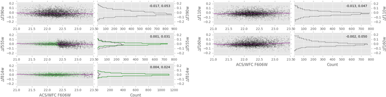
Figure 38. Apparent magnitude comparison between the BTS v1 and v2 photometric catalogs for cross-matched objects within our sample of interest (see Figure 2). Each pair of panels presents the difference in apparent magnitude (in the Vegamag system), in the sense (v2–v1), showing the run against SWEEPS apparent magnitude (scatterplots) and the marginal distributions (histograms). Small green symbols and green solid lines represent objects whose flux and position were measured independently in BTSv2, while larger gray symbols and the gray dashed lines represent objects whose flux was measured at a fixed position. In the scatterplots, median trends are shown with a solid line. The inset annotations give the median and standard deviation of the magnitude differences. The left-hand set of panels represents the comparison for WFC3/UVIS, while the right-hand set represents WFC3/IR. For a discussion, see Appendix H.1.
Download figure:
Standard image High-resolution imageH.2. Proper-motion Comparison between BTSv2 and SWEEPS
Figure 39 presents the star-by-star proper-motion comparison between the BTSv2 and SWEEPS catalog for objects in our apparent magnitude range of interest. Any difference in scale between the proper-motion determinations is below 1%. A small offset  ≈
≈  between the two catalogs is apparent, as expected if the proper-motion zero-point of the two catalogs depends ultimately on the differing depth of the two surveys. The proper-motion differences show rms scatter
  mas yr−1. Assuming that the full SWEEPS proper motions carry uncertainty
  mas yr−1 (Appendix A), the BTSv2 proper motions for this field would contribute approximately BTS ≈ 0.27 mas yr−1. No trend in the proper-motion differences was found against apparent magnitude, proper motion, or position.
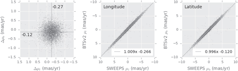
Figure 39. Comparison of the BTSv2 and SWEEPS proper motions, for objects in our sample of interest (Figure 2). The left panel shows the proper-motion differences (in the sense BTSv2–SWEEPS), with the mean proper-motion offset between the two catalogs indicated by the cross-hair and annotation; the rms scatter in (Δμl, Δμb) is (0.28, 0.29) mas yr−1. The middle and right panels plot the proper motions against each other and present the best-fit straight-line models, in Galactic longitude (middle) and latitude (right). See the discussion in Appendix H.2.
Download figure:
Standard image High-resolution imageH.3. Astrometric Reference-frame Comparison with Gaia DR1
To check the orientation of the astrometric frames of the catalogs, positions in the SWEEPS and BTSv2 catalogs were matched to their entries in the First Gaia Data Release, which should provide absolute positions on the International Celestial Reference System (ICRS) in the 2015.0 epoch, albeit possibly with residual distortions in these crowded regions (Gaia Collaboration et al. 2016a, 2016b). Objects in the Gaia apparent magnitude range  were selected for cross-matching, as a trade-off between quality of Gaia measurement and the desire to avoid highly saturated objects in the SWEEPS and BTS catalogs; this leaves a few thousand objects with which to probe positional differences. To minimize random scatter in the comparison, positions from the SWEEPS and BTSv2 catalogs were advanced to their positions in the 2015.0 epoch using the measured proper motions in each catalog; the Gaia DR1 catalog does not contain proper motions for these objects.
Figure 40 maps the astrometric offsets from the Gaia DR1 frame for both the SWEEPS and BTS catalogs. While the two catalogs are slightly offset with respect to the Gaia DR1 frame (by  in each coordinate), no rotational flow pattern is detected that would suggest misalignment of either of the reference frames. The scale of the positional residuals is surprisingly large, with flow pattern common to both catalog comparisons that reaches up to
  in some regions. The largest residual structure is found at a similar location in the comparisons to both the SWEEPS and BTSv2 catalogs, despite the two HST catalogs being taken at different camera orientations and with different field centers, so we suspect that the flow pattern is dominated by distortion in the Gaia DR1 frame in these crowded regions. (Comparison of Subaru measurements with Gaia DR1 positions near the core of the Sextans dwarf galaxy also shows a flow pattern of offsets on a scale of
  with a gap in Gaia DR1 coverage; C. Dinescu 2018, private communication.) We expect that this flow pattern will vanish in comparisons to future Gaia data releases that have included the more sophisticated treatment for crowding outlined in Pancino et al. (2017). Based on the scale of the flow patterns near the corners of the difference maps (≲01), we conclude that the astrometric reference frames of the SWEEPS and BTSv2 catalogs are aligned with the ICRS frame to better than ∼005.
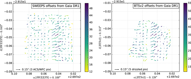
Figure 40. Checking the astrometric reference frame of the SWEEPS and BTSv2 catalogs by comparing bright-star positions to the first Gaia Data Release (Gaia Collaboration et al. 2016a, 2016b). Panels show positional offsets between Gaia DR1 and the SWEEPS (left panel) and BTSv2 (right panel) catalogs. Vectors show the median positional offsets of image regions with at least 10 stars matched with Gaia DR1 (the shading indicates the number of cross-matched stars per region). Median offsets in arcseconds are indicated in the axis labels. While substantial residual structure is present in both sets of offsets, no frame rotation is detected at the ≲005 level, for either catalog. See the discussion in Appendix H.3.
Download figure:
Standard image High-resolution imageH.4. Preliminary Results Using BTSv2 Only
Finally, to investigate whether our results qualitatively change when moving from BTSv1 to BTSv2, we have performed a preliminary re-analysis using the BTSv2 measurements only, following the procedures of Section 3 as far as the production of the proper-motion rotation curves.
Not all the selection steps are common to both catalogs; for example, BTSv2 does not contain F606W measurements (as were used when we melded the SWEEPS and BTSv2 catalogs in Section 3), which thus alters the initial selection of objects, and BTSv2 contains additional information that can be used to select objects by measurement quality (details can be found in the BTSv2 README file). Additionally, BTSv2 proper-motion uncertainties have not yet been characterized as fully as the ACS/WFC uncertainties in the SWEEPS field (e.g., Calamida et al. 2015). Finally, the proper-motion zero-points of the two catalogs differ, and the appropriate value of  to use for BTSv2 has not yet been established.
Figure 41 shows the results. While some of the fine structure in the rotation curves appears to differ when compared to the BTSv1-based analysis, the behavior we observe is not substantially changed by use of the BTSv2 catalog; the "metal-rich" and "metal-poor" rotation curves still differ, with the "metal-rich" curve showing a steeper gradient. Full development of the chemically dissected bulge rotation curves will be reported in a future communication after the work has been extended to all four BTS fields.
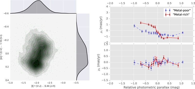
Figure 41. Preliminary re-analysis using BTSv2 data only, for both the ![$[t],[m]$](https://content.cld.iop.org/journals/0004-637X/858/1/46/revision1/apjaaba7fieqn490.gif) and the proper motions. Left panel: (
and the proper motions. Left panel: (![$[t],[m]$](https://content.cld.iop.org/journals/0004-637X/858/1/46/revision1/apjaaba7fieqn491.gif) ) distribution from the revised photometry (compare with Figure 3). Right panel: proper-motion rotation curve for "metal-rich" and "metal-poor" samples using BTSv2 proper motions (compare with Figure 8). See Appendix H.4 for discussion.
) distribution from the revised photometry (compare with Figure 3). Right panel: proper-motion rotation curve for "metal-rich" and "metal-poor" samples using BTSv2 proper motions (compare with Figure 8). See Appendix H.4 for discussion.
Download figure:
Standard image High-resolution imageAppendix I: Rotation Curves and Bin Statistics in Tabular Form
Tables 12–15 present the variation of the proper motion ellipse with distance, for the "Metal-rich" (Tables 12 and 13) and "Metal-poor samples (Tables 14 & 15). The bin statistics for the fine-grained binning scheme are presented in Tables 16 and 17.
Table 12. Observed Rotation Trend for the "Metal-rich" Sample, with Uncertainty Ranges Given as 1σ Limits Based on 1000 Parametric Bootstrap Trials
| π' | Bin Edges | N |

|

|
aμ | bμ | ϕlb | a/b |

|

|
Clb |
|---|---|---|---|---|---|---|---|---|---|---|---|
| (mag) | (mag) | (mas yr−1) | (mas yr−1) | (mas yr−1) | (mas yr−1) | (deg) | (mas2 yr−2) | (mas2 yr−2) | (mas2 yr−2) | ||
| −1.30 | −1.51, −1.18 | 20 | 2.96 ± 0.591 | −0.01 ± 0.287 | 2.6 ± 0.42 | 1.3 ± 0.21 | 0.8 ± 10.33 | 2.00 ± 0.112 | 6.88 ± 2.203 | 1.71 ± 0.535 | −0.07 ± 0.760 |
| −0.67 | −1.17, −0.48 | 198 | 1.58 ± 0.193 | −0.18 ± 0.160 | 2.8 ± 0.14 | 2.2 ± 0.11 | 21.3 ± 7.69 | 1.30 ± 0.053 | 7.52 ± 0.758 | 5.10 ± 0.512 | −1.11 ± 0.434 |
| −0.37 | −0.48, −0.31 | 199 | 1.14 ± 0.188 | −0.06 ± 0.161 | 2.7 ± 0.14 | 2.2 ± 0.11 | 25.5 ± 12.34 | 1.20 ± 0.058 | 6.81 ± 0.695 | 5.45 ± 0.543 | −0.84 ± 0.445 |
| −0.26 | −0.31, −0.22 | 199 | 1.13 ± 0.195 | 0.11 ± 0.206 | 3.0 ± 0.15 | 2.5 ± 0.12 | 52.7 ± 15.78 | 1.19 ± 0.056 | 8.03 ± 0.752 | 7.32 ± 0.813 | −1.28 ± 0.539 |
| −0.18 | −0.22, −0.15 | 196 | 1.17 ± 0.182 | −0.15 ± 0.197 | 2.8 ± 0.14 | 2.4 ± 0.12 | 59.1 ± 25.80 | 1.16 ± 0.055 | 7.45 ± 0.664 | 6.50 ± 0.758 | −0.88 ± 0.480 |
| −0.12 | −0.15, −0.10 | 199 | 1.14 ± 0.203 | −0.08 ± 0.182 | 3.0 ± 0.14 | 2.4 ± 0.12 | 30.5 ± 9.48 | 1.25 ± 0.055 | 8.34 ± 0.785 | 6.73 ± 0.653 | −1.45 ± 0.544 |
| −0.07 | −0.10, −0.04 | 199 | 0.80 ± 0.228 | 0.21 ± 0.205 | 3.2 ± 0.16 | 2.7 ± 0.13 | 34.7 ± 13.36 | 1.18 ± 0.055 | 9.48 ± 0.977 | 8.43 ± 0.837 | −1.40 ± 0.627 |
| −0.01 | −0.04, 0.02 | 199 | −0.00 ± 0.222 | 0.26 ± 0.189 | 3.3 ± 0.16 | 2.5 ± 0.12 | 32.3 ± 8.48 | 1.29 ± 0.053 | 9.43 ± 0.977 | 7.64 ± 0.754 | −1.90 ± 0.611 |
| 0.04 | 0.02, 0.06 | 197 | 0.00 ± 0.208 | 0.20 ± 0.193 | 3.1 ± 0.16 | 2.6 ± 0.13 | 36.4 ± 15.91 | 1.18 ± 0.057 | 8.37 ± 0.879 | 7.59 ± 0.773 | −1.27 ± 0.572 |
| 0.09 | 0.06, 0.12 | 199 | −0.68 ± 0.197 | 0.46 ± 0.203 | 3.1 ± 0.15 | 2.5 ± 0.12 | 41.0 ± 8.84 | 1.27 ± 0.054 | 8.12 ± 0.816 | 7.61 ± 0.766 | −1.84 ± 0.568 |
| 0.15 | 0.12, 0.18 | 198 | −0.93 ± 0.177 | 0.42 ± 0.190 | 2.9 ± 0.14 | 2.2 ± 0.11 | 50.1 ± 8.03 | 1.30 ± 0.051 | 6.87 ± 0.627 | 6.26 ± 0.671 | −1.67 ± 0.466 |
| 0.22 | 0.18, 0.26 | 198 | −1.03 ± 0.164 | 0.29 ± 0.165 | 2.4 ± 0.10 | 2.3 ± 0.10 | 63.3 ± 54.11 | 1.03 ± 0.045 | 5.47 ± 0.515 | 5.28 ± 0.550 | −0.12 ± 0.373 |
| 0.33 | 0.26, 0.41 | 198 | −1.10 ± 0.152 | 0.00 ± 0.138 | 2.2 ± 0.11 | 1.9 ± 0.09 | 31.8 ± 21.84 | 1.13 ± 0.053 | 4.50 ± 0.470 | 4.04 ± 0.413 | −0.46 ± 0.291 |
| 0.53 | 0.41, 1.25 | 134 | −0.98 ± 0.140 | 0.11 ± 0.141 | 1.6 ± 0.08 | 1.6 ± 0.08 | −65.1 ± 55.84 | 1.03 ± 0.049 | 2.63 ± 0.299 | 2.54 ± 0.322 | 0.05 ± 0.214 |
Note.  ,
,  represent the mean proper motions in each bin, with aμ, bμ the major and minor axes of the velocity ellipse, respectively. ϕlb gives the position angle (in l, b) of the proper-motion ellipse and a/b its major-axis:minor-axis ratio. Finally, the quantities
  , and Clb represent the three unique components of the proper-motion dispersion. See the discussion in Section 4.1.
Download table as: ASCIITypeset image
Table 13. Same as Table 12, but with Photometric Parallaxes and Proper Motions Converted into Distances and Velocities Using a Reference Distance of 7.76 kpc
| d |

|
N |

|

|
av | bv | ϕlb | a/b |

|

|

|
|---|---|---|---|---|---|---|---|---|---|---|---|
| (kpc) | (kpc) | (km s−1) | (km s−1) | (km s−1) | (km s−1) | (deg) | (km2 s−2) | (km2 s−2) | (km2 s−2) | ||
| 4.26 | 3.87,4.51 | 20 | 59.73 ± 11.939 | −0.28 ± 5.786 | 53 ± 8.4 | 26 ± 4.2 | 0.8 ± 10.33 | 2.00 ± 0.112 | 138.9 ± 44.48 | 34.6 ± 10.80 | −1.5 ± 15.34 |
| 5.69 | 4.53, 6.21 | 198 | 42.65 ± 5.198 | −4.94 ± 4.326 | 76 ± 3.8 | 58 ± 2.9 | 21.3 ± 7.69 | 1.30 ± 0.053 | 202.6 ± 20.42 | 137.6 ± 13.81 | −29.8 ± 11.70 |
| 6.55 | 6.22, 6.72 | 199 | 35.56 ± 5.850 | −1.84 ± 5.003 | 83 ± 4.2 | 70 ± 3.5 | 25.5 ± 12.34 | 1.20 ± 0.058 | 211.6 ± 21.59 | 169.2 ± 16.88 | −26.1 ± 13.82 |
| 6.90 | 6.72, 7.02 | 199 | 36.87 ± 6.390 | 3.48 ± 6.723 | 98 ± 4.9 | 82 ± 4.0 | 52.7 ± 15.78 | 1.19 ± 0.056 | 262.6 ± 24.59 | 239.4 ± 26.59 | −42.0 ± 17.62 |
| 7.14 | 7.02, 7.23 | 196 | 39.71 ± 6.163 | −5.06 ± 6.656 | 96 ± 4.6 | 83 ± 4.0 | 59.1 ± 25.80 | 1.16 ± 0.055 | 252.0 ± 22.47 | 219.9 ± 25.64 | −29.9 ± 16.25 |
| 7.33 | 7.23, 7.42 | 199 | 39.69 ± 7.058 | −2.84 ± 6.330 | 105 ± 5.0 | 84 ± 4.1 | 30.5 ± 9.48 | 1.25 ± 0.055 | 289.8 ± 27.29 | 234.1 ± 22.70 | −50.4 ± 18.90 |
| 7.51 | 7.42, 7.62 | 199 | 28.35 ± 8.121 | 7.48 ± 7.290 | 115 ± 5.9 | 97 ± 4.5 | 34.7 ± 13.36 | 1.18 ± 0.055 | 337.3 ± 34.78 | 299.9 ± 29.78 | −49.8 ± 22.31 |
| 7.71 | 7.62, 7.82 | 199 | −0.17 ± 8.097 | 9.63 ± 6.920 | 119 ± 6.0 | 93 ± 4.5 | 32.3 ± 8.48 | 1.29 ± 0.053 | 344.6 ± 35.72 | 279.1 ± 27.54 | −69.3 ± 22.32 |
| 7.90 | 7.82, 7.99 | 197 | 0.07 ± 7.775 | 7.36 ± 7.235 | 114 ± 5.9 | 97 ± 4.7 | 36.4 ± 15.91 | 1.18 ± 0.057 | 313.5 ± 32.91 | 284.1 ± 28.95 | −47.4 ± 21.43 |
| 8.10 | 7.99, 8.20 | 199 | −26.04 ± 7.561 | 17.79 ± 7.789 | 120 ± 5.9 | 94 ± 4.7 | 41.0 ± 8.84 | 1.27 ± 0.054 | 311.7 ± 31.33 | 292.0 ± 29.41 | −70.5 ± 21.80 |
| 8.30 | 8.20, 8.44 | 198 | −36.52 ± 6.951 | 16.47 ± 7.486 | 113 ± 5.5 | 87 ± 4.2 | 50.1 ± 8.03 | 1.30 ± 0.051 | 270.3 ± 24.67 | 246.5 ± 26.42 | −65.8 ± 18.32 |
| 8.58 | 8.44, 8.75 | 198 | −41.91 ± 6.672 | 11.88 ± 6.714 | 96 ± 4.1 | 93 ± 4.0 | 63.3 ± 54.11 | 1.03 ± 0.045 | 222.4 ± 20.95 | 214.9 ± 22.37 | −5.0 ± 15.17 |
| 9.02 | 8.75, 9.35 | 198 | −47.09 ± 6.515 | 0.04 ± 5.912 | 93 ± 4.5 | 83 ± 3.9 | 31.8 ± 21.84 | 1.13 ± 0.053 | 192.2 ± 20.10 | 172.7 ± 17.64 | −19.6 ± 12.46 |
| 9.89 | 9.36, 13.82 | 134 | −45.84 ± 6.561 | 5.37 ± 6.624 | 76 ± 3.8 | 74 ± 3.7 | −65.1 ± 55.84 | 1.03 ± 0.049 | 123.3 ± 14.03 | 119.1 ± 15.10 | 2.5 ± 10.05 |
Note. See the discussion in Section 4.1.
Download table as: ASCIITypeset image
Table 14. Observed Rotation Trend for the "Metal-poor" Sample, with Uncertainty Ranges Given as 1σ Limits Based on 1000 Parametric Bootstrap Trials
| π' | Bin Edges | N |

|

|
aμ | bμ | ϕlb | a/b |

|

|
Clb |
|---|---|---|---|---|---|---|---|---|---|---|---|
| (mag) | (mag) | (mas yr−1) | (mas yr−1) | (mas yr−1) | (mas yr−1) | (deg) | (mas2 yr−2) | (mas2 yr−2) | (mas2 yr−2) | ||
| −1.65 | −1.83, −1.42 | 20 | 2.96 ± 0.544 | 0.69 ± 0.641 | 3.2 ± 0.49 | 2.0 ± 0.30 | −55.2 ± 20.77 | 1.61 ± 0.125 | 8.41 ± 1.895 | 6.15 ± 2.686 | 3.03 ± 1.676 |
| −1.01 | −1.39, −0.79 | 199 | 0.57 ± 0.238 | −0.04 ± 0.210 | 3.3 ± 0.16 | 2.8 ± 0.13 | 22.9 ± 12.17 | 1.20 ± 0.054 | 10.52 ± 1.039 | 8.15 ± 0.834 | −1.22 ± 0.649 |
| −0.65 | −0.78, −0.56 | 198 | 0.61 ± 0.214 | −0.34 ± 0.211 | 3.4 ± 0.17 | 2.6 ± 0.13 | 40.6 ± 9.08 | 1.29 ± 0.053 | 9.47 ± 0.984 | 8.76 ± 0.868 | −2.27 ± 0.659 |
| −0.47 | −0.56, −0.39 | 198 | 0.38 ± 0.223 | −0.05 ± 0.223 | 3.5 ± 0.17 | 2.5 ± 0.12 | 43.8 ± 6.82 | 1.37 ± 0.052 | 9.40 ± 0.934 | 9.16 ± 0.892 | −2.81 ± 0.686 |
| −0.33 | −0.39, −0.29 | 199 | 0.30 ± 0.224 | −0.26 ± 0.208 | 3.2 ± 0.15 | 2.8 ± 0.13 | 14.3 ± 18.70 | 1.14 ± 0.053 | 10.32 ± 1.012 | 8.16 ± 0.809 | −0.59 ± 0.645 |
| −0.24 | −0.29, −0.20 | 198 | 0.14 ± 0.223 | 0.42 ± 0.216 | 3.2 ± 0.15 | 3.0 ± 0.13 | 29.9 ± 33.12 | 1.08 ± 0.049 | 9.75 ± 1.014 | 9.05 ± 0.904 | −0.59 ± 0.632 |
| −0.16 | −0.20, −0.13 | 198 | 0.18 ± 0.223 | 0.14 ± 0.217 | 3.4 ± 0.16 | 2.9 ± 0.14 | 50.4 ± 24.56 | 1.15 ± 0.054 | 10.29 ± 0.980 | 9.75 ± 1.063 | −1.40 ± 0.721 |
| −0.09 | −0.13, −0.04 | 196 | −0.01 ± 0.208 | 0.10 ± 0.212 | 3.1 ± 0.15 | 2.8 ± 0.13 | 50.3 ± 26.77 | 1.13 ± 0.054 | 8.95 ± 0.842 | 8.55 ± 0.878 | −1.06 ± 0.622 |
| −0.01 | −0.04, 0.02 | 199 | −0.15 ± 0.215 | 0.48 ± 0.188 | 3.0 ± 0.14 | 2.6 ± 0.13 | 13.9 ± 20.05 | 1.14 ± 0.055 | 8.84 ± 0.873 | 6.97 ± 0.709 | −0.49 ± 0.552 |
| 0.06 | 0.03, 0.09 | 200 | −0.35 ± 0.210 | 0.08 ± 0.195 | 3.2 ± 0.15 | 2.8 ± 0.14 | 22.9 ± 17.39 | 1.15 ± 0.056 | 9.75 ± 0.962 | 8.03 ± 0.784 | −0.89 ± 0.629 |
| 0.13 | 0.09, 0.17 | 197 | −0.38 ± 0.198 | 0.02 ± 0.194 | 2.8 ± 0.12 | 2.8 ± 0.11 | 59.5 ± 53.65 | 1.02 ± 0.044 | 7.84 ± 0.746 | 7.68 ± 0.771 | −0.15 ± 0.551 |
| 0.21 | 0.17, 0.26 | 197 | −0.63 ± 0.231 | 0.28 ± 0.196 | 3.2 ± 0.16 | 2.7 ± 0.13 | −10.7 ± 15.33 | 1.17 ± 0.055 | 10.20 ± 1.026 | 7.60 ± 0.765 | 0.51 ± 0.639 |
| 0.32 | 0.26, 0.37 | 199 | −0.58 ± 0.161 | 0.28 ± 0.190 | 2.7 ± 0.13 | 2.1 ± 0.10 | 63.7 ± 12.58 | 1.28 ± 0.053 | 6.72 ± 0.487 | 5.01 ± 0.690 | −1.12 ± 0.416 |
| 0.44 | 0.37, 0.54 | 197 | −0.65 ± 0.188 | 0.21 ± 0.173 | 2.5 ± 0.11 | 2.5 ± 0.10 | 11.2 ± 43.30 | 1.03 ± 0.043 | 6.46 ± 0.668 | 6.08 ± 0.592 | −0.08 ± 0.466 |
| 0.69 | 0.54, 1.08 | 191 | −0.38 ± 0.129 | 0.12 ± 0.122 | 1.8 ± 0.09 | 1.6 ± 0.08 | 18.0 ± 22.81 | 1.12 ± 0.055 | 3.24 ± 0.324 | 2.69 ± 0.272 | −0.20 ± 0.210 |
Note. See the discussion in Section 4.1.
Download table as: ASCIITypeset image
Table 15. Same as Table 14, but with Photometric Parallaxes and Proper Motions Converted into Distances and Velocities Using a Reference Distance of 7.76 kpc
| d |

|
N |

|

|
av | bv | ϕlb | a/b | σ2ll,v |

|

|
|---|---|---|---|---|---|---|---|---|---|---|---|
| (kpc) | (kpc) | (km s−1) | (km s−1) | (km s−1) | (km s−1) | (deg) | (km2 s−2) | (km2 s−2) | (km2 s−2) | ||
| 3.64 | 3.34, 4.03 | 20 | 50.99 ± 9.375 | 11.92 ± 11.049 | 56 ± 8.5 | 35 ± 5.2 | −55.2 ± 20.77 | 1.61 ± 0.125 | 144.9 ± 32.67 | 106.0 ± 46.30 | 52.2 ± 28.89 |
| 4.88 | 4.10, 5.40 | 199 | 13.11 ± 5.512 | −0.96 ± 4.846 | 77 ± 3.7 | 64 ± 3.1 | 22.9 ± 12.17 | 1.20 ± 0.054 | 243.1 ± 24.01 | 188.4 ± 19.29 | −28.2 ± 15.00 |
| 5.74 | 5.41, 5.99 | 198 | 16.61 ± 5.827 | −9.19 ± 5.748 | 92 ± 4.6 | 71 ± 3.6 | 40.6 ± 9.08 | 1.29 ± 0.053 | 257.7 ± 26.78 | 238.4 ± 23.61 | −61.9 ± 17.93 |
| 6.24 | 6.00, 6.48 | 198 | 11.35 ± 6.605 | −1.46 ± 6.591 | 103 ± 5.1 | 75 ± 3.7 | 43.8 ± 6.82 | 1.37 ± 0.052 | 278.1 ± 27.64 | 271.1 ± 26.38 | −83.0 ± 20.30 |
| 6.66 | 6.48, 6.80 | 199 | 9.57 ± 7.064 | −8.07 ± 6.555 | 102 ± 4.8 | 89 ± 4.2 | 14.3 ± 18.70 | 1.14 ± 0.053 | 325.7 ± 31.92 | 257.5 ± 25.52 | −18.6 ± 20.34 |
| 6.94 | 6.80, 7.07 | 198 | 4.68 ± 7.332 | 13.71 ± 7.106 | 104 ± 4.8 | 97 ± 4.3 | 29.9 ± 33.12 | 1.08 ± 0.049 | 320.4 ± 33.33 | 297.7 ± 29.70 | −19.5 ± 20.77 |
| 7.19 | 7.07, 7.32 | 198 | 6.14 ± 7.621 | 4.89 ± 7.400 | 115 ± 5.6 | 100 ± 4.8 | 50.4 ± 24.56 | 1.15 ± 0.054 | 350.8 ± 33.43 | 332.6 ± 36.26 | −47.9 ± 24.59 |
| 7.45 | 7.32, 7.60 | 196 | −0.19 ± 7.344 | 3.42 ± 7.488 | 111 ± 5.2 | 98 ± 4.5 | 50.3 ± 26.77 | 1.13 ± 0.054 | 315.8 ± 29.73 | 301.7 ± 31.01 | −37.6 ± 21.94 |
| 7.72 | 7.61, 7.85 | 199 | −5.52 ± 7.878 | 17.53 ± 6.867 | 110 ± 5.2 | 96 ± 4.6 | 13.9 ± 20.05 | 1.14 ± 0.055 | 323.5 ± 31.94 | 255.3 ± 25.95 | −18.0 ± 20.20 |
| 7.99 | 7.85, 8.10 | 200 | −13.12 ± 7.942 | 2.91 ± 7.377 | 120 ± 5.7 | 105 ± 5.1 | 22.9 ± 17.39 | 1.15 ± 0.056 | 369.0 ± 36.42 | 303.8 ± 29.67 | −33.6 ± 23.83 |
| 8.23 | 8.10, 8.38 | 197 | −14.86 ± 7.709 | 0.73 ± 7.574 | 110 ± 4.6 | 107 ± 4.4 | 59.5 ± 53.65 | 1.02 ± 0.044 | 305.9 ± 29.12 | 299.5 ± 30.08 | −5.8 ± 21.49 |
| 8.54 | 8.38, 8.74 | 197 | −25.42 ± 9.355 | 11.16 ± 7.915 | 130 ± 6.4 | 111 ± 5.4 | −10.7 ± 15.33 | 1.17 ± 0.055 | 412.6 ± 41.53 | 307.5 ± 30.96 | 20.6 ± 25.85 |
| 8.98 | 8.74, 9.20 | 199 | −24.84 ± 6.840 | 11.82 ± 8.070 | 115 ± 5.7 | 90 ± 4.4 | 63.7 ± 12.58 | 1.28 ± 0.053 | 286.1 ± 20.71 | 213.4 ± 29.36 | −47.7 ± 17.69 |
| 9.49 | 9.20, 9.96 | 197 | −29.17 ± 8.464 | 9.30 ± 7.800 | 115 ± 4.9 | 111 ± 4.7 | 11.2 ± 43.30 | 1.03 ± 0.043 | 290.8 ± 30.04 | 273.7 ± 26.66 | −3.5 ± 20.99 |
| 10.67 | 9.96, 12.79 | 191 | −19.02 ± 6.542 | 6.14 ± 6.176 | 92 ± 4.3 | 82 ± 3.9 | 18.0 ± 22.81 | 1.12 ± 0.055 | 164.1 ± 16.38 | 136.3 ± 13.76 | −10.1 ± 10.64 |
Note. See the discussion in Section 4.1.
Download table as: ASCIITypeset image
Table 16. Bin Statistics for the Rotation Curves of the "Metal-rich" Sample
| π' |

|
d | dhi − dlo | N | V | ρ | N(μl) | f(μl) | ρ(μl) |
|---|---|---|---|---|---|---|---|---|---|
| (mag) | (mag) | (kpc) | (kpc) | (pc3) | (pc−3) | (pc−3) | |||
| −1.30 | 0.330 | 4.26 | 0.636 | 20 | 1316.1 | 0.015 | 1 ± 0.8 | 0.05 ± 0.040 | 0.001 ± 0.0006 |
| −0.67 | 0.687 | 5.69 | 1.684 | 198 | 5556.9 | 0.036 | 21 ± 4.2 | 0.11 ± 0.021 | 0.004 ± 0.0007 |
| −0.37 | 0.170 | 6.55 | 0.507 | 199 | 2413.5 | 0.082 | 23 ± 4.6 | 0.12 ± 0.023 | 0.010 ± 0.0019 |
| −0.26 | 0.092 | 6.90 | 0.292 | 199 | 1558.6 | 0.128 | 27 ± 4.8 | 0.14 ± 0.024 | 0.017 ± 0.0031 |
| −0.18 | 0.065 | 7.14 | 0.213 | 196 | 1227.1 | 0.160 | 21 ± 4.3 | 0.11 ± 0.022 | 0.017 ± 0.0035 |
| −0.12 | 0.055 | 7.33 | 0.186 | 199 | 1138.2 | 0.175 | 31 ± 4.7 | 0.16 ± 0.023 | 0.027 ± 0.0041 |
| −0.07 | 0.057 | 7.51 | 0.198 | 199 | 1290.6 | 0.154 | 35 ± 5.5 | 0.18 ± 0.028 | 0.027 ± 0.0042 |
| −0.01 | 0.058 | 7.71 | 0.206 | 199 | 1387.8 | 0.143 | 53 ± 6.3 | 0.27 ± 0.032 | 0.038 ± 0.0045 |
| 0.04 | 0.046 | 7.90 | 0.168 | 197 | 1202.2 | 0.164 | 47 ± 6.0 | 0.24 ± 0.030 | 0.039 ± 0.0050 |
| 0.09 | 0.056 | 8.10 | 0.209 | 199 | 1556.8 | 0.128 | 72 ± 6.5 | 0.36 ± 0.033 | 0.046 ± 0.0042 |
| 0.15 | 0.061 | 8.30 | 0.235 | 198 | 1843.1 | 0.107 | 65 ± 6.7 | 0.33 ± 0.034 | 0.035 ± 0.0036 |
| 0.22 | 0.079 | 8.58 | 0.311 | 198 | 2626.0 | 0.075 | 71 ± 6.6 | 0.36 ± 0.034 | 0.027 ± 0.0025 |
| 0.33 | 0.144 | 9.02 | 0.598 | 198 | 5651.9 | 0.035 | 76 ± 6.7 | 0.38 ± 0.034 | 0.013 ± 0.0012 |
| 0.53 | 0.846 | 9.89 | 4.457 | 134 | 86926.5 | 0.002 | 36 ± 5.2 | 0.27 ± 0.038 | 0.000 ± 0.0001 |
Note. Wedge volumes V and densities ρ assume that the reference sample lies at distance 7.76 kpc. N(μl) and ρ(μl) denote the counts and number densities, respectively, of objects that would pass a kinematic cut of μl < −2.0 mas yr−1. The binning scheme is the same as in Table 12. The uncertainties quoted refer to 1σ ranges from 1000 parameteric bootstrap trials. See Section 5.9.
Download table as: ASCIITypeset image
Table 17. Same as Table 16, but for the "Metal-poor" Sample
| π' |

|
d | dhi − dlo | N | V | ρ | N(μl) |

|

|
|---|---|---|---|---|---|---|---|---|---|
| (mag) | (mag) | (kpc) | (kpc) | (pc3) | (pc−3) | (pc−3) | |||
| −1.65 | 0.410 | 3.64 | 0.693 | 20 | 1196.6 | 0.017 | 0 ± 0.7 | 0.00 ± 0.034 | 0.000 ± 0.0006 |
| −1.01 | 0.600 | 4.88 | 1.306 | 199 | 3365.2 | 0.059 | 37 ± 5.9 | 0.19 ± 0.030 | 0.011 ± 0.0018 |
| −0.65 | 0.223 | 5.74 | 0.585 | 198 | 2166.4 | 0.091 | 43 ± 5.6 | 0.22 ± 0.028 | 0.020 ± 0.0026 |
| −0.47 | 0.168 | 6.24 | 0.484 | 198 | 2146.4 | 0.092 | 46 ± 6.0 | 0.23 ± 0.030 | 0.021 ± 0.0028 |
| −0.33 | 0.104 | 6.66 | 0.318 | 199 | 1594.7 | 0.125 | 54 ± 6.0 | 0.27 ± 0.030 | 0.034 ± 0.0037 |
| −0.24 | 0.085 | 6.94 | 0.272 | 198 | 1482.6 | 0.134 | 52 ± 6.3 | 0.26 ± 0.032 | 0.035 ± 0.0043 |
| −0.16 | 0.073 | 7.19 | 0.242 | 198 | 1422.1 | 0.139 | 49 ± 6.1 | 0.25 ± 0.031 | 0.034 ± 0.0043 |
| −0.09 | 0.083 | 7.45 | 0.287 | 196 | 1823.4 | 0.107 | 45 ± 6.0 | 0.23 ± 0.031 | 0.025 ± 0.0033 |
| −0.01 | 0.068 | 7.72 | 0.244 | 199 | 1654.0 | 0.120 | 59 ± 6.6 | 0.30 ± 0.033 | 0.036 ± 0.0040 |
| 0.06 | 0.067 | 7.99 | 0.245 | 200 | 1768.9 | 0.113 | 63 ± 6.3 | 0.32 ± 0.031 | 0.036 ± 0.0036 |
| 0.13 | 0.075 | 8.23 | 0.283 | 197 | 2189.7 | 0.090 | 56 ± 6.4 | 0.28 ± 0.032 | 0.026 ± 0.0029 |
| 0.21 | 0.090 | 8.54 | 0.356 | 197 | 2980.7 | 0.066 | 72 ± 6.8 | 0.37 ± 0.034 | 0.024 ± 0.0023 |
| 0.32 | 0.111 | 8.98 | 0.458 | 199 | 4176.0 | 0.048 | 57 ± 6.2 | 0.29 ± 0.031 | 0.014 ± 0.0015 |
| 0.44 | 0.172 | 9.49 | 0.758 | 197 | 7880.7 | 0.025 | 59 ± 6.6 | 0.30 ± 0.033 | 0.007 ± 0.0008 |
| 0.69 | 0.543 | 10.67 | 2.829 | 191 | 42078.2 | 0.005 | 29 ± 5.1 | 0.15 ± 0.027 | 0.001 ± 0.0001 |
Note. See Section 5.9.
Download table as: ASCIITypeset image
For ease of interpretation and to aid direct comparison with other work, we also tabulate the rotation curves and bin statistics for a binning scheme with constant-width bins (in photometric parallax) for each sample; see Tables 18–23.
Table 18. Observed Rotation Trend for the "Metal-rich" Sample, Using a Constant-width Binning Scheme and with Uncertainty Ranges Given as 1σ Limits Based on 1000 Parametric Bootstrap Trials
| π' | Bin Edges | N |

|

|
aμ | bμ | ϕlb | a/b | σ2ll |

|
Clb |
|---|---|---|---|---|---|---|---|---|---|---|---|
| (mag) | (mag) | (mas yr−1) | (mas yr−1) | (mas yr−1) | (mas yr−1) | (deg) | (mas2 yr−2) | (mas2 yr−2) | (mas2 yr−2) | ||
| −0.81 | −0.86, −0.78 | 25 | 1.51 ± 0.572 | −0.91 ± 0.430 | 2.8 ± 0.36 | 2.1 ± 0.28 | 13.0 ± 27.17 | 1.33 ± 0.120 | 7.77 ± 2.154 | 4.68 ± 1.313 | −0.76 ± 1.187 |
| −0.73 | −0.77, −0.70 | 31 | 1.04 ± 0.613 | −0.52 ± 0.568 | 4.4 ± 0.55 | 1.9 ± 0.24 | 41.2 ± 5.75 | 2.34 ± 0.082 | 12.46 ± 3.047 | 10.36 ± 2.611 | −7.82 ± 2.457 |
| −0.65 | −0.68, −0.61 | 32 | 1.75 ± 0.478 | 0.40 ± 0.320 | 2.6 ± 0.32 | 1.8 ± 0.21 | −4.8 ± 15.91 | 1.50 ± 0.112 | 6.88 ± 1.733 | 3.10 ± 0.761 | 0.32 ± 0.792 |
| −0.56 | −0.60, −0.51 | 51 | 1.57 ± 0.413 | −0.22 ± 0.404 | 2.9 ± 0.25 | 2.8 ± 0.23 | 33.9 ± 48.98 | 1.03 ± 0.079 | 8.09 ± 1.606 | 7.91 ± 1.504 | −0.22 ± 1.115 |
| −0.46 | −0.51, −0.43 | 69 | 0.91 ± 0.320 | −0.22 ± 0.295 | 2.8 ± 0.22 | 2.4 ± 0.18 | 23.6 ± 27.06 | 1.17 ± 0.078 | 7.32 ± 1.266 | 5.90 ± 0.986 | −0.77 ± 0.795 |
| −0.36 | −0.42, −0.34 | 107 | 1.52 ± 0.253 | 0.18 ± 0.216 | 2.7 ± 0.18 | 2.3 ± 0.15 | 21.2 ± 20.41 | 1.19 ± 0.072 | 7.05 ± 0.965 | 5.48 ± 0.717 | −0.72 ± 0.611 |
| −0.29 | −0.34, −0.25 | 155 | 1.13 ± 0.213 | −0.20 ± 0.222 | 2.9 ± 0.16 | 2.4 ± 0.14 | 46.0 ± 19.28 | 1.20 ± 0.062 | 7.19 ± 0.795 | 7.10 ± 0.824 | −1.27 ± 0.582 |
| −0.20 | −0.25, −0.16 | 267 | 1.15 ± 0.181 | 0.01 ± 0.184 | 3.2 ± 0.12 | 2.8 ± 0.12 | 60.7 ± 37.07 | 1.11 ± 0.048 | 9.54 ± 0.722 | 8.55 ± 0.815 | −0.81 ± 0.549 |
| −0.12 | −0.16, −0.08 | 306 | 0.85 ± 0.170 | −0.03 ± 0.161 | 3.1 ± 0.13 | 2.6 ± 0.11 | 22.7 ± 10.42 | 1.20 ± 0.048 | 9.22 ± 0.768 | 7.18 ± 0.588 | −1.03 ± 0.482 |
| −0.03 | −0.07, 0.01 | 293 | 0.43 ± 0.171 | 0.17 ± 0.178 | 3.4 ± 0.14 | 2.7 ± 0.11 | 43.1 ± 8.16 | 1.24 ± 0.046 | 9.58 ± 0.798 | 9.31 ± 0.743 | −2.01 ± 0.579 |
| 0.05 | 0.01, 0.10 | 346 | −0.10 ± 0.155 | 0.34 ± 0.156 | 3.2 ± 0.12 | 2.7 ± 0.10 | 43.2 ± 8.11 | 1.21 ± 0.043 | 8.95 ± 0.680 | 8.74 ± 0.668 | −1.69 ± 0.481 |
| 0.14 | 0.10, 0.19 | 289 | −0.96 ± 0.153 | 0.28 ± 0.166 | 3.0 ± 0.12 | 2.3 ± 0.10 | 52.2 ± 5.67 | 1.34 ± 0.044 | 7.63 ± 0.547 | 6.61 ± 0.641 | −1.98 ± 0.433 |
| 0.23 | 0.19, 0.27 | 210 | −0.99 ± 0.162 | 0.22 ± 0.154 | 2.4 ± 0.10 | 2.3 ± 0.09 | 0.8 ± 38.19 | 1.05 ± 0.045 | 5.63 ± 0.540 | 5.13 ± 0.479 | −0.01 ± 0.382 |
| 0.32 | 0.28, 0.36 | 128 | −0.87 ± 0.212 | 0.18 ± 0.177 | 2.4 ± 0.15 | 1.8 ± 0.11 | 31.9 ± 9.71 | 1.32 ± 0.064 | 5.22 ± 0.648 | 4.11 ± 0.493 | −1.13 ± 0.417 |
| 0.39 | 0.36, 0.45 | 79 | −1.09 ± 0.239 | −0.13 ± 0.249 | 2.3 ± 0.16 | 2.0 ± 0.14 | −62.9 ± 48.55 | 1.14 ± 0.074 | 5.06 ± 0.665 | 4.33 ± 0.767 | 0.50 ± 0.518 |
| 0.50 | 0.45, 0.53 | 44 | −1.13 ± 0.309 | 0.47 ± 0.321 | 2.2 ± 0.20 | 2.0 ± 0.18 | 69.2 ± 56.46 | 1.08 ± 0.088 | 4.65 ± 0.839 | 4.15 ± 0.990 | −0.22 ± 0.670 |
| 0.67 | 0.64, 0.70 | 20 | −1.19 ± 0.521 | 0.18 ± 0.244 | 2.2 ± 0.36 | 1.0 ± 0.16 | −10.9 ± 8.31 | 2.17 ± 0.110 | 4.81 ± 1.555 | 1.19 ± 0.362 | 0.73 ± 0.558 |
Note. See the discussion in Section 4.1.
Download table as: ASCIITypeset image
Table 19. Same as Table 18 (i.e., Using a Constant-width Binning Scheme), but with Photometric Parallaxes and Proper Motions Converted into Distances and Velocities Using a Reference Distance of 7.76 kpc
| d |

|
N |

|

|
av | bv | ϕlb | a/b |

|

|

|
|---|---|---|---|---|---|---|---|---|---|---|---|
| (kpc) | (kpc) | (km s−1) | (km s−1) | (km s−1) | (km s−1) | (deg) | (km2 s−2) | (km2 s−2) | (km2 s−2) | ||
| 5.35 | 5.23, 5.43 | 25 | 38.37 ± 14.507 | −23.14 ± 10.905 | 71 ± 9.0 | 54 ± 7.2 | 13.0 ± 27.17 | 1.33 ± 0.120 | 196.9 ± 54.59 | 118.5 ± 33.27 | −19.1 ± 30.07 |
| 5.55 | 5.44, 5.63 | 31 | 27.43 ± 16.119 | −13.76 ± 14.947 | 116 ± 14.5 | 49 ± 6.3 | 41.2 ± 5.75 | 2.34 ± 0.082 | 327.6 ± 80.14 | 272.4 ± 68.65 | −205.7 ± 64.61 |
| 5.76 | 5.68, 5.86 | 32 | 47.82 ± 13.048 | 10.88 ± 8.724 | 72 ± 8.9 | 48 ± 5.8 | −4.8 ± 15.91 | 1.50 ± 0.112 | 187.7 ± 47.30 | 84.7 ± 20.78 | 8.7 ± 21.62 |
| 6.01 | 5.89, 6.12 | 51 | 44.67 ± 11.751 | −6.37 ± 11.500 | 82 ± 7.2 | 79 ± 6.5 | 33.9 ± 48.98 | 1.03 ± 0.079 | 230.3 ± 45.71 | 225.1 ± 42.83 | −6.4 ± 31.75 |
| 6.26 | 6.13, 6.38 | 69 | 27.05 ± 9.494 | −6.39 ± 8.755 | 82 ± 6.5 | 70 ± 5.4 | 23.6 ± 27.06 | 1.17 ± 0.078 | 217.4 ± 37.61 | 175.1 ± 29.27 | −22.9 ± 23.59 |
| 6.56 | 6.38, 6.64 | 107 | 47.34 ± 7.874 | 5.50 ± 6.724 | 84 ± 5.6 | 71 ± 4.6 | 21.2 ± 20.41 | 1.19 ± 0.072 | 219.3 ± 30.00 | 170.3 ± 22.29 | −22.4 ± 19.01 |
| 6.80 | 6.64, 6.92 | 155 | 36.29 ± 6.861 | −6.39 ± 7.150 | 93 ± 5.0 | 78 ± 4.4 | 46.0 ± 19.28 | 1.20 ± 0.062 | 231.7 ± 25.62 | 228.7 ± 26.54 | −40.8 ± 18.74 |
| 7.06 | 6.92, 7.20 | 267 | 38.54 ± 6.063 | 0.37 ± 6.159 | 106 ± 4.2 | 95 ± 3.9 | 60.7 ± 37.07 | 1.11 ± 0.048 | 319.3 ± 24.18 | 286.1 ± 27.29 | −27.1 ± 18.37 |
| 7.35 | 7.20, 7.50 | 306 | 29.54 ± 5.915 | −0.89 ± 5.612 | 108 ± 4.4 | 91 ± 3.8 | 22.7 ± 10.42 | 1.20 ± 0.048 | 321.3 ± 26.77 | 250.3 ± 20.48 | −36.1 ± 16.81 |
| 7.64 | 7.50, 7.80 | 293 | 15.71 ± 6.204 | 6.20 ± 6.456 | 123 ± 5.2 | 99 ± 3.9 | 43.1 ± 8.16 | 1.24 ± 0.046 | 347.1 ± 28.91 | 337.4 ± 26.92 | −72.9 ± 20.97 |
| 7.94 | 7.80, 8.12 | 346 | −3.90 ± 5.835 | 12.73 ± 5.859 | 122 ± 4.6 | 101 ± 3.9 | 43.2 ± 8.11 | 1.21 ± 0.043 | 337.1 ± 25.58 | 329.1 ± 25.16 | −63.7 ± 18.11 |
| 8.27 | 8.13, 8.46 | 289 | −37.52 ± 6.007 | 10.89 ± 6.490 | 119 ± 4.9 | 88 ± 3.8 | 52.2 ± 5.67 | 1.34 ± 0.044 | 299.1 ± 21.45 | 259.1 ± 25.15 | −77.7 ± 16.96 |
| 8.61 | 8.46, 8.81 | 210 | −40.35 ± 6.605 | 9.00 ± 6.265 | 97 ± 4.2 | 92 ± 3.7 | 0.8 ± 38.19 | 1.05 ± 0.045 | 229.7 ± 22.04 | 209.3 ± 19.53 | −0.3 ± 15.59 |
| 8.98 | 8.81, 9.17 | 128 | −37.20 ± 9.032 | 7.47 ± 7.539 | 104 ± 6.3 | 79 ± 4.8 | 31.9 ± 9.71 | 1.32 ± 0.064 | 222.3 ± 27.60 | 175.0 ± 21.00 | −48.3 ± 17.73 |
| 9.28 | 9.17, 9.54 | 79 | −47.75 ± 10.531 | −5.60 ± 10.950 | 101 ± 7.1 | 89 ± 6.3 | −62.9 ± 48.55 | 1.14 ± 0.074 | 222.6 ± 29.28 | 190.7 ± 33.77 | 22.1 ± 22.78 |
| 9.77 | 9.55, 9.92 | 44 | −52.53 ± 14.310 | 21.90 ± 14.861 | 101 ± 9.3 | 93 ± 8.2 | 69.2 ± 56.46 | 1.08 ± 0.088 | 215.5 ± 38.88 | 192.1 ± 45.83 | −10.4 ± 31.03 |
| 10.57 | 10.40, 10.72 | 20 | −59.62 ± 26.087 | 9.01 ± 12.234 | 111 ± 17.9 | 51 ± 8.0 | −10.9 ± 8.31 | 2.17 ± 0.110 | 241.0 ± 77.94 | 59.6 ± 18.14 | 36.4 ± 27.94 |
Note. See the discussion in Section 4.1.
Download table as: ASCIITypeset image
Table 20. Observed Rotation Trend for the "Metal-poor" Sample, Using a Constant-width Binning Scheme and with Uncertainty Ranges Given as 1σ Limits Based on 1000 Parametric Bootstrap Trials
| π' | Bin Edges | N |

|

|
aμ | bμ | ϕlb | a/b |

|

|
Clb |
|---|---|---|---|---|---|---|---|---|---|---|---|
| (mag) | (mag) | (mas yr−1) | (mas yr−1) | (mas yr−1) | (mas yr−1) | (deg) | (mas2 yr−2) | (mas2 yr−2) | (mas2 yr−2) | ||
| −1.17 | −1.21, −1.13 | 26 | 2.08 ± 0.672 | −0.02 ± 0.607 | 3.6 ± 0.46 | 2.9 ± 0.37 | 25.6 ± 30.86 | 1.27 ± 0.117 | 12.25 ± 3.393 | 9.15 ± 2.517 | −1.93 ± 2.108 |
| −1.06 | −1.12, −1.04 | 31 | −0.42 ± 0.683 | −0.27 ± 0.475 | 3.8 ± 0.43 | 2.7 ± 0.32 | −0.2 ± 17.83 | 1.41 ± 0.111 | 14.19 ± 3.301 | 7.11 ± 1.756 | 0.02 ± 1.756 |
| −1.00 | −1.04, −0.95 | 34 | 0.64 ± 0.537 | 0.64 ± 0.394 | 3.3 ± 0.40 | 2.2 ± 0.25 | 17.2 ± 14.89 | 1.50 ± 0.106 | 10.05 ± 2.525 | 5.21 ± 1.220 | −1.66 ± 1.256 |
| −0.91 | −0.95, −0.86 | 35 | 0.02 ± 0.443 | −0.21 ± 0.536 | 3.3 ± 0.37 | 2.4 ± 0.28 | 57.9 ± 28.81 | 1.37 ± 0.110 | 9.57 ± 1.742 | 7.32 ± 2.218 | −2.32 ± 1.422 |
| −0.81 | −0.86,−0.78 | 47 | −0.17 ± 0.432 | 0.35 ± 0.492 | 3.4 ± 0.31 | 2.9 ± 0.27 | 86.4 ± 68.08 | 1.17 ± 0.090 | 11.85 ± 1.786 | 8.65 ± 2.384 | −0.20 ± 1.534 |
| −0.73 | −0.77, −0.69 | 67 | 0.58 ± 0.387 | 0.37 ± 0.363 | 3.8 ± 0.33 | 2.3 ± 0.20 | 40.0 ± 7.64 | 1.61 ± 0.077 | 10.53 ± 1.822 | 9.02 ± 1.601 | −4.25 ± 1.336 |
| −0.64 | −0.69, −0.60 | 75 | 0.36 ± 0.367 | −0.43 ± 0.300 | 3.2 ± 0.25 | 2.6 ± 0.21 | 5.6 ± 17.79 | 1.24 ± 0.083 | 10.50 ± 1.707 | 6.85 ± 1.127 | −0.36 ± 0.957 |
| −0.56 | −0.60, −0.51 | 109 | 0.88 ± 0.311 | −0.51 ± 0.323 | 3.9 ± 0.26 | 2.5 ± 0.17 | 45.5 ± 6.01 | 1.58 ± 0.060 | 10.93 ± 1.502 | 10.76 ± 1.465 | −4.67 ± 1.113 |
| −0.47 | −0.51, −0.43 | 99 | 0.46 ± 0.307 | 0.02 ± 0.315 | 3.4 ± 0.24 | 2.7 ± 0.19 | 50.7 ± 17.36 | 1.28 ± 0.076 | 9.82 ± 1.248 | 8.94 ± 1.381 | −2.21 ± 0.988 |
| −0.37 | −0.42, −0.34 | 138 | 0.19 ± 0.254 | −0.07 ± 0.259 | 3.3 ± 0.18 | 2.9 ± 0.16 | 47.4 ± 27.52 | 1.15 ± 0.061 | 9.85 ± 1.080 | 9.62 ± 1.145 | −1.35 ± 0.819 |
| −0.29 | −0.34, −0.25 | 192 | 0.23 ± 0.240 | −0.16 ± 0.196 | 3.4 ± 0.17 | 2.8 ± 0.14 | 0.4 ± 11.94 | 1.22 ± 0.054 | 11.71 ± 1.186 | 7.92 ± 0.789 | −0.03 ± 0.702 |
| −0.20 | −0.25, −0.16 | 222 | 0.11 ± 0.206 | 0.61 ± 0.206 | 3.2 ± 0.14 | 3.0 ± 0.13 | 51.1 ± 39.87 | 1.08 ± 0.047 | 9.69 ± 0.888 | 9.37 ± 0.904 | −0.74 ± 0.642 |
| −0.12 | −0.16, −0.08 | 226 | −0.10 ± 0.221 | −0.21 ± 0.205 | 3.5 ± 0.16 | 3.0 ± 0.14 | 34.9 ± 16.87 | 1.16 ± 0.055 | 10.98 ± 1.028 | 9.92 ± 0.930 | −1.44 ± 0.718 |
| −0.03 | −0.07, 0.01 | 226 | −0.05 ± 0.211 | 0.40 ± 0.184 | 3.2 ± 0.15 | 2.9 ± 0.13 | −1.5 ± 20.98 | 1.12 ± 0.050 | 10.38 ± 1.017 | 8.34 ± 0.773 | 0.05 ± 0.623 |
| 0.06 | 0.01, 0.10 | 255 | −0.36 ± 0.184 | 0.25 ± 0.178 | 3.1 ± 0.13 | 2.7 ± 0.11 | 25.8 ± 15.68 | 1.15 ± 0.049 | 9.11 ± 0.784 | 7.70 ± 0.693 | −0.89 ± 0.539 |
| 0.14 | 0.10, 0.19 | 234 | −0.41 ± 0.193 | 0.00 ± 0.201 | 3.1 ± 0.13 | 2.9 ± 0.12 | −68.7 ± 56.01 | 1.07 ± 0.045 | 9.35 ± 0.756 | 8.46 ± 0.888 | 0.41 ± 0.552 |
| 0.23 | 0.19, 0.27 | 181 | −0.55 ± 0.230 | 0.09 ± 0.225 | 3.3 ± 0.16 | 2.9 ± 0.14 | 34.7 ± 25.90 | 1.12 ± 0.056 | 10.18 ± 1.053 | 9.38 ± 0.981 | −1.07 ± 0.728 |
| 0.32 | 0.28, 0.36 | 154 | −0.63 ± 0.185 | 0.38 ± 0.207 | 2.7 ± 0.15 | 2.1 ± 0.12 | 58.7 ± 11.70 | 1.29 ± 0.061 | 6.59 ± 0.597 | 5.25 ± 0.722 | −1.29 ± 0.477 |
| 0.40 | 0.36, 0.45 | 122 | −0.51 ± 0.226 | 0.35 ± 0.211 | 2.5 ± 0.15 | 2.4 ± 0.14 | −10.2 ± 35.70 | 1.07 ± 0.061 | 6.34 ± 0.825 | 5.56 ± 0.717 | 0.15 ± 0.557 |
| 0.49 | 0.45, 0.54 | 90 | −0.57 ± 0.271 | 0.25 ± 0.292 | 2.7 ± 0.18 | 2.5 ± 0.16 | 80.5 ± 65.21 | 1.09 ± 0.065 | 7.49 ± 0.960 | 6.41 ± 1.139 | −0.19 ± 0.714 |
| 0.57 | 0.54, 0.62 | 65 | −0.28 ± 0.455 | −0.24 ± 0.335 | 3.6 ± 0.30 | 2.6 ± 0.23 | 17.5 ± 12.41 | 1.39 ± 0.083 | 12.66 ± 2.141 | 7.43 ± 1.328 | −1.82 ± 1.229 |
| 0.66 | 0.63, 0.71 | 50 | −0.40 ± 0.247 | 0.29 ± 0.305 | 2.1 ± 0.21 | 1.7 ± 0.16 | 83.6 ± 70.83 | 1.22 ± 0.095 | 4.56 ± 0.600 | 3.08 ± 0.940 | −0.17 ± 0.520 |
| 0.76 | 0.71, 0.80 | 29 | 0.12 ± 0.471 | 0.69 ± 0.331 | 2.6 ± 0.33 | 1.7 ± 0.21 | −8.5 ± 16.79 | 1.51 ± 0.115 | 6.75 ± 1.741 | 3.09 ± 0.774 | 0.56 ± 0.846 |
| 0.83 | 0.80, 0.88 | 27 | −0.69 ± 0.246 | 0.58 ± 0.245 | 1.6 ± 0.21 | 0.8 ± 0.11 | −45.1 ± 9.36 | 1.90 ± 0.103 | 1.64 ± 0.430 | 1.63 ± 0.427 | 0.93 ± 0.348 |
Note. See the discussion in Section 4.1.
Download table as: ASCIITypeset image
Table 21. Same as Table 20 (i.e., Using a Constant-width Binning Scheme), but with Photometric Parallaxes and Proper Motions Converted into Distances and Velocities Using a Reference Distance of 7.76 kpc
| d |

|
N |

|

|
av | bv | ϕlb | a/b |

|

|

|
|---|---|---|---|---|---|---|---|---|---|---|---|
| (kpc) | (kpc) | (km s−1) | (km s−1) | (km s−1) | (km s−1) | (deg) | (km2 s−2) | (km2 s−2) | (km2 s−2) | ||
| 4.53 | 4.44, 4.62 | 26 | 44.70 ± 14.437 | −0.53 ± 13.031 | 78 ± 9.8 | 62 ± 7.9 | 25.6 ± 30.86 | 1.27 ± 0.117 | 263.1 ± 72.84 | 196.4 ± 54.04 | −41.4 ± 45.25 |
| 4.76 | 4.62, 4.81 | 31 | −9.54 ± 15.400 | −6.19 ± 10.718 | 85 ± 9.7 | 60 ± 7.2 | −0.2 ± 17.83 | 1.41 ± 0.111 | 320.1 ± 74.49 | 160.5 ± 39.63 | 0.5 ± 39.63 |
| 4.89 | 4.82, 5.00 | 34 | 14.90 ± 12.436 | 14.93 ± 9.121 | 75 ± 9.2 | 50 ± 5.8 | 17.2 ± 14.89 | 1.50 ± 0.106 | 232.9 ± 58.51 | 120.8 ± 28.26 | −38.5 ± 29.11 |
| 5.11 | 5.01, 5.21 | 35 | 0.39 ± 10.748 | −5.08 ± 13.002 | 80 ± 9.0 | 59 ± 6.8 | 57.9 ± 28.81 | 1.37 ± 0.110 | 231.9 ± 42.23 | 177.5 ± 53.75 | −56.1 ± 34.48 |
| 5.34 | 5.22, 5.42 | 47 | −4.41 ± 10.930 | 8.90 ± 12.457 | 87 ± 7.9 | 74 ± 6.8 | 86.4 ± 68.08 | 1.17 ± 0.090 | 300.1 ± 45.22 | 219.0 ± 60.35 | −5.1 ± 38.82 |
| 5.56 | 5.44, 5.65 | 67 | 15.27 ± 10.189 | 9.71 ± 9.545 | 99 ± 8.7 | 62 ± 5.3 | 40.0 ± 7.64 | 1.61 ± 0.077 | 277.2 ± 47.98 | 237.6 ± 42.15 | −111.9 ± 35.17 |
| 5.78 | 5.66, 5.89 | 75 | 9.75 ± 10.050 | −11.72 ± 8.208 | 89 ± 7.0 | 72 ± 5.7 | 5.6 ± 17.79 | 1.24 ± 0.083 | 287.8 ± 46.76 | 187.6 ± 30.88 | −10.0 ± 26.21 |
| 5.99 | 5.89, 6.13 | 109 | 25.05 ± 8.836 | −14.60 ± 9.163 | 112 ± 7.5 | 71 ± 4.9 | 45.5 ± 6.01 | 1.58 ± 0.060 | 310.4 ± 42.66 | 305.7 ± 41.61 | −132.6 ± 31.60 |
| 6.25 | 6.13, 6.38 | 99 | 13.57 ± 9.096 | 0.71 ± 9.318 | 101 ± 7.0 | 79 ± 5.6 | 50.7 ± 17.36 | 1.28 ± 0.076 | 291.0 ± 36.96 | 264.7 ± 40.91 | −65.4 ± 29.26 |
| 6.53 | 6.38, 6.64 | 138 | 5.95 ± 7.879 | −2.18 ± 8.016 | 103 ± 5.4 | 90 ± 5.1 | 47.4 ± 27.52 | 1.15 ± 0.061 | 304.8 ± 33.44 | 298.0 ± 35.45 | −41.7 ± 25.37 |
| 6.79 | 6.65, 6.92 | 192 | 7.50 ± 7.726 | −5.15 ± 6.299 | 110 ± 5.4 | 91 ± 4.4 | 0.4 ± 11.94 | 1.22 ± 0.054 | 376.8 ± 38.17 | 255.0 ± 25.38 | −0.8 ± 22.60 |
| 7.07 | 6.92, 7.20 | 222 | 3.73 ± 6.914 | 20.34 ± 6.905 | 107 ± 4.5 | 99 ± 4.3 | 51.1 ± 39.87 | 1.08 ± 0.047 | 324.7 ± 29.75 | 314.0 ± 30.30 | −24.8 ± 21.50 |
| 7.34 | 7.20, 7.49 | 226 | −3.42 ± 7.697 | −7.45 ± 7.125 | 120 ± 5.6 | 104 ± 4.7 | 34.9 ± 16.87 | 1.16 ± 0.055 | 382.2 ± 35.76 | 345.3 ± 32.38 | −50.0 ± 24.99 |
| 7.65 | 7.50, 7.80 | 226 | −1.83 ± 7.646 | 14.52 ± 6.688 | 117 ± 5.4 | 105 ± 4.6 | −1.5 ± 20.98 | 1.12 ± 0.050 | 376.5 ± 36.88 | 302.7 ± 28.03 | 1.9 ± 22.61 |
| 7.97 | 7.81, 8.12 | 255 | −13.55 ± 6.942 | 9.55 ± 6.727 | 117 ± 4.9 | 102 ± 4.3 | 25.8 ± 15.68 | 1.15 ± 0.049 | 343.9 ± 29.61 | 290.7 ± 26.18 | −33.6 ± 20.35 |
| 8.28 | 8.13, 8.46 | 234 | −16.18 ± 7.567 | 0.11 ± 7.888 | 121 ± 5.0 | 113 ± 4.7 | −68.7 ± 56.01 | 1.07 ± 0.045 | 367.1 ± 29.70 | 332.1 ± 34.86 | 16.1 ± 21.69 |
| 8.61 | 8.46, 8.81 | 181 | −22.48 ± 9.407 | 3.63 ± 9.170 | 135 ± 6.7 | 120 ± 5.9 | 34.7 ± 25.90 | 1.12 ± 0.056 | 415.7 ± 42.99 | 382.9 ± 40.06 | −43.6 ± 29.72 |
| 9.00 | 8.81, 9.17 | 154 | −26.91 ± 7.898 | 16.32 ± 8.828 | 116 ± 6.4 | 90 ± 5.1 | 58.7 ± 11.70 | 1.29 ± 0.061 | 281.1 ± 25.47 | 223.8 ± 30.80 | −55.1 ± 20.34 |
| 9.34 | 9.17, 9.55 | 122 | −22.38 ± 9.992 | 15.41 ± 9.362 | 112 ± 6.4 | 104 ± 6.1 | −10.2 ± 35.70 | 1.07 ± 0.061 | 280.8 ± 36.52 | 246.3 ± 31.73 | 6.4 ± 24.68 |
| 9.75 | 9.55, 9.93 | 90 | −26.17 ± 12.539 | 11.45 ± 13.468 | 127 ± 8.3 | 117 ± 7.5 | 80.5 ± 65.21 | 1.09 ± 0.065 | 345.8 ± 44.35 | 296.1 ± 52.61 | −8.6 ± 33.00 |
| 10.10 | 9.96, 10.34 | 65 | −13.45 ± 21.765 | −11.59 ± 16.043 | 174 ± 14.4 | 125 ± 11.0 | 17.5 ± 12.41 | 1.39 ± 0.083 | 606.0 ± 102.47 | 355.8 ± 63.55 | −87.3 ± 58.84 |
| 10.50 | 10.37, 10.76 | 50 | −19.99 ± 12.274 | 14.41 ± 15.196 | 107 ± 10.3 | 87 ± 7.8 | 83.6 ± 70.83 | 1.22 ± 0.095 | 227.2 ± 29.89 | 153.1 ± 46.81 | −8.4 ± 25.89 |
| 11.03 | 10.78, 11.21 | 29 | 6.11 ± 24.610 | 36.28 ± 17.299 | 137 ± 17.2 | 91 ± 11.0 | −8.5 ± 16.79 | 1.51 ± 0.115 | 352.7 ± 90.97 | 161.6 ± 40.44 | 29.1 ± 44.22 |
| 11.39 | 11.22, 11.66 | 27 | −37.48 ± 13.268 | 31.33 ± 13.255 | 86 ± 11.1 | 46 ± 6.1 | −45.1 ± 9.36 | 1.90 ± 0.103 | 88.5 ± 23.20 | 88.1 ± 23.04 | 50.0 ± 18.77 |
Note. See the discussion in Section 4.1.
Download table as: ASCIITypeset image
Table 22. Bin Statistics for the Rotation Curves of the "Metal-rich" Sample, Using the Same Constant-width Binning Scheme as in Table 18
| π' |

|
d | dhi − dlo | N | V | ρ | N(μl) | f(μl) | ρ(μl) |
|---|---|---|---|---|---|---|---|---|---|
| (mag) | (mag) | (kpc) | (kpc) | (pc3) | (pc−3) | (pc−3) | |||
| −0.81 | 0.080 | 5.35 | 0.196 | 25 | 688.1 | 0.036 | 3 ± 1.5 | 0.12 ± 0.062 | 0.004 ± 0.0022 |
| −0.73 | 0.073 | 5.55 | 0.186 | 31 | 776.5 | 0.040 | 8 ± 2.2 | 0.26 ± 0.070 | 0.010 ± 0.0028 |
| −0.65 | 0.071 | 5.76 | 0.189 | 32 | 876.3 | 0.037 | 2 ± 1.5 | 0.06 ± 0.047 | 0.002 ± 0.0017 |
| −0.56 | 0.085 | 6.01 | 0.234 | 51 | 988.9 | 0.052 | 5 ± 2.3 | 0.10 ± 0.045 | 0.005 ± 0.0023 |
| −0.46 | 0.087 | 6.26 | 0.250 | 69 | 1116.0 | 0.062 | 8 ± 3.0 | 0.12 ± 0.043 | 0.007 ± 0.0027 |
| −0.36 | 0.086 | 6.56 | 0.257 | 107 | 1259.4 | 0.085 | 10 ± 3.0 | 0.09 ± 0.028 | 0.008 ± 0.0024 |
| −0.29 | 0.087 | 6.80 | 0.272 | 155 | 1421.2 | 0.109 | 20 ± 4.1 | 0.13 ± 0.026 | 0.014 ± 0.0029 |
| −0.20 | 0.087 | 7.06 | 0.283 | 267 | 1603.8 | 0.166 | 34 ± 5.6 | 0.13 ± 0.021 | 0.021 ± 0.0035 |
| −0.12 | 0.087 | 7.35 | 0.294 | 306 | 1809.9 | 0.169 | 52 ± 6.6 | 0.17 ± 0.022 | 0.029 ± 0.0037 |
| −0.03 | 0.087 | 7.64 | 0.308 | 293 | 2042.5 | 0.143 | 66 ± 6.8 | 0.23 ± 0.023 | 0.032 ± 0.0033 |
| 0.05 | 0.087 | 7.94 | 0.319 | 346 | 2305.0 | 0.150 | 93 ± 8.3 | 0.27 ± 0.024 | 0.040 ± 0.0036 |
| 0.14 | 0.087 | 8.27 | 0.331 | 289 | 2601.1 | 0.111 | 101 ± 8.1 | 0.35 ± 0.028 | 0.039 ± 0.0031 |
| 0.23 | 0.087 | 8.61 | 0.346 | 210 | 2935.4 | 0.072 | 78 ± 6.9 | 0.37 ± 0.033 | 0.027 ± 0.0023 |
| 0.32 | 0.085 | 8.98 | 0.353 | 128 | 3312.6 | 0.039 | 44 ± 5.5 | 0.34 ± 0.043 | 0.013 ± 0.0017 |
| 0.39 | 0.087 | 9.28 | 0.373 | 79 | 3738.2 | 0.021 | 29 ± 4.2 | 0.37 ± 0.054 | 0.008 ± 0.0011 |
| 0.50 | 0.084 | 9.77 | 0.376 | 44 | 4218.6 | 0.010 | 13 ± 3.1 | 0.30 ± 0.070 | 0.003 ± 0.0007 |
| 0.67 | 0.066 | 10.57 | 0.323 | 20 | 5372.3 | 0.004 | 10 ± 2.2 | 0.50 ± 0.110 | 0.002 ± 0.0004 |
Note. Wedge volumes V and densities ρ assume that the reference sample lies at distance 7.76 kpc. N(μl) and ρ(μl) denote the counts and number densities, respectively, of objects that would pass a kinematic cut of μl < −2.0 mas yr−1. The uncertainties quoted refer to 1σ ranges from 1000 parameteric bootstrap trials. See Section 4.1.
Download table as: ASCIITypeset image
Table 23. Same as Table 22, but for the "Metal-poor" Sample and with the Binning Scheme of Table 20
| π' |

|
d |

|
N | V | ρ | N(μl) | f(μl) | ρ(μl) |
|---|---|---|---|---|---|---|---|---|---|
| (mag) | (mag) | (kpc) | (kpc) | (pc3) | (pc−3) | (pc−3) | |||
| −1.17 | 0.085 | 4.53 | 0.177 | 26 | 424.3 | 0.061 | 3 ± 1.6 | 0.12 ± 0.062 | 0.007 ± 0.0038 |
| −1.06 | 0.086 | 4.76 | 0.188 | 31 | 478.8 | 0.065 | 10 ± 2.6 | 0.32 ± 0.085 | 0.021 ± 0.0055 |
| −1.00 | 0.081 | 4.89 | 0.183 | 34 | 540.3 | 0.063 | 6 ± 2.3 | 0.18 ± 0.068 | 0.011 ± 0.0043 |
| −0.91 | 0.086 | 5.11 | 0.202 | 35 | 609.8 | 0.057 | 5 ± 2.4 | 0.14 ± 0.070 | 0.008 ± 0.0040 |
| −0.81 | 0.082 | 5.34 | 0.200 | 47 | 688.1 | 0.068 | 13 ± 3.0 | 0.28 ± 0.063 | 0.019 ± 0.0043 |
| −0.73 | 0.083 | 5.56 | 0.211 | 67 | 776.5 | 0.086 | 17 ± 3.3 | 0.25 ± 0.049 | 0.022 ± 0.0042 |
| −0.64 | 0.086 | 5.78 | 0.229 | 75 | 876.3 | 0.086 | 18 ± 3.7 | 0.24 ± 0.050 | 0.021 ± 0.0043 |
| −0.56 | 0.087 | 5.99 | 0.240 | 109 | 988.9 | 0.110 | 17 ± 4.0 | 0.16 ± 0.037 | 0.017 ± 0.0041 |
| −0.47 | 0.085 | 6.25 | 0.246 | 99 | 1116.0 | 0.089 | 22 ± 4.0 | 0.22 ± 0.041 | 0.020 ± 0.0036 |
| −0.37 | 0.086 | 6.53 | 0.259 | 138 | 1259.4 | 0.110 | 37 ± 4.7 | 0.27 ± 0.034 | 0.029 ± 0.0037 |
| −0.29 | 0.086 | 6.79 | 0.270 | 192 | 1421.2 | 0.135 | 56 ± 5.8 | 0.29 ± 0.030 | 0.039 ± 0.0041 |
| −0.20 | 0.087 | 7.07 | 0.284 | 222 | 1603.8 | 0.138 | 55 ± 6.2 | 0.25 ± 0.028 | 0.034 ± 0.0039 |
| −0.12 | 0.087 | 7.34 | 0.294 | 226 | 1809.9 | 0.125 | 59 ± 6.7 | 0.26 ± 0.030 | 0.033 ± 0.0037 |
| −0.03 | 0.087 | 7.65 | 0.307 | 226 | 2042.5 | 0.111 | 58 ± 6.5 | 0.26 ± 0.029 | 0.028 ± 0.0032 |
| 0.06 | 0.087 | 7.97 | 0.320 | 255 | 2305.0 | 0.111 | 80 ± 7.3 | 0.31 ± 0.028 | 0.035 ± 0.0031 |
| 0.14 | 0.087 | 8.28 | 0.331 | 234 | 2601.1 | 0.090 | 73 ± 7.1 | 0.31 ± 0.030 | 0.028 ± 0.0027 |
| 0.23 | 0.087 | 8.61 | 0.345 | 181 | 2935.4 | 0.062 | 59 ± 6.2 | 0.33 ± 0.034 | 0.020 ± 0.0021 |
| 0.32 | 0.087 | 9.00 | 0.361 | 154 | 3312.6 | 0.046 | 46 ± 5.6 | 0.30 ± 0.036 | 0.014 ± 0.0017 |
| 0.40 | 0.087 | 9.34 | 0.374 | 122 | 3738.2 | 0.033 | 34 ± 5.0 | 0.28 ± 0.041 | 0.009 ± 0.0013 |
| 0.49 | 0.084 | 9.75 | 0.376 | 90 | 4218.6 | 0.021 | 27 ± 4.4 | 0.30 ± 0.049 | 0.006 ± 0.0010 |
| 0.57 | 0.083 | 10.10 | 0.387 | 65 | 4760.6 | 0.014 | 15 ± 3.7 | 0.23 ± 0.057 | 0.003 ± 0.0008 |
| 0.66 | 0.081 | 10.50 | 0.396 | 50 | 5372.3 | 0.009 | 10 ± 2.7 | 0.20 ± 0.054 | 0.002 ± 0.0005 |
| 0.76 | 0.084 | 11.03 | 0.425 | 29 | 6062.7 | 0.005 | 4 ± 2.1 | 0.14 ± 0.074 | 0.001 ± 0.0004 |
| 0.83 | 0.083 | 11.39 | 0.438 | 27 | 6841.7 | 0.004 | 3 ± 1.8 | 0.11 ± 0.068 | 0.000 ± 0.0003 |
Note. See Section 4.1.
Download table as: ASCIITypeset image
Footnotes
- ∗
Based on observations made with the NASA/ESA Hubble Space Telescope and obtained from the data archive at the Space Telescope Science Institute. STScI is operated by the Association of Universities for Research in Astronomy, Inc., under NASA contract NAS 5-26555.
- 9
Indeed, bulge giants are so bright that they can be challenging to precisely and efficiently measure from space.
- 10
Throughout, the rotation curve is defined as the run of the mean proper motion (or transverse velocity) against relative photometric parallax (or distance). The run of proper-motion dispersion (or velocity disperson) is referred to as the dispersion curve. The rotation curve is distinct from the circular speed curve (the run of circular speed about the Galactic center against distance from the Galactic center), which requires projection to cylindrical Galactic coordinates and an assumption of the orbit shape.
- 11
For clarity of presentation, here and throughout we define the "near side" of the bulge to be the sample closer to the observer than the bulge midpoint along the line of sight, and the "far side" to be its counterpart farther than this midpoint. MS stars on the bulge near side can thus generally be distinguished from their counterparts on the far side by photometric parallax.
- 12
This was the only field of the three analyzed by Soto et al. (2014) with a sufficient number of well-measured stars to produce the rotation curve from proper motions.
- 13
Some notational clarification is in order: although all the proper motions are reported relative to the average motion of a sample defined by the astrometric signal-to-noise ratio, we follow standard practice in this subfield (e.g., Kuijken & Rich 2002) and refer to these relative proper motions simply as "proper motions"
= (, ), rather than Δ, to avoid cluttering the notation. - 14
A second version of the BTS catalog was released when the present work was at an advanced stage. This second catalog version is discussed in Appendix H: while the measurement techniques are improved over the first version, the differences do not impact the results presented in this work.
- 15
Small differences in effective bandpass of the F814W filter between ACS/WFC and WFC3 do not significantly impact the cross-matching.
- 16
As a check, the entire kinematic analysis of Sections 3 and 4 was also performed using RV = 3.1. Although the mean position of objects in the
diagram shifts slightly when RV = 3.1 is adopted, the kinematic trends for the "metal-rich" and "metal-poor" samples are similar to the trends when RV = 2.5 is used. - 17
We are not at this stage suggesting that the bulge sample of BTS is intrinsically bimodal in metallicity (as opposed to a continuum of populations; e.g., Gennaro et al. 2015; Debattista et al. 2017). Instead, we are using the photometric indices
to draw samples near the extremes of relative abundance. - 18
The near limit
was set from the far limit using the relation , corresponding to a symmetric selection by distance. - 19
Indeed, superposition of extinction in two separate spiral arms along the line of sight might be partially responsible for the difficulties characterizing extinction law toward the bulge with simple models (Nataf et al. 2016, e.g.,).
- 20
See Cohen et al. (2010) for discussion of possible differences in metallicity distribution between dwarfs and giants due to stellar evolutionary effects.
- 21
(Here the symbol
takes exactly the same meaning as elsewhere in the present report, referring to proper motion relative to mean-bulge objects rather than relative to the Sun. Thus, the proper-motion cut < −2.0 mas yr−1 selects objects on the far side of the longitudinal proper-motion distribution from foreground disk objects.) - 22
Strictly speaking, the classification of the nearest objects into "metal-rich" and "metal-poor" samples may suffer different selection effects to the rest of the samples because either or both of the stellar parameters and extinction might be different for the very nearest objects compared to the majority sample at more bulge-like distances. We are making the assumption that the relative classification of objects in the nearest distance bins is still valid.
- 23
At colors typical of the "metal-poor" sample, the quiescent dwarf novae found by Ca14 at the distance of the bulge show F606W ∼ 28. Similar objects in a very nearby foreground disk population (≲3 kpc) might fall within the faintest bins of our chosen sample.
- 24
- 25
- 26
- 27
- 28
- 29
Because the artificial-star tests inject few enough stars per trial to avoid altering the image crowding, they do not significantly alter the sample of moving tracer stars used to map reference frames between epochs when recovering injected proper motion; thus, artificial-star tests are only minimally sensitive to σpm.
- 30
- 31
For example, by a change in
, by a change in RV, or by a functional form such as introducing and varying a second parameter. - 32
- 33
The populations returned by BaSTI are not quite identical for identical random number seeds: ∼1/1000 of the objects in the binary-free simulation are missing in the binary-equipped simulation. Thus, re-matching of rows across simulations is required even for identical seeds.
- 34
BaSTI version 5.0.1.
- 35
Equation (9) uses 1/N instead of
because the median is determined from a fit to a larger sample than the set over which σhi is evaluated. In practice, with always larger than a few hundred objects, the distinction is unimportant. - 36
We refer to these new simulations as the "Cassisi" simulations and to the simulations ran using the current publicly available BaSTI suite as "v5.0.1."
- 37
The analysis and figures in Appendix F can be reproduced using the notebook 2017-09-08_quicklookBaSTi_truncation.ipynb in the repository at https://github.com/willclarkson/bastiTest. This repository includes the full set of simulations and input parameters, as well as relevant methods used to generate the figures in this section.
- 38
See http://albione.oa-teramo.inaf.it/main_mod.php and links therein.
- 39
See https://archive.stsci.edu/prepds/wfc3bulge/. Measurement details are available in the README at the same location.


![$[t],[m]$](https://content.cld.iop.org/journals/0004-637X/858/1/46/revision1/apjaaba7fieqn57.gif)
![$[t],[m]$](https://content.cld.iop.org/journals/0004-637X/858/1/46/revision1/apjaaba7fieqn90.gif)


