Revisiting the Redshift Distribution of Gamma-Ray Bursts in the Swift Era

Le & Dermer (2007) approximated the spectral and temporal profiles of a GRB occurring at redshift z by an emission spectrum that is constant for observing angles $\theta =\arccos \,\mu \leqslant {\theta }_{{\rm{j}}}=\arccos \,{\mu }_{{\rm{j}}}$ to the jet axis during the period ${\rm{\Delta }}{t}_{* }$ with the $\nu {F}_{\nu }$ spectrum written as

$$\begin{eqnarray}&&\nu {F}_{\nu }\equiv {f}_{{}_{\epsilon }}(t)\cong {f}_{{\epsilon }_{{pk}}}S(x)H(\mu ;{\mu }_{{\rm{j}}},1)\ H(t;0,{\rm{\Delta }}t).\end{eqnarray} \tag{ 1 }$$

Here, the spectral energy density (SED) function $S(x)=1$ at $x=\epsilon /{\epsilon }_{{pk}}={\epsilon }_{* }/{\epsilon }_{{pk}* }$, and the duration of the GRB in the observer's frame is ${\rm{\Delta }}t=(1+z){\rm{\Delta }}{t}_{* }$ (stars refer to the stationary frame, and terms without stars refer to observer quantities). In this work, similar to Le & Dermer (2007), we take ${\rm{\Delta }}{t}_{* }=10\,{\rm{s}}$ because this is the mean value of the GRB duration measured with BATSE assuming that BATSE GRBs are typically at $z\approx 1$. At observer time t, $\epsilon =h\nu /{m}_{e}{c}^{2}$ is the dimensionless energy of a photon in units of the electron rest-mass energy, and ${\epsilon }_{{pk}}$ is the photon energy at which the energy flux f takes its maximum value ${f}_{{\epsilon }_{{pk}}}$. The quantity $H(\mu ;{\mu }_{{\rm{j}}},1)$ is the Heaviside function such that $H(\mu ;{\mu }_{{\rm{j}}},1)=1$ when ${\mu }_{{\rm{j}}}\leqslant \mu \leqslant 1$ (or when the angle θ of the observer with respect to the jet axis is within the opening angle of the jet), and $H(\mu ;{\mu }_{{\rm{j}}},1)=0$ otherwise. One possible approximation to the GRB spectrum is a broken power law, so that

$$\begin{eqnarray}&&S(x)=\left[{\left(\displaystyle \frac{\epsilon }{{\epsilon }_{{pk}}}\right)}^{a}H({\epsilon }_{{pk}}-\epsilon )+{\left(\displaystyle \frac{\epsilon }{{\epsilon }_{{pk}}}\right)}^{b}H(\epsilon -{\epsilon }_{{pk}})\right],\end{eqnarray} \tag{ 2 }$$

where the Heaviside function $H(u)$ of a single index is defined such that $H(u)=1$ when $x\geqslant 0$ and $H(u)=0$ otherwise. The $\nu {F}_{\nu }$ spectral indices are denoted by $a(\geqslant 0)$ and $b(\leqslant 0)$. Le & Dermer (2007) assumed a flat spectrum, so $a=b=0$ in their work.

The bolometric fluence of the model GRB for observers with $\theta \leqslant {\theta }_{{\rm{j}}}$ is given by

$$\begin{eqnarray}&&F={\int }_{-\infty }^{\infty }{dt}\,{\int }_{0}^{\infty }d\epsilon \,\displaystyle \frac{{f}_{{}_{\epsilon }}(t)}{\epsilon }={\lambda }_{b}\,{f}_{{\epsilon }_{{pk}}}\,{\rm{\Delta }}t,\end{eqnarray} \tag{ 3 }$$

where ${\lambda }_{b}$ is a bolometric correction to the peak measured $\nu {F}_{\nu }$ flux. If the SED is described by Equation (2), then ${\lambda }_{b}=({a}^{-1}-{b}^{-1})$ and is independent of ${\epsilon }_{{pk}}$. Note, if $a=b=0$, then ${\lambda }_{b}\longrightarrow \mathrm{ln}({x}_{\max }/{x}_{\min })$, and since the model spectrum is not likely to extend beyond more than two orders of magnitude, ${\lambda }_{b}\lesssim 5;$ hence, Le & Dermer (2007) take ${\lambda }_{b}=5$ in their calculation. The spectral power-law indices a and b are related to the Band function, which relates the low-energy index $\alpha \approx -1$ and the high-energy index $\beta \approx -2.5$ as the generally accepted values (e.g., Band et al. 1993; Preece et al. 2000). In this work, we use $\alpha =-1$ and $\beta =-2.5$, which imply the spectral power-law indices a = 1 and $b=-0.5$, respectively; thus, we have ${\lambda }_{b}=3$ as the bolometric correction constant.

The beaming-corrected γ-ray energy release ${{ \mathcal E }}_{* \gamma }$ for a two-sided jet is given by

$$\begin{eqnarray}&&{{ \mathcal E }}_{* \gamma }=4\pi {d}_{L}^{2}(z)(1-{\mu }_{{\rm{j}}})\,\displaystyle \frac{F}{1+z},\end{eqnarray} \tag{ 4 }$$

where the luminosity distance

$$\begin{eqnarray}&&{d}_{L}(z)=\displaystyle \frac{c}{{H}_{0}}(1+z)\ {\int }_{0}^{z}\displaystyle \frac{{{dz}}^{\prime }}{\sqrt{{{\rm{\Omega }}}_{m}{(1+{z}^{\prime })}^{3}+{{\rm{\Omega }}}_{{\rm{\Lambda }}}}}\end{eqnarray} \tag{ 5 }$$

for a ΛCDM universe, where c, H₀, z, ${{\rm{\Omega }}}_{m}$, and ${{\rm{\Omega }}}_{{\rm{\Lambda }}}$ are the light speed, the current Hubble constant, the distance redshift, and the dark matter and dark energy densities, respectively. Substituting Equation (3) for F into Equation (4) gives the peak flux

$$\begin{eqnarray}&&{f}_{{\epsilon }_{{pk}}}=\displaystyle \frac{{{ \mathcal E }}_{* \gamma }}{4\pi {d}_{L}^{2}(z)(1-{\mu }_{{\rm{j}}}){\rm{\Delta }}{t}_{* }\ {\lambda }_{b}}.\end{eqnarray} \tag{ 6 }$$

Finally, by substituting Equation (6) into Equation (1), the energy flux becomes

$$\begin{eqnarray}&&{f}_{{}_{\epsilon }}(t)\,=\,\displaystyle \frac{{{ \mathcal E }}_{* \gamma }\,H(\mu ;{\mu }_{{\rm{j}}},1)\ H(t;0,{\rm{\Delta }}t)S(x)}{4\pi {d}_{L}^{2}(z)(1-{\mu }_{{\rm{j}}}){\rm{\Delta }}{t}_{* }{\lambda }_{b}}.\end{eqnarray} \tag{ 7 }$$

Clearly, Equations (4), (6), (7), and the bursting rate equations, which will be discussed below, are affected by the new bolometric correction constant.

To calculate the redshift, size, and the jet opening angle distributions, we use Equations (16), (18), and (20) from Le & Dermer (2007), which describe the directional GRB rate per unit redshift ($d\dot{N}(\gt {\hat{f}}_{\bar{\epsilon }})/d{\rm{\Omega }}{dz}$) with energy flux $\gt {\hat{f}}_{\bar{\epsilon }}$, the size distribution of GRBs ($d\dot{N}(\gt {\hat{f}}_{\bar{\epsilon }})/d{\rm{\Omega }}$) in terms of their $\nu {F}_{\nu }$ flux ${f}_{\epsilon }$, and the observed directional event reduction rate (due to the finite jet opening angle) for bursting sources with $\nu {F}_{\nu }$ spectral flux greater than ${\hat{f}}_{\bar{\epsilon }}$ at observed photon energy $\epsilon$ or simply the jet opening angle distribution ($d\dot{N}(\gt {\hat{f}}_{\bar{\epsilon }})/d{\rm{\Omega }}d{\mu }_{{\rm{j}}}$), respectively. These equations are given by

$$\begin{eqnarray}\displaystyle \frac{d\dot{N}(\gt {\hat{f}}_{\bar{\epsilon }})}{d{\rm{\Omega }}\ {dz}} & = & \displaystyle \frac{{{cg}}_{0}}{{H}_{0}(2+s)}\displaystyle \frac{{d}_{L}^{2}(z)\ {\dot{n}}_{\mathrm{co}}(z)}{{(1+z)}^{3}\ \sqrt{{{\rm{\Omega }}}_{m}{(1+z)}^{3}+{{\rm{\Omega }}}_{{\rm{\Lambda }}}}}\\ & & \times \{{[1-\max ({\hat{\mu }}_{{\rm{j}}},{\mu }_{{\rm{j}},\min })]}^{2+s}\\ & & -{(1-{\mu }_{{\rm{j}},\max })}^{2+s}\},\end{eqnarray} \tag{ 8 }$$

$$\begin{eqnarray}\displaystyle \frac{d\dot{N}(\gt {\hat{f}}_{\bar{\epsilon }})}{d{\rm{\Omega }}} & = & \displaystyle \frac{{{cg}}_{0}}{{H}_{0}(2+s)}\\ & & \times {\displaystyle \int }_{0}^{{z}_{\max }}{dz}\,\displaystyle \frac{{d}_{L}^{2}(z)\ {\dot{n}}_{\mathrm{co}}(z)}{{(1+z)}^{3}\ \sqrt{{{\rm{\Omega }}}_{m}{(1+z)}^{3}+{{\rm{\Omega }}}_{{\rm{\Lambda }}}}}\\ & & \times \{{[1-\max ({\hat{\mu }}_{{\rm{j}}},{\mu }_{{\rm{j}},\min })]}^{2+s}\\ & & -{(1-{\mu }_{{\rm{j}},\max })}^{2+s}\},\end{eqnarray} \tag{ 9 }$$

and

$$\begin{eqnarray}\displaystyle \frac{d\dot{N}(\gt {\hat{f}}_{\bar{\epsilon }})}{d{\rm{\Omega }}d{\mu }_{{\rm{j}}}} & = & \displaystyle \frac{c}{{H}_{0}}g({\mu }_{{\rm{j}}})(1-{\mu }_{{\rm{j}}})\\ & & \times {\displaystyle \int }_{0}^{{z}_{\max }({\mu }_{{\rm{j}}})}{dz}\,\displaystyle \frac{{d}_{L}^{2}(z)\ {\dot{n}}_{\mathrm{co}}(z)}{{(1+z)}^{3}\ \sqrt{{{\rm{\Omega }}}_{m}{(1+z)}^{3}+{{\rm{\Omega }}}_{{\rm{\Lambda }}}}},\end{eqnarray} \tag{ 10 }$$

where f is given by Equation (7), $g({\mu }_{{\rm{j}}})$ is the jet opening angle distribution, ${\dot{n}}_{\mathrm{co}}(z)$ is the comoving GRB rate density, and ${\hat{f}}_{\bar{\epsilon }}$ is the instrument's detector sensitivity. We take the energy flux ${\hat{f}}_{\bar{\epsilon }}\sim {10}^{-8}\,\mathrm{erg}\,{\mathrm{cm}}^{-2}\,{{\rm{s}}}^{-1}$ and $\sim {10}^{-7}\,\mathrm{erg}\,{\mathrm{cm}}^{-2}\,{{\rm{s}}}^{-1}$ as the effective Swift and pre-Swift detective flux thresholds, respectively (see Le & Dermer 2007, and references therein). Since the form for the jet opening angle $g({\mu }_{{\rm{j}}})$ is unknown, we also consider the function

$$\begin{eqnarray}&&g({\mu }_{{\rm{j}}})={g}_{0}\ {(1-{\mu }_{{\rm{j}}})}^{s}\ H({\mu }_{{\rm{j}}};{\mu }_{{\rm{j}},\min },{\mu }_{{\rm{j}},\max }),\end{eqnarray} \tag{ 11 }$$

where s is the jet opening angle power-law index; for a two-sided jet, ${\mu }_{{\rm{j}},\min }\geqslant 0$, and

$$\begin{eqnarray}&&{g}_{0}=\displaystyle \frac{1+s}{{(1-{\mu }_{{\rm{j}},\min })}^{1+s}-{(1-{\mu }_{{\rm{j}},\max })}^{1+s}}\,\end{eqnarray} \tag{ 12 }$$

is the distribution normalization (Le & Dermer 2007). This functional form $g({\mu }_{{\rm{j}}})$ describes GRBs with small opening angles, that is, with ${\theta }_{{\rm{j}}}\ll 1$, that will radiate their available energy into a small cone, so that such GRBs are potentially detectable from larger distances with their rate reduced by the factor $(1-{\mu }_{{\rm{j}}})$. By contrast, GRB jets with large opening angles are more frequent, but only detectable from comparatively small distances (e.g., Guetta et al. 2005; Le & Dermer 2007). From Le & Dermer (2007) Equations (17) and (19), we have

$$\begin{eqnarray}&&{\hat{\mu }}_{{\rm{j}}}\,\equiv \,1-\displaystyle \frac{{{ \mathcal E }}_{* \gamma }}{4\pi {d}_{L}^{2}(z)\ {\rm{\Delta }}{t}_{* }\ {\hat{f}}_{\bar{\epsilon }}{\lambda }_{b}}\,,\end{eqnarray} \tag{ 13 }$$

and the value of the maximum redshift ${z}_{\max }$, the integral limit in Equations (9) and (10), is obtained by satisfying the condition

$$\begin{eqnarray}&&{d}_{L}^{2}({z}_{\max })\leqslant \displaystyle \frac{{{ \mathcal E }}_{* \gamma }}{4\pi (1-{\mu }_{{\rm{j}},\min })\ {\rm{\Delta }}{t}_{* }\ {\hat{f}}_{\bar{\epsilon }}{\lambda }_{b}}.\end{eqnarray} \tag{ 14 }$$

For demonstration purposes, the plots of the directional event rate per unit redshift per steradian (see Equation (8)) and directional event rate per unit jet opening angle per steradian (see Equation (10)) are depicted in Figure 2 for bolometric correction constants ${\lambda }_{b}=5$ and 3. As we move away from the flat spectrum, the bolometric correction ${\lambda }_{b}$ gets smaller, and this reduces the beaming-corrected γ-ray energy release ${{ \mathcal E }}_{* \gamma }$ (see Equation (4)) but enhances the energy flux (see Equation (7)). As a result, the directional event rate per unit redshift per steradian and directional event rate per unit jet opening angle per steradian are affected at low redshift and large jet opening angle as depicted in Figure 2. These results suggest that we will expect to see overall increases in the total number of GRBs when we move away from the flat spectrum.

Zoom In Zoom Out Reset image size

Finally, in this work we also assume the comoving GRB rate density to be

$$\begin{eqnarray}&&{\dot{n}}_{\mathrm{co}}(z)={\dot{n}}_{\mathrm{co}}{{\rm{\Sigma }}}_{{}_{\mathrm{SFR}}}(z),\end{eqnarray} \tag{ 15 }$$

where ${\dot{n}}_{\mathrm{co}}$ is the comoving rate density normalization constant, and ${{\rm{\Sigma }}}_{{}_{\mathrm{SFR}}}$ is the GRB formation rate functional form. It has been suggested (e.g., Totani 1997; Natarajan et al. 2005) that the GRB formation history is expected to follow the cosmic SFR derived from the blue and UV luminosity density of distant galaxies, but Le & Dermer (2007), for example, have shown that in order to obtain the best fit to the Swift redshift and the pre-Swift redshift and jet opening angle samples, they must employ a GRB formation history that displays a monotonic increase in the SFR at high redshifts (SFR5 and SFR6 models; see Figure 1(a) here or Figure 4 in Le & Dermer 2007). Le & Dermer (2007) utilized the GRB formation rate based on the observed SFR history of Hopkins & Beacom (2006), which is given as

$$\begin{eqnarray}&&{{\rm{\Sigma }}}_{{}_{\mathrm{SFR}}}(z)=\displaystyle \frac{1+({a}_{2}z/{a}_{1})}{1+{(z/{a}_{3})}^{{a}_{4}}},\end{eqnarray} \tag{ 16 }$$

where ${a}_{1}=0.015$, ${a}_{2}=0.10$, ${a}_{3}=3.4$, and ${a}_{4}=5.5$ are their best-fit parameters, and ${a}_{1}=0.015$, ${a}_{2}=0.12$, ${a}_{3}=3.0$, ${a}_{4}=1.3$, and ${a}_{1}=0.011$, ${a}_{2}=0.12$, ${a}_{3}=3.0$, ${a}_{4}=0.5$ are the Le & Dermer (2007) SFR5 and SFR6 models, respectively, which give a good fit to the Swift and pre-Swift redshift distributions (Le & Dermer 2007). In this paper we also examine the GRB formation rate of the forms

$$\begin{eqnarray}&&{{\rm{\Sigma }}}_{{}_{\mathrm{SFR}}}(z)=\displaystyle \frac{(1+{a}_{1})}{{(1+z)}^{-{a}_{2}}+{a}_{1}{(1+z)}^{{a}_{3}}}\end{eqnarray} \tag{ 17 }$$

and

$$\begin{eqnarray}{{\rm{\Sigma }}}_{{}_{\mathrm{SFR}}}(z)=\left\{\begin{array}{ll}{a}_{0}{(1+z)}^{\alpha }\,, & 0\leqslant z\leqslant {z}_{1}\\ {b}_{0}{(1+z)}^{\beta }\,, & {z}_{1}\lt z\leqslant {z}_{2},\\ {c}_{0}{(1+z)}^{\gamma }\,, & z\gt {z}_{2}\end{array}\right.\end{eqnarray} \tag{ 18 }$$

where ${a}_{1},{a}_{2},{a}_{3},{a}_{0},{b}_{0},{c}_{0},\alpha ,\beta$, and γ are constants; and we set ${a}_{0}=1$ and ${b}_{0}={a}_{0}{(1+z)}^{\alpha }/{(1+z)}^{\beta }$ and ${c}_{0}={b}_{0}{(1+z)}^{\beta }/{(1+z)}^{\gamma }$ to ensure continuity at z₁ and z₂, respectively. The constant values of ${a}_{1},{a}_{2}$, and a₃ in Equation (17) and $\alpha ,\beta$, and γ in Equation (18) are constrained by fitting the pre-Swift and Swift redshift and jet opening angle distributions.

Since it is unclear whether the excess of GRB rate at high redshift is due to luminosity evolution or some other means, or that GRB rates do simply follow the SFR, in this paper we continue to search for the GRB formation functional form that best fits the Swift and pre-Swift redshift and jet opening angle distributions at the same time. We expect the GRB rate functional form will be different from the result obtained by Le & Dermer (2007) because the redshift, size, and opening angle distributions from Equations (8)–(10), respectively, are affected by the new bolometric correction constant that we discussed in Section 2.1, and also because we now have more complete Swift redshift and jet opening angle samples, as discussed below.

With the launch of the Swift satellite (Gehrels et al. 2004), rapid follow-up studies of GRBs triggered by the Burst Alert Telescope (BAT) on Swift became possible. A fainter and more distant population of GRBs than found with the pre-Swift satellites CGRO-BATSE, BeppoSAX, INTEGRAL, and HETE-2 is detected (Berger et al. 2005). Before 2008, the mean redshift of pre-Swift GRBs that also have measured beaming breaks (Friedman & Bloom 2005) is $\langle z\rangle \sim 1.5$, while GRBs discovered by Swift have $\langle z\rangle \sim 2.7$ (Jakobsson et al. 2006). However, insufficient observed estimated jet opening angles were obtained to produce a statistically reliable sample for Swift because of problems with estimating the achromatic jet breaks in the data. From Friedman & Bloom (2005), the pre-Swift jet opening angle distribution extends from ${\theta }_{{\rm{j}}}=0.05$ to ${\theta }_{{\rm{j}}}=0.6$ rad. However, other workers have reported that the observed jet opening angles are as large as ${\theta }_{{\rm{j}}}=0.7\,\mathrm{rad}$ (e.g., Guetta et al. 2005). Le & Dermer (2007) showed that the best fit for the Swift redshift and pre-Swift redshift and opening angle distributions, assuming a flat spectrum, required ${\theta }_{{\rm{j}}}=0.05$ to ${\theta }_{{\rm{j}}}=0.7$ rad.

For more than a decade, the accumulation of data for the redshift and opening angle from the pre-Swift instruments has not increased in sample size because most of the pre-Swift instruments have been decommissioned, except INTEGRAL. However, for the Swift instrument, the redshift sample size with known redshift has increased to more than 53 GRBs (e.g., Jakobsson et al. 2012; Ryan et al. 2015). More importantly, the jet opening angles from the Swift sample are still lacking because of the missing achromatic jet break time (e.g., Kumar & Zhang 2015; Zhang et al. 2015). Fortunately, Zhang et al. (2015) were able to estimate the jet opening angles for 27 GRBs from the Swift sample by combining late-time Chandra data with well-sampled Swift/XRT light curve observations and by fitting the resultant light curves to the numerical simulation assuming an off-axis angle. Figures 3(a)–(c) depict the redshift and jet opening angle distributions from the Swift-Zhang (Zhang et al. 2015) and pre-Swift (Friedman & Bloom 2005) samples.

Zoom In Zoom Out Reset image size

Other researchers, for example, Wang (2013), Deng et al. (2016), and Japelj et al. (2016), have suggested that the study of GRB rate is not sufficient if the GRB sample size is incomplete. Fortunately, Ryan et al. (2015), using an approach similar to that of Zhang et al. (2015), have estimated the jet opening angles of more than 100 GRBs between 2005 and 2012 (Swift-Ryan 2012). However, only 15 sources with "well-fit" light curves and observed jet opening angles and 32 sources (hereafter Swift-Ryan-b) with "well-fit" jet opening angles are constrained. Interestingly, the Swift-Ryan-b sample gives a redshift distribution similar to that of the Zhang et al. (2015) sample, but their mean jet opening angle (e.g., $\langle {\theta }_{{\rm{j}}}\rangle \sim 0.1$ rad) distribution is much smaller than that of the Zhang et al. (2015) sample (e.g., much greater than 0.1 rad), as shown in Figure 3(c). This result could be related to the fact that the Swift-Zhang sample is a subset of the Swift-Ryan 2012 sample, where most of the Chandra-observed GRBs are at the bright end of the whole Swift GRB sample (Zhang et al. 2015). Figure 3(d) is the cumulative jet opening angle distribution for the complete Swift-Ryan 2012 sample. The shaded regions in Figures 3(c) and (d) are the statistical error bars for the Swift-Zhang and Swift-Ryan 2012 samples, respectively. The Swift-Ryan-b sample has much smaller error bars, but we do not plot them here, in order to make it easier to read the curves in Figure 3(c). In Figures 3(a)–(d), it is also interesting to note that the Swift-Zhang, Swift-Ryan-b, and Swift-Ryan-2012 samples all have the same median redshift value, $\langle z\rangle \sim 1.7$, but their associated median jet opening angles are anywhere in the range $\langle {\theta }_{{\rm{j}}}\rangle \sim [0.1\mbox{--}0.35]$ rad; these indicate that there is more work to be done in constraining the jet opening angles from the Swift data. In this study, we also explore a possible GRB burst rate functional form by fitting the current complete estimated Swift-Ryan 2012 and pre-Swift redshift and jet angle distributions from Ryan et al. (2015) and Friedman & Bloom (2005), respectively. It is important to realize that an acceptable GRB burst rate functional form is one that gives acceptable fits to both the Swift and pre-Swift redshift and jet opening angle distributions at the same time.

In our first analysis, we fit the new data, Swift-Zhang (Zhang et al. 2015), Swift-Ryan-b (Ryan et al. 2015), and pre-Swift (Friedman & Bloom 2005) using the flat GRB spectrum. The results of the fits are in Figures 4(a)–(d) with the associated GRB density burst rate SFR8 (using Equation (17) with a₁ = 0.005, a₂ = 4.5, and a₃ = 1; see Figure 1(b)). The best-fit parameters have the range of jet opening angles ${\theta }_{{\rm{j}},\min }=0.05\,\mathrm{rad}$ to ${\theta }_{{\rm{j}},\max }=1.57\,\mathrm{rad}$, the jet opening angle power-law index $s=-1.2$, and the γ-ray energy released ${{ \mathcal E }}_{* \gamma }=4\times {10}^{51}\,\mathrm{erg}$, which is a factor of 2 larger than the observed average γ-ray energy released (see Le & Dermer 2007 and references therein). We also examine different values of the jet opening angle power-law index s (see Figures 3(a)–(d)), but only $s=-1.2$ provides the best results. The one-sample Kolmogorov–Smirnov (KS-1) test indicates that the observed estimated Swift-Zhang, Swift-Ryan-b, and pre-Swift redshift and jet opening angle distributions and their associated fit probability statistics (p statistics) are greater than 0.05, so the null hypothesis is rejected, indicating that the samples and their associated fits belong to the same distribution. The results from this analysis suggest that the GRB density burst rate (SFR8) does decline at high redshift, a totally different conclusion than that reached by Le & Dermer (2007). However, the suggested GRB burst rate (SFR8) from this analysis is not the same as any of the observed SFRs (see Figure 1(a)). Moreover, it is unlikely that the jet opening angles for any of the GRBs will be as large as 1.57 rad, since the current range of the observed estimated jet opening angles is between 0.05 and 0.7 rad (e.g., Friedman & Bloom 2005; Guetta et al. 2005; Ryan et al. 2015; Zhang et al. 2015). Furthermore, we notice that the calculated Swift jet opening angle distribution from our model gives a better fit to the Swift-Zhang distribution than to the Swift-Ryan-b distribution (see Figures 3(c) and 4(d)).

Zoom In Zoom Out Reset image size

Moving away from the flat spectrum, we fit the Swift-Zhang, Swift-Ryan-b, and pre-Swift samples using the broken power law spectrum with a = 1 and $b=-0.5$ as the low- and high-energy indices, respectively. After examining the fitted results from different parameters and SFR functional forms (see Equations (16)–(18)) that could affect the outcome of the fits using our model, we realize that it is possible to fit the observed Swift-Zhang, Swift-Ryan-b, and pre-Swift redshift and jet opening angle distributions using the GRB rate functional form SFR9 (using Equation (18) with α = 4.1, β = 0.8, γ = −5.1, z₁ = 0.5, and z₂ = 4.5; see Figure 1(b)), similar to that of Hopkins & Beacom (2006) and as extended by Li (2008; see SFR7 in Figures 1(a) and (b)). The fitted results are shown in Figure 5 for the redshift and jet opening angle distributions for the pre-Swift, Swift-Zhang, and Swift-Ryan-b samples. The one-sample KS-1 test indicates that the observed estimated Swift-Zhang, Swift-Ryan-b, and pre-Swift redshift and jet opening angle distributions and their associated fit p statistics are greater than 0.05, so the null hypothesis is rejected. The best-fit parameters have the range of jet opening angles between ${\theta }_{{\rm{j}},\min }=0.05\,\mathrm{rad}$ and ${\theta }_{{\rm{j}},\max }=0.7\,\mathrm{rad}$, the jet opening angle power-law index $s=-1.2$, and the γ-ray energy released ${{ \mathcal E }}_{* \gamma }=2\times {10}^{51}\,\mathrm{erg}$. For the first time, our results show, self-consistently, that GRBs do follow the observed star formation history similar to SFR7 using the Swift-Zhang (Zhang et al. 2015), Swift-Ryan-b (Ryan et al. 2015), and pre-Swift (Friedman & Bloom 2005) samples. Our fitted result of the jet opening angle distribution for the Swift instrument is between the estimated Swift-Zhang and Swift-Ryan-b samples (see Figure 5(d)), and it is also within the error bars of the Zhang et al. (2015) estimated values. Furthermore, we notice that the fit to the jet opening angle distribution is more consistent with the observed estimated jet opening angle distribution from the Swift-Zhang sample (see Figures 4(d) and 5(d)). Moreover, when we change the GRB functional form power-law index (see Equation (18)) from $\gamma =-5.1$ to $\gamma =-2.0$ (more than three orders of magnitude) beyond $z\gt 4.5$ with other power-law indices ($\alpha =4.1$ and $\beta =0.8$) remaining the same, the fits show very little variation in the calculated Swift redshift and jet opening angle distributions and almost none for the calculated pre-Swift distributions; this is expected for pre-Swift, since its detection threshold is insensitive at high redshift. These results suggest that the GRB rate does follow the SFR at high redshift.

Zoom In Zoom Out Reset image size

Nevertheless, it is clear that the above results are subject to selection bias because we fit only to a subset of the Swift GRBs redshift sample. It is, therefore, interesting to see if our model can fit the complete Swift-Ryan-2012 redshift and jet opening angle samples. To determine if the Swift-Ryan-2012 (see Table 4 in Ryan et al. 2015) and pre-Swift (see Table 2 in Friedman & Bloom 2005) sampling sizes are complete, we sort the pre-Swift and Swift data by year. The curves in Figure 6(a) represent cumulative data in cumulative years, for example, data in 1997, 1997–1998, 1997–1999, and so on up to 2002, and then 1997–2002 up to 2004 in Figure 6(b). We do the same for the Swift-Ryan-2012 sample, as depicted in Figures 6(c) and (d) for the years between 2005 and 2012. The results in Figures 6(b) and (d) indicate that there is little variation to the redshift distribution after 2002 and 2008 for the pre-Swift and Swift samples, respectively, suggesting that the data are complete and any data that are collected after 2002 and 2008 for pre-Swift and Swift, respectively, are not necessary. However, from Figures 6(a) and (b), it is hard to say in general that the pre-Swift redshift data are complete since there are more than 57 GRBs that were detected by INTEGRAL after 2007 with unknown redshift.

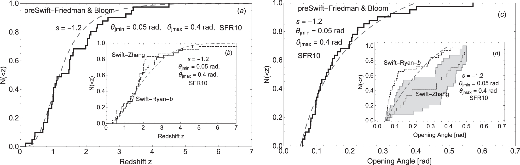
Zoom In Zoom Out Reset image size

Moving toward a more complete redshift Swift sample, we search for a GRB burst rate functional form that could fit only the Swift-Ryan-2012 redshift while predicting (1) the jet opening angle distribution for the Swift-Ryan-2012 sample and (2) the redshift and jet opening angle distributions for the pre-Swift sample. Interestingly, the calculated redshift distribution using SFR9 fits well the observed estimated Swift-Ryan-2012 redshift distribution above a redshift of 2 but is way off below it (see Figure 7(a)), while the calculated jet opening angle distribution from our model is within the Swift-Ryan-2012 statistical error bars (see Figure 7(c)). The result of the fit to the redshift distribution suggests that we have an excess of GRBs at low redshift using SFR9. This means to fit the Swift-Ryan-2012 redshift distribution we have to increase the GRB rate at lower redshift, and by doing so we shift the distribution to lower redshift, and consequently, we also shift the distribution more to the left at higher z. To finally fit the Swift-Ryan-2012 redshift distribution, we have to decrease the maximum jet opening angle to ${\theta }_{{\rm{j}},\max }=0.4\,\mathrm{rad}$, which is still within the acceptable range for LGRBs. The best-fit parameters have the range of jet opening angles between ${\theta }_{{\rm{j}},\min }=0.05\,\mathrm{rad}$ and ${\theta }_{{\rm{j}},\max }=0.4\,\mathrm{rad}$, the jet opening angle power-law index $s=-1.2$, and the γ-ray energy released ${{ \mathcal E }}_{* \gamma }=2\times {10}^{51}\,\mathrm{erg}$. These results are shown in Figures 7(b) and (c), and the fits indicate an acceptable fit to the Swift-Ryan 2012 redshift and jet opening angle distributions using SFR10 (using Equation (18) with $\alpha =8,\beta =-0.4,\gamma =-5.1,{z}_{1}=0.5,{z}_{2}=4.5;$ see Figure 1(b)). Using SFR10 we also obtain acceptable fits to the pre-Swift sample, as shown in Figures 8(a) and (c). The fitted parameters also give acceptable fits to the Swift-Zhang and Swift-Ryan-b redshift distributions and are within the estimated jet opening angle distributions between the Swift-Zhang and Swift-Ryan-b samples. For the first time, we have shown self-consistently that the GRB formation rate does follow the observed SFR, similar to the Hopkins & Beacom (2006) star formation history and as extended by Li (2008; SFR7), consistent with, for example, the Wanderman & Piran (2010), Dado & Dar (2014), Greiner et al. (2015), Sun et al. (2015), and Perley et al. (2016) analyses.

Zoom In Zoom Out Reset image size

Zoom In Zoom Out Reset image size

The SFR10 functional form, however, indicates that the GRB burst rate is higher than the observed SFR7 at all redshifts, suggesting the possibility that the burst rate could be affected by luminosity evolution with redshift (e.g., Salvaterra & Chincarini 2007; Salvaterra et al. 2009, 2012; Deng et al. 2016; Perley et al. 2016). On the other hand, the SFR9 functional form indicates that, between redshift 0.5 and 3, the GRB burst rate is lower than the observed SFR7, indicating an excess of GRBs at lower redshifts (see Figure 7(a)) and therefore suggesting the possibility that the burst rate could be affected by different progenitor populations or GRB properties, for example, due to the increasing metallicities with decreasing redshift (e.g., Fruchter et al. 2006; Berger et al. 2007). Interestingly, this excess of GRBs at low redshift is also consistent with, for example, the Yu et al. (2015) and Petrosian et al. (2015) findings. However, an interesting point to note is that in our GRB model we use a single-average value of gamma-ray energy released, ${{ \mathcal E }}_{* \gamma }=2\times {10}^{51}\,\mathrm{erg}$, to represent the gamma-ray energy released by all LGRBs. Since the observed estimated energy release in the GRB explosions is between ${10}^{48}\,\mathrm{and}\,{10}^{52}\,\mathrm{erg}$ (e.g., Friedman & Bloom 2005; Kumar & Zhang 2015), if we relax our gamma-ray energy released restriction by considering a distribution of ${{ \mathcal E }}_{* \gamma }$ over redshift or jet opening angle (e.g., Kocevski & Butler 2008; Cenko et al. 2010; Kumar & Zhang 2015) that also includes the luminosity functions that permit a potentially large number of low-luminosity events, where GRBs at higher redshift are brighter than those at lower redshift (e.g., Salvaterra et al. 2012; Deng et al. 2016), then this might improve our fits to the pre-Swift and Swift redshift and jet opening angle distributions while reducing the GRB formation density rate (SFR10 case) over all redshifts or increasing the GRB formation density rate (SFR9 case) at low redshift to match the observed star formation density rate that is similar to the SFR7 from Hopkins & Beacom (2006) and as extended by Li (2008). We plan to explore this idea in a future paper.

More importantly, in Figures 5(d) and 7(c), our model predictions for the Swift jet opening angle distributions are within the error bars estimated by Zhang et al. (2015) and Ryan et al. (2015) from the subset and complete Swift samples, respectively. However, the median jet opening angles obtained by Zhang et al. (2015) and Ryan et al. (2015) are anywhere in the range $\langle {\theta }_{{\rm{j}}}\rangle \sim [0.1\mbox{--}0.35]$ rad, indicating problems with estimating the jet opening angles from the Swift data by combining the late-time Chandra data with well-sampled Swift/XRT light curve observations (e.g., Liang et al. 2008). In fact, Wang et al. (2015) have systematically looked into the consistency between optical and X-ray afterglows, and they find that the final sample that consists of the same jet break with achromatic break times is small for the "bright" sample of GRBs.

Our model parameters suggest that GRBs can be detected with Swift to a maximum redshift $z\approx 18$. The models, SFR9 and SFR10, that fit the data imply that about 10% of Swift GRBs occur at $z\gtrsim 4$, in accord with the data shown in Figures 7(a) and (b). Our model also predicts that about 5% of GRBs should be detected from $z\geqslant 5$. If more than 5% of GRBs with $z\gt 5$ are detected by the time $\approx 100$ Swift GRBs with measured redshifts are found, then we may conclude that the GRB formation rate power-law index γ (see Equation (18)) is shallower than our fitted value $\gamma =-5.1$ above $z\approx 4.5$. By contrast, if a few $z\gtrsim 5$ GRBs have been detected, then this would be in accord with our model and would support the conjecture that the LGRB burst rate follows the SFR that is similar to the Hopkins & Beacom (2006) and extended by Li (2008) SFR history. Moreover, the models also indicate that less than 10% (20%) of LGRBs should be detected at $z\lesssim 1$ for SFR9 (SFR10), respectively. After examining the GRB samples¹ between 2013 and 2015, we notice that less than $5 \%$ of LGRBs per year were detected by Swift above $z\gt 5$, and about $\sim 10 \%$ of LGRBs were detected above $z\gt 4$, consistent with both model predictions. However, about 6% of LGRBs per year were detected below $z\lt 1$, consistent more with model SFR9.

We also compare our model size distribution with the BATSE 4B Catalog size distribution. The BATSE 4B Catalog contains 1292 bursts in total, including short- and long-duration GRBs. There are a total of 872 LGRBs that are identifiable in the BATSE 4B Catalog (Paciesas et al. 1999; Le & Dermer 2009) with a BATSE detection rate of $\approx 550$ GRBs per year over the full sky brighter than 0.3 photons ${\mathrm{cm}}^{-2}\,{{\rm{s}}}^{-1}$ in the 50–300 keV band (Band 2002). Since there are only 872 LGRBs in the catalog, the BATSE detection rate is $\approx 371$ LGRBs per year over the full sky. Figure 9(a) shows the model integral size distribution (see Equation (9)) of LGRBs predicted by our best-fit models, SFR9 and SFR10. The plots are normalized to the current total number of observed LGRBs per year from BATSE, which is 371 bursts per $4\pi$ sr exceeding a peak flux of 0.3 photons ${\mathrm{cm}}^{-2}\ {{\rm{s}}}^{-1}$ in the ${\rm{\Delta }}E=50\mbox{--}300\,\mathrm{keV}$ band for the ${\rm{\Delta }}t=1.024\,{\rm{s}}$ trigger time. From the model size distribution, we find that $\cong 235(270)$ LGRBs per year should be detected with a BATSE-type detector over the full sky above an energy flux threshold of $\sim {10}^{-7}\,\mathrm{erg}\,{\mathrm{cm}}^{-2}\,{{\rm{s}}}^{-1}$, or photon number threshold of $\gt 0.633\,\mathrm{ph}\,{\mathrm{cm}}^{-2}\,{{\rm{s}}}^{-1}$ using SFR9 (SFR10), respectively. We also estimate from our fits that $\cong 800(530)$ LGRBs take place per year per $4\pi$ sr with a flux $\gtrsim {10}^{-8}\,\mathrm{erg}\,{\mathrm{cm}}^{-2}\,{{\rm{s}}}^{-1}$, or $\gt 0.0633\,\mathrm{ph}\,{\mathrm{cm}}^{-2}\,{{\rm{s}}}^{-1}$. The field of view of the BAT instrument on Swift is 1.4 sr (Gehrels et al. 2004), implying that Swift should detect $\cong 90(60)$ LGRBs per year for SFR9 (SFR10), respectively. Currently, Swift observes about 135 GRBs per year, and applying the ratio 872/1292, we obtain $\cong 90$ LGRBs per year; this is consistent with the SFR9 model prediction.

Zoom In Zoom Out Reset image size

Finally, we show the differential size distribution of BATSE GRBs from the Fourth BATSE catalog (Paciesas et al. 1999) in comparison with our model prediction in Figure 9(b). As can be seen, our model parameters, using SFR9, give an excellent fit to the BATSE LGRB size distribution, while SFR10 overpredicts the differential burst rate above $1.0\,\mathrm{ph}\,{\mathrm{cm}}^{-2}\,{{\rm{s}}}^{-1}$. It is important to note that the size distribution of the BATSE RGB distribution in Figure 9(b) is normalized and corrected to 371 LGRBs above a photon number threshold of $0.3\,\mathrm{ph}\,{\mathrm{cm}}^{-2}\,{{\rm{s}}}^{-1}$. Below a photon number threshold of $0.3\,\mathrm{ph}\,{\mathrm{cm}}^{-2}\,{{\rm{s}}}^{-1}$ in the 50–300 keV band, the observed number of GRBs falls rapidly due to the sharp decline in the BATSE trigger efficiency at these photon fluxes (see Paciesas et al. 1999), while the size distribution of the Swift GRBs will extend to much lower values $\cong 0.0633\,\mathrm{ph}\,{\mathrm{cm}}^{-2}\,{{\rm{s}}}^{-1}$.