


Abstract
The solar wind measured in situ by Parker Solar Probe in the very inner heliosphere is studied in combination with the remote-sensing observation of the coronal source region provided by the METIS coronagraph aboard Solar Orbiter. The coronal outflows observed near the ecliptic by Metis on 2021 January 17 at 16:30 UT, between 3.5 and 6.3 R⊙ above the eastern solar limb, can be associated with the streams sampled by PSP at 0.11 and 0.26 au from the Sun, in two time intervals almost 5 days apart. The two plasma flows come from two distinct source regions, characterized by different magnetic field polarity and intensity at the coronal base. It follows that both the global and local properties of the two streams are different. Specifically, the solar wind emanating from the stronger magnetic field region has a lower bulk flux density, as expected, and is in a state of well-developed Alfvénic turbulence, with low intermittency. This is interpreted in terms of slab turbulence in the context of nearly incompressible magnetohydrodynamics. Conversely, the highly intermittent and poorly developed turbulent behavior of the solar wind from the weaker magnetic field region is presumably due to large magnetic deflections most likely attributed to the presence of switchbacks of interchange reconnection origin.
Export citation and abstract BibTeX RIS

Original content from this work may be used under the terms of the Creative Commons Attribution 4.0 licence. Any further distribution of this work must maintain attribution to the author(s) and the title of the work, journal citation and DOI.
1. Introduction
One of the most important and long-standing objectives of solar and heliospheric physics is to magnetically connect the solar wind streams observed in situ to their solar sources. For this purpose, different approaches have been adopted and are mainly classified into two main classes: backward ballistic mappings starting from in situ measurements at Earth, and forward modeling based on remote-sensing observations of the Sun.
Backward reconstructions (Schatten et al. 1968; Wilcox 1968) consist of a ballistic extrapolation of solar wind measurements back to the outer corona, combined with a further projection down to the photosphere, assuming that the coronal flows follow the magnetic field line topology (Neugebauer et al. 1998). Ballistic mapping assumes stationary flow from the upper corona to Earth (Krieger et al. 1973) and therefore does not account for the complex dynamical processes that occur during solar wind evolution throughout the heliosphere, such as the formation of stream interaction regions (e.g., Burlaga 1974) or the propagation of transient events into interplanetary space (e.g., Dryer 1974; Klein & Burlaga 1982). Global models, like the potential field source surface (PFSS) extrapolation (originally proposed by Altschuler & Newkirk 1969; Schatten et al. 1969), are employed to derive the coronal magnetic field channeling plasma flows from the photosphere to the source surface (whose altitude above the Sun is generally set at 2.5 R⊙; Altschuler & Newkirk 1969), above which the coronal plasma is assumed to expand radially. Specifically, the coronal magnetic field configuration is reconstructed by applying an evolving surface flux transport model to observations of the photospheric magnetic field, which act as inner boundary conditions. Although the PFSS fails in depicting solar eruptions occurring only under nonpotential field configurations, it is a widely used approach to provide an estimate of the coronal magnetic field topology. In particular, it succeeds in describing the position of the open- and closed-field regions, as well as the neutral line, which separates areas of opposite magnetic polarity (Nitta et al. 2006; Mandrini et al. 2014). Recently, Panasenco et al. (2020), based on Parker Solar Probe (PSP; Fox et al. 2016) measurements of the pristine solar wind in the very inner heliosphere, refined the PFSS model by relaxing assumptions about geometry and location of the source surface, which was indeed shown to have a nonspherical boundary and, in some cases, a lower height than the traditional 2.5 R⊙.
Within the second category is the forward modeling of magnetic fields in the corona from photospheric measurements, followed by the transport of coronal plasma (frozen in magnetic field) into interplanetary space. This approach makes use of the PFSS extrapolation, generally coupled with the Schatten Current Sheet (SCS) model (Schatten 1971) to derive the large-scale coronal magnetic field. Heliospheric propagation models, such as the Wang–Sheeley–Arge (WSA; Wang & Sheeley 1990; Sheeley & Wang 1991; Arge & Pizzo 2000) or the Heliospheric Upwind eXtrapolation (HUX; Riley & Lionello 2011; Owens et al. 2017; Reiss et al. 2019, 2020) model, are then employed to deduce the solar wind conditions near the Sun and evolve them throughout the heliosphere. The WSA coronal model is furthermore customarily used as input to initiate magnetohydrodynamic (MHD) numerical simulations of the 3D heliospheric structure and evolution of the solar wind from Sun to Earth. The MHD models currently used for operational space weather predictions are the well-known Enlil (Odstrcil 2003) and the EUropean Heliospheric FORecasting Information Asset (EUHFORIA; Pomoell & Poedts 2018). The interested reader is referred to Rouillard et al. (2020), where the current tools and techniques for modeling the Sun, its atmosphere, and the solar wind are comprehensively reviewed within the context of supporting remote-sensing and in situ observations of current and future solar missions. Worth mentioning is finally the new and very promising method proposed by Biondo et al. (2021) for simulating the Parker spiral solar wind, called the Reverse In situ data and MHD APproach (RIMAP). What makes RIMAP different from the above tools is its "dual" nature. By combining a backward ballistic reconstruction (according to the steady-state solar wind flow model by Weber & Davis 1967) of the plasma properties at 0.1 au with a successive forward propagation of the solar wind from the so-inferred boundary conditions (via PLUTO-based MHD numerical simulations; Mignone et al. 2007, 2012), RIMAP lies conceptually in between the above two categories, thus being less affected by the limitations of each class, while at the same time exploiting their respective strengths.
Successful determinations of the solar wind connectivity in conjunction with joint in situ and remote-sensing observations enable investigations of some of the most outstanding science questions in heliophysics. These include, for instance, the links and interplay between local (microscopic) and global (macroscopic) processes in the solar wind. This is particularly relevant for the quadrature configuration of two spacecraft with respect to the Sun, where the plasma locally sampled with in situ instruments is observed also remotely with coronagraphs and/or heliospheric imagers. It is worth noting, however, that not all quadratures are useful. Indeed, if the vantage points of both spacecraft are close to Earth's orbit or beyond, it is extremely difficult to succeed in identifying the magnetic connection with the solar source, either because the plasma has been reprocessed during its expansion or because of the occurrence of stream–stream interactions during propagation, both of which pose serious limitations to these kinds of investigations. The advent of PSP and Solar Orbiter (SO; Müller et al. 2020), both orbiting within the inner heliosphere, could make this task easier. A close quadrature, or rather a remote observation of the solar corona up to a few solar radii (about ten) and a local (i.e., in situ) measurement of the plasma within 0.1–0.2 au, would be indeed optimal. Telloni et al. (2021a) studied the first SO–PSP quadrature, which occurred in 2021 mid-January, focusing on tracking the same plasma parcel propagating from the corona, imaged with the Metis coronagraph (Antonucci et al. 2020), to PSP. Another approach, which is explored in the present study, is to connect solar wind measured by PSP with coronal observations provided by Metis without the need to study the same plasma parcel, but rather the one coming from the same source region, i.e., the same stream. The aim of this work is thus to make use of coordinated remote and local measurements to link the small-scale properties of the solar wind sampled by PSP to the large-scale features of the coronal source regions observed by Metis on board SO, exploiting the first quadrature Metis/SO–PSP. The text is organized as follows: methodological approach to the analysis of PSP and SO data (Section 2), presentation (Section 3) and interpretation of the results (Section 4), and conclusions (Section 5).
2. Orbital Geometry and Connectivity
The approach followed in this work takes advantage of the orbital motion of PSP. When approaching perihelion, PSP has a longitudinal speed higher than that of the solar rotation. Then, as it moves away from the Sun, PSP slows down, initially corotating with the Sun and finally traveling with a longitudinal speed lower than the rotating solar surface. This property of the PSP orbits offers great opportunities to study the evolution of solar wind turbulence. Indeed, as PSP moves back-and-forth in longitude with respect to the Sun, the spacecraft may sample solar wind streams coming from the same source region at the Sun twice. This scenario, first exploited by Shi et al. (2021), is sketched in Figure 1. Assuming a rigid rotation of the solar corona (e.g., Antonucci & Svalgaard 1974; Giordano & Mancuso 2008), PSP crossed the plane of the sky (POS) observed by the coronagraph Metis on 2021 January 17 at 16:30 UT (t0 in Figure 1) and on 2021 January 18 at 18:59 UT (t1), when PSP was at 0.11 au. Later during encounter 7, on 2021 January 23 at 17:02 UT (t3), while leaving the perihelion passage at a distance of 0.26 au, PSP was passed again by the plane corresponding to the longitude observed by Metis.
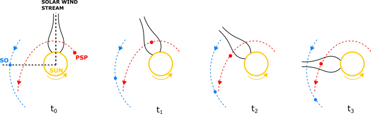
Figure 1. Cartoon representation of the PSP's double crossing (at instants t1 and t3) of the POS observed by Metis (at instant t0), marked by the vertical black dashed line. The generic instant t2 refers to an intermediate configuration between t1 and t3, when PSP, moving at a speed greater than that of the solar rotation, initially passed the Metis POS. The positions of SO and PSP at different instants along their trajectories (blue and red dashed curves) are shown as blue and red filled circles, respectively.
Download figure:
Standard image High-resolution imageThese instants have been obtained by equating the longitude of PSP's orbit (red line in Figure 2(a)) with that observed at the east limb by Metis at t0 (λ = 99°, filled orange circle, that is, the longitude of SO at t0, filled blue circle, decreased by 90° to take into account that the Metis POS is perpendicular to the Sun–SO line) and increasing at the rate of 14 7 day–1 (i.e., assuming a sidereal solar rotation period of 24.47 days at the equator) as the Sun rotates eastward (orange curve in Figure 2(a)).

Figure 2. HCI (a) longitude and (b) latitude of SO (blue), PSP (red), and the Metis POS at the east limb (orange) during the spacecraft trajectories around the Sun (yellow star), displayed in the (c) side and (d) top views of the equatorial plane, from 2021 January 17 to 24. Blue and orange filled circles correspond to time t0, while open and filled red circles refer to the two crossings of the Metis POS by PSP at t1 and t3. The SO–Sun line and the eastern limb of the Metis POS at t0 are also marked as dotted lines in the X-Y plane (panel (d)).
Download figure:
Standard image High-resolution imageThe positions of PSP at t1 and t3 (open and filled red circles, respectively) and that of SO at t0 (filled blue circle) in the X-Z and X-Y planes of the HelioCentric Inertial (HCI) coordinate frame are displayed, along with their orbits from 2021 January 17 to 24, in Figures 2(c) and (d), respectively. The longitude at the east limb corresponding to the Metis POS is marked as a dotted line in the top view of the equatorial plane (Figure 2(d)). Applying a tolerance of ±1° in longitude, two time intervals (samples #1 and #2) of 2.4 and 5.5 hr centered approximately on the above times, t1 and t3, are thus identified as corresponding to the same longitude observed by Metis at the east limb at t0. It is worth noting that the second interval is longer than the first because during the second crossing the longitudinal speed of PSP was closer to the Sun's sidereal rotation than it was during the first.
However, during its motion from t1 to t3, PSP moved, albeit slightly, in latitude, from just above to just below the equatorial plane (red curve in Figure 2(b)), crossing the quite warped heliospheric current sheet (HCS). This is clearly evidenced by the sharp magnetic field ∼180° rotation measured by PSP late on 2021 January 19 (as shown below). It follows that, although corresponding to the same longitude, PSP measurements at t1 and t3 correspond to two solar wind streams coming from regions on opposite sides of the neutral line on the solar surface, i.e., from two different coronal sources with opposite polarities. Further evidence thereof comes by establishing the coronal origins of the solar wind observed by PSP during the selected time periods. This is accomplished by projecting the PSP spacecraft positions onto the PFSS surface, according to the mapping procedure developed by Panasenco et al. (2020): as clearly shown in Figure 3, on 2021 January 18 and 23 PSP (in blue) was connected to two different source regions, in fact below and above the neutral line. Specifically, although magnetically connected at approximately the same Carrington longitude observed by Metis at t0 (vertical dashed line), on 2021 January 18 at 17:49–20:12 UT (sample #1) PSP sampled a stream coming from the equatorial extension of the southern polar hole, characterized by a strong magnetic field. Conversely, on 2021 January 23 at 04:17–19:45 UT (sample #2), PSP was crossed by solar wind plasma emitted from the extension at low latitudes of a northern coronal hole and connected to a weaker magnetic field region with opposite (positive) polarity.

Figure 3. Projections of PSP's positions on 2021 January 18 and 23 onto the source surface (blue crosses) and down to the solar wind source region (blue circles), located at 2.0 and 1.2 R⊙, respectively. Open-field regions with positive (green) and negative (azure) magnetic polarity in the PFSS ∣ B ∣2 contour map are separated by the neutral line (thick black curve). Horizontal red and blue dashed lines refer to the PSP's heliographic latitude at t1 and t3. The vertical black dashed line marks the (Carrington) longitude of the Metis POS at t0.
Download figure:
Standard image High-resolution image3. Remote-sensing and In Situ Observations
3.1. Metis Data
The polarized brightness (pB) and the H i Lyα ultraviolet (UV) emission observed by Metis at t0 are imaged in Figures 4(a) and (b), respectively (see Antonucci et al. 2020, for a complete description of the Metis polarimetric and UV channels).

Figure 4. Overview of the Metis data analysis, showing the (a) pB and (b) UV H i Lyα images acquired on 2021 January 17 at 16:30 UT (t0) and the radial profiles at latitudes of −35 (red triangles) and 045 (blue triangles) of (c) pB, (d) UV intensity, (e) electron density, (f) radial outflow velocity, and (g) density flux.
Download figure:
Standard image High-resolution imageDuring the Metis observations, SO was at a distance of 0.58 au from the Sun, so the 16–29 annular field of view (FOV) of Metis extended from 3.5 to 6.3 R⊙ above the solar limb. Latitudes of −35 and 05 with respect to the equatorial plane pointing to PSP positions at t1 and t3 are marked as a red and blue line, respectively. At these latitudes, the Metis observations therefore provide information on the large-scale physical properties and dynamics (i.e., electron density and outflow velocity) of the streams later locally sampled by PSP during its two successive crossings of the Metis POS. The relative pB and UV intensity radial profiles (obtained by averaging Metis observations over 2°-wide angular sectors centered on the corresponding latitudes and in steps of 0.1 R⊙) are shown in Figures 4(c) and (d), respectively. From these are then inferred the radial profiles of the electron density ne
(Figure 4(e)) and radial outflow velocity VR
(Figure 4(f)) of the coronal flows measured by PSP at t1 and t3. The reader is referred to Antonucci et al. (2020) for a fairly comprehensive description of the diagnostic techniques to be applied to Metis data in order to derive these coronal quantities. It is worth mentioning here that ne
and VR
are derived by making use of the van de Hulst inversion (van de Hulst 1950) and Doppler dimming (Noci et al. 1987) techniques, respectively. In doing so, some parameters measured by PSP (i.e., the proton temperature Tp
and density np
, and the proton temperature anisotropy T⊥,p
/T∥,p
) in the corresponding samples #1 and #2, properly scaled to coronal heights (e.g., Perrone et al. 2019), were employed in the calculations. The other coronal parameters involved in deriving VR
(such as helium abundance and electron temperature) were assumed as in Telloni et al. (2021a). Finally, the particle flow rate per unit area, i.e., the density flux ne
VR
, is displayed in Figure 4(g).
3.2. PSP Data
Figure 5 presents an overview of the PSP plasma and magnetic field measurements acquired, respectively, with the SWEAP (Kasper et al. 2016) and FIELDS (Bale et al. 2016) instruments, during encounter 7 from 2021 January 17 to 24. Samples #1 and #2 are indicated by the two pairs of vertical dashed lines. Corresponding average values are reported in Table 1.

Figure 5. Overview of the PSP measurements during encounter 7, encompassing the intervals #1 and #2 of interest (located between dashed vertical lines). The panels show, from top to bottom, the R-component of the plasma
V
and Alfvén
V
A velocity, the magnetic field radial component (BR
) and magnitude (B), the angles between
B
and  (θRB) and
V
(θVB), the proton number density np
, temperature Tp
, temperature anisotropy T⊥,p
/T∥,p
, plasma beta βp
, and the altitude of PSP above the Sun.
(θRB) and
V
(θVB), the proton number density np
, temperature Tp
, temperature anisotropy T⊥,p
/T∥,p
, plasma beta βp
, and the altitude of PSP above the Sun.
Download figure:
Standard image High-resolution imageTable 1. Average Values of the PSP Solar Wind Parameters in the Two Time Intervals #1 and #2 under Study
| Parameters | #1 | #2 |
|---|---|---|
| (red) | (blue) | |
| VR (km s−1) | 218 | 291 |
| VA,R (km s−1) | 50 | 16 |
| B (nT) | 203 | 21 |
| BR (nT) | −144 | 17 |
| θRB (deg) | 140 | 38 |
| θVB (deg) | 129 | 39 |
| np (cm−3) | 4.54 × 10³ | 5.45 × 10² |
| Tp (K) | 4.57 × 10⁵ | 3.16 × 10⁵ |
| T⊥,p /T∥,p | 0.97 | 0.81 |
| βp | 3.5 | 45.8 |
| r (au) | 0.11 | 0.26 |
Download table as: ASCIITypeset image
From top to bottom are the radial component of the plasma
V
and Alfvén VA ( , where μ0,
B
, and ρ are the vacuum magnetic permeability, the magnetic field vector, and the mass density, respectively) velocity, the magnetic field radial component (BR
) and intensity (B) in the Radial Tangential Normal (RTN) coordinate system, the angles of the magnetic field vector with respect to the radial direction θRB and the flow velocity θVB, the proton number density, temperature, temperature anisotropy, plasma beta βp
( ≡ P/(B2/2(μ0)), i.e., the ratio between the plasma P = np
kB
Tp
, with kB being the Boltzmann constant, and magnetic pressures), and the distance of PSP from the Sun. As mentioned above, the magnetic field is in the sunward (outward) direction, i.e., BR
≶ 0 and θRB ∼ 180° (0°) (Figures 5(b) and (c)), in sample #1 (#2), thus confirming PFSS predictions of Figure 3: the two coronal flows emerge from below and above the neutral line, respectively, and are therefore sampled by PSP from opposite sides of the HCS.
, where μ0,
B
, and ρ are the vacuum magnetic permeability, the magnetic field vector, and the mass density, respectively) velocity, the magnetic field radial component (BR
) and intensity (B) in the Radial Tangential Normal (RTN) coordinate system, the angles of the magnetic field vector with respect to the radial direction θRB and the flow velocity θVB, the proton number density, temperature, temperature anisotropy, plasma beta βp
( ≡ P/(B2/2(μ0)), i.e., the ratio between the plasma P = np
kB
Tp
, with kB being the Boltzmann constant, and magnetic pressures), and the distance of PSP from the Sun. As mentioned above, the magnetic field is in the sunward (outward) direction, i.e., BR
≶ 0 and θRB ∼ 180° (0°) (Figures 5(b) and (c)), in sample #1 (#2), thus confirming PFSS predictions of Figure 3: the two coronal flows emerge from below and above the neutral line, respectively, and are therefore sampled by PSP from opposite sides of the HCS.
3.3. Solar Wind Large-scale Properties
Focusing first on the large-scale features of the two streams, the one emanating from the north polar hole extension with a weaker magnetic field at the coronal base (which ensures a larger plasma beta, as observed, see Figure 5(g)) is denser (Figure 4(e)) and expands in both the corona (Figure 4(f)) and heliosphere (Figure 5(a)) at a higher speed compared to that originating in the southern stronger field region. That is, the particle flux density ne VR is larger for a weaker magnetic field in the coronal source region (Figure 4(g)). Assuming that the magnetic field is frozen into the fluid and relying on conservation of mass and magnetic flux, the observed relationship between the coronal particle flux and the magnetic field at the base of the corona follows from similar results found by Wang (1995) at the top of the chromospheric−transition region boundary. This is furthermore in accordance with predictions from turbulence transport and heating models tied to an explicit solar wind model aimed at providing bulk parameters (see the review by Zank et al. 2021, and references therein): in these models, ne VR in the corona is inversely proportional to the magnetic field strength at the base of the corona. Both coronal flows undergo a more significant acceleration at heliocentric distances below ∼4 R⊙ and then reach a fairly steady rate, as appears evident from the near-linear velocity profiles for r ≳ 4 R⊙ (Figure 4(f)). However, while the flow from below the neutral line (sample #1; red triangles) appears to have reached a steady-state velocity at the outer edge of the Metis FOV (the velocities at PSP and coronal heights are indeed very similar), the flow from above the neutral line (sample #2; blue triangles) should experience some residual acceleration up to the PSP position, since the velocity measured by PSP is about 30% larger than that inferred at 6.3 R⊙. Thus, it might be argued that an additional energy deposition mechanism may be at work, between 6.3 R⊙ and 0.1 au, in the plasma of stream #2, to accelerate it to higher velocities. Looking at the PSP data, a visual inspection (Figure 5) suggests that the time profiles of sample #1 are relatively smoother than those of sample #2, which instead appears to be characterized by more velocity spikes, indicating accelerated wind bursts, larger and sharper magnetic field deflections (not reversing the field direction, though), and stronger density fluctuations. While it is clear that a spectral analysis (performed below) is needed to corroborate these insights, even this first glimpse of the PSP data suggests how the differences in the two coronal source regions from which the two streams originate affect the local properties of the solar wind plasma.
3.4. Solar Wind Small-scale Properties
Focusing now in detail on the small-scale properties of the two streams under study, Figure 6 presents a standard analysis of the turbulence properties of solar wind fluctuations (Bruno & Carbone 2013) in the selected PSP time intervals. Specifically, Figures 6(a)–(d) display (in red and blue, for samples #1 and #2, respectively) the spectra of the magnetic field vector fluctuations δ
B
2, magnetic compressibility C = δ
B2/δ
B
2 (i.e., the ratio between the powers associated with magnitude fluctuations δ
B2 and with vector fluctuations δ
B
2, which is in any case smaller than 1, since δ
B
2 ≥ δ
B2), flatness  (i.e., the ratio between the fourth and the squared second-order structure functions of the magnetic field vector increments Δ
B
), and normalized cross-helicity σc
( ≡ 2
u
·
b
/(〈u2〉 + 〈b2〉) = (e+ − e−)/(e+ + e−), i.e., a customary measure of the alignment between magnetic
(i.e., the ratio between the fourth and the squared second-order structure functions of the magnetic field vector increments Δ
B
), and normalized cross-helicity σc
( ≡ 2
u
·
b
/(〈u2〉 + 〈b2〉) = (e+ − e−)/(e+ + e−), i.e., a customary measure of the alignment between magnetic  and velocity
u
fluctuating field vectors, say, Alfvénicity, or, alternatively, of the imbalance between forward (e+) and backward (e−) Alfvén mode energies).
and velocity
u
fluctuating field vectors, say, Alfvénicity, or, alternatively, of the imbalance between forward (e+) and backward (e−) Alfvén mode energies).

Figure 6. Spectra of (a) the magnetic field trace power δ
B
2, (b) magnetic compressibility C, (c) flatness  , and (d) normalized cross-helicity σc
and (e) Politano-Pouquet linear scaling, for samples #1 (red) and #2 (blue). Power-law fits at fluid and sub-ion scales are shown as color-coded lines in panels (a) and (c), along with the corresponding spectral scalings, α and β. The linear fit in the inertial range (black line) is indicated in panel (e), where the mean energy transfer rate, ε, is also reported. Positive (negative) values in panel (e) are indicated by filled (open) symbols.
, and (d) normalized cross-helicity σc
and (e) Politano-Pouquet linear scaling, for samples #1 (red) and #2 (blue). Power-law fits at fluid and sub-ion scales are shown as color-coded lines in panels (a) and (c), along with the corresponding spectral scalings, α and β. The linear fit in the inertial range (black line) is indicated in panel (e), where the mean energy transfer rate, ε, is also reported. Positive (negative) values in panel (e) are indicated by filled (open) symbols.
Download figure:
Standard image High-resolution image
For frequencies in the spacecraft frame below 0.1 Hz (i.e., in the inertial range of turbulence), the large normalized cross-helicity (0.6 ≲ σc ≲ 0.9; Figure 6(d)) and very low magnetic compressibility (C ∼ 10−3; Figure 6(b)) suggest the Alfvénic nature of the magnetic field fluctuations observed in sample #1 (in the sub-ion range, though, magnetic compressibility increases, likely due, as discussed below, to the presence of intermittent structures emerging at smaller scales from the sea of lower-amplitude Alfvénic fluctuations). In the same range of scales, the spectral power trace displays a standard power-law scaling with exponent close to 3/2 (as inferred by fitting fluid scales between 10−3 and 10−1 Hz; black line in Figure 6(a)), typical of Alfvénic turbulence. An Iroshnikov−Kraichnan-like (IK) spectrum (Iroshnikov 1963; Kraichnan 1965) of the magnetic fluctuations has been widely observed by PSP close to the Sun (e.g., Chen et al. 2020; Telloni et al. 2021b; Zhao et al. 2022a). Such a value of the spectral exponent is observed, in the present analysis, in a field-aligned flow (θVB ∼ 180°; Figure 5(c)), thus incidentally preventing the sampling of advected quasi-2D structures; it follows that slab fluctuations are mostly observed (Zank et al. 2020b), as discussed in more detail below. Additionally, the interval shows a standard level of inertial range intermittency (e.g., Bruno et al. 2003) and enhanced intermittency in the kinetic range (Alexandrova et al. 2008), as measured through the fast power-law increase of the flatness (with scaling exponents β = 0.37 and β = 0.42), a widely adopted descriptor for assessing deviation from Gaussian distributions of solar wind fluctuations (e.g., Dudok de Wit et al. 2013; Sorriso-Valvo et al. 2021). According to previous work reported in the literature (e.g., Telloni et al. 2019; Zhao et al. 2020), the above observations do not support the critical balance prediction of steeper and weakly intermittent turbulence for fluctuations sampled parallel to the magnetic field (Goldreich & Sridhar 1995).
On the other hand, sample #2 exhibits a steeper spectrum in the inertial range of scales (with exponent α = 1.71), followed by an even steeper scaling at higher frequencies at sub-ion scales (Figure 6(a)). Furthermore, unlike the first stream, the second is characterized by highly compressive magnetic fluctuations (as indicated by C ≳ 0.1 and σc ≲ 0.4 within the whole range of frequencies, Figures 6(b) and (d)), which are therefore not (or, at least, less) Alfvénic. Rather, those sampled are magnetic structures. This is corroborated by the faster growth of the flatness found in the second interval (Figure 6(c)), which might suggest a higher intermittency (e.g., Bruno et al. 2003), as expected in the case of coherent structures advected by a wind with a smaller content of Alfvénic fluctuations (Zank et al. 2020b). Note, however, that in sample #2 the scaling of the flatness has an evident break near 0.01 Hz, where the steep increase observed at lower frequencies becomes shallower in the core of the inertial range (0.01–1 Hz). The break appears to occur at the frequency where the normalized cross-helicity becomes negligible, but with no clear signature in the spectrum, suggesting that interval #2 is not well described by standard intermittent turbulence.
The global energy transfer across scales in the turbulent cascade is described in finer detail by a relation between the third-order moments of the incompressible MHD field fluctuations, Y(Δt) = 〈ΔvL (∣Δ v ∣2 + ∣Δ b ∣2) − 2ΔbL (Δ v · Δ b )〉, and the mean energy transfer rate, ε, known as the Politano−Pouquet (PP) law (Politano & Pouquet 1998):

where U is the bulk solar wind speed. ΔbL (ΔvL ) are the longitudinal increments of the magnetic field (plasma flow) component across a temporal lag, Δt, along the sampling direction. Brackets indicate sample average. Average values of U over the two intervals are used to transform spatial lags, ℓ, to temporal lags according to the Taylor hypothesis, ℓ = − UΔt (Taylor 1938), which is robustly verified in the samples under study. The linear scaling of the mixed third-order structure functions with timescale is valid for turbulent flows that are statistically homogeneous, stationary, at high Reynolds number (namely, showing an extended inertial range), and locally isotropic. The PP law is broadly observed in space plasmas, for incompressible MHD (Sorriso-Valvo et al. 2007; Smith et al. 2009), including Hall effects (Hellinger et al. 2018; Ferrand et al. 2019; Bandyopadhyay et al. 2021), and for compressible MHD (Hadid et al. 2018; Andrés et al. 2019; Zhao et al. 2022b), providing important information on the status of the turbulent cascade, as well as on the nonlinear contribution to the global cross-scale energy transfer.
Figure 6(e) displays the PP scaling law, given by Equation (1), for the two intervals of interest. Filled and open markers indicate positive and negative values of the third-order moment Y, respectively. In the first interval (red) a well-defined linear scaling range is evident between approximately 3.5 and 120 s, which is roughly consistent with the spectral inertial range. The linear fit of the PP law (black line) gives a mean energy transfer rate ε = 282 ± 35 kJ kg−1 s−1, indicating a strongly active, fully developed nonlinear energy turbulent cascade (from large to small scales), and which is compatible with previous observations in the inner heliosphere (Bandyopadhyay et al. 2021; Hernández et al. 2021; Sorriso-Valvo & Yordanova 2022). In the second interval (blue), albeit comparable in magnitude, the third-order moment shows an evident lack of sign convergence, with alternating positive and negative values at different scales. A consistently positive range exists at large scale, between 100 and 2000 s. However, in that range the third-order moment is nearly constant, so that the linear scaling of the PP law is not observed. This may be due to a failure of the PP law hypothesis, as for example the nonnegligible contribution of compressive effects, and is most likely evidence that the turbulent cascade is not fully developed, or that structures not generated by the turbulence nonlinear interactions are present. The latter conjecture is also confirmed by the observed double power-law scaling of the flatness.
Similar findings are obtained when considering longer intervals centered on t1 and t3 (assuming a larger tolerance of ±2° and ±4° in longitude; see Section 2), though still connected to the same source regions as the shorter samples. This ensures the statistical significance and ergodicity of the results presented in Figure 6. It is unclear whether the differences in turbulent properties described above (power-law exponent, Alfvénicity, intermittency, and scaling of the third-order moment, i.e., degree of turbulence development) for the two streams under study are due to the radial evolution of turbulence (sample #1 at 0.11 au and sample #2 at 0.26 au) as much as to different boundary/base/source region conditions (they are certainly not due to a different spacecraft sampling direction, since in both cases this is almost parallel to the magnetic field direction, θRB ∼ 180° (0°); Figure 5). However, a radial excursion of only 0.15 au appears to be too small to explain those large differences, which are therefore more likely to be attributed, as discussed in the following section, to the differences of the two coronal source regions.
4. Interpretation
This section is devoted to interpreting, at least qualitatively, results achieved in the corona and solar wind (along with PFSS predictions) as a whole in light of the theory and transport of nearly incompressible magnetohydrodynamics (NI MHD) turbulence (Zank et al. 2017).
Interpretation of sample #1 properties is more straightforward. Relevant in this regard are the angle between the magnetic field vector and the plasma flow, the normalized cross-helicity, and the strength of the magnetic field of the solar source region. Indeed, the observations are made in a highly field-aligned flow with minor deviations from the radial, so PSP is looking at waves, almost certainly Alfvén waves given the very low compressibility, and almost exclusively outwardly propagating (σc ∼ 1). As discussed above in Section 3.4, where the properties of the small-scale fluctuations in interval #1 are presented, the magnetic field parallel spectrum has a −1.57 ∼ −3/2 slope, suggesting an IK spectrum despite the Alfvénic fluctuations being almost entirely outwardly propagating (σc ∼ 1). This observation (similar to observations made by Wang et al. 2015; Telloni et al. 2019; Zhao et al. 2020) (i) cannot be explained by IK theory, which requires counterpropagating Alfvén waves (ideally with σc ∼ 0) to initiate the cascade, and (ii) cannot be explained by the Goldreich & Sridhar (1995) critical balance theory, which also needs counterpropagating waves (σc ∼ 0) and moreover predicts a parallel spectrum of −2. Even the critical balance extension to imbalanced turbulence (Lithwick et al. 2007; Chandran 2008; Beresnyak & Lazarian 2008; Perez & Boldyrev 2009) predicts a strong wavevector anisotropy, with the perpendicular spectrum dropping off as −5/3 (or −3/2, as suggested by numerical simulations by Beresnyak & Lazarian 2009; Perez & Boldyrev 2010) and the parallel spectrum scaling as −2. It follows that even the critical balance theory with nonzero cross-helicity is unable to explain the observed −1.57 magnetic field parallel spectrum. The NI MHD theory (Zank et al. 2020b) predicts, on the other hand, a parallel turbulence spectrum of − 3/2 for unidirectionally propagating Alfvén waves. The NI MHD theory is closely related to the solar wind heating model presented by Zank et al. (2018), in which the strong magnetic field environment at the coronal base generates quasi-2D fluctuations as the magnetic carpet emerges, along with a minority population of outwardly propagating Alfvén waves. The interaction of Alfvén waves and quasi-2D structures can produce the cascade even for unidirectionally propagating Alfvén waves according to the spectral theory presented by Zank et al. (2020b). The spectral observations presented here resemble in many respects the observations presented in Zank et al. (2022) and Kasper et al. (2021), both focusing on the investigation of the turbulent properties of a sub-Alfvénic interval dominated by slab/Alfvénic fluctuations.
Interpretation of results related to sample #2 is more challenging. Again the information from θVB is instructive. Although radial on average, the excursions from alignment are much larger than those exhibited by the sample #1 interval. Although a closer and more thorough look would be worthwhile to provide a more quantitative interpretation (which is beyond the scope of this paper), it certainly appears that there are some large field deflections, most likely attributed to switchbacks (e.g., Bale et al. 2019). The key difference between samples #1 and #2 might be thus the possibility of switchbacks introducing a second statistically independent component of turbulence. Indeed, it was recognized that unidirectionally propagating Alfvénic fluctuations are superimposed on and within switchbacks (e.g., McManus et al. 2020, where they introduced a different definition of cross-helicity to account for the propagation of unidirectional waves in a switchback). If switchbacks are present, the results found in sample #2 can be interpreted as follows. In their original analysis, Dudok de Wit et al. (2020) showed that there seemed to be two populations of magnetic field fluctuations: turbulence and switchbacks (which do not have to exhibit full field reversals, these belonging just to the most extreme events) that appeared to be younger and distinct from older/well-developed turbulent fluctuations. This motivated the work by Zank et al. (2020a), where switchbacks are interpreted as a consequence of interchange reconnection events, similar to Fisk & Kasper (2020) and Drake et al. (2021). However, in Zank et al. (2020a) switchbacks are argued to be fast-mode (although in a low-beta plasma this means that their phase velocity is that of Alfvén waves), large-amplitude structures (i.e., compressible), not limited to propagation in the mean field direction only. Thus, in a statistically two-component set of magnetic field fluctuations, a variety of observational evidence would be expected: (i) a superposition of two possibly independent spectra (the observed −1.71 spectral exponent might be thus interpreted as a mixture of the − 3/2 scaling typically observed by PSP close to the Sun and the −2 switchback-related spectrum); (ii) a confused cross-helicity because of the propagation of unidirectional waves in a highly fluctuating large-amplitude magnetic field environment; (iii) a higher level of compressibility because switchbacks (at least in one theoretical manifestation) are compressible; (iv) a higher level of intermittency because switchback-driven deviations from the radial direction presumably allow for the observation of quasi-2D structures (impossible in the more field-aligned interval #1), which would increase intermittency; and (v) a third-order moment without linear scaling. Furthermore, energy dissipation via switchbacks (largely not yet understood) may also explain the spectral steepening observed in interval #2 at high frequencies (if switchbacks are fast-mode structures, then dissipation may be due to wave steepening; Zank et al. 2020a), as well as the higher velocity of the relative solar wind plasma (pointing, as discussed above, to an extra energy input). Another noteworthy point is that the temperature anisotropy T⊥/T∥ is different in the #1 and #2 intervals, being nearly isotropic in sample #1 but lower in sample #2: this anisotropy would be consistent with switchback generation by interchange magnetic reconnection, since that would both introduce a reconnection-accelerated anisotropic component into the coronal plasma and release loop plasma into the fast wind (Zank et al. 2020a). Finally, from the interchange reconnection origin theory, switchbacks would likely be observed in regions close to the boundary between a coronal hole and loops with opposite magnetic polarity. Figure 3 shows indeed that the source region of the second wind stream is at the boundary between the northern polar coronal hole and a closed loop-dominated region (as indicated by the magnetic footpoints) just above the neutral line. All of this closely resembles observations related to sample #2, which can therefore be interpreted based on the presence of switchbacks in addition to turbulent fluctuations. Future work will include careful comparative theoretical and observational analysis in intervals with and without switchbacks, with the aim of supporting the aforementioned insights. This is actually the subject of a paper in preparation (G. P. Zank et al. 2022b, in preparation).
5. Conclusions and Outlook
The methodological approach described in this paper promises to be a very powerful diagnostic for linking the local properties of solar wind streams to the global features of their coronal source regions, especially in the context of future quadratures between SO and PSP. 52 In fact, in spite of being the first one, the 2021 January SO–PSP quadrature was not the most suited for this kind of investigation, since SO was not at aphelion (and thus the Metis FOV was not as wide as possible) and PSP, although approaching the Sun as close as 0.1 au, was not at the very low altitudes that it will attain during the next encounters, when the orbits will gradually shrink.
While drafting the paper, on 2022 February 23 SO, orbiting at 0.64 au, was in quadrature with both PSP and BC. These two spacecraft were therefore radially aligned above the east limb of the Sun, as seen from SO, at distances of 0.12 au (PSP) and 0.32 au (BC). The Metis FOV extended from 3.8 to 6.9 R⊙. In addition, since the quadrature was at the east limb, observations from the Solar Orbiter Heliospheric Imager (SoloHI; Howard et al. 2020) complemented those of Metis, extending the range of observed heliocentric distances from 12.9 R⊙ up to 0.64 au. The SoloHI FOV in fact encompassed both PSP and BC, thus remotely observing the plasma sampled locally by the two probes. This is a unique orbital configuration, which offers a very promising opportunity to study the origin and propagation of the coronal plasma in the inner heliosphere. Indeed, the coordinated measurements from imagers aboard SO and in situ instrumentation aboard PSP and BC will make possible a deep investigation of the physical properties of the expanding solar wind plasma. Moreover, during this quadrature, the Large Angle Spectrometric Coronagraph (LASCO; Brueckner et al. 1995) aboard the SOlar and Heliospheric Observatory (SOHO; Domingo et al. 1995) and the coronagraph package of the Sun-Earth Connection Coronal and Heliospheric Investigation (SECCHI; Howard et al. 2008) instrument suite aboard the ahead spacecraft of the Solar TErrestrial RElations Observatory (STEREO; Kaiser et al. 2008) imaged the solar corona from two different points of view (their longitudinal separations from SO were 14° and −21°, respectively). This allows an interesting stereoscopic reconstruction of the solar corona crossed by PSP during its perihelion passage along orbit 11.
An even more interesting orbital configuration, which will maximize the scientific return of SO and PSP observations, will occur on 2022 June 1 when the two spacecraft will be in quadrature at the west limb. At that time, PSP will be at perihelion, at about 13.2 R⊙, while SO will be near aphelion, at about 0.94 au. Hence, the Metis FOV will be the widest possible, extending from 5.6 to 10.1 R⊙. Before going through quadrature with PSP, an extraordinary SO maneuver, combining a spacecraft roll of 45° and an additional spacecraft off-pointing of 1 R⊙, will be performed. This will extend the Metis FOV up to 12.9 R⊙, thus allowing PSP to almost enter it, during a still low activity phase of the solar cycle. This represents an exciting science opportunity, allowing the first-ever remote observation of the solar wind plasma simultaneously sampled also in situ and, therefore, opening a very wide range of interesting studies on solar wind and/or solar eruptions (if any). As a matter of fact, linking plasma kinetic properties (waves, instabilities, energy deposition) with large-scale coronal structures will represent a breakthrough in the long-standing problem of coronal heating, onset of plasma instabilities, and wave generation.
Tackling these fascinating topics will require a joint effort by the PSP, SO, and BC scientific communities (which has actually already been initiated, exploiting the PSP–BC conjunction of 2022 February 15 and the solar event that occurred the day after, which is the subject of an ongoing paper; B. Sánchez-Cano et al. 2022, in preparation). Incidentally, the above perspective for future PSP–SO–BC combined studies shows once again how the synergy between the three most recent heliospheric missions is a gold mine for shedding light on phenomena not yet fully understood about the Sun and its environment, as well as the prominent contribution Metis will have in addressing these shortcomings. Pairing PSP, BC, and SO (along with SOHO, STEREO, and the Solar Dynamics Observatory; Pesnell et al. 2012) and exploiting their complementary trajectories around the Sun represents de facto the strength of this new era for multimessenger approach solar physics and will allow the most relevant scientific goals that the different missions aim at to be successfully addressed.
Solar Orbiter is a space mission of international collaboration between ESA and NASA, operated by ESA. D.T. was partially supported by the Italian Space Agency (ASI) under contract 2018-30-HH.0. G.P.Z., L.A., H.L., M.N., and L.-L.Z. acknowledge the partial support of a NASA Parker Solar Probe contract SV4-84017, an NSF EPSCoR RII-Track-1 Cooperative Agreement OIA-1655280, and a NASA IMAP grant through SUB000313/80GSFC19C0027. L.S.-V. was funded by SNSA grants 86/20 and 145/18. O.P. was supported by NASA grant 80NSSC 20K1829. B.S.-C. acknowledges support through STFC Ernest Rutherford Fellowship ST/V004115/1 and STFC grants ST/V000209/1 and ST/W00089X/1. D.V. is supported by STFC Ernest Rutherford Fellowship ST/P003826/1 and STFC Consolidated grant ST/S000240/1. The work of A.B. was partially supported by the program "Excellence Initiative - Research University" for years 2020–2026 for University of Wrocław, project no. BPIDUB.4610.96.2021.KG. L.S. was supported by a grant from the NASA Heliophysics Technology and Instrument Development for Science Program, NNH15ZDA001N-HTIDS, and also by the basic Research Funds of the Office of Naval Research. The Metis program is supported by ASI under contracts to the National Institute for Astrophysics and industrial partners. Metis was built with hardware contributions from Germany (Bundesministerium für Wirtschaft und Energie through the Deutsches Zentrum für Luft- und Raumfahrt e.V.), the Czech Republic (PRODEX), and ESA. The FIELDS and SWEAP teams acknowledge support from NASA contract NNN06AA01C. Parker Solar Probe data were downloaded from NASA's Space Physics Data Facility (https://spdf.gsfc.nasa.gov). The day before the submission of this paper, Eugene Newman Parker, pioneer of modern solar physics (and not only), who gives the name to PSP, passed away. This work is a very modest contribution to science, but the authors would like to dedicate it to his memory.
Footnotes
- 52