


ABSTRACT
We compare galaxy scaling relations as a function of environment at  with our ZFIRE survey12where we have measured Hα fluxes for 90 star-forming galaxies selected from a mass-limited (
 ) sample based on ZFOURGE.13The cluster galaxies (37) are part of a confirmed system at z = 2.095 and the field galaxies (53) are at
  all are in the COSMOS legacy field. There is no statistical difference between Hα-emitting cluster and field populations when comparing their star formation rate (SFR), stellar mass (
 ), galaxy size (
 ), SFR surface density (Σ(
 )), and stellar age distributions. The only difference is that at fixed stellar mass, the Hα-emitting cluster galaxies are
  (
( ) ∼ 0.1 larger than in the field. Approximately 19% of the Hα emitters in the cluster and 26% in the field are IR-luminous (
 > 2 × 10¹¹
  ). Because the luminous IR galaxies in our combined sample are ∼5 times more massive than the low-IR galaxies, their radii are ∼70% larger. To track stellar growth, we separate galaxies into those that lie above, on, or below the Hα star-forming main sequence (SFMS) using ΔSFR(
 ) = ±0.2 dex. Galaxies above the SFMS (starbursts) tend to have higher Hα SFR surface densities and younger light-weighted stellar ages than galaxies below the SFMS. Our results indicate that starbursts (+SFMS) in the cluster and field at
  are growing their stellar cores. Lastly, we compare to the (SFR–
 ) relation from Rhapsody-G cluster simulations and find that the predicted slope is nominally consistent with the observations. However, the predicted cluster SFRs tend to be too low by a factor of ∼2, which seems to be a common problem for simulations across environment.
Export citation and abstract BibTeX RIS
1. INTRODUCTION
With the discovery and spectroscopic confirmation of galaxy clusters at  , we have reached the epoch when many massive galaxies in clusters are still forming a significant fraction of their stars (e.g., Papovich et al. 2010; Tran et al. 2010; Zeimann et al. 2012; Brodwin et al. 2013; Gobat et al. 2013; Webb et al. 2015). We can now pinpoint when cluster galaxies begin to diverge from their field counterparts and thus separate evolution driven by galaxy mass from that driven by environment (Peng et al. 2010; Muzzin et al. 2012; Papovich et al. 2012; Quadri et al. 2012; Wetzel et al. 2012; Bassett et al. 2013). At this epoch, measurements of galaxy properties such as stellar mass, star formation rate (SFR), physical size, and metallicity have added leverage because the cosmic SFR density peaks at
  (see review by Madau & Dickinson 2014, and references therein). Observed galaxy scaling relations also test current formation models (e.g., Davé et al. 2011; Genel et al. 2014; Tonnesen & Cen 2014; Hahn et al. 2015; Schaye et al. 2015; Martizzi et al. 2016).
Particularly useful for measuring galaxy scaling relations at  are mass-limited surveys because they link UV/optical-selected galaxies with the increasing number at
  of dusty star-forming systems that are IR-luminous but UV-faint (see reviews by Casey et al. 2014; Lutz 2014, and references therein). Large imaging surveys have measured sizes and morphologies for galaxies (e.g., Wuyts et al. 2011; van der Wel et al. 2012), but these studies use photometric redshifts based on broad-band photometry and are limited to
  at
at  , i.e., just below the characteristic stellar mass at this epoch (Tomczak et al. 2014). Pushing to lower stellar masses at
  with more precise SFRs requires deep imaging that spans rest-frame UV to near-IR wavelengths to fully characterize the spectral energy distributions (SEDs) of galaxies and obtain reliable photometric redshifts and stellar masses (Brammer et al. 2008, 2012; Brown et al. 2014; Forrest et al. 2016).
Here we combine Hα emission from our ZFIRE survey (Nanayakkara et al. 2016) with galaxy properties from the ZFOURGE survey (Straatman 2016) and IR luminosities from Spitzer to track how galaxies grow at  . ZFIRE is a near-IR spectroscopic survey with MOSFIRE (McLean et al. 2012) on Keck I where targets are selected from ZFOURGE, an imaging survey that combines deep near-IR observations taken with the FourStar Imager (Persson et al. 2013) at the Magellan Observatory with public multi-wavelength observations, e.g., Hubble Space Telescope (HST) imaging from CANDELS (Grogin et al. 2011). Because ZFIRE is based on ZFOURGE, which is mass-complete to
  at
at  (Tomczak et al. 2014; Straatman 2016), we can measure galaxy scaling relations for cluster and field galaxies spanning a wide range in stellar mass.
With spectroscopic redshifts and deep multi-wavelength coverage, we also are able to compare IR-luminous to low-IR galaxies in one of the deepest mass-limited studies to date. Swinbank et al. (2010) find that submillimeter galaxies (among the dustiest star-forming systems in the universe) at  have similar radii in the rest-frame optical as "normal" star-forming field galaxies, but Kartaltepe et al. (2012) find that ultra-luminous IR galaxies (ULIRGs;

 ) at
) at  have larger radii than typical galaxies. In contrast, Rujopakarn et al. (2011) find that local ULIRGs have smaller radii than the star-forming field galaxies. Because of these conflicting results, it is still not clear whether the IR-luminous phase for star-forming galaxies at
  is correlated with size growth.
Alternatively, a more effective approach may be to consider galaxies in terms of their SFR versus stellar mass, i.e., the star-forming main sequence (SFMS; Noeske et al. 2007; Whitaker et al. 2014; Tomczak et al. 2016, and numerous other studies). For example, Wuyts et al. (2011) find that galaxies above the SFMS tend to have smaller effective radii. By separating galaxies into those above, on, or below the SFMS, recent studies find that galaxy properties such as Sérsic index and gas content correlate with a galaxy's location relative to the SFMS (Genzel et al. 2015; Whitaker et al. 2015). However, these studies use SFRs based on SED fits to rest-frame UV–IR observations. Here we explore these relations using Hα to measure the instantaneous SFRs of galaxies at  .
.
We focus on the COSMOS legacy field, where we have identified and spectroscopically confirmed a galaxy cluster at z = 2.095 (hereafter the COSMOS cluster; Spitler et al. 2012; Yuan et al. 2014). We build on our ZFIRE results, comparing the cluster to the field for the gas-phase metallicity– relation (Kacprzak et al. 2015, 2016), the ionization properties of the interstellar medium (ISM; Kewley et al. 2016), and the kinematics and virial masses of individual galaxies (Alcorn et al. 2016). There are also a number of luminous infrared sources that are likely dusty star-forming galaxies in the larger region around the COSMOS cluster (Hung et al. 2016).
We use a Chabrier initial mass function (IMF) and AB magnitudes throughout our analysis. We assume  ,
,  , and
, and  km s−1 Mpc−1. At z = 2, the angular scale is
  .
.
2. OBSERVATIONS
2.1. ZFOURGE Catalog
To select spectroscopic targets in the COSMOS field, we use the ZFOURGE catalog, which provides high accuracy photometric redshifts based on multi-filter ground and space-based imaging (Straatman 2016). ZFOURGE uses EAZY (Brammer et al. 2008, 2012) to first determine photometric redshifts by fitting SEDs, and then FAST (Kriek et al. 2009) to measure rest-frame colors, stellar masses, stellar attenuation, and specific SFRs for a given SF history. We use a Chabrier (2003) initial stellar mass function, constant solar metallicity, and exponentially declining SFR ( to 10 Gyr). For a detailed description of the ZFOURGE survey and catalogs, we refer the reader to Straatman (2016).
An advantage of using the deep ZFOURGE catalog is that we can optimize the target selection to MOSFIRE, specifically by selecting star-forming galaxies as identified by their UVJ colors (e.g., Wuyts et al. 2007; Williams et al. 2009). Because the ZFOURGE catalog reaches FourStar/Ks = 25.3 mag and fits the SEDs from the UV to mid-IR (Straatman 2016), we are able to obtain MOSFIRE spectroscopy for objects with stellar masses down to  ∼ 9 at
  (Nanayakkara et al. 2016). Our analysis focuses on the star-forming galaxies, thus we remove active galactic nuclei (AGNs) identified in the multi-wavelength catalog of Cowley et al. (2016).
2.2. Keck/MOSFIRE Spectroscopy
We refer the reader to Nanayakkara et al. (2016) and Tran et al. (2015) for an extensive description of our Keck/MOSFIRE data reduction and analysis. To briefly summarize, the spectroscopy was obtained on observing runs in 2013 December and 2014 February. A total of eight slit masks were observed in the K-band with total integration time of 2 hr each. The K-band wavelength range is 1.93–2.38 μm and the spectral dispersion is 2.17 Å pixel−1. We also observed two masks in the H-band covering 1.46–1.81 μm with a spectral dispersion of 1.63 Å pixel−1.
To reduce the MOSFIRE spectroscopy, we use the publicly available data reduction pipeline developed by the instrument team.14
We then apply custom IDL routines to correct the reduced 2D spectra for telluric absorption, spectrophotometrically calibrate by anchoring to the well-calibrated photometry, and extract the 1D spectra with assocated  error spectra (see Nanayakkara et al. 2016). We reach a line flux of ∼0.3 × 10⁻¹⁷ erg s−1 cm−2 (
 Nanayakkara et al. 2016). In our analysis, we select galaxies with Hα redshifts of
  , i.e., corresponding to the K-band wavelength range, and exclude AGNs (three in cluster, six in field) identified by Cowley et al. (2016).
As reported in Nanayakkara et al. (2016), our success rate in detecting Hα emission at a signal-to-noise ratio  in the K-band is ∼73% and the redshift distribution of the Hα-detected galaxies is the same as the expected redshift probability distribution from ZFOURGE (see their Figure 6). A higher success rate is nearly impossible given the number of strong sky lines within the K-band. We also confirm that the ZFIRE galaxies are not biased in stellar mass compared to the ZFOURGE photometric sample (Nanayakkara et al. 2016, see their Section 3.3 and Figure 8).
Figure 1 shows the spatial distribution of our 37 cluster and 53 field galaxies at  . Cluster members have spectroscopic redshifts of
  (Yuan et al. 2014; Nanayakkara et al. 2016) and field galaxies have
  of 1.97–2.06 and 2.13–2.31. We consider only galaxies with
  quality flag
  . To test whether our field sample is contaminated by cluster galaxies, we also apply a more stringent redshift selection of 1.97–2.03 and 2.17–2.31, which corresponds to
  times the cluster's velocity dispersion from the cluster redshift (
 km s−1; Yuan et al. 2014). We confirm that using the more conservative redshift range for the field does not change our subsequent results.
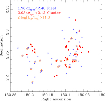
Figure 1. Spatial distribution of Hα-emitting cluster galaxies (filled circles; 37) and field galaxies (crosses; 53) at  in the COSMOS legacy field. Galaxies with total IR luminosities
  > 2 × 10¹¹
  as measured using Spitzer/24 μm (
 detection) are shown as open stars (21). AGNs are excluded using the AGN catalog by Cowley et al. (2016). The fraction of IR-luminous galaxies is the same in the field and the cluster (
 %–25%).
Download figure:
Standard image High-resolution imageWe note that our study focuses on cluster and field galaxies at  identified by their Hα emission, thus we cannot confidently measure the relative fraction of star-forming galaxies to all galaxies across environment with the current data set.
2.3. Measuring Galaxy Sizes and Morphologies
We use GALFIT (Peng et al. 2010) to measure Sérsic indices, effective radii, axis ratios, and position angles for the spectroscopically confirmed galaxies in COSMOS using Hubble Space Telescope imaging taken with WFC3/F160W. Most of these galaxies are in the morphological catalog of van der Wel et al. (2012), which spans a wide redshift range. However, we choose to measure the galaxy sizes and morphologies independently to optimize the fits for our galaxies at  .
.
Of the 90 galaxies in our Hα-emitting sample, we measure effective radii along the major axis and Sérsic indices for 83 (35 cluster, 48 field); see Figures 2 and 3 for galaxy images and Table 1 for galaxy properties. Seven of the galaxies could not be fit because of contamination due to diffraction spikes from nearby stars or incomplete F160W imaging (see Skelton et al. 2014). We include a quality flag on the GALFIT results and identify 12 galaxies with fits that have large residuals due to, e.g., being mergers (see Alcorn et al. 2016). We confirm that excluding these 12 galaxies does not change our general results and so we use the effective radii measured for all 83 galaxies in our analysis.

Figure 2. HST images ( ) generated by summing F125W, F140W, and F160W for Hα-emitting cluster galaxies (
 ); Sérsic indices and effective radii are measured using GALFIT for 35 of 37 members. Galaxies are labeled with their ZFIRE IDs, and IR-luminous galaxies (
 > 2 × 10¹¹
  ) are noted as LIRGs.
Download figure:
Standard image High-resolution image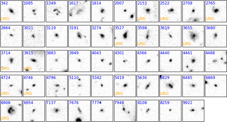
Figure 3. HST images ( ) generated by summing F125W, F140W, and F160W for Hα-emitting field galaxies at
  (
( ); Sérsic indices and effective radii are measured using GALFIT for 49 of 53 field galaxies. Galaxies are labeled with their ZFIRE IDs, and IR-luminous galaxies (
 > 2 × 10¹¹
  ) are noted as LIRGs.
Download figure:
Standard image High-resolution imageTable 1. Galaxy Properties
| ZFIRE a | ZFOURGE a | α(2000) | δ(2000) |

|
fHαb | err(fHα)b |
 ( ( / / )c )c
|

|

|
 d
d
|
SFR( )e )e
|
Sérsic n |
 ( ( ) ) |
Pflagf |
|---|---|---|---|---|---|---|---|---|---|---|---|---|---|---|
| 237 | 912 | 150.19057 | 2.18848 | 2.1572 | 1.46 | 0.17 | ⋯ | 9.65 | 0.6 | 8.1 | 6.0 | ⋯ | ⋯ | −99 |
| 342 | 1108 | 150.19051 | 2.19065 | 2.1549 | 3.98 | 0.09 | 11.93 | 10.45 | 1.1 | 8.9 | 31.3 | 0.8 | 0.4 | 0 |
| 1085 | 2114 | 150.18338 | 2.20192 | 2.1882 | 2.53 | 0.07 | ⋯ | 9.60 | 0.1 | 8.4 | 5.6 | 1.3 | 0.2 | 0 |
| 1180 | 2168 | 150.12984 | 2.20287 | 2.0976 | 1.33 | 0.15 | ⋯ | 8.94 | 0.0 | 8.1 | 2.3 | 4.0 | 0.2 | 2 |
| 1349 | 2517 | 150.20306 | 2.20554 | 2.1888 | 1.04 | 0.06 | 11.23 | 9.82 | 0.3 | 8.3 | 3.0 | 4.0 | 0.1 | 1 |
| 1385 | 2510 | 150.12344 | 2.20565 | 2.0978 | 3.28 | 0.23 | ⋯ | 9.30 | 0.1 | 8.0 | 6.5 | 0.5 | 0.3 | 0 |
| 1617 | 2989 | 150.09697 | 2.20917 | 2.1732 | 1.32 | 0.14 | 11.22 | 10.14 | 0.5 | 8.7 | 4.8 | 0.9 | 0.7 | 2 |
| 1814 | 3175 | 150.16809 | 2.21129 | 2.1704 | 4.55 | 0.10 | ⋯ | 9.95 | 0.4 | 8.5 | 14.6 | 1.0 | 0.3 | 0 |
| 2007 | 3375 | 150.16566 | 2.21366 | 2.0086 | 1.17 | 0.14 | 11.17 | 9.42 | 0.4 | 8.5 | 3.1 | 0.9 | 0.1 | 0 |
| 2153 | 3669 | 150.16533 | 2.21584 | 2.0123 | 4.86 | 0.18 | 11.48 | 10.07 | 0.7 | 8.8 | 19.2 | 4.0 | 0.9 | 2 |
| 2522 | 4084 | 150.19379 | 2.22011 | 2.1511 | 1.10 | 0.11 | 11.48 | 9.64 | 0.3 | 8.1 | 3.0 | 0.5 | 0.4 | 0 |
| 2709 | 4401 | 150.08572 | 2.22317 | 2.1970 | 2.45 | 0.12 | ⋯ | 9.68 | 0.3 | 8.3 | 7.1 | 2.6 | 0.2 | 0 |
| 2715 | 4484 | 150.08955 | 2.22356 | 2.0829 | 2.80 | 0.10 | 11.45 | 9.98 | 0.8 | 8.1 | 13.7 | 0.9 | 0.5 | 2 |
| 2765 | 4577 | 150.11935 | 2.22412 | 2.2285 | 11.12 | 0.15 | 12.00 | 10.68 | 1.0 | 9.0 | 83.3 | 4.0 | 0.3 | 2 |
| 2790 | 4533 | 150.09761 | 2.22423 | 2.0981 | 1.61 | 0.23 | ⋯ | 9.88 | 0.4 | 8.5 | 4.7 | 1.6 | 0.3 | 1 |
| 2864 | 4541 | 150.05670 | 2.22499 | 2.2005 | 1.33 | 0.13 | 10.35 | 9.53 | 0.6 | 8.6 | 5.7 | 0.5 | 0.2 | 0 |
| 3021 | 4741 | 150.11507 | 2.22711 | 2.3037 | 0.47 | 0.06 | ⋯ | 9.24 | 0.2 | 8.6 | 1.3 | 0.3 | 0.2 | 0 |
| 3052 | 4860 | 150.09961 | 2.22810 | 2.0978 | 1.86 | 0.16 | 11.45 | 9.68 | 0.3 | 8.0 | 4.8 | 0.5 | 0.5 | 0 |
| 3119 | 4933 | 150.08765 | 2.22895 | 2.1278 | 1.30 | 0.15 | ⋯ | 9.75 | 0.2 | 8.6 | 3.0 | 0.9 | 0.2 | 0 |
| 3191 | 5029 | 150.13834 | 2.22999 | 2.1449 | 2.77 | 0.11 | 11.12 | 9.94 | 0.6 | 8.3 | 11.2 | 0.4 | 0.4 | 0 |
| 3274 | 5152 | 150.18436 | 2.23134 | 2.1918 | 5.48 | 0.08 | ⋯ | 9.85 | 0.3 | 8.3 | 15.7 | 0.7 | 0.3 | 0 |
| 3527 | 5593 | 150.18259 | 2.23587 | 2.1889 | 7.82 | 0.08 | 12.04 | 10.40 | 1.0 | 8.0 | 56.1 | 0.9 | 0.4 | 2 |
| 3532 | 5420 | 150.07999 | 2.23515 | 2.1014 | 4.37 | 0.06 | 11.14 | 9.83 | 0.2 | 9.2 | 9.9 | 0.9 | 0.2 | 0 |
| 3577 | 5576 | 150.07526 | 2.23610 | 2.0955 | 3.88 | 0.11 | 11.91 | 10.54 | 1.0 | 9.1 | 25.0 | 0.6 | 0.4 | 0 |
| 3598 | 5672 | 150.11209 | 2.23685 | 2.2281 | 2.15 | 0.11 | 11.90 | 10.54 | 1.3 | 9.2 | 23.8 | 1.0 | 0.5 | 2 |
| 3619 | 5500 | 150.19704 | 2.23613 | 2.2939 | 1.32 | 0.10 | 11.10 | 9.32 | 0.1 | 8.5 | 3.3 | 0.7 | 0.3 | 0 |
| 3633 | 5633 | 150.12492 | 2.23698 | 2.1003 | 8.51 | 0.11 | 12.05 | 10.72 | 0.8 | 9.4 | 42.4 | 0.8 | 0.6 | 0 |
| 3655 | 5858 | 150.16914 | 2.23838 | 2.1267 | 8.61 | 0.17 | 11.87 | 10.89 | 0.1 | 8.8 | 17.7 | 0.7 | 0.5 | 0 |
| 3680 | 5595 | 150.06345 | 2.23703 | 2.1760 | 1.57 | 0.10 | 10.07 | 9.41 | 0.4 | 8.0 | 5.0 | 0.6 | 0.3 | 0 |
| 3714 | 5759 | 150.07079 | 2.23816 | 2.1767 | 5.55 | 0.11 | 11.39 | 10.19 | 1.4 | 8.0 | 66.3 | 0.9 | 0.3 | 1 |
| 3765 | 5711 | 150.10236 | 2.23818 | 2.0976 | 2.03 | 0.19 | ⋯ | 9.32 | 0.0 | 8.6 | 3.5 | 1.0 | 0.2 | 0 |
| 3815 | 5891 | 150.07903 | 2.23947 | 2.1774 | 5.03 | 0.14 | 11.63 | 10.02 | 0.3 | 8.5 | 14.2 | 1.8 | 0.3 | 0 |
| 3842 | 5941 | 150.09471 | 2.23990 | 2.1027 | 1.75 | 0.10 | 11.43 | 10.31 | 0.8 | 8.4 | 8.8 | 0.9 | 0.4 | 0 |
| 3883 | 5849 | 150.07362 | 2.23982 | 2.3005 | 1.34 | 0.08 | ⋯ | 9.22 | 0.0 | 8.4 | 2.9 | 0.9 | 0.2 | 0 |
| 3949 | 5964 | 150.12270 | 2.24089 | 2.1726 | 1.94 | 0.09 | 10.99 | 10.10 | 0.6 | 9.1 | 8.1 | 1.4 | 0.2 | 0 |
| 4035 | 6128 | 150.09526 | 2.24233 | 2.0981 | 2.83 | 0.14 | 11.02 | 9.56 | 0.3 | 8.0 | 7.3 | 1.0 | 0.3 | 0 |
| 4043 | 6065 | 150.13737 | 2.24214 | 2.2231 | 3.35 | 0.05 | ⋯ | 9.16 | 0.0 | 8.0 | 6.7 | 1.0 | 0.1 | 0 |
| 4091 | 6170 | 150.09436 | 2.24296 | 2.0979 | 2.05 | 0.10 | ⋯ | 9.29 | 0.0 | 8.4 | 3.6 | 0.3 | 0.3 | 0 |
| 4172 | 6255 | 150.09941 | 2.24415 | 2.0951 | 1.37 | 0.22 | 10.82 | 9.35 | 0.0 | 8.7 | 2.4 | 1.0 | 0.6 | 2 |
| 4260 | 6386 | 150.20407 | 2.24553 | 2.1856 | 2.16 | 0.14 | 8.76 | 9.45 | 0.0 | 9.0 | 4.2 | ⋯ | ⋯ | −99 |
| 4301 | 6405 | 150.07098 | 2.24599 | 1.9703 | 2.66 | 0.09 | ⋯ | 8.94 | 0.1 | 8.1 | 4.5 | 1.8 | 0.1 | 2 |
| 4366 | 6556 | 150.17508 | 2.24720 | 2.1248 | 2.28 | 0.17 | 11.09 | 9.58 | 0.1 | 8.5 | 4.7 | 1.0 | 0.2 | 0 |
| 4389 | 6686 | 150.21753 | 2.24787 | 2.1745 | 2.05 | 0.10 | 11.50 | 9.88 | 0.6 | 8.8 | 8.5 | ⋯ | ⋯ | −99 |
| 4440 | 6702 | 150.08844 | 2.24847 | 2.3010 | 9.44 | 0.10 | 11.22 | 9.45 | 0.0 | 8.3 | 20.6 | 1.4 | 0.1 | 0 |
| 4461 | 6938 | 150.07658 | 2.24967 | 2.3011 | 1.64 | 0.12 | 11.05 | 10.99 | 0.8 | 9.4 | 10.2 | 4.0 | 0.3 | 0 |
| 4488 | 6811 | 150.07721 | 2.24927 | 2.3073 | 1.84 | 0.12 | 11.21 | 10.41 | 0.5 | 9.4 | 7.8 | 0.6 | 0.4 | 0 |
| 4595 | 6820 | 150.06758 | 2.25030 | 2.0959 | 1.16 | 0.09 | 11.06 | 9.40 | 0.0 | 9.3 | 2.0 | 1.3 | 0.2 | 0 |
| 4645 | 6997 | 150.07433 | 2.25162 | 2.1018 | 1.62 | 0.08 | 11.20 | 9.61 | 0.5 | 8.3 | 5.5 | 0.4 | 0.3 | 0 |
| 4647 | 6961 | 150.20522 | 2.25134 | 2.0922 | 2.76 | 0.09 | 10.07 | 9.31 | 0.1 | 8.0 | 5.4 | ⋯ | ⋯ | −99 |
| 4655 | 6978 | 150.07341 | 2.25164 | 2.1019 | 0.68 | 0.08 | 11.20 | 9.45 | 0.0 | 8.8 | 1.2 | 0.6 | 0.1 | 0 |
| 4724 | 7071 | 150.07166 | 2.25250 | 2.3041 | 1.24 | 0.07 | 11.32 | 9.66 | 0.1 | 8.5 | 3.1 | 8.0 | 0.7 | 0 |
| 4746 | 7111 | 150.08624 | 2.25295 | 2.1771 | 1.90 | 0.08 | 10.48 | 9.60 | 0.4 | 8.3 | 6.1 | 0.9 | 0.1 | 0 |
| 4796 | 7281 | 150.14738 | 2.25441 | 2.1663 | 1.59 | 0.09 | ⋯ | 9.62 | 0.6 | 8.5 | 6.6 | 0.8 | 0.3 | 0 |
| 4930 | 7366 | 150.05595 | 2.25571 | 2.0974 | 3.63 | 0.06 | ⋯ | 9.58 | 0.1 | 8.5 | 7.2 | 1.0 | 0.4 | 2 |
| 4938 | 7423 | 150.18358 | 2.25618 | 2.0913 | 5.08 | 0.16 | 12.05 | 10.51 | 1.0 | 9.2 | 32.6 | 1.0 | 0.5 | 0 |
| 4961 | 7522 | 150.03694 | 2.25691 | 2.0956 | 2.66 | 0.12 | ⋯ | 9.79 | 0.3 | 8.9 | 6.9 | ⋯ | ⋯ | −99 |
| 5110 | 7577 | 150.07088 | 2.25849 | 2.3028 | 0.95 | 0.09 | 11.11 | 9.54 | 0.2 | 8.7 | 2.7 | 0.9 | 0.2 | 0 |
| 5165 | 7651 | 150.18961 | 2.25921 | 2.0949 | 1.75 | 0.11 | ⋯ | 9.64 | 0.7 | 8.7 | 7.6 | 0.9 | 0.3 | 0 |
| 5269 | 8019 | 150.06621 | 2.26215 | 2.1090 | 2.39 | 0.13 | 11.23 | 10.17 | 0.9 | 8.5 | 13.7 | 0.5 | 0.5 | 0 |
| 5298 | 7793 | 150.09132 | 2.26111 | 2.0861 | 2.09 | 0.06 | ⋯ | 9.01 | 0.0 | 8.6 | 3.6 | 1.6 | 0.1 | 0 |
| 5342 | 7868 | 150.07851 | 2.26189 | 2.1629 | 1.16 | 0.05 | 10.98 | 9.21 | 0.1 | 8.3 | 2.5 | 1.0 | 0.1 | 0 |
| 5381 | 8017 | 150.18343 | 2.26288 | 2.0889 | 4.31 | 0.25 | ⋯ | 9.43 | 0.2 | 8.1 | 9.7 | 1.9 | 0.2 | 0 |
| 5408 | 8020 | 150.06621 | 2.26312 | 2.0979 | 3.69 | 0.15 | 11.07 | 9.92 | 0.9 | 8.5 | 20.9 | 1.0 | 0.2 | 0 |
| 5419 | 8109 | 150.20366 | 2.26366 | 2.2128 | 3.27 | 0.16 | 11.47 | 10.00 | 0.7 | 8.3 | 16.3 | 2.1 | 0.2 | 0 |
| 5582 | 8239 | 150.22964 | 2.26539 | 2.1829 | 2.69 | 0.10 | 11.13 | 9.72 | 0.0 | 8.9 | 5.2 | ⋯ | ⋯ | −99 |
| 5609 | 8307 | 150.09839 | 2.26592 | 2.0895 | 8.96 | 0.25 | ⋯ | 9.52 | 0.1 | 8.2 | 17.6 | 1.7 | 0.1 | 0 |
| 5630 | 8407 | 150.20097 | 2.26653 | 2.2429 | 4.02 | 0.10 | 11.13 | 9.98 | 0.8 | 8.0 | 23.6 | 1.4 | 0.4 | 0 |
| 5643 | 8445 | 150.05336 | 2.26684 | 2.0960 | 0.59 | 0.08 | 10.67 | 9.57 | 0.3 | 8.5 | 1.5 | 1.1 | 0.4 | 0 |
| 5696 | 8452 | 150.05836 | 2.26722 | 2.0929 | 3.11 | 0.14 | ⋯ | 9.64 | 0.1 | 8.5 | 6.1 | 0.5 | 0.2 | 0 |
| 5745 | 8486 | 150.09871 | 2.26781 | 2.0920 | 4.96 | 0.16 | ⋯ | 9.10 | 0.0 | 8.1 | 8.6 | 2.7 | 0.1 | 0 |
| 5751 | 8618 | 150.09741 | 2.26844 | 2.0920 | 8.76 | 0.14 | 11.19 | 9.79 | 0.0 | 8.2 | 15.2 | 0.8 | 0.3 | 0 |
| 5808 | 8557 | 150.19075 | 2.26844 | 2.0915 | 0.99 | 0.11 | 11.05 | 9.16 | 0.0 | 8.6 | 1.7 | 0.3 | 0.4 | 0 |
| 5829 | 8730 | 150.06894 | 2.26927 | 2.1626 | 4.54 | 0.08 | 11.59 | 10.35 | 0.7 | 8.9 | 21.3 | 0.9 | 0.4 | 0 |
| 5870 | 8732 | 150.06094 | 2.26964 | 2.1042 | 2.03 | 0.09 | 10.93 | 9.98 | 0.6 | 8.6 | 7.8 | 0.7 | 0.4 | 0 |
| 5914 | 8764 | 150.09709 | 2.27018 | 2.0953 | 3.41 | 0.08 | ⋯ | 9.69 | 0.1 | 8.8 | 6.8 | 1.0 | 0.3 | 0 |
| 6114 | 9135 | 150.19441 | 2.27333 | 2.0984 | 1.05 | 0.14 | 12.22 | 10.74 | 1.6 | 8.5 | 14.9 | 1.0 | 0.5 | 2 |
| 6485 | 9502 | 150.06190 | 2.27839 | 2.1631 | 2.80 | 0.09 | 11.28 | 10.43 | 0.9 | 9.4 | 17.1 | 1.1 | 0.3 | 0 |
| 6523 | 9538 | 150.09041 | 2.27879 | 2.0877 | 2.45 | 0.14 | ⋯ | 9.44 | 0.0 | 8.7 | 4.2 | 0.8 | 0.1 | 0 |
| 6869 | 9993 | 150.07315 | 2.28436 | 2.1265 | 4.04 | 0.07 | 11.01 | 9.54 | 0.0 | 9.0 | 7.3 | 2.2 | 0.1 | 0 |
| 6908 | 10239 | 150.08344 | 2.28577 | 2.0637 | 5.71 | 0.05 | 12.15 | 10.67 | 1.4 | 8.5 | 59.9 | 0.5 | 0.5 | 0 |
| 6954 | 10125 | 150.10315 | 2.28551 | 2.1286 | 3.25 | 0.05 | ⋯ | 9.27 | 0.1 | 8.1 | 6.7 | 0.6 | 0.2 | 0 |
| 7137 | 10418 | 150.05479 | 2.28925 | 2.1620 | 2.26 | 0.07 | 11.08 | 9.92 | 0.6 | 8.3 | 9.3 | 1.1 | 0.4 | 0 |
| 7676 | 11212 | 150.06837 | 2.29838 | 2.1604 | 1.83 | 0.09 | 10.35 | 9.58 | 0.2 | 8.3 | 4.4 | 0.7 | 0.5 | 0 |
| 7774 | 11356 | 150.06976 | 2.29943 | 2.1990 | 2.22 | 0.15 | 11.13 | 10.34 | 0.7 | 9.4 | 10.9 | 1.2 | 0.2 | 0 |
| 7930 | 11658 | 150.06255 | 2.30233 | 2.1015 | 3.15 | 0.07 | 10.69 | 9.89 | 0.3 | 8.8 | 8.2 | 2.5 | 0.5 | 2 |
| 7948 | 11833 | 150.10864 | 2.30333 | 2.0642 | 3.82 | 0.18 | 11.25 | 10.19 | 0.8 | 8.1 | 18.3 | ⋯ | ⋯ | −99 |
| 8108 | 11800 | 150.06227 | 2.30440 | 2.1627 | 2.49 | 0.07 | 10.94 | 9.69 | 0.2 | 9.0 | 6.1 | 1.0 | 0.3 | 0 |
| 8259 | 11953 | 150.07748 | 2.30623 | 2.0051 | 1.15 | 0.10 | 10.63 | 9.28 | 0.2 | 8.8 | 2.3 | 0.7 | 0.1 | 0 |
| 9571 | 13919 | 150.07310 | 2.32644 | 2.0900 | 2.35 | 0.14 | ⋯ | 9.67 | 0.5 | 7.9 | 7.8 | 4.0 | 0.5 | 0 |
| 9922 | 14346 | 150.08963 | 2.33156 | 2.0416 | 6.69 | 0.06 | 10.97 | 9.73 | 0.4 | 8.7 | 18.4 | 1.7 | 0.2 | 0 |
Notes.
aWe list galaxy identification numbers from ZFIRE (Nanayakkara et al. 2016) and ZFOURGE (Straatman 2016). We include only galaxies with a spectroscopic redshift quality flag of (Nanayakkara et al. 2016) and
  . Cluster members have
  (Yuan et al. 2014).
bObserved Hα fluxes and errors are in units of
(Yuan et al. 2014).
bObserved Hα fluxes and errors are in units of  erg s−1 cm−2.
cIn our analysis of IR-luminous versus low-IR systems, we select IR-luminous galaxies using
erg s−1 cm−2.
cIn our analysis of IR-luminous versus low-IR systems, we select IR-luminous galaxies using  (
( /
/ )
)  .
dStellar age in units of Gyr and based on SED fitting with FAST (Kriek et al. 2009).
e
.
dStellar age in units of Gyr and based on SED fitting with FAST (Kriek et al. 2009).
e
 star formation rates in units of
  yr−1 and based on dust-corrected Hα fluxes (Equation (2); see Section 2.4).
fPflag denotes quality of profile fit used to measure the Sérsic index n and the effective radius
yr−1 and based on dust-corrected Hα fluxes (Equation (2); see Section 2.4).
fPflag denotes quality of profile fit used to measure the Sérsic index n and the effective radius  . Pflag values are −99 (not fit), 0 (good fit), 1 (fair fit), and 2 (questionable fit).
Only a portion of this table is shown here to demonstrate its form and content. A machine-readable version of the full table is available.
Following van der Wel et al. (2014), we use the effective radius to characterize size because  is more appropriate than a circularlized radius for galaxies spanning the range in axis ratios. We confirm that using
  instead of
  does not change the following results except for shifting the size distribution of the entire galaxy sample to smaller sizes. The trends in the scaling relations that depend on galaxy size, e.g., comparing cluster to field and galaxies relative to the SFMS, are robust.
2.4. Dust-corrected Hα Star Formation Rates
To use Hα line emission as a measure of SFR, we need to correct for dust attenuation. Although determining the internal extinction using the Balmer decrement is preferred, we have Hβ for only a small subset. Thus we must rely on the stellar attenuation  measured by FAST, which assumes
  = 4.05 (starburst attenuation curve; Calzetti et al. 2000).15
For more extensive results on stellar versus Balmer-derived attenuation and SFRs, we refer the reader to Price et al. (2014) and Reddy et al. (2015).
= 4.05 (starburst attenuation curve; Calzetti et al. 2000).15
For more extensive results on stellar versus Balmer-derived attenuation and SFRs, we refer the reader to Price et al. (2014) and Reddy et al. (2015).
Following Tran et al. (2015) (see also Steidel et al. 2014), the Hα line fluxes are corrected using the nebular attenuation curve from Cardelli et al. (1989) with  = 3.1:

We use the observed stellar to nebular attenuation ratio of 

 (Calzetti et al. 2000) and the color excess
  , which is the stellar attenuation
  measured by FAST divided by
  = 4.05. Combining these factors, we have

which we use to correct all of the Hα fluxes for attenuation. Recent work by Reddy et al. (2015) suggests that the ratio of  to
to  may depend on stellar mass at
  , but there is significant scatter in the fitted relation. We stress that such a correction would not change our results because we use the same method to measure Hα SFRs for all the galaxies in our study and compare internally.
We determine the corresponding SFRs using the relation from Hao et al. (2011):

This relation assumes a Kroupa IMF (0.1–100  ; Kroupa 2001), but the relation for a Chabrier IMF is virtually identical (a difference of 0.05). Note that values of
  [SFR(
[SFR( )] determined with the relation of Hao et al. (2011) are 0.17 dex lower than when using that of Kennicutt (1998).
2.5.
 SFR Surface Densities

With the  SFRs and galaxy sizes as measured by their effective radii (
 ), we can then determine the SFR surface density:

Note that most of the cluster and field galaxies have effective radii of 
 (Figure 4), which is comparable to the slit width of
  .
.

Figure 4. We measure the effective radii ( ) using Hubble Space Telescope imaging taken with WFC3/F160W. Left: the galaxy size–stellar mass relation for our combined sample is consistent with the fit to star-forming galaxies at
  measured using photometric redshifts by CANDELS and clearly offset from the relation at z = 0.25 (pink dash–dot curves; van der Wel et al. 2014). We find no significant difference between the size–mass relation for Hα-emitting cluster galaxies (red dashed) and field galaxies (blue dotted) at
  . Right: the
  –
– relations for galaxies on (open crosses) and below (filled triangles) the Hα star-forming main sequence (SFMS; see Figure 6) are consistent with CANDELS, but the galaxies with elevated SFRs (filled squares) have smaller radii at a given stellar mass. For reference, the black line is the (
 clipped) least-squares fit to our combined sample.
Download figure:
Standard image High-resolution imageIt is possible that by using  measured with WFC/F160W imaging we are overestimating Σ(
 ). Förster Schreiber et al. (2011) find that the Hα sizes of six
  galaxies are comparable to their rest-frame continuum sizes as measured with integral field unit (IFU) and HST observations. However, Nelson et al. (2016) show that, at
  , continuum-based sizes tend to be smaller than Hα-based sizes for star-forming galaxies with
 . While correcting for a possible dependence of Hα size on galaxy mass would shift Σ(
 ) to lower values, it would not change our overall conclusions based on comparing the different galaxy populations.
Note that with our current single-slit observations, we cannot address a possible environmental dependence of Hα disks. Galaxies in the Virgo cluster are known to have truncated Hα disks compared to the field (Kenney & Koopmann 1999; Koopmann & Kenney 2004), thus not accounting for disk truncation in the cluster galaxies may lead to overestimating their total  SFRs and consequently Σ(
 ). Future deep IFU observations with the next generation of large telescopes should be able to test for Hα-disk truncation in these
  galaxies.
2.6. IR Luminosities from Spitzer/MIPS
Summarizing from Tomczak et al. (2016), IR luminosities are determined from Spitzer/MIPS observations at 24 μm (GOODS-S: PI M. Dickinson, COSMOS: PI N. Scoville, UDS: PI J. Dunlop), which have  uncertainties of 10.3 μJy in COSMOS. We measure the 24 μm fluxes within
  apertures and use the custom code MOPHONGO (written by I. Labbé; see Labbé et al. 2006; Wuyts et al. 2007) to deblend fluxes from multiple sources. The templates of Wuyts et al. (2008) are fit to the SEDs using the Hα redshifts to determine integrated 8−1000 μm fluxes; we refer the reader to Tomczak et al. (2016) for a full description of the IR measurements.
For galaxies at  , the
, the 
 detection limit is 2 × 10¹¹
  , i.e., all our
  galaxies are LIRGs.16
Figure 1 shows the spatial distribution of IR-luminous cluster and field galaxies. In our analysis, we use IR-based luminosities and
galaxies are LIRGs.16
Figure 1 shows the spatial distribution of IR-luminous cluster and field galaxies. In our analysis, we use IR-based luminosities and  SFRs. We note that
  detection thresholds at
  correspond to SFRs that are much higher than UV-based SFRs. Thus comparing, e.g., an
  SFR to a combined (IR+UV) SFR instead of an
  -only SFR does not change our results.
3. RESULTS
3.1. A Population of IR-luminous Galaxies
A remarkable 19% (7/37) of Hα-emitting cluster galaxies at  have
have  > 2 × 10¹¹
  . Within errors, this fraction of IR-luminous cluster galaxies is comparable to the field (26%, 14/53; Figure 1). Saintonge et al. (2008) showed using 24 μm observations of ∼1500 spectroscopically confirmed cluster galaxies that the fraction of IR members increases with redshift, but this was limited to galaxy clusters at
  . More recent studies using the Herschel Space Observatory have detected IR sources in galaxy clusters at
  (Popesso et al. 2012; Santos et al. 2014), but far-IR observations can only detect a handful of the most IR-luminous systems with SFRs
 yr−1. Our survey is the first to spectroscopically confirm the high fraction of LIRGs in galaxy clusters at
  (see also Hung et al. 2016).
3.2. Comparing Star Formation Rates
3.2.1. Cluster versus Field
We find no evidence of different correlations between Hα and  when considering the cluster and field samples separately (Figure 5; Table 1). For the 14 field and seven cluster galaxies with
  > 2 × 10¹¹
  , a Kolmogorov–Smirnov (K-S) test measures a p-value of 0.13, i.e., the statistical likelihood of the cluster and field populations being drawn from different parent populations is low. The average
  (
( ) per galaxy is comparable: 11.7 ± 0.3 in the field versus 11.8 ± 0.3 in the cluster. This is true also when selecting instead by SFR(
 ) > 2
) > 2  yr−1: the field (52) and cluster (34) populations have the same median
  [SFR(
[SFR( )] of 0.9 ± 0.3. Note that K-S tests confirm that the Hα-emitting galaxies in the cluster and field are drawn from the same parent population in terms of their stellar mass and specific star formation rate (SSFR = SFR/
 ).
).
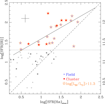
Figure 5. A Spearman rank test confirms that for the 21 galaxies with SFR( ) > 2
) > 2  yr−1 and
  > 2 × 10¹¹
  (horizontal dotted line), their SFRs based on these two tracers are correlated (
 confidence). The solid line shows the best least-squares fit (
 clipped) and the dashed diagonal line is parity; the cross in the upper left shows a representative log error of ±0.1 dex. Galaxies with
  < 2 × 10¹¹
  are shown in gray and have
  errors larger than the representative value. There is no evidence of environmental dependence: K-S tests confirm that the
  and
and  star formation rates have the same parent populations for cluster and field galaxies. The same is true if we compare the combined (IR+UV) star formation rate to
  values. However, SFRs based on
  are systematically lower than those from
  .
.
Download figure:
Standard image High-resolution image3.2.2. Hα versus

For galaxies with both  > 2
> 2  yr−1 and
  > 2 × 10¹¹
  (21), a Spearman rank test confirms a positive correlation (
 ) between SFRs based on these two tracers (Figure 5, Table 1; see also Ibar et al. 2013; Shivaei et al. 2016). However, the dust-corrected
  SFRs are systematically lower than
  SFRs by ∼0.5 dex, i.e., by nearly a factor of 3. This is driven mostly by a combination of using the relation of Hao et al. (2011) for converting Hα luminosities to SFRs instead of, e.g., that of Kennicutt (1998), and by choice of dust law. We confirm that comparing
  to a combined (IR+UV) SFR does not change our results.
We measure a scatter of  dex in
  –
– SFRs, which is larger than
  dex measured recently by Shivaei et al. (2016) for 17 galaxies at
  . However, their analysis focuses on galaxies with SFRs
 yr−1 while we push to
  SFRs of ∼2
  yr−1. From Figure 5, the discrepancy between
  and
and  SFRs decreases at higher values.
3.3. Hα SFMS at

Using deep multi-wavelength imaging, the relation between SFR and stellar mass is now measured to  for thousands of galaxies down to
  ∼ 9 (e.g., Whitaker et al. 2012; Tomczak et al. 2016, see Figure 6). However, the SFRs and stellar masses derived by fitting SEDs to multi-wavelength imaging can be degenerate. Measurements of Hα fluxes are a more accurate tracer of the instantaneous SFR than fitting SEDs to photometry (Kennicutt & Evans 2012), but are restricted to a smaller sample of galaxies due to the observational challenge of measuring Hα at
  .
.

Figure 6. Left: at  , galaxies in the COSMOS cluster (red filled circles) and field galaxies (blue line stars) follow identical relations between stellar mass and
  star formation rate;
  -clipped least-squares fits are shown by red dashed and blue dotted lines, respectively. The cross in the lower right shows a representative log error of ±0.1 dex. Both fits are consistent with the shape of the SFR–
 relation measured by ZFOURGE for star-forming field galaxies at
  using photometric redshifts (pink curve; Tomczak et al. 2016) as well as the mass-binned sample from MOSDEF for Hα-selected field galaxies at
  (open triangles; Sanders et al. 2015). Because we use Hao et al. (2011) to convert Hα luminosity to SFR, we are offset in
  [SFR(
[SFR( )] from both ZFOURGE and MOSDEF. The more massive galaxies (
 ) tend to be IR-luminous (
 > 2 × 10¹¹
  ; open orange stars), i.e., they are LIRGs. Right: we fit the Hα SFMS using our combined cluster and field sample (cyan line). In our analysis, we consider star-forming galaxies that lie above (+SFMS; purple filled squares), on (= SFMS; cyan open crosses), or below (–SFMS; yellow filled triangles) the Hα SFMS. Also shown is the predicted SFMS relation at
  from Rhapsody-G, a high-resolution AMR simulation of galaxy clusters (gray long dash–dot line; Martizzi et al. 2016).
Download figure:
Standard image High-resolution imageCombining SFRs based on  fluxes and stellar masses derived from SED fitting, we fit the SFR–
 relation using a (
 -clipped) least-squares fit for the field and cluster populations separately. Note that the field and cluster galaxies span the full range in both stellar mass and
  SFR (Figure 6). The cluster and field galaxies at
  have the same increasing SFR–
 relation:


where SFR is in  yr−1 and
  is in
is in  . The rms error on the fitted slopes is ∼0.2, and separate 1D K-S tests confirm that the stellar mass and SFR distributions of our cluster and field populations are similar. A possible concern is that our field sample could be contaminated by cluster members, but we confirm that applying a more stringent redshift cut of
  to select field galaxies does not change our results.
Our measurements are consistent with recent results, e.g., from ZFOURGE(SED fitting of UV–mid-IR; Tomczak et al. 2016) and MOSDEF (Hα; Sanders et al. 2015), and span similar ranges in stellar mass and SFR. However, our  SFRs are lower. This offset is mostly likely due to differences in the relation used to convert Hα luminosities to SFRs, e.g., Hao et al. (2011) versus Kennicutt (1998), and the choice of dust law. Accounting for both these effects increases
  [SFR(
[SFR( )] by ∼0.3 dex, which brings our SFMS into agreement with ZFOURGE and MOSDEF. These systematic differences in SFRs due to using different conversion relations and dust laws highlight the need to identify a more robust method of measuring SFRs at
  (e.g., Reddy et al. 2015; Shivaei et al. 2016).
In our analysis, we also compare star-forming galaxies that lie above, on, or below the SFMS as measured by Hα emission. Using the best fit to the combined cluster and field sample (Equation (7)), we calculate a galaxy's offset from the Hα SFMS given its stellar mass. Because the typical scatter in the Hα SFMS is ∼0.2 dex, we use ΔSFR( ) = 0.2 dex to separate galaxies into those above (20), on (45), or below (18) the SFMS. Galaxies in these three classes (+SFMS, = SFMS, –SFMS) span the full range in stellar mass (Figure 6, right).
The LIRGs also span the full range in stellar mass and  SFR for both field and cluster galaxies, and the most massive galaxies (
 ) tend to be LIRGs (Figure 6, left). The LIRGs at
  follow the same trend of increasing
  SFR with stellar mass (Figure 6; slope ∼0.80), a somewhat surprising result given the large scatter when comparing SFRs derived from
  to
to  (see Section 3.2). LIRGs lie above, on, or below the SFMS as defined by their
  SFRs (Figure 6, right).
3.4. Galaxy Size–Stellar Mass Relation
How galaxy size correlates with stellar mass depends on galaxy type, e.g., quiescent galaxies with Sérsic indices of  tend to be smaller at a given stellar mass than star-forming galaxies with
  (Shen et al. 2003). With a limited spectroscopic sample of galaxies, Law et al. (2012) showed that the galaxy size–mass relation evolves with redshift. Most recently, van der Wel et al. (2014) used high-resolution imaging from the Hubble Space Telescope and photometric redshifts for ∼31,000 galaxies to measure how the
  –
– relation of star-forming galaxies has evolved since
  .
.
We measure Sérsic indices and effective radii for 83 of the 90 galaxies in our sample (see Section 2.3 and Table 1). We find that our Hα-emitting  galaxies follow the same trend of increasing galaxy size with stellar mass measured by van der Wel et al. (2014) for galaxies at this epoch (Figure 4). Most of our fitted galaxies (71 of 83) have Sérsic indices of
  , and most (80 of 83) have effective radii of

 (Figure 7).
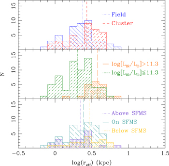
Figure 7. Top: Hα-selected cluster and field galaxies at  have the same size distribution as measured by the effective radius (
 ); medians are shown as vertical lines. Middle: however, in the combined sample, the IR-luminous galaxies (
 > 2 × 10¹¹
  ) tend to be ∼0.25 dex larger (∼70% larger in linear space) than the low-IR galaxies. A K-S test confirms at
  significance that the LIRGs and low-IR galaxies have different size distributions. The LIRGs also tend to be more massive (see Figure 6). Bottom: galaxies above, on, or below the Hα SFMS span a similar range in galaxy size, but +SFMS galaxies tend to have smaller
  at a given stellar mass than –SFMS galaxies (Figure 4).
Download figure:
Standard image High-resolution image3.4.1. Cluster versus Field
We find no difference in the galaxy size–stellar mass relation with environment for Hα-emitting galaxies. The cluster and field populations have the same size distributions with similar average effective radii of 
 and
and 
 , respectively (Figure 7). Least-squares fits to the
  –
– distribution for the cluster and field populations agree with the size–mass relation of van der Wel et al. (2014) within the errors.
The astute reader may notice possible conflict with our results in Allen et al. (2015), which reported that star-forming cluster galaxies are ∼12% larger than in the field. However, we do find evidence that at fixed stellar mass, our cluster galaxies are ∼0.1 dex larger, which is consistent with Allen et al. (2015). We refer to Section 3.4.4 below for details.
3.4.2. IR-luminous Galaxies
IR-luminous galaxies (LIRGs) have different physical size and stellar mass distributions to the low-IR population. A K-S test of the size distributions (Figure 7) confirms with  significance that the LIRGs are larger with a median
  ∼ 3.8 kpc compared to ∼2.0 kpc for the low-IR galaxies (typical errors for both are ∼0.3 kpc). LIRGs also are ∼5 times more massive with
  ∼ 10.4 compared to ∼9.6 for the low-IR galaxies (Figures 4 and 6). Even if we consider only galaxies with
 , LIRGs and low-IR galaxies have statistically different absolute
  distributions.
The size difference between our LIRGs and the low-IR galaxies at  seems to be in conflict with Swinbank et al. (2010) who, using Hubble Space Telescope/WFC3/F160W imaging of 25 submillimeter galaxies at
  , find that their submillimeter galaxies have the same sizes as field galaxies at
  (both have typical half-light radii of
  –2.8 kpc). We find that our LIRGs are typically ∼70% larger than the low-IR population (see also Kartaltepe et al. 2012). This discrepancy is likely due to our IR comparison being based on a mass-selected sample that identifies LIRGs to
  ∼ 9.5 (Figure 6) while Swinbank et al. (2010) is limited to galaxies with
 , i.e., galaxies that are large regardless of their
  emission because they are massive.
3.4.3. Above, on, and below the Hα SFMS
Galaxies above, on, or below the Hα SFMS (see Figure 6, right) also follow the same general trend of increasing galaxy size with stellar mass (Figure 4, right). K-S tests confirm that the size distributions for all three groups are likely drawn from the same parent population.
One concern in using Hα SFRs obtained with slit spectroscopy is that we are biased toward compact star-forming galaxies, e.g., significant slit losses in the spectroscopic flux measurements will cause smaller galaxies to appear to have higher Hα SFRs than larger galaxies. However, the slit width of  is comparable to the typical effective radius of most of the galaxies (
 Figure 4). Most importantly, we flux-calibrate our spectroscopic measurements using total galaxy fluxes anchored in deep ground- and space-based photometry and confirm that the uncertainty in the spectrophotometric calibration is 0.08 mag (see Section 2.7 in Nanayakkara et al. 2016).
3.4.4. Galaxy Size at Fixed Stellar Mass
To identify more subtle differences in galaxy size at fixed stellar mass, we first make a ( -clipped) least-squares fit to
  –
– using our combined cluster and field sample:
Our least-squares fit is virtually the same as the relation measured by van der Wel et al. (2014) for galaxies at z = 2.0 (Figure 4, right).
When controlling for stellar mass, we find that the  (
( ,
,  )] distributions for the cluster and field galaxies are likely drawn from different parent populations (Figure 8, top; p = 0.01); this is in contrast to no difference in their absolute
  distributions (Figure 7). At fixed
  , Hα-emitting cluster galaxies are ∼0.1 dex larger than their field counterparts. Our result is consistent with Allen et al. (2015), who find that star-forming cluster galaxies as identified by their UVJ colors are ∼12% larger than those in the field.

Figure 8. The same as Figure 7 but showing the difference in  at a fixed stellar mass. Here
  (
( ,
,  )] is determined using the (
 -clipped) least-squares fit to
  –
– of our combined cluster and field galaxies (Figure 4, black line in right panel). K-S tests now measure higher likelihoods, compared to their absolute
  distributions (Figure 7), that the cluster and field galaxies are drawn from different
  (
( ,
,  )] parent populations (p = 0.01); this is also true for galaxies above the SFMS vs. galaxies below it (p = 0.05). The
  (
( ,
,  )] distributions of the low-IR galaxies and LIRGs are more similar (p = 0.06).
Download figure:
Standard image High-resolution imageThere is also a higher likelihood that, at fixed stellar mass, galaxies above the SFMS are drawn from a different  (
( ,
,  )] parent population than those below (Figure 8, bottom; p = 0.05). The +SFMS galaxies are ∼0.1 dex smaller at a fixed
  than –SFMS galaxies (Figure 4). The compact nature of the +SFMS galaxies across the entire stellar mass range suggests that their star formation is more centralized than in the –SFMS galaxies (see also Section 4.2).
A K-S test of the  (
( ,
,  )] distributions for the low-IR galaxies versus LIRGs measures p = 0.06, which is not as statistically significant as when comparing their absolute
  distributions (
 ). Because LIRGs are more massive (Figure 6), they also tend to have larger radii. Thus controlling for stellar mass reduces differences in the LIRG and low-IR populations.
3.5. Galaxy Morphology and Stellar Ages
Having measured Sérsic indices for 83 galaxies in our Hα-emitting sample, we can compare the galaxy morphologies of the different populations. We find that all the galaxy populations (field versus cluster, LIRG versus low-IR, above/on/below SFMS) have comparable distributions in Sérsic index as measured by a K-S test. Most of the galaxies (71/83) are disk-dominated systems ( ).
).
The SED-based ages from ZFOURGE (Straatman 2016) confirm that the cluster and field galaxies have similar age distributions of ∼8.5 Gyr. This is also true for the LIRG and low-IR populations (both are ∼8.5 Gyr). However, comparison of the galaxies above (+SFMS), on (=SFMS), and below (−SFMS) the SFMS shows that their average stellar age increases, being ∼8.3, ∼8.6, and ∼8.7 Gyr respectively. The younger light-weighted stellar age of the +SFMS galaxies is consistent with a starburst nature.
3.6. Spatial Extent of Star Formation

Using the SFRs derived from  , the effective radii measured using WFC3/F160W imaging, and stellar masses from SED fitting, we first compare the
  SFR to galaxy size (
 , Figure 9; see Section 2.3 and Table 1). Our assumption that the Hα radii are comparable to the rest-frame optical radii is supported by results from SINS by Förster Schreiber et al. (2011), who combined IFU and HST observations of six Hα-emitting galaxies at
  and found no significant differences in their sizes or structural parameters at these wavelengths.
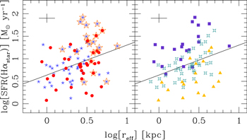
Figure 9. Left: there are no differences in the cluster (filled red circles) and field (filled blue stars) galaxies when comparing their  SFR to their WFC3/F160W galaxy size. The solid line in both panels is the least-squares fit (
 outliers removed) to the combined sample. LIRGs (open orange stars) tend to be larger than low-IR galaxies in both environments. Right: galaxies above (filled squares), on (open crosses), or below (filled triangles) the Hα SFMS (see Figure 6, right) populate different regions: +SFMS galaxies have higher
  SFRs at a given size than –SFMS galaxies.
Download figure:
Standard image High-resolution imageThe cluster and field galaxies have similar distributions, and least-squares fits ( outliers removed) confirm that both populations have the same slopes within the errors. As seen in Figure 7, the LIRGs tend to have larger
  than the low-IR galaxies because the LIRGs are more massive. In contrast, galaxies above the SFMS have higher
  SFRs at a given size than those below the SFMS (Figure 9).
We find similar results when comparing the SFR surface density (Σ( ); see Equation (4)) to galaxy size (
 , Figure 10) and stellar mass (
 , Figure 11). The cluster and field galaxies have similar distributions, and least-squares fits (
 -clipped) to Σ(
 )–
)– and Σ(
 )–
)– confirm that both populations have the same slopes within the errors. Note that our sample spans a range in galaxy size (0.5 <
  (kpc) < 8), SFR surface density (0.01 < Σ(
 ) < 5) where the units are
  yr−1 kpc−2, and stellar mass (9 <
  < 11).

Figure 10. Left: the SFR surface density Σ( ) is measured with
  SFR and WFC3/F160W galaxy size, and the solid line is the least-squares fit (
 outliers removed) to the combined sample. Cluster galaxies (filled circles) and field galaxies (line stars) have the same distribution in Σ(
 )–
)– . In contrast, the LIRGs (open stars) tend to be larger and have higher Σ(
 ) than low-IR galaxies, i.e., massive star-forming galaxies tend to have larger
  and also be LIRGs. Right: galaxies above (filled squares), on (open crosses), or below (filled triangles) the Hα SFMS (see Figure 6, right) populate different regions: +SFMS galaxies are forming stars more intensely than –SFMS galaxies across the range in galaxy size.
Download figure:
Standard image High-resolution image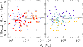
Figure 11. Left: the SFR surface density Σ( ) compared to stellar mass
  where the solid line is the least-squares fit (
 outliers removed) to the combined sample. Cluster galaxies (filled circles) and field galaxies (line stars) have the same distribution in Σ(
 )–
)– . LIRGs (open stars) are more massive than low-IR galaxies, but both populations span the range in Σ(
 ). Right: galaxies above (filled squares), on (open crosses), or below (filled triangles) the Hα SFMS (see Figure 6, right) populate different regions: +SFMS galaxies are forming stars more intensely than –SFMS galaxies across the range in stellar mass.
Download figure:
Standard image High-resolution imageIn contrast, the LIRGs and low-IR populations are different: at a given galaxy size, LIRGs tend to have higher SFR surface densities (Figure 10, left). As noted in Section 3.4.2, LIRGs also are typically ∼5 times more massive (Figure 11) and physically larger by ∼70%. However, LIRGs are not all starbursts, i.e., LIRGs are found above, on, and below the SFMS (Figure 6).
If we consider instead galaxies that lie above the SFMS, these +SFMS systems have higher SFR surface densities than –SFMS galaxies (Figure 10, right). At a given stellar mass, the +SFMS galaxies tend to have smaller radii (Figure 4) and higher Σ( ) (Figure 11) than galaxies on/below the SFMS. Our results suggest that the Hα star formation in +SFMS is more concentrated than in those on/below the SFMS.
3.7. Rhapsody Simulations: SFR–M*
We compare our relation between measured  SFR and stellar mass with predictions from the Rhapsody-G simulations of massive galaxy clusters (
 at z = 0; Hahn et al. 2015; Martizzi et al. 2016). These cosmological hydrodynamical zoom-in simulations (R4K resolution) use the Ramses adaptive mesh refined (AMR) code (Teyssier 2002) to reach a spatial resolution of 3.8
  kpc (physical), a mass resolution for dark matter particles of

 , and a baryonic mass resolution of

 . The simulations assume the standard ΛCDM cosmology (
 ,
,  ,
,  , h = 0.7) and include gas cooling, star formation, metal enrichment, and feedback from supernovae and AGNs.
The Rhapsody-G cluster simulations are well matched to our COSMOS cluster at  . As detailed in Yuan et al. (2014, see their Section 4), its measured velocity dispersion of
  km s−1 corresponds to a virial mass of

 . Merger trees from the GiggleZ gigaparsec simulation (Poole et al. 2015) show that such systems grow into a Virgo-mass cluster with

 by
by  .
.
We consider only simulated cluster galaxies at z = 2 with SFRs 
 yr−1; these galaxies have stellar masses of
  = 9–12. Here we assume that selecting by SFR is equivalent to the instantaneous observed SFR as measured by
  . We cannot apply the same observed UVJ selection because rest-frame colors are not available for the simulated galaxies.
From three Rhapsody-G cluster realizations, the least-squares fit to the SFR– relation is
The Rhapsody-G slope to the SFR– relation is steeper than that of the observed galaxies at
  : 1.08 versus 0.61 (Figure 6, right panel: gray and cyan lines respectively). Although the slopes are consistent within the scatter of the simulations and observations (see Section 3.3), the SFRs predicted by Rhapsody-G are lower by a factor of ∼2 for most of the observed galaxies. This difference between predicted and observed SFRs at a given stellar mass (i.e., the specific SFR) is known to exist for field comparisons (e.g., Davé et al. 2016). Here we show that this discrepancy extends to the cluster environment as well, i.e., simulations overpredict how efficiently galaxies quench at a given stellar mass for both the cluster and field environments (see Somerville & Davé 2015, and references therein). In the case of Rhapsody-G, star formation histories at high redshift are slightly under-resolved due to the mass resolution. Future simulations with higher resolution combined with multi-epoch observations are needed to improve galaxy formation modeling at
  . We will explore more key scaling relations and compare them to simulations in future work.
4. DISCUSSION
Our analysis focuses on comparing at  (i) cluster to field galaxies (37 versus 53); (ii) galaxies with
  > 2 × 10¹¹
  (LIRGs) to the low-IR population (21 versus 69); and (iii) galaxies above, on, and below the Hα SFMS. Because ours is a stellar mass-selected sample of Hα-emitting galaxies (
 see Figure 6), we are not limited to the high-mass end of the galaxy population. We consider only Hα-selected galaxies at
  because the redshifts for the quiescent galaxies are based on photometry and/or grism spectroscopy (Tomczak et al. 2014; Momcheva et al. 2016), neither of which is as precise as our Keck/MOSFIRE redshifts determined with Hα. We confirm that selecting field galaxies using a more stringent cut of
  from the mean cluster redshift does not change our results.
4.1. Hα-emitting Galaxies: Little Evidence of Environmental Dependence at

Our original motivation was to quantify how galaxy properties vary with environment at  . However, we find little evidence for environmental dependence in Hα-emitting galaxies at
  . We consistently measure the same relations for cluster and field galaxies when comparing their
  SFR to stellar mass (Figure 6), galaxy size to stellar mass (Figures 4 and 7), and star formation concentration (Figures 9–11). The fraction of LIRGs and their median
  are also the same in the cluster and field (Section 3.1). In our study, the only measurable difference is that Hα-emitting cluster galaxies are ∼0.1 dex larger than the field at fixed stellar mass (Figure 8).
In terms of their physical properties, the Hα-emitting cluster galaxies at  are essentially the same population as the field. This is consistent with our results in Kacprzak et al. (2015), which show that these very same cluster and field galaxies also follow the same relation between gas-phase metallicity and stellar mass (MZR). In addition, we find no evidence for an environmental dependence when comparing their kinematic scaling relations (Alcorn et al. 2016; Straatman et al. 2017).
The handful of existing studies on galaxy overdensities at  similarly find little evidence for environmental effects. Using narrow-band imaging, Koyama et al. (2013) measure the same SFR–
 relation for Hα emitters in a z = 2.16 protocluster as in the field. Using high-resolution imaging from the Hubble Space Telescope, Peter et al. (2007) measure the same size (radius) distributions for field and protocluster galaxies at z = 2.3.
In contrast, Papovich et al. (2012) find that quiescent cluster galaxies at z = 1.62 are larger than their field counterparts, and Quadri et al. (2012) find a higher fraction of quiescent galaxies in the same cluster. Several studies also find evidence of enhanced star formation in cluster galaxies at  (Tran et al. 2010, 2015; Brodwin et al. 2013; Santos et al. 2014; Webb et al. 2015). The lack of convincing evidence for strong environmental effects at
  combined with the increasing differences between cluster and field galaxies at lower redshifts points to
  as the critical epoch for ending star formation in cluster galaxies and building the spheroid population in clusters.
4.2. Tracking Galaxy Growth with the Hα SFMS
Given that the physical properties of Hα-emitting galaxies show little environmental dependence (see above), we can use the combined cluster and field sample at  to compare galaxies above, on, and below the SFMS as well as to compare the IR-luminous (21; LIRG) to low-IR (69) populations (Figures 6 through 11). Because our spectroscopic target selection is based on ZFOURGE, we are mass-limited to
  ∼ 9 at
  (Tomczak et al. 2014; Nanayakkara et al. 2016).
That a galaxy is a LIRG does not necessarily mean that it is a starburst, because LIRGs are found above, on, and below the SFMS (Figure 6, left). Rather, IR luminosity tends to track stellar mass closely such that massive galaxies ( ) tend to be LIRGs. On average, LIRGs are ∼5 times more massive and ∼70% larger than low-IR galaxies (Figures 4, 7, and 9). When controlling for stellar mass, there is less difference in the size distributions of the LIRGs and low-IR galaxies (Figure 8). Note that the mass range of our Hα-emitting galaxies reaches
  ∼ 9, i.e., a factor of about 5–10 times lower than previous studies that compared LIRGs to the general galaxy population at
  (e.g., Swinbank et al. 2010).
In terms of tracking how galaxies grow, systems that lie above the Hα star-forming main sequence (+SFMS) have smaller radii at a given stellar mass than those that are below it (Figure 4, right; see Section 3.4.3). The +SFMS galaxies tend to have higher  SFRs at a given galaxy size (Figure 9) and higher
  SFR surface densities than those below (Σ(
 ); Figures 10 and 11), i.e., their star formation is more compact. The +SFMS galaxies also have younger SED-based stellar ages of ∼8.3 Gyr compared to ∼8.7 Gyr for –SFMS galaxies. Taken as a whole, our results indicate that +SFMS galaxies are starbursts with Hα star formation concentrated in their cores (see also Barro et al. 2015).
At  , field galaxies are preferentially growing their disks (Nelson et al. 2016). In combination with our observations indicating that starbursts at
  are growing their stellar cores, these results suggest a sequence where +SFMS galaxies are building up their stellar cores at
  and then their stellar disks at
  , i.e., inside-out growth, likely by continuing gas accretion at
  (e.g., Kacprzak et al. 2016). Such a scenario naturally produces older stellar populations in the bulges than in the disks. This can also explain the rise of spheroids in clusters if the cluster environment prevents the growth of stellar disks even as star formation in the galaxies' cores is quenched at
  (Brodwin et al. 2013; Tran et al. 2015). While our hypothesis is based on the +SFMS galaxies, we note that galaxies at
  in general must grow physically larger by
  (e.g., van der Wel et al. 2014).
4.3. Star Formation Rates at : Caveat Emptor

Our analysis is based on the relative comparison of cluster and field galaxies where properties for both are determined in the same manner. Thus our results do not depend on the absolute conversion of, e.g., Hα flux to SFR. However, we do find that the  SFRs are offset from
  SFRs (Figure 5). The large uncertainty and likely offset from relations measured at
  bring into question our ability to measure reliable SFRs at
  .
.
There are several ongoing efforts to better understand star formation and dust laws at  that should help with calibrating existing relations. Recent studies at
  find evidence of changing ionization conditions (Sanders et al. 2016) as well as different dust laws (Reddy et al. 2015; Forrest et al. 2016; Shivaei et al. 2016) that can be incorporated into models. However, until we identify a more robust method for measuring SFRs in the distant universe, direct comparisons between studies will require carefully accounting for different methods of measuring SFRs.
5. CONCLUSIONS
Our ZFIRE program combines Keck/MOSFIRE spectroscopy with the wealth of multi-wavelength observations available in the COSMOS legacy field to explore galaxy scaling relations as a function of environment at  . Our advantage is that we select galaxies at
  based on their stellar masses as measured by ZFOURGE, a deep imaging survey that uses medium-band NIR filters to obtain high-precision photometric redshifts (
 Straatman 2016). We focus on the spectroscopically confirmed galaxy cluster at z = 2.095 in the COSMOS legacy field (Spitler et al. 2012; Yuan et al. 2014) and compare to the field population at
  .
.
In comparing Hα-emitting cluster (37) and field (53) galaxies (
 AGNs removed), we find little evidence of environmental influence on any of the galaxy scaling relations. Both cluster and field populations are consistent with published relations between SFR and stellar mass (SFR–
 ; Figure 6) as well as between galaxy size and stellar mass (
 –
– ; Figure 4) at
  . The cluster and field populations also have the same distribution when we compare their
  SFR surface density (Σ(
 )) to galaxy size and stellar mass (Figures 10 and 11). The results in this analysis mirror our existing ZFIRE results that show that these same cluster and field galaxies have the same relations between gas-phase metallicity and stellar mass (Kacprzak et al. 2015) and between kinematic mass and stellar mass (Alcorn et al. 2016), and also the same ISM conditions (Kewley et al. 2016). The only subtle indication of possible environmental dependence is that at fixed stellar mass, the Hα-emitting cluster galaxies are ∼0.1 dex larger than those in the field (Figure 8).
Using Spitzer/24 μm observations, we identify 21 galaxies with  > 2 × 10¹¹
  , i.e., LIRGs. Note that our mass range of
  ∼ 9 is a factor of about 5–10 times lower than previous studies that compared LIRGs to the general galaxy population at
  (e.g., Swinbank et al. 2010). The LIRG fraction is comparable within errors between the cluster and the field (19% and 26% respectively), and we do not find any indication that LIRGs in the cluster are different from those in the field. IR luminosity tracks with stellar mass such that our most massive galaxies (
 ) are dominated by LIRGs. As a result, LIRGs tend to be ∼5 times more massive with radii that are ∼70% larger than low-IR galaxies (
 ∼ 3.8 kpc versus ∼2.0 kpc; Figure 7). The LIRGs are not all starbursts because they are found above, on, and below the Hα SFMS (Figure 6).
We show that separating galaxies into those above the Hα SFMS (+SFMS), those on it, and those below it (–SFMS) provides insight into how galaxies grow (Figure 6). Galaxies in the three groups span the full range in parameter space, but the +SFMS galaxies have smaller radii at a given stellar mass than the –SFMS galaxies (Figure 4). The +SFMS galaxies also tend to have higher SFR surface densities than galaxies with depressed SFRs (Figures 9–11), and younger SED-based stellar ages than galaxies below the SFMS (∼8.3 Gyr versus ∼8.7 Gyr).
These lines of evidence indicate that +SFMS galaxies (starbursts) have concentrated Hα star formation and are actively growing their cores at  . We infer that while starbursts in the field go on to grow their stellar disks at
  (Nelson et al. 2016), cluster starbursts are likely to be quenching their star formation at
  (Brodwin et al. 2013; Tran et al. 2015) to then evolve into quiescent spheroids (Papovich et al. 2012; Quadri et al. 2012).
We compare the Hα SFR– relation to predictions from the Rhapsody-G simulations of massive galaxy clusters (
 at z = 0) based on the Ramses adaptive mesh refinement code. We find that the predicted slope for the SFR–
 relation is steeper than the observed values (1.08 versus 0.61), and that the predicted SFRs are about half those observed. Simulations in general continue to overpredict how efficiently galaxies quench at a given stellar mass in both the cluster and field environments. We will continue to explore how observed galaxy scaling relations compare to simulations in future work.
On a cautionary note, there is considerable scatter and likely offset in SFRs based on Hα and those based on IR luminosity (or UV+IR) at  (Figure 5). This is in contrast to the relatively small scatter at
  between Hα and 24 μm derived SFRs for activity at
 yr−1 (e.g., Hao et al. 2011). It is sobering to consider the large uncertainty in measuring robust SFRs, especially at higher redshifts when SFRs are increasing in general (Garn & Best 2010; Whitaker et al. 2014; Tomczak et al. 2016). Our ability to accurately measure star formation at
  is likely to be limited due to, e.g., our understanding of how ionization conditions evolve. However, we stress that the strength of this analysis lies in using the same observables to directly compare across different galaxy populations at
  .
.
In a companion ZFIRE paper, we estimate gas masses and gas depletion timescales for the same cluster and field galaxies at  . Ongoing analyses also include a comparison of the Tully–Fisher relation (Straatman et al. 2017) and constraints on the IMF (Nanayakkara et al. 2017). By measuring galaxy scaling relations for cluster and field galaxies at
  , ZFIRE provides a unique benchmark for quantifying galaxy evolution as a function of environment.
We are grateful to the MOSFIRE team with special thanks to M. Kassis, J. Lyke, G. Wirth, and L. Rizzi on the Keck support staff. K. Tran thanks M. Kriek, A. Shapley, S. Price, B. Forrest, and Jimmy for helpful discussions. We also thank the referee for a thoughtful and constructive report. This work was supported by a NASA Keck PI Data Award administered by the NASA Exoplanet Science Institute. Data presented herein were obtained at the W. M. Keck Observatory from telescope time allocated to NASA through the agency's scientific partnership with the California Institute of Technology and the University of California. The Observatory was made possible by the generous financial support of the W. M. Keck Foundation. K. Tran acknowledges that this material is based upon work supported by the National Science Foundation under Grant Number 1410728. G.G.K. acknowledges the support of the Australian Research Council through the award of a Future Fellowship (FT140100933). The authors wish to recognize and acknowledge the very significant cultural role and reverence that the summit of Mauna Kea has always had within the indigenous Hawaiian community. We are most fortunate to have the opportunity to conduct observations from this mountain.
Footnotes
- 12
- 13
- 14
- 15
The starburst (SB) attenuation curve is commonly referred to as the Calzetti law and is appropriate for continuum measurements. We use "starburst" as requested by D. Calzetti.
- 16
Note that our
detection limit is higher than the LIRG threshold of 1011 (see review by Sanders & Mirabel 1996), i.e., we do not detect LIRGs with (1011 < < 2 × 10¹¹ ). Thus some of our low-IR galaxies may still technically be LIRGs.


