


Abstract
The ionospheric path delay impacts single-band, very long baseline interferometry (VLBI) group delays, which limits their applicability for absolute astrometry. I consider two important cases: when observations are made simultaneously in two bands, but delays in only one band are available for a subset of observations; and when observations are made in one-band design. I developed optimal procedures of data analysis for both cases using Global Navigation Satellite System (GNSS) ionosphere maps, provided a stochastic model that describes ionospheric errors, and evaluated their impact on source position estimates. I demonstrate that the stochastic model is accurate at a level of 15%. I found that using GNSS ionospheric maps as is introduces serious biases in estimates of declination and I developed a procedure that almost eliminates them. I found serendipitously that GNSS ionospheric maps have multiplicative errors and have to be scaled by 0.85 in order to mitigate the declination bias. A similar scale factor was found in comparison of the vertical total electron content from satellite altimetry against GNSS ionospheric maps. I favor interpretation of this scaling factor as a manifestation of the inadequacy of the thin-shell model of the ionosphere. I showed that we are able to model the ionospheric path delay to the extent that no noticeable systematic errors emerge and we are able to assess adequately the contribution of the ionosphere-driven random errors on source positions. This makes single-band absolute astrometry a viable option that can be used for source position determination.
Export citation and abstract BibTeX RIS

Original content from this work may be used under the terms of the Creative Commons Attribution 4.0 licence. Any further distribution of this work must maintain attribution to the author(s) and the title of the work, journal citation and DOI.
1. Introduction
The method of very long baseline interferometry (VLBI) absolute astrometry involves observations of many active galactic nuclei roughly uniformly distributed over the sky. Data analysis of group delays derived from these observations is usually performed in the accumulative mode, i.e., all VLBI absolute astrometry and geodesy observations are processed in a single least-squares solution for estimation of source coordinates, Earth orientation parameters, stations positions, and nuisance parameters, such as the atmospheric path delay in the zenith direction and clock function. The errors in source position adjustments are mainly due to thermal noise and the inaccuracy of modeling the path delay in the atmosphere. They vary in a wide range from 0.05 to 50 mas depending on the source flux density, network geometry, and the number of observables, with a 1 mas error being typical. The grid of sources, whose positions are determined from dedicated absolute astrometry observing campaigns, forms the basis that makes possible differential astrometry, which involves observations of pairs of targets and calibrators with known positions. This distinction is often blurred in the literature for brevity. We should be aware of that differential astrometry, despite being capable of determining very precise position differences, in principle cannot provide positions more precise than the positions of the calibrators determined with absolute astrometry and it inherits its random and systematic errors.
Since the contribution of the ionosphere to group delay is reciprocal to the square of the observing frequency, usually absolute astrometry experiments are performed at two widely separated bands, 2.3/8.4 or 4.3/7.6 GHz (Petrov 2021). Processing of dual-band data allows us to eliminate effectively the contribution of the ionosphere. However, there are situations when absolute astrometry observations are available only at one band.
We know that compared with dual-band observations, single-band absolute astrometry observations are affected by the contribution of the path delay in the ionosphere. Two questions arise: (1) which data analysis strategy provides source coordinate estimates with the lowest uncertainties and (2) how to account for the contribution of errors in the ionosphere modeling to reported source coordinate uncertainties? The goal of this study is to provide answers to these questions. The dual-band group delays are considered ground truth values that are free from the impact of the ionosphere in the framework of this study. I took several trial data sets of dual-band VLBI observations from 24 hr observing sessions and used them as a test bed. I dropped existing observations in the second band during the data analysis and compared the results of single-band data against the reference solution that used both bands. I should note that the analysis presented in this article is specific to source positions determined with absolute astrometry and is not applicable to position differences determined with differential astrometry, which has its own error model.
2. VLBI Data Set Used for Trials
The primary data set used for analysis used data from 263 24 hr experiments at the Very Large Baseline Array (VLBA) network since 1998 April through 2021 May. All these data are publicly available at the US National Radio Astronomy Observatory (NRAO) archive. 1 The data set consists of observing sessions under regular VLBI geodesy program RDV (Petrov et al. 2009), astrometric VCS-II program (Gordon et al. 2016), its follow ups VCS-III and VCS-IV, and geodetic CONT17 campaign (Behrend et al. 2020). The motivation of this choice is to have a long history of observations, a homogeneous network, and both short and long baselines. VLBI absolute astrometry programs at declinations above −40° are almost exclusively run with VLBA. Therefore, conclusions made from processing trial runs at the VLBA can be propagated directly to past and future astrometry programs at that network.
3. Modeling the Ionospheric Contribution to Path Delay
3.1. Dual-band Observations
The impact of the ionosphere dispersiveness on the fringe phase is reciprocal to the frequency in the first approximation. Therefore, the fringe phase in channel i in the presence of the ionosphere becomes

where τp and τg are the phase and group delays, respectively, fi is the frequency of the ith spectral channel, f0 is the reference frequency, and

where Nv
is the electron density, e is the charge of an electron, me
is the mass of an electron,  o
is the permittivity of free space, and c is the velocity of light in a vacuum. Integration is carried along the line of sight. Having substituted the values of the constants (Klobuchar 1996) and expressing the total electron content (TEC) along the line of sight ∫Nv
ds in 1 · 1016 electrons/m2 (so-called TEC units, or TECU), we arrive to α = 1.345 · 109 s/TECU.
o
is the permittivity of free space, and c is the velocity of light in a vacuum. Integration is carried along the line of sight. Having substituted the values of the constants (Klobuchar 1996) and expressing the total electron content (TEC) along the line of sight ∫Nv
ds in 1 · 1016 electrons/m2 (so-called TEC units, or TECU), we arrive to α = 1.345 · 109 s/TECU.
The phase and group delays are computed using the fringe phases ϕi with weights wi using least squares. The result can be expressed analytically after some algebra

where τif is the ionosphere-free group delay, TEC is ∫Nv ds expressed in TEC units, and fe is the effective ionospheric frequency

which depends on the weights of the spectral channels wi . Typically, the effective ionospheric frequency is within several percents of the central frequency of the observing band.
The best way to mitigate the impact of the ionosphere on the group delay is to observe simultaneously in two or more widely separated frequency bands. Then the following linear combination of two group delays at the upper and lower bands, τu and τl , respectively, is ionosphere free

Here fu and fl are the effective ionospheric frequencies at the upper and lower bands, respectively.
The residual contribution of the ionosphere in dual-band combinations is caused by systematic errors, namely (a) higher-order terms in the expansion of the dispersiveness on frequency (Hawarey et al. 2005), (b) the contribution of frequency-dependent source structure, and (c) the dispersiveness in the signal chain. These contributions affect the group delay at a level of several picoseconds and they are considered insignificant with respect to other systematic errors.
3.2. The Use of TEC Maps for Computation of the Ionospheric Path Delay
TEC maps (Hernández-Pajares et al. 2009) also known as global ionospheric models (GIMs) derived from the analysis of Global Navigation Satellite System (GNSS) data are used for the reduction of single-band observations. In particular, I used a CODE TEC time series (Schaer 1999) available at ftp.aiub.unibe.ch/CODE since 1995 January 01 with a spatial resolution of 5° × 2 5. The time resolution varied: it was 24 hr from 1995 January 01 to 1998 March 27; 2 hr from 1998 March 28 to 2014 October 18; and 1 hr after that date. The ionosphere is considered as a thin shell at a constant height Hi
of 450 km above the mean Earth's radius. The ionospheric contribution is expressed via TEC as
5. The time resolution varied: it was 24 hr from 1995 January 01 to 1998 March 27; 2 hr from 1998 March 28 to 2014 October 18; and 1 hr after that date. The ionosphere is considered as a thin shell at a constant height Hi
of 450 km above the mean Earth's radius. The ionospheric contribution is expressed via TEC as

where M(e) is the so-called thin-shell ionospheric mapping function

where R⊕ is the mean Earth's radius and egc is the geocentric elevation angle with respect to the radius vector between the geocenter and the station. Computation of the TEC value at a given moment of time is reduced to computation of the position of the ionosphere piercing point at a given azimuth and elevation and interpolation of TEC at the piercing point at that latitude, longitude, and time.
TEC maps from GNSS provide a coarse model of the ionosphere. The errors of τi computed according to Equation (5) are greater than the residual ionosphere contribution of ionosphere-free linear combinations of group delays. Therefore, dual-band delay observables are preferred when they are available. However, there are two cases when they are not available: (a) dual-band observing sessions with some source detected only in one band and (b) single-band observing sessions. In these two cases we resort to computation of the ionospheric contribution to path delays using GNSS TEC maps and evaluation of the uncertainties of these contributions.
3.3. Ionospheric Contribution in Dual-band Observing Sessions When a Source Is Detected in One Band Only
The simplest way to deal with a mixture of dual- and single-band data is to process experiments three times: (1) using dual-band data of those observations that detected a source in both bands, (2) using low-band data, and (3) using upper-band data and applying an ionospheric path delay computed from GNSS TEC maps. However, typically only a fraction, 2%–20%, of observations is detected in only one band; the rest of observations are detected in both bands. Therefore, we can use available dual-band observations at a given observing session to improve the TEC model.
I represent the ionospheric path delay at stations j, k as

where  is a delay bias expanded over the B-spline basis of the zeroth degree and
  is the TEC bias expanded over the B-spline basis of the third degree. ϕ, λ are coordinates of the ionosphere piercing point, which depend on the positions of the observing stations as well as the azimuths and elevations of the observed sources.
The clock bias occurs due to path delay in VLBI hardware, which is different in different bands. This bias is constant for most of the experiments, however occasionally breaks may happen at some stations. The epochs of these breaks coincide with the epochs of breaks in the clock function. Expansion over the B-spline basis of the zeroth degree accounts for these breaks. (The B-spline of the zeroth degree is 1 within the range of knots [i, i+1] and 0 otherwise.)
I estimated the parameters aj for all the stations and bj for all the stations except the one taken as a reference using all the available dual-band observations of a given experiment using least squares with weights

where σ(τu ) and σ(τu ) are group delay uncertainties and y is the error floor, 12 ps, introduced to avoid observations with very high signal-to-noise ratios dominating the solution.
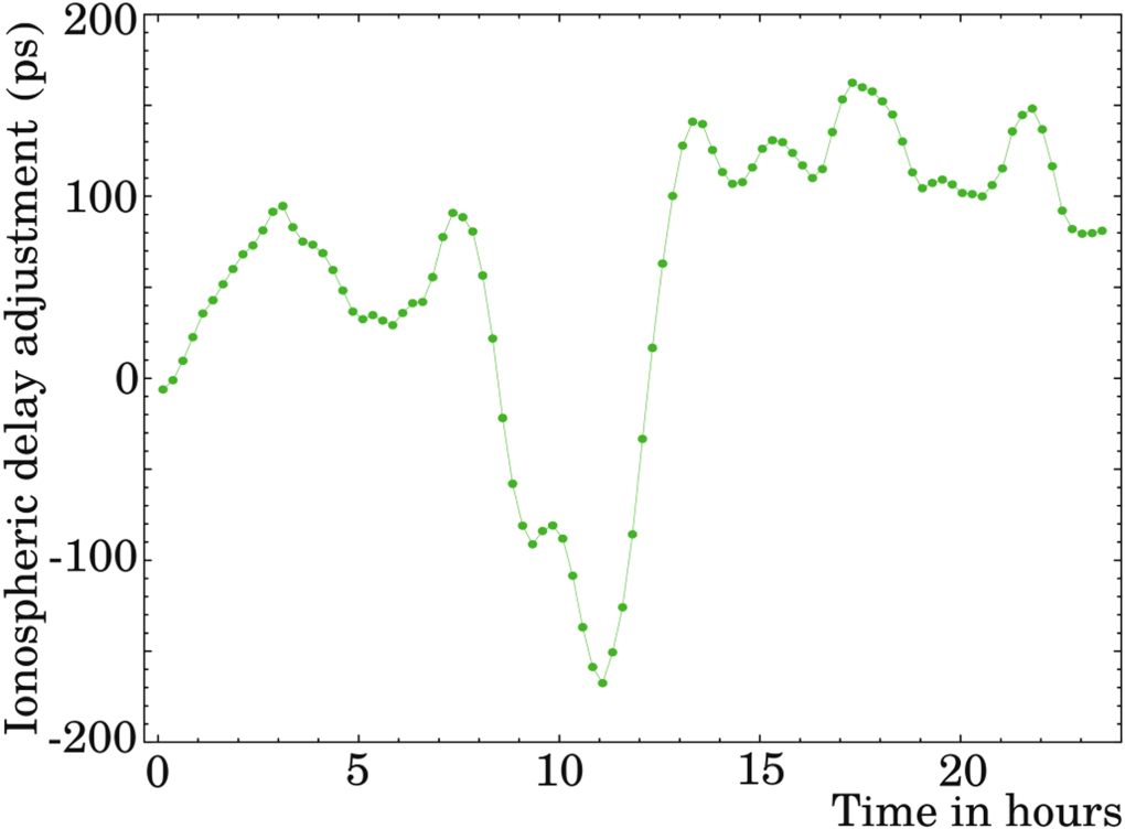
The time span of the B-spline knot sequence for the TEC bias in my solutions was 15 minutes. I applied constraints on the values of the B-spline coefficients and on the first and the second derivatives with the reciprocal weights 5 × 10⁻¹⁰ s, 4 × 10⁻¹⁴, and 2 × 10⁻¹⁸ s−1, respectively. These constraints were introduced to ensure the continuity of biases and to prevent a singularity in rare cases when too few available observations at a given station could be used for bias estimation in a given spline segment. Figure 1 illustrates the estimates of the ionospheric bias.

Figure 1. Adjustment to the ionosphere path delay bias at 8.4 GHz with respect to the path delay derived from GNSS TEC maps at the mk-vlba station from processing dual-band observations on 2015 April 22. The bias estimate corresponds to the averaged positions of the ionosphere piercing points within a given time interval. 1 TECU causes a group delay of 21 ps at 8.4 GHz.
Download figure:
Standard image High-resolution imageThe resulting total electron content model TECj(t) + aj(t) is more precise than the a priori TECj(t) model taken from GNSS maps because it uses additional information. Using estimates of the aj and bj spline coefficients, I compute τi (t) and its uncertainty according to the law of error propagation using the full variance-covariance matrix of the estimated spline coefficients. In order to evaluate the realism of these errors, I processed the trial data set and computed τi (t) using the estimates of the clock and TEC biases and compared them with the ionospheric contribution derived from dual-band observations. I removed clock biases from the VLBI dual-band ionospheric contributions τvi, formed the difference τi − τvi, and then divided them by σ(τi ).
The uncertainty σ(τi ) was derived from the variance-covariance matrix of aj and bj estimates. I generated a normalized histogram from a data set of 4,343,782 differences and computed the first two moments of the empirical distribution shown in Figure 2. The fitting parameters of the first and second moments of the distribution are 0.003 and 0.889, respectively. Two factors cause a deviation of the second moment from 1.0 in the opposite way: (a) TEC variations not accounted for by the parametric model and (b) statistical dependence of the estimates of aj , bj , and the VLBI path delay. After scaling the variance-covariance matrix by the square of 0.889, the distribution of the normalized residuals becomes close to Gaussian. The closeness of the empirical distribution to the normal distribution provides us with confidence that the extra noise introduced by the mismodeled ionospheric path delay after applying clock and TEC biases is properly considered.

Figure 2. Empirical distribution of the normalized differences of the ionosphere path delay computed from the GNSS TEC maps adjusted for clock and TEC biases (green dots). The normal distribution with σ = 1 is shown as a reference (solid blue line).
Download figure:
Standard image High-resolution imageThe closeness of the distribution of the normalized differences to a Gaussian with σ = 1 is encouraging, but it does not guarantee that the residual errors of the sum of the TEC from GNSS and the TEC bias adjustments cause no systematic errors in the estimates of source positions. To characterize the impact of the residual errors of the ionospheric contribution on source position, I ran solution XIA that had the following differences with respect to the reference solution: (1) it used X-band group delays; (2) data reduction for the ionosphere accounted for both a priori TEC from GNSS maps and ionosphere bias adjustment (expression in the parentheses in Equation (8)); and (3) the errors of the ionospheric biases  were added in quadrature to the reciprocal weights of the observables. It should be stressed that the parameterization, editing, and delay uncertainties were exactly the same as in the reference dual-band solution. In all trial solutions I only varied the input observables, changed the ionosphere-specific reduction model, and added noise to the delay uncertainties. Since I analyzed only the differences in the solutions, the contributions of other model deficiencies, such as the path delay in the neutral atmosphere, were canceled when I formed the differences.
I ran also solution SIA that differed from XIA by using S-band group delays and the S-band effective ionospheric frequency fe
. For control, I ran solutions XIN and SIN that used ionosphere-free combinations of the group delays and the same weights as used in the XIA and SIA solutions, respectively, and zero-mean Gaussian noise with  was added to each observable. The differences in the XIA and SIA solutions with respect to the reference solution provide us with a measure of the impact of the residual ionospheric errors on source position. The differences in the XIN and SIN solutions characterize the impact of the residual ionospheric errors if they were Gaussian and totally uncorrelated.
Figure 3 shows the distribution of the differences in the declinations of source position estimates from the XIA and XIN solutions. There is no noticeable deviation from the Gaussian shape. Table 1 lists first two moments of the distribution of the position differences in both right ascension and declination. The second moment from the SIN solution is close to 1.0, while the second moment from the XIN solution is 0.56. The errors of the ionospheric contribution in the S band dominate the error budget. These errors are 14 times less for the X band and are only a fraction of the overall group delay errors. The mean biases in right ascension and declination are negligible. The second moment of the position estimates from the XIA and SIA solutions is 15% higher than the moments from the positions from the XIN and SIN solutions. This increase occurs due to nonrandomness of the residual ionospheric errors and can be viewed as a measure of the unaccounted systematic errors in the source positions due to the ionosphere. Analysis of these trial solutions demonstrates that we are able to predict the impact of the ionospheric errors on source position with an accuracy of 15% when the TEC bias is estimated using dual-band observations.

Figure 3. The distribution of normalized differences in declination from the trial VLBI solutions with respect to the reference dual-band solution. Left: solution with GNSS TEC maps + adjustments of the TEC biases using dual-band VLBI group delays (XIA). Right: solution with added Gaussian noise with σ equal to the errors in the path delay, which correspond to the TEC bias adjustments uncertainties (XIN). The thick blue lines show the fitted Gaussian distributions with the first and second moments listed in Table 1.
Download figure:
Standard image High-resolution imageTable 1. The First and Second Moments of the Position Differences of the Trial Solutions XIA, SIA, XIN, and SIN with Respect to the Position
| Parameter | TEC Biases Adjusted | Gaussian Noise Added | ||
|---|---|---|---|---|
| mean | σ | mean | σ | |
| Δα X- band | −0.03 | 0.63 | −0.01 | 0.56 |
| Δδ X band | 0.02 | 0.64 | 0.01 | 0.56 |
| Δα S band | −0.05 | 1.14 | −0.01 | 1.03 |
| Δδ S band | 0.06 | 1.13 | 0.02 | 1.02 |
Note. The a priori TEC from GNSS and bias adjustment from the dual-band solutions were applied in the XIA and SIA solutions (the second column). Zero-mean Gaussian noise with σ equal to the uncertainty in the path delay from the TEC bias adjustment was added in the XIN and SIN solutions (the third column).
Download table as: ASCIITypeset image
3.4. Ionospheric Contribution in Single-band Observing Sessions
TEC biases cannot be computed when an entire session is observed only in one band. Therefore, we have to resort to deriving a regression model to provide estimates of these errors. In the past, Petrov et al. (2019) derived a regression against the so-called global TEC: the integral of the TEC over the entire Earth, following the ideas of Afraimovich et al. (2008). Later, Krásná & Petrov (2021) derived a regression against a function of the rms of the total ionospheric path delay from GNSS TEC. In this study I use the second approach with slight modifications. Following the general results of turbulence theory (see Tatarskii 1971), we can expect that fluctuations at scale x are related to fluctuations at scale y via a power law.
I processed the same data set of data from 263 24 hr VLBI experiments that were used in the previous section and computed the residual ionospheric path delay for each observation as

where τgi is the vertical ionospheric path delay from GNSS TEC maps, τvi is the vertical ionospheric path delay from VLBI, bj
− bk
are contributions of the clock bias, and  is the averaged ionosphere mapping function between stations 1 and 2 of a given baseline:
  . The clock biases are routinely adjusted during analysis of VLBI observations and therefore their contribution to VLBI results, such as source positions, is entirely eliminated. Subtracting them in Equation (10), I eliminate their impact on the statistics as well. I used only 24 hr VLBI experiments for deriving the statistics because the ionospheric path delay strongly depends on solar time, especially at low latitudes, and the statistics derived for shorter time intervals may not be representative.
Figure 4 shows the dependence of the rms of the residuals τr on the rms of the total ionospheric path delay from the GNSS TEC maps τgi. Each point on the plot corresponds to the rms for a given baseline and a given observing session. I confirm the early result of Krásná & Petrov (2021) but here I used a much larger data set. The result reported in Krásná & Petrov (2021) was slightly affected by an error in computing the ionospheric group delays for a case when some data are flagged because of radio interference. This error has been fixed and the affected experiments have been reprocessed from scratch. This dependence can be coarsely described as the square root of the rms of the total ionospheric path delay. For a better approximation I sought a regression in the form of an expansion over B-splines of the third degree. The spline coefficients computed using least squares are listed in Table 2.

Figure 4. Dependence of the rms of the residual ionospheric path delay derived from GNSS TEC maps σgr on the rms of the total ionospheric path delay from these maps σgt. No adjustment to the TEC has been applied. The path delay is computed for the reference frequency 8 GHz. The blue smooth line shows the regression model in a form of a B-spline that fits the data.
Download figure:
Standard image High-resolution imageTable 2. Coefficients of the B-spline Expansion of the Dependence of the RMS of the Residual Ionospheric Path Delay Derived from GNSS TEC Maps on the RMS of the Total Ionospheric Path Delay from GNSS TEC Maps at 8 GHz
| Knot Index | Knot Argument | B-spline Value |
|---|---|---|
| (ps) | (ps) | |
| −2 | 6.3 | |
| −1 | 14.8 | |
| 0 | 23.5 | |
| 1 | 0.0 | 114.0 |
| 2 | 35.0 | 114.0 |
| 3 | 120.0 | 114.0 |
| 4 | 1300.0 |
Download table as: ASCIITypeset image
Using that regression, I developed the following algorithm for computing the errors of the ionospheric path delay from GNSS TEC maps. First, the coordinates of K points uniformly distributed over the sphere are computed using a random number generator. Then for each baseline and each time epoch, the azimuth and elevation angles of that point are computed at both stations of the baseline, and if the elevations above the horizon are greater than 5° at both stations, that point is selected for further computations. If not, the next point is drawn. Then the total ionospheric path delay τi (A1, e1, A2, e2) is computed using the GNSS TEC maps. It is worth mentioning here that unlike the troposphere path delay, τi (A, e) ≠ τi (A, π/2) × M(e), since the path delay depends on the positions of the ionosphere piercing points. It is not sufficient to compute the ionospheric path delay in the zenith direction and then map it via M(e): latitude and longitude of the piercing point can be as far as 1000 km from the station. Following this approach, we sample piercing points uniformly distributed within the mutual visibility zone. The process is repeated for 1440 time epochs that cover the time interval of the VLBI experiment under consideration with a step of one minute. Then for each baseline σ(τgt) is computed over a time series of 1440 τi values. Finally, the estimate of the rms of residual ionospheric path delay derived from the GNSS TEC maps is computed from this regression via the rms of the total ionospheric path delay as

Baseline-dependent data sets are considered independent for this computation: the mutual visibility at all the stations of the network at a given moment of time is not enforced. For several baselines longer than 96% of Earth's diameter, this algorithm has poor performance for selecting points above 5°. Therefore a minor modification is made for such an extreme case: the elevation angle is fixed to 5°, mutual visibility is not enforced, and azimuths are selected randomly within a range of [0, 2π] independently for both stations.
In order to evaluate the validity of this regression model of the residual ionospheric path delay errors, I computed τr from dual-band observations σgt following the algorithm described above for 263 24 hr experiments, and then computed histograms of the normalized residuals τr /σrr. One such histogram is presented in Figure 5. The first two moments of the distribution are −0.083 and 1.214, respectively. Since regression σrr was found using least squares, the number of observations with σ(τgr) less and greater than σrr for given σ(τgt) is approximately equal; the thick blue line cuts the cloud of green points in Figure 5 almost by half. However, the variance of the contribution of those points with σ(τr ) > σrr overweights the contribution of those points with σ(τr ) < σrr because variance quadratically depends on τr . This causes a positive bias. After multiplying σrr by 1.214, the distribution of normalized residuals becomes almost Gaussian.

Figure 5. The distribution of the normalized differences of the ionospheric path delay computed from the GNSS TEC maps against the VLBI ionospheric path delay with clock biases subtracted (green dots). The normal distribution with σ = 1 (solid blue line) is shown as a reference.
Download figure:
Standard image High-resolution imageOne can notice that  in Equation (11) is not the same as
  used for computation of the regression. I found that using
  instead of
  decreases the second moment from to 1.214 to 1.196, which is negligible,
The distributions shown in Figures 2 and 5 are computed for the entire data set of 4.3 million path delays and they represent the general population over the interval of 23 yr. Statistics for an individual observing session may differ. In order to evaluate the scatter of the statistics, I computed a time series of second moments of the distribution of normalized residuals of ionospheric path delays and their uncertainties with and without TEC biases adjusted for each observing session separately. I divided the normalized residuals by scaling factors of 0.889 and 1.196, respectively. I computed the distribution of second-moment estimates and show it in Figure 6. The scatter of the second moments is small when TEC biases are adjusted. That means these statistics are robust. When TEC is not adjusted, the scatter is significantly larger, but even in that case 90% of the second-moment estimates deviate from 1.0 by no more than 30%. This provides us with a measure of the uncertainties in the computation of ionospheric path delay errors in individual single-band observing sessions.

Figure 6. The distribution of second-moment estimates of the normalized differences of the ionospheric path delays derived from VLBI dual-band observations and GNSS TEC maps among individual observing sessions. The narrow green curve shows the statistics of the normalized residuals with TEC biases adjusted and the wide blue curve show the statistics of the normalized residuals without TEC adjustment.
Download figure:
Standard image High-resolution image3.5. The Impact of the Residual Ionospheric Errors on Source Position in the Case of Single-band Observing Sessions
The error analysis presented in the previous section characterizes our ability to predict the first and second moments of the distribution, but it does not guarantee that the residual errors due to the ionosphere cause no systematic errors in the source positions. I ran trial solutions XIT and SIT that used X- and S-band group delays, respectively, applied ionospheric path delays derived from the GNSS TEC maps, and inflated the reciprocal weights of the observables by adding in quadrature the errors in the ionospheric path delays from the TEC maps.
The analysis of the differences in the source positions from the trial XIT and SIT solutions with respect to the reference dual-band solution revealed no peculiarities in right ascension, but revealed significant systematic errors in declination (see Figure 7). The pattern of systematic errors in declination from the S-band solution is similar but greater by a factor of  . We cannot consider a solution with such errors as satisfactory. This was unexpected because the prior work of Sekido et al. (2003), Hobiger et al. (2006), Dettmering et al. (2011), and Motlaghzadeh et al. (2022) claimed a good agreement between the TEC derived from VLBI and GNSS. And indeed, the plot of the ionospheric contributions in the zenith direction from the VLBI after removal of the clock biases against the ionospheric contributions from GNSS (Figure 8) shows no peculiarities. The least-square approximation of this dependence to the straight line is τvi = −3.9 ps + 1.06 × τgi. Although the residuals of this dependence look random, they still cause systematic errors in source positions.

Figure 7. Differences in declination from the X-band solution XIT using data from the VLBA network with the data reduction for the ionosphere using the ionospheric path delay from the GNSS TEC maps applied with respect to the dual-band reference solution. The thick blue line shows the differences smoothed with a Gaussian filter.
Download figure:
Standard image High-resolution image
Figure 8. Dependence of the VLBI ionospheric group delay at 8 GHz against the ionospheric group delay from GNSS. The blue straight line is the least-squares fit of this dependence.
Download figure:
Standard image High-resolution imageI made a number of trial solutions. The following leads turned out to be productive: (1) to modify the mapping function and (2) to scale the ionospheric path delays from the TEC. Schaer (1999) suggested the following modification of the ionospheric mapping function

arguing that by varying parameters α and Hi one can account for a more realistic electron density distribution with height than a thin-shell model. Here ΔH is an increment in the ionosphere height and α is a fudge factor.
I ran 12 trial solutions with mapping functions with parameters (1) ΔH = 0.0 km, α = 1.0; (2) ΔH = 56.7 km, α = 0.9782; and (3) ΔH = 150.0 km, α = 0.9782. Variant 2 corresponds to the so-called JPL-modified single-layer ionospheric mapping function. It was used in a number of papers (Li et al. 2019; Xiang & Gao 2019; Wielgosz et al. 2021; Zhao et al. 2021), however no details of how these values of k, ΔH, and α were derived have been provided. I varied the mapping function scaling factor k, setting it to 0.7, 0.8, 0.9, and 1.0 and computed declination biases with respect to the reference solution. The results are presented in Figures 9–11.

Figure 9. Smoothed declination biases from four solutions with respect to the dual-band reference solution using X-band observables and the ionospheric mapping function with parameters ΔH = 0, α = 1.0 with different scaling factors k = 0.7, 0.8, 0.9, and 1.0.
Download figure:
Standard image High-resolution image
Figure 10. Smoothed declination biases from four solution with respect to the dual-band reference solution using X-band observables and the ionospheric mapping function with parameters ΔH = 56.7 km and α = 0.9782 with different scaling factors k = 0.7, 0.8, 0.9, and 1.0.
Download figure:
Standard image High-resolution imageThe declination bias is reduced when the parameter ionosphere height in the mapping function is increased. I interpret this result as a deficiency of the GNSS TEC maps and I associate the origin of this deficiency with an oversimplification of the mapping function that was used for derivation of the TEC maps from processing of GNSS observations.
Close analysis of these figures reveals that the declination bias has three components: (1) a constant; (2) a linear increase in the declination bias with a decrease of declination; and (3) the feature  , with the minimum at approximately −12°, where δ is the declination. All three components depend on the parameters of the mapping function, ΔH and α, and on the scaling factor k. Selecting the optimal ΔH, α, k, we can reduce the declination biases. I selected ΔH = 56.7 km, α = 0.9782, and k = 0.85. This choice makes the weighted mean declination bias over all sources 0.013 mas. There is an element of subjectivity in this specific choice, since there exist another combinations of ΔH, α, k that provide a zero mean bias. Wielgosz et al. (2021) showed that the use of the modified mapping function results in a reduction of the mean rms of the difference between GNSS TEC maps and GNSS slant TEC in a range of 2 to 6%. That choice of ΔH and α led me to a selection of the specific scaling factor k.
Although scaling and modification of the ionospheric mapping function results in a substantial reduction of the declination bias, the remaining bias is still worrisome. To mitigate the bias even further, I introduce an ad hoc correction for the ionospheric bias in the data reduction model. I smoothed the biases D(δ) with a Gaussian filter with σ = 8°—these smoothed biases are shown in Figures 9–11—and expanded them over the basis of B-splines of the third degree with 13 equidistant knots in the range of [−45°, 90°]. The expansion coefficients are presented in the Appendix. I added the correction

to the observables. Here fe is the effective ionospheric path delay of a given observation. Figure 12 shows the effect of applying the debias correction. The bias has gone.

Figure 11. Smoothed declination biases from four solutions with respect to the dual-band reference solution using X-band observables and the ionospheric mapping function with parameters ΔH = 150 km and α = 0.9782 with different scaling factors k = 0.7, 0.8, 0.9, and 1.0.
Download figure:
Standard image High-resolution image
Figure 12. The declination with the ionospheric path delay using the mapping function with parameters ΔH = 56.7 km, α = 0.9782, and k = 0.85 with (right) and without (left) applying the empirical debias correction.
Download figure:
Standard image High-resolution imageI ran two solutions using X-band only data (XIB) and S-band only data (SIB), and applied both the a priori ionospheric path delays derived from GNSS TEC maps using the modified mapping function with parameters ΔH = 56.7 km, α = 0.9782, and k = 0.85 and the declination bias correction. The reciprocal weights of the observables were adjusted by adding in quadrature the residual ionospheric errors σrr modeled according to the regression in Equation (11). The first and the second moments of the normalized differences in sources positions are presented in Table 3. The second moments are less than 1.0 in the X-band solution. This indicates that the ionospheric contribution is not the dominant error source in these solutions.
Table 3. The First and Second Moments of the Position Differences of Trial Solutions XIB and SIB with Respect to the Source Position Estimates Derived from the Reference Solution
| Parameter | X-band Solution | S-band Solution | ||
|---|---|---|---|---|
| mean | σ | mean | σ | |
| Δα | −0.07 | 0.45 | −0.11 | 0.82 |
| Δδ | −0.02 | 0.50 | −0.06 | 1.00 |
Note. The a priori ionospheric contribution was computed from the GNSS TEC maps using the modified mapping function with parameters ΔH = 56.7 km, α = 0.9782, and k = 0.85, and the declination bias correction was applied, but no reduction for a TEC bias adjustment has been applied.
Download table as: ASCIITypeset image
Unfortunately, it does not look possible to fix the deficiency of the GNSS TEC maps without reprocessing the GNSS observations, which is well beyond the scope of this article, but nevertheless, it is still feasible to mitigate the impact of the imperfection of GNSS TEC maps on source position estimates.
4. Discussion
4.1. Inaccuracy of GNSS TEC Maps
A number of authors compared the ionospheric contribution from GNSS, VLBI, DORIS, radio occultation observations, and dual-band satellite altimeters (Sekido et al. 2003; Hobiger et al. 2006; Dettmering et al. 2011; Hernández-Pajares et al. 2017; Cokrlic et al. 2018; Li et al. 2018, 2019; Xiang & Gao 2019; Wielgosz et al. 2021; Zhao et al. 2021; Motlaghzadeh et al. 2022). A message these publications convey is there is a reasonable agreement between GNSS TEC maps and other techniques and there are no majors problems. Therefore, large systematic errors driven by mismodeling of the ionospheric contribution derived from GNSS maps came as a surprise. Do the results presented in this study contradict those of the prior publications?
Comparison in the past was often performed using very short continuous data sets of VLBI observations, from 5 to 15 days (Hobiger et al. 2005; Dettmering et al. 2011; Etemadfard et al. 2021; Motlaghzadeh et al. 2022). The level of agreement was characterized in terms of additive errors in the GNSS TEC model. Unfortunately, when data from a short time interval are analyzed, a distinction between additive and multiplicative errors becomes blurry. Characterizing the differences in terms of biases and rms of their scatter did not turn out productive in revealing systematic errors. Moreover, an unconscious bias of focusing a study on the assessment of an agreement rather than investigation of disagreements, which were noticed and just briefly reported, diverted attention from investigating the differences in depth.
However, reading between the lines of the published papers, we can find pieces of evidence supporting the findings in this work. The distribution of differences in the VLBI vertical TEC with respect to the TEC derived from GNSS TEC maps presented in Figure 6 in Hobiger et al. (2006) shows a very significant skew. The distribution has a negative mean and a much greater left tail than a right tail. The VLBI vertical TEC from that study appeared less than the TEC from the GNSS TEC maps, in agreement with what I have found. The authors did not investigate that stark deviation of the distribution of over one million differences from the Gaussian shape, only noting that the bias is less than 3 TECU. Considering the errors are normally distributed and additive, and considering that the derivation of the TEC from the VLBI does not introduce serious errors, one can expect to arrive to a Gaussian distribution of the residuals. For instance, the distribution of differences in Figure 5 indeed does not show any measurable deviation from a Gaussian shape. However, if the errors are multiplicative, the residuals will be non-Gaussian and their distribution will be skewed.
Satellite altimetry using Jason satellites (Vaze et al. 2010, and references therein) provides an independent way for assessing the level of disagreement between direct vertical TEC measurements and GNSS TEC maps. Li et al. (2018) showed that comparisons of the differences revealed significant systematic biases that depend on geomagnetic latitude. However, an attempt to characterize these additive biases in terms of the rms was not very productive. Liu et al. (2018) presented the spatial distribution of the differences (their Figures 6–7). That distribution strikingly reminds us of the average distribution of the TEC itself, suggesting the differences are multiplicative. The more recent paper of Dettmering & Schwatke (2022) revealed a highly significant scaling factor between GNSS TEC maps and four altimeter missions. The scaling factors estimated separately from the analysis of these four missions varied from 0.809 to 0.919, which are very close to what has been found in my analysis of astrometric observations of extragalactic radio sources.
Li et al. (2019) performed a comparison of TEC maps with Jason satellite altimetry and with ionospheric radio occultations (see the overview of this technique in Bonafoni et al. 2019). They characterized the differences as the superposition of an additive bias and a multiplicative scale factor. The scale factors defined as TEC and TECCOSMIC/TEC
 vary with time and latitude and stay in a range of 0.7–0.9 at night and 0.9–1.0 during the daytime. Since Jason orbits have an altitude of 1350 km and GNSS orbits have an altitude of about 20,000 km, Jason altimetry misses the contribution from the upper layers of the ionosphere and the plasmasphere. Yizengaw et al. (2008) analyzed the TEC between the Jason and GNSS satellites and found that the share of plasmasphere to the TEC is on average 15% and may reach 60% when the TEC is low. However, such a large share of the electron density at altitudes above 1350 km is inconsistent with the thin-shell model at altitudes of 450 or 506.7 km, which assumes no electron density above that height at all.
It is essential to note that the analysis of Jason and COSMIC data provides estimates of the vertical TEC, while the analysis of GNSS observations provides the slant TEC that is converted to the vertical TEC using a mapping function. The dependence of the declination biases on the mapping function found in this study suggests that a simple thin model may not be adequate. Schaer (1999) discussed the dependence of the effective ionosphere height on the solar zenith angle. Xiang & Gao (2019) studied it in more detail. The height of the peak electron density has annual and diurnal variations. The latter variations have an amplitude of about 100 km, being lower at daytime. They showed that the instantaneous mapping function that accounts for the height of the electron content maximum achieves a 8% reduction of mapping errors. It should be mentioned that if the effective height of the ionosphere is changed, the latitude and longitude of the ionosphere piercing point for an observation with a given elevation and azimuth will change as well, which will provide an additional change in the path delay.
These works strengthen argumentation in favor of that the thin-shell model used for the derivation of TEC maps since the mid-1990s is oversimplified. The effective height of the ionosphere changes with time and latitude and therefore, a realistic mapping function should also vary with time and latitude. Omission of this complexity results in a deficiency of GNSS TEC maps that manifests in multiplicative (scale) and additive (bias) errors that vary with time and latitude. The nonlinear dependence of the declination bias with declination in the form of  may be caused by the dependence of the GNSS TEC scaling factor on latitude, reported by Li et al. (2019). Radio waves from Southern Hemisphere sources observed at the array located in the Northern Hemisphere propagate through regions in the ionosphere with systematically lower latitudes than from Northern Hemisphere sources. Since a fixed mapping function is used for both computation of TEC maps and computation of the slant ionospheric path delay from these maps, no modification of that fixed mapping function for the data reduction of astronomical data is able to account for this kind of complexity, but as it was shown earlier, it is still possible to mitigate it. The remaining bias can be eliminated by applying the empirical debias correction.
4.2. Omitted Refinements of the Ionosphere Contribution
Etemadfard et al. (2021) processed 60 days of VLBI data and estimated not only the TEC for each site using B-splines of the first degree, but also TEC derivatives over longitude and latitude that were considered constant over 24 hr periods. They claim that estimating TEC partial derivatives decreases the discrepancies of the TEC from VLBI to GNSS TEC maps by 36%. Inspired by this result, I introduced estimation of the latitude and longitude TEC gradients in the form of a B-spline in addition to TEC estimation using dual-band data. I considered the weighted rms (wrms) of the differences between the parameterized model of the TEC adjustment to the vertical TEC from dual-band data as a metric of improvement. I did not find a reduction of the rms greater than several percent and abandoned this approach. I should note this result does not disprove the findings of Etemadfard et al. (2021) since they used a different metric.
Expression for the ionospheric contribution (Equation (1)) is an approximation. Hawarey et al. (2005) considered the impact of a higher-order expansion on the group delay, namely proportional to f−3. They found that the maximum contribution of the third degree term varied from 3 to 9 ps at 8 GHz, depending on the baseline. This contribution is approximately one order of magnitude less than the contribution of the residual ionospheric errors after taking into account the GNSS TEC maps. It should be noted that the third degree term affects both single-band and ionosphere-free linear combinations of the group delays in two bands and therefore, cannot be retrieved in an analysis of the differences with respect to the dual-band reference solution.
4.3. The Impact of the Remaining Errors in Modeling the Ionosphere on Source Position
As it was shown before, our ability to model the ionospheric contribution using single-band observations is limited. After applying the declination debias in the data reduction procedure, the declination bias is virtually eliminated. The residual ionospheric contribution causes additional random errors. In order to investigate their impact, I ran four trial solutions. I used ionosphere-free linear combinations of dual-band data and added to them the ionospheric contribution derived from VLBI data scaled to the specific frequency of the trial solution. I computed the contribution of the ionospheric path delay for modified observables using the GNSS TEC maps as if I processed single-band observations and then I estimated source positions. The differences in the source positions from these solutions with respect to the reference solutions are interpreted as the impact of the residual ionospheric errors at different frequencies. The declination dependence of the differences in right ascension and declination for four solutions at frequencies 2.3 GHz (S band), 4.3 GHz (C band), 8.4 GHz (X band), and 23.7 GHz (K band) is shown in Figure 13.

Figure 13. The rms of the differences in right ascension (upper row) and declination (lower row) when single-band group delays are used with respect to the positions from the dual-band reference solution. The a priori ionospheric path delay using GNSS TEC with the modified mapping function (ΔH = 56.7 km, α = 0.9782, and k = 0.85) was used by adjusting the TEC biases from the dual-band observations (right) and without adjusting the biases but with applying the debias correction from Equation (13), shown in the left column. The upper blue band shows the differences for S band, the next red line shows the differences for C band, the next green line shows the differences for X band, and the bottom purple line shows the differences for K band.
Download figure:
Standard image High-resolution imageThese plots help to quantify the additional errors in source positions that would arise if the data set of data from 263 24 hr experiments used for this study would have been observed in one band only. We see that estimation of the TEC biases reduces the ionosphere-driven errors by a factor of 2–4. Still, even after estimation of the TEC biases, the declination dependence of the ionosphere-driven errors remains.
It is known that unaccounted source structure affects source position estimates. In general, the contribution of source structure at higher frequencies is less because jets become optically thin. Therefore, there was an expectation that observing at high frequencies, such as 22–24 GHz (K band), one may obtain more precise source positions. So far, observational evidence do not support that prediction (Lanyi et al. 2010; Charlot et al. 2020). A detailed comparison of the K-band absolute astrometry versus dual-band astrometry of Karbon & Nothnagel (2019) did not reveal an improvement. Therefore, it is instructive to see what is the contribution of the ionospheric errors in K band after applying data reduction from the GNSS TEC maps. Figure 14 shows the additional errors in right ascension and declination due to the residual contribution of the ionosphere. We see that the additional errors in right ascension are about 0.1 mas. Declination errors of Northern Hemisphere sources are at the same level. However, these errors grow with a decrease of declination for sources in the Southern Hemisphere approximately linearly and reach 0.3 mas at a decl. of −40°. Therefore, the unmodeled ionospheric contribution sets the error floor in position accuracy. This error floor is not accounted for in the ICRF3 catalog, and the unaccounted ionospheric contribution is 300% greater than the noise floor in K band adopted by Charlot et al. (2020) according to their Table 6. The potential of K-band astrometry cannot be utilized unless the accuracy of ionosphere modeling will be substantially improved.

Figure 14. An increase in source position errors in right ascension (left) and declination (right) due to the residual ionospheric contribution in K band (22 GHz) after applying data reduction based on the GNSS TEC maps with the modified mapping function (ΔH = 56.7 km, α = 0.9782, and k = 0.85).
Download figure:
Standard image High-resolution image4.4. The rms of the Residual Atmospheric Errors
I investigated how the rms of the residual ionospheric contribution for 45 VLBA baselines from the data set of data from 263 24 hr observing sessions varied with time. I computed three statistics for each observing session: (1) τv − bi , (2) τv − τg − bi, and (3) τv − τg − ai − bi , and rescaled them to 8 GHz. Here τv and τg are the ionospheric path delays from VLBI and TEC maps respectively, ai is the adjusted TEC bias, and bi is the clock bias. The statistics are shown in Figure 15. In order to improve readability, the time series was smoothed using a Gaussian kernel with parameter σ = 1 yr. The first statistic characterizes the impact of the total ionosphere on the group delay. The second statistic characterizes the rms of the impact of the residual ionospheric errors on the group delay after applying the a priori GNSS TEC model. The final statistic characterizes the impact of the residual errors after applying the a priori GNSS TEC and adjusting the TEC biases using dual-band VLBI data.

Figure 15. The rms of the mean residual ionospheric contribution at VLBA baselines at 8 GHz for three cases: (1) no a priori ionospheric contribution is applied (upper red curve); (2) the a priori ionospheric path delay computed using GNSS TEC maps is applied (middle blue curve); and (3) the a priori ionospheric path delay computed using GNSS TEC maps are applied and the TEC biases are adjusted (lower green curve). 1 TECU causes a group delay of 21 ps at 8 GHz.
Download figure:
Standard image High-resolution image4.5. Processing Geodetic Data from Southern and R1/R4 VLBI Experiments
It would be instructive to explore to which extent the numerical values found in processing data from the VLBA network are representative to experiments conducted at other VLBI networks and to which extent they are specific to VLBA. I ran two solutions, XIS and XIR. Solution XIS used 63,984 X-band group delays from 36 VLBI experiments in 2016–2019 for absolute astrometry programs at core Southern Hemisphere stations hart15m, hartrao, hobart12, hobart26, kath12m, tidbin64, wark12m, and yarra12m with participation of other International VLBI Service for geodesy (IVS) stations. Solution XIR used 6,600,959 X-band group delays from 2154 geodetic VLBI experiments from IVS programs R1 and R4 (Lambert & Gontier 2006) for 2002–2022. Data from R1, R4, and Southern Hemisphere VLBI experiments are available at the NASA Crustal Dynamic Data Information System. 2 In total, 36 globally distributed stations participated in experiments under R1 and R4 programs. These experiments were designed for Earth orientation parameter determination. I computed also reference solutions RIS and RIR that used ionosphere-free combinations of dual-band group delays. Solution parameterization and editing were identical for pairs of XIS/RIS and RIS/RIR solutions.
I compared the source positions from the XIS/RIS and XIR/RIR solutions. In both cases systematic declination errors are evident. I found that scaling that makes the mean declination bias of the XIS solution close to zero is k = 0.78, somewhat smaller than that from solution XIB based on data from the VLBA network. Moreover, estimates of the declinations from the XIS solution require a different debias correction than declinations from the XIB solution.
Figure 16 shows the differences in declination from position estimates of 638 sources with formal uncertainties <0.5 mas from the XIR solution with respect to the reference solution RIR based on data from the R1/R4 networks. Comparing solutions made with different values of the mapping function parameter k, I found that the mean declination bias vanishes when k = 0.75. The shape of the bias and its magnitude is noticeably different than the bias from declinations derived using the group delays from observations at the VLBA network (see Figure 7).

Figure 16. Differences in declination from the X-band solution XIR with respect to the dual reference solution RIR using data from the R1/R4 VLBI, similar to Figure 7. The default TEC GNSS mapping function (ΔH = 0, α = 1.0, and k = 1.00) was used for this comparison.
Download figure:
Standard image High-resolution imageThe magnitude of the peak-to-peak declination bias from the solution that uses data from the R1/R4 network is 0.62 mas, while the magnitude of the declination bias from the solution that uses data from the VLBA network is 0.85 mas. The regional VLBA network stretches over 90° in longitude, but only within [18°, 48°] in latitude, while the global R1/R4 network stretches over all longitudes and over [−43°, +79°] in latitude. Observations of Southern Hemisphere sources with VLBA are possible in southern sectors only, and the further south a source, the lower the elevation that can be observed. At the same time, a given source can be observed at different azimuths and elevations in a global network.
Figure 17 shows the rms of the mean residual ionospheric contribution at R1/R4 baselines. Comparing it with a similar plot for the VLBA network (Figure 15), we see that the wrms of the ionospheric contribution observed in the VLBA network is a factor of 2–3 lower. This can be explained by both differences in the total ionospheric path delay sensed by the stations in the two networks, and by the amount of the ionospheric path delay that is absorbed in the estimates of the parameters, such as the source declination, causing biases. If a source is observed only at a given azimuth and elevation, most of the ionospheric path delay will be absorbed by the estimated parameters that reduce the residuals. The wider spread in azimuth and elevation a given source is observed, the smaller the share of the ionospheric path delay that will be absorbed by the estimated parameters and propagate to the residuals.

Figure 17. Similar to Figure 15 but derived from an analysis of observations from the R1/R4 VLBI network. The statistics are computed for one year intervals.
Download figure:
Standard image High-resolution imageWe can estimate the scaling factor directly from single-band VLBI data using least squares. I ran twelve solutions using data from the VLBA, southern, and R1/R4 networks separately and using data from all three networks altogether and applying three different flavors of the ionospheric mapping function, ΔH = 0, α = 1.0; ΔH = 56.7, α = 0.9782; and ΔH = 150, α = 0.9782. Table 4 displays the estimates. The differences between the estimates of the scaling factors derived from the observations at the R1/R4 and Southern Hemisphere networks are statistically insignificant, while the scaling factor estimates from the VLBA network are systematically lower, and these differences with respect to the R1/R4 network are statistically significant. It is also remarkable that the scaling factors that minimize the postfit residuals differ from those that eliminate the mean declination bias. This implies that scaling does not eliminate systematic errors due to any deficiency of the GNSS TEC maps, but only alleviates their impact.
Table 4. Estimates of the Scaling Factors from Twelve Solutions in the Southern Hemisphere, VLBA, and R1R4 Networks, as well as all Networks Combined
| Network | Ionospheric Mapping Functions | ||
|---|---|---|---|
| (1) | (2) | (3) | |
| VLBA | 0.750 ± 0.002 | 0.801 ± 0.002 | 0.835 ± 0.002 |
| R1R4 | 0.789 ± 0.001 | 0.844 ± 0.001 | 0.882 ± 0.001 |
| South | 0.79 ± 0.02 | 0.84 ± 0.02 | 0.87 ± 0.02 |
| all | 0.780 ± 0.001 | 0.834 ± 0.001 | 0.872 ± 0.001 |
Note. Three different ionospheric mapping functions were used: 1: ΔH = 0 m, α = 1.0, k = 1.00; 2: ΔH = 56.7 m, α = 0.9782, k = 1.00; and 3: ΔH = 150 m, α = 0.9782, k = 1.00.
Download table as: ASCIITypeset image
4.6. The Combined Use of Dual-band and Single-band Data
Negligible remaining biases and the realistic assessment of errors due to the residual ionospheric contribution allows us to use a mixture of dual-band and single-band group delays in a single least-square solution. Source positions derived from single-band data are in general less precise than those derived from dual-band data because an additional factor affects the uncertainties of group delays. These additional errors can be computed and accounted for in deriving the weights of observables. An increase in the uncertainties of group delay observables propagates to the uncertainties of source positions.
A combined analysis of a heterogeneous data set provides a significant advantage because all the data are used. We can fuse dual-band and single-band data in one data set and use it for estimation of source positions. A fused data set consists of observables of three types:
- 1.Dual-band ionosphere-free linear combinations of group delays.
- 2.Single-band delays of dual-band experiments detected in one band only. Data reduction accounts for the ionospheric path delay computed from the sum of the GNSS TEC and TEC bias adjustments. The uncertainty of the bias adjustment is added in quadrature to the group delay uncertainty for the reciprocal weights of such observables.
- 3.Group delays from single-band experiments. Data reduction accounts for the ionospheric path delay computed from GNSS TEC and applies the debias correction. The uncertainty of the ionospheric model computed from the regression model is added in quadrature to the group delay uncertainty used for computation of the weights of such observables.
Solving for source coordinates using a fused data set provides estimates with minimum uncertainties and minimum correlations between right ascension and declination since it uses all available data provided the frequency-dependent position biases due to source structure are negligible. This condition may be violated for some strong sources with significant structure. An analysis of positional offsets between single-band and dual-band solutions will help to identify such sources (see, for example, Petrov et al. 2011), but these cases are encountered infrequently.
4.7. Future Work
An improvement in modeling the ionospheric path delay when TEC biases are adjusted is quite impressive. However, this requires using additional information about the state of the ionosphere. Specifically, VLBI ionospheric path delays from dual-band data were used for computation of these biases. This information is not available for processing single-band observations. Ros et al. (2000) considered the use of dual-band GPS observations from collocated receivers for analysis of radio astronomy observations. They have shown that the GPS determination of the TEC from ground receivers alone without the use of GNSS TEC maps can be successfully applied to the astrometric analysis of VLBI observations.
There are ongoing efforts to install advanced GNSS receivers within a hundred meters of each VLBA antenna. The use of geometry-free pseudo-ranges at 1.2 and 1.5 GHz in a similar way as I used VLBI ionosphere-free group delays for adjustments of TEC biases promises a similar level of improvement.
5. Conclusions
Single-band group delays are affected by a contribution from the ionosphere. This contribution is noticeable at frequencies below 30 GHz and becomes a dominant error source at frequencies below 5–8 GHz. Compared with astrometric solutions based on the use of the ionosphere-free linear combinations of dual-band observables, source position estimates derived from a single-band solution are affected by additional random and systematic errors caused by mismodeling the contribution of the ionosphere to path delay. I explored two approaches to modeling the ionospheric path delay using GNSS TEC maps and assessed residual ionospheric errors.
The findings can be summarized as follows:
- 1.In the case when an experiment was recorded in two widely separated bands, but a fraction of sources were detected in one band only, estimation of the TEC bias in the form of an expansion over the B-spline basis using dual-band data and then applying that bias to GNSS TEC maps provides an unbiased estimate of source position. The stochastic model that describes the residual errors of TEC bias adjustment predicts an increase of positional error with an accuracy of 15%. No remaining systematic errors were found. This approach provides source positions with the lowest uncertainties with respect to other approaches.
- 2.In the case of single-band observations, path delays are computed using GNSS TEC maps. The thin spherical shell model of the ionosphere with a constant height of 450 km above the mean Earth radius causes a strong systematic bias in declination that reaches 1 mas at 8 GHz and 12 mas at 2.3 GHz. This bias can be virtually eliminated when (a) the modified ionospheric mapping function with parameters of ΔH = 56.7 km, α = 0.9782, k = 0.85 is used; and (b) an empirical debias correction is applied.
- 3.Ionospheric errors are mainly multiplicative.
- 4.I determined the scaling factor of the TEC from GNSS maps by processing from 11,457,749 VLBI observations at different networks for 25 yr: 0.834 ± 0.001. This estimate is in good agreement with a totally independent comparison of the vertical TEC determined from satellite altimetry against GNSS TEC maps. Since VLBI is sensitive to a delay that incurred in the total ionosphere, interpretation of a scaling factor of TEC from altimetry and radio occultation observations as the contribution of upper layers of the ionosphere at altitudes above Jason orbit, i.e., 1350 km, suggested by Liu et al. (2018) and Dettmering & Schwatke (2022, 2023) is not consistent with presented results. Although the plasmasphere above 1350 km may contribute to discrepancies between Jason and GNSS TEC, systematic errors in GNSS TEC due to the adopted model of the vertical distribution of the electron density in a form of a thin shell at heights of 450 or 506.7 km is another major factor. The contribution of the plasmasphere alone cannot explain the scaling factor.
- 5.I have found that the scaling factor of the GNSS TEC maps that provides a zero mean declination bias depends on the used ionospheric mapping function. Therefore, I surmise that the established deficiency of GNSS TEC maps is caused by oversimplification of the ionospheric mapping function used for their derivation that considers the ionosphere as a thin spherical shell. The electron content in the real ionosphere varies not only in latitude and longitude, but also in height. Diurnal variations of the effective ionosphere height at a level of 100 km, i.e., over 20%, are large enough to cause errors of the magnitude that was found in analysis of VLBI data.
- 6.The impact of the ionosphere on the path delay depends on the solar cycle. Modeling the ionospheric path with GNSS TEC maps reduces the residuals at 8 GHz by a factor of 2 during solar maximum and only by 10% during solar minimum. Estimation of the TEC bias reduces the ionospheric errors further by a factor of 2 regardless of the phase of solar maximum.
- 7.The impact of the ionosphere on source position errors can be modeled with an accuracy of 15%. It remains noticeable even at frequencies as high as 22–24 GHz (K band). In particular, the ionospheric errors even after applying data reduction based on GNSS TEC maps with the modified mapping function and the debias correction exceed 0.1 mas. Declination errors of Southern Hemisphere sources observed with VLBA are in the range of 0.1–0.3 mas. An assertion that K-band astrometry is able to provide results more precise than 0.1 mas is not true at the current state of our ability to model ionospheric path delay. Considering ongoing efforts to install advanced GNSS receivers in the close vicinity of VLBA stations and other radio telescopes, the situation may change in the future.
This study lays the foundation of single-band absolute astrometry. Dual-band astrometric observations still provide the best accuracy. The use of single-band data with the procedure of data reduction and weighting described above allows us to get unbiased positions with known added errors.
This work was done with data sets RDV, RV, CN, UF001, UG003, BL122, BL166, BP133, BP138, GC073, BC204, BG219, and V17 collected with the VLBA instrument of the NRAO and available at https://archive.nrao.edu/archive. The NRAO is a facility of the National Science Foundation operated under cooperative agreement by Associated Universities, Inc. The author acknowledges use of the VLBA under the USNO's time allocation for some data sets. This work made use of the Swinburne University of Technology software correlator, developed as part of the Australian Major National Research Facilities Programme and operated under license. This work was supported by NASA's Space Geodesy Project.
It is my pleasure to thank Yuri Y. Kovalev, Urs Hugentobler, Robert Heinkelmann, Minghui Xu, and Denise Dettmering for discussions of the presented results.
Facility: VLBA - Very Long Baseline Array.
Software: PIMA.
Appendix
Coefficients of the expansion of the empirical correction of the declination bias into the B-spline basis of the third degree due to deficiency of TEC GNSS maps for three networks are given in Table 5. Plots of the empirical corrections D(δ) computed using these coefficients are shown in Figure 18.

Figure 18. The empirical declination bias corrections D(δ) computed from the coefficients presented in Table 5 for three VLBI networks: the Southern Hemisphere network marked with S (red), R1/R4 marked with R (blue), and VLBA marked with V (green).
Download figure:
Standard image High-resolution image
Table 5. Coefficients of the Expansion of the Declination Correction for three Networks into the B-spline Basis of the Third Degree
| VLBA Network | ||
|---|---|---|
| ΔH = 56.7 km, α = 0.9782, k = 0.85 | ||
| knot | δ | Dk (δ) |
| rad | s−2 | |
| −2 | −0.78539 | 1.7254 · 10+11 |
| −1 | −0.78539 | 1.6909 · 10+11 |
| 0 | −0.78539 | 1.1094 · 10+11 |
| 1 | −0.78539 | −1.2356 · 10+10 |
| 2 | −0.58904 | −4.7934 · 10+10 |
| 3 | −0.39269 | −3.3498 · 10+10 |
| 4 | −0.19634 | −4.9275 · 10+09 |
| 5 | 0.00000 | 2.5485 · 10+10 |
| 6 | 0.19634 | 2.2408 · 10+10 |
| 7 | 0.39269 | −1.2769 · 10+09 |
| 8 | 0.58904 | −1.9056 · 10+10 |
| 9 | 0.78539 | −4.3368 · 10+10 |
| 10 | 0.98174 | −3.8566 · 10+10 |
| 11 | 1.17809 | −2.5999 · 10+10 |
| 12 | 1.37444 | −2.3141 · 10+10 |
| 13 | 1.57079 | −2.3141 · 10+10 |
| Southern Network | ||
|---|---|---|
| ΔH = 56.7 km, α = 0.9782, k = 0.78 | ||
| knot | δ | Dk (δ) |
| rad | s−2 | |
| −2 | −1.57079 | 1.4031 · 10+10 |
| −1 | −1.57079 | 1.8702 · 10+10 |
| 0 | −1.57079 | 3.1684 · 10+10 |
| 1 | −1.57079 | 1.7161 · 10+10 |
| 2 | −1.34639 | −1.8306 · 10+10 |
| 3 | −1.12199 | −4.6113 · 10+10 |
| 4 | −0.89759 | −6.3192 · 10+10 |
| 5 | −0.67319 | −4.2758 · 10+10 |
| 6 | −0.44879 | −1.7912 · 10+10 |
| 7 | −0.22439 | −3.2968 · 10+09 |
| 8 | 0.00000 | 3.8267 · 10+10 |
| 9 | 0.22439 | 9.8592 · 10+10 |
| 10 | 0.44879 | 2.5145 · 10+10 |
| 11 | 0.67319 | −1.9324 · 10+10 |
| 12 | 0.89759 | −1.3308 · 10+10 |
| 13 | 1.12199 | 9.5708 · 10+10 |
| 14 | 1.34639 | 8.4468 · 10+10 |
| 15 | 1.57079 | 8.4468 · 10+10 |
| R1/R4 Network | ||
|---|---|---|
| ΔH = 56.7 km, α = 0.9782, k = 0.75 | ||
| knot | δ | Dk (δ) |
| rad | s−2 | |
| −2 | −1.57079 | 4.2459 · 10+10 |
| −1 | −1.57079 | 2.4792 · 10+10 |
| 0 | −1.57079 | 2.8538 · 10+10 |
| 1 | −1.57079 | −7.0868 · 10+09 |
| 2 | −1.34639 | −4.3644 · 10+10 |
| 3 | −1.12199 | −2.8135 · 10+10 |
| 4 | −0.89759 | −3.7050 · 10+10 |
| 5 | −0.67319 | −3.5487 · 10+10 |
| 6 | −0.44879 | −6.1013 · 10+10 |
| 7 | −0.22439 | 9.6720 · 10+09 |
| 8 | 0.00000 | 4.5049 · 10+10 |
| 9 | 0.22439 | 3.7563 · 10+10 |
| 10 | 0.44879 | 1.0745 · 10+09 |
| 11 | 0.67319 | −2.2499 · 10+10 |
| 12 | 0.89759 | −1.3549 · 10+10 |
| 13 | 1.12199 | −5.1436 · 10+09 |
| 14 | 1.34639 | 2.6590 · 10+09 |
| 15 | 1.57079 | 2.6590 · 10+09 |