


Abstract
Kepler 1627A is a G8V star previously known to host a 3.8 R⊕ planet on a 7.2 day orbit. The star was observed by the Kepler space telescope because it is nearby (d = 329 pc) and it resembles the Sun. Here, we show using Gaia kinematics, TESS stellar rotation periods, and spectroscopic lithium abundances that Kepler 1627 is a member of the  Myr old δ Lyr cluster. To our knowledge, this makes Kepler 1627Ab the youngest planet with a precise age yet found by the prime Kepler mission. The Kepler photometry shows two peculiarities: the average transit profile is asymmetric, and the individual transit times might be correlated with the local light-curve slope. We discuss possible explanations for each anomaly. More importantly, the δ Lyr cluster is one of ∼103 coeval groups whose properties have been clarified by Gaia. Many other exoplanet hosts are candidate members of these clusters; their ages can be verified with the trifecta of Gaia, TESS, and ground-based spectroscopy.
Export citation and abstract BibTeX RIS

Original content from this work may be used under the terms of the Creative Commons Attribution 4.0 licence. Any further distribution of this work must maintain attribution to the author(s) and the title of the work, journal citation and DOI.
1. Introduction
While thousands of exoplanets have been discovered orbiting nearby stars, the vast majority of them are several billion years old. This makes it difficult to test origin theories for the different families of planets, since many evolutionary processes are expected to operate on timescales of less than 100 million years.
For instance, the "mini-Neptunes," thought to be made of metal cores, silicate mantles (Kite et al. 2020), and extended hydrogen-dominated atmospheres, are expected to shrink in size by factors of several over their first 108 yr. Specifically, in the models of Owen & Wu (2016) and Owen (2020), the ≈5 M⊕ planets start with sizes of 4–12 R⊕ shortly after the time of disk dispersal (≲107 years), and shrink to sizes of 2–4 R⊕ by 108 yr. While the majority of this change is expected to occur within the first few million years after the disk disperses (Ikoma & Hori 2012), stellar irradiation and internal heat can also power gradual outflows which, if strong enough, can deplete or entirely strip the atmosphere (Lopez et al. 2012; Owen & Wu 2013; Ginzburg et al. 2018). The photoevaporative and core-powered outflows are thought to persist for ≈108 to ≈109 yr, though the details depend on the planetary masses, the irradiation environments, and the initial atmospheric mass fractions (Owen & Wu 2017; Gupta & Schlichting 2020; King & Wheatley 2021; Rogers & Owen 2021). Discovering young planets, measuring their masses, and detecting their atmospheric outflows are key steps toward testing this paradigm, which is often invoked to explain the observed radius distribution of mature exoplanets (Fulton et al. 2017; Van Eylen et al. 2018).
The K2 and TESS missions have now enabled the detection of about 10 close-in planets younger than 100 million years, all smaller than Jupiter (David et al. 2016, 2019; Mann et al. 2016; Newton et al. 2019; Bouma et al. 2020; Plavchan et al. 2020; Rizzuto et al. 2020; Martioli et al. 2021). The Kepler mission however has not yielded any planets with precise ages below one gigayear (Meibom et al. 2013; Cody et al. 2018). The reason is that during the prime Kepler mission (2009–2013), only four open clusters were known in the Kepler field, with ages spanning 0.7 Gyr to 9 Gyr (Meibom et al. 2011). Though isochronal, gyrochronal, and lithium-based analyses suggest that younger Kepler planets do exist (Walkowicz & Basri 2013; Berger et al. 2018; David et al. 2021), accurate and precise age measurements typically require an ensemble of stars. Fortunately, recent analyses of the Gaia data have greatly expanded our knowledge of cluster memberships (e.g., Cantat-Gaudin et al. 2018; Zari et al. 2018; Kounkel & Covey 2019; Kerr et al. 2021; Meingast et al. 2021). As part of our Cluster Difference Imaging Photometric Survey (CDIPS; Bouma et al. 2019), we concatenated the available analyses from the literature, which yielded a list of candidate young and age-dated stars (see Appendix A).
Matching our young star list against stars observed by Kepler revealed that Kepler observed a portion of the δ Lyr cluster (Stephenson-1; Theia 73). More specifically, a clustering analysis of the Gaia data by Kounkel & Covey (2019) reported that Kepler 1627 (KIC 6184894; KOI 5245) is a δ Lyr cluster member. Given the previous statistical validation of the close-in Neptune-sized planet Kepler 1627b (Tenenbaum et al. 2012; Morton et al. 2016; Thompson et al. 2018), we begin by scrutinizing the properties of the cluster (Section 2). We find that the δ Lyr cluster is  Myr old, and in Section 3 we show that Kepler 1627 is both a binary and also a member of the cluster. Focusing on the planet (Section 4), we confirm that despite the existence of the previously unreported M3V companion, hereafter Kepler 1627B, the planet orbits the G-dwarf primary, Kepler 1627A. We also analyze an asymmetry in the average transit profile and a possible correlation between the individual transit times and the local light-curve slope. We conclude by discussing broader implications for our ability to age-date a larger sample of planets (Section 5).
2. The Cluster
To measure the age of the δ Lyr cluster, we first selected a set of candidate cluster members (Section 2.1), and then analyzed these stars using a combination of the isochronal and gyrochronal techniques (Section 2.2).
2.1. Selecting Cluster Members
Kounkel & Covey (2019) applied an unsupervised clustering algorithm to Gaia DR2 on-sky positions, proper motions, and parallaxes for stars within the nearest kiloparsec. For the δ Lyr cluster (Theia 73), they reported 3071 candidate members. We matched these stars against the latest Gaia EDR3 observations using the dr2_neighbourhood table from the ESA archive, taking the stars closest in proper motion and epoch-corrected angular distance as the presumed match (Gaia Collaboration 2021a). For plotting purposes, we focused only on the stars with parallax signal-to-noise ratios exceeding 20. We calculated the tangential velocities for each of these stars relative to Kepler 1627 (Δμ*) by subtracting the observed proper motion from what the proper motion at each star's position would be if it were comoving with Kepler 1627.
Figure 1 shows that the reported cluster members (gray and black points) extend over a much larger volume in both physical and kinematic space than the cluster previously identified by Stephenson (1959) and later corroborated by Eggen (1968). While the nonuniform "clumps" of stars might comprise a bona fide cluster of identically aged stars, they could also be heavily contaminated by field stars. One reason to suspect this is that the spread in tangential velocities exceeds typical limits for kinematic coherence (Meingast et al. 2021). We therefore considered stars only in the immediate kinematic and spatial vicinity of Kepler 1627 as candidate cluster members. We performed this selection cut manually, by drawing lassos with the interactive glue visualization tool (Robitaille et al. 2017) in the four projections shown in Figure 1. The overlap between the Kepler field and the resulting candidate cluster members is shown in Figure 2. While this method will include some field interlopers in the "cluster star" sample, and vice versa, it should suffice for our aim of verifying the existence of the cluster in the vicinity of Kepler 1627.
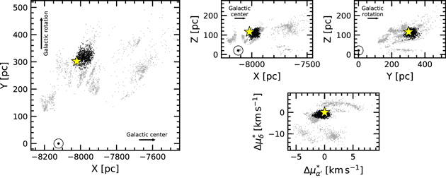
Figure 1. Galactic positions and tangential velocities of stars in the δ Lyr cluster. Points are reported cluster members from Kounkel & Covey (2019). The tangential velocities relative to Kepler 1627 (bottom right) are computed assuming that every star has the same three-dimensional spatial velocity as Kepler 1627. Our analysis considers stars (black points) in the spatial and kinematic vicinity of Kepler 1627 (yellow star). The question of whether the other candidate cluster members (gray points) are part of the cluster is outside our scope. The location of the Sun (⊙) is shown to clarify the direction along which parallax uncertainties are expected to produce erroneous clusters.
Download figure:
Standard image High-resolution image
Figure 2. Kepler's view of the δ Lyr cluster, shown in equatorial coordinates. Each black circle is a candidate cluster member selected based on its position and kinematics (Figure 1). Of the 1201 candidate cluster members, 58 have at least one quarter of Kepler data. TESS has also observed most of the cluster, for one to two lunar months to date.
Download figure:
Standard image High-resolution image2.2. The Cluster's Age
2.2.1. Color−Absolute Magnitude Diagram
We measured the isochrone age using an empirical approach. The upper-left panel of Figure 3 shows the color−absolute magnitude diagram (CAMD) of candidate δ Lyr cluster members, IC 2602 (≈38 Myr), the Pleiades (≈115 Myr), and the field. The stars from the Pleiades and IC 2602 were adopted from Cantat-Gaudin et al. (2018), and the field stars are from the Gaia EDR3 Catalog of Nearby Stars (Gaia Collaboration et al. 2021b). We also compared against μ Tau (62 ± 7 Myr; Gagné et al. 2020) and the Upper Centaurus−Lupus (UCL) component of the Sco OB2 association (≈16 Myr; Pecaut & Mamajek 2016). We adopted the UCL members from Damiani et al. (2019). For visual clarity, the latter two clusters are not shown in Figure 3. We cleaned the membership lists following the data filtering criteria from Gaia Collaboration et al. (2018a, Appendix B), except that we weakened the parallax precision requirement to ϖ/σϖ > 5. This also involved cuts on the photometric signal-to-noise ratio, the number of visibility periods used, the astrometric χ2 of the single-source solution, and the GBP − GRP color excess factor. These filters were designed to include genuine binaries while omitting instrumental artifacts.

Figure 3. The δ Lyr cluster is  Myr old. Top: color−absolute magnitude diagram of candidate δ Lyr cluster members, in addition to stars in IC 2602 (≈38 Myr), the Pleiades (≈115 Myr), and the Gaia EDR3 Catalog of Nearby Stars (gray background). The zoomed right panel highlights the pre-main sequence. The δ Lyr cluster and IC 2602 are approximately the same isochronal age. Bottom: TESS and Kepler stellar rotation period vs. dereddened Gaia color, with the Pleiades and Praesepe (650 Myr) shown for reference (Rebull et al. 2016; Douglas et al. 2017). Most candidate δ Lyr cluster members are gyrochronally younger than the Pleiades; outliers are probably field interlopers.
Download figure:
Standard image High-resolution imageTo correct for extinction, we queried the three-dimensional maps of Capitanio et al. (2017) and Lallement et al. (2018), 18 and applied the extinction coefficients kX ≡ AX /A0 computed by Gaia Collaboration et al. (2018a) assuming that A0 = 3.1E(B − V). For UCL, IC 2602, the Pleiades, and the δ Lyr cluster, this procedure yielded a respective mean and standard deviation for the reddening of E(B − V) = {0.084 ± 0.041, 0.020 ± 0.003, 0.045 ± 0.008, 0.032 ± 0.006}. These values are within a factor of two of previously reported values in the literature (Pecaut & Mamajek 2016; Gaia Collaboration et al. 2018a; Kounkel & Covey 2019; Bossini et al. 2019), and are all small enough that the choice of whether to use them versus other extinction estimates does not affect our primary conclusions.
Figure 3 shows that the δ Lyr cluster and IC 2602 overlap, and therefore they are approximately the same age. The pre-main-sequence M dwarfs of a fixed color in the δ Lyr cluster are more luminous than those of the Pleiades, and were also seen to be less luminous than those in UCL. To turn this heuristic interpolation into a quantitative age measurement, we used the empirical method developed by Gagné et al. (2020). In brief, we fitted the pre-main-sequence loci of a set of reference clusters, and the locus of the target δ Lyr cluster was then modeled as a piecewise linear combination of these reference clusters. For our reference clusters, we used UCL, IC 2602, and the Pleiades. We removed binaries by requiring RUWE < 1.3 and radial_velocity_error be below the 80th percentile of each cluster's distribution, and we excluded stars that were obvious photometric binaries in the CAMD. 19 We then passed a moving box average and standard deviation across the CAMD in 0.10 mag bins, fitted a univariate spline to the binned values, and assembled a piecewise grid of isochrones spanning the ages between UCL and the Pleiades using Equation (6) from Gagné et al. (2020). To derive a probability distribution function for the age of the δ Lyr cluster, we then assumed a Gaussian likelihood that treated the interpolated isochrones as the "model" and the δ Lyr cluster's isochrone as the "data" (Equation (7) from Gagné et al. 2020). The cluster's age and its statistical uncertainty are then quoted as the mean and standard deviation of this age posterior.
The ages returned by this procedure depend on the ages assumed for each reference cluster. We adopted a 115 Myr age for the Pleiades (Dahm 2015), and a 16 Myr age for UCL (Pecaut & Mamajek 2016). The age of IC 2602 however is the most important ingredient, since it receives the most weight in the interpolation. Plausible ages for IC 2602 span 30 Myr to 46 Myr, with older ages being preferred by the lithium-depletion-boundary (LDB) measurements (Dobbie et al. 2010; Randich et al. 2018) and younger ages by the main-sequence turnoff (Stauffer et al. 1997; David & Hillenbrand 2015; Bossini et al. 2019). If we were to adopt the 30 Myr age for IC 2602, then the δ Lyr cluster would be  Myr old. For the converse extreme of 46 Myr, the δ Lyr cluster would be
  Myr old. We adopt an intermediate 38 Myr age for IC 2602, which yields an age for the δ Lyr cluster of
  Myr.
20
Follow-up studies of the LDB or main-sequence turnoff in the δ Lyr cluster could help determine a more precise and accurate age for the cluster, and are left for future work.
Myr.
20
Follow-up studies of the LDB or main-sequence turnoff in the δ Lyr cluster could help determine a more precise and accurate age for the cluster, and are left for future work.
2.2.2. Stellar Rotation Periods
Of the 3071 candidate δ Lyr cluster members reported by Kounkel & Covey (2019), 924 stars were amenable to rotation period measurements (G < 17 and  ) using the TESS full frame image data. As a matter of scope, we restricted our attention to the 391 stars discussed in Section 2.1 in the spatial and kinematic proximity of Kepler 1627. We extracted light curves from the TESS images using the nearest pixel to each star, and regressed them against systematics with the causal pixel model implemented in the unpopular package (Hattori et al. 2021). We then measured candidate rotation periods using a Lomb–Scargle periodogram (Lomb 1976; Scargle 1982; Astropy Collaboration et al. 2018). To enable cuts on crowding, we queried the Gaia source catalog for stars within a 21
 0 radius of the target star (a radius of 1 TESS pixel). Within this radius, we recorded the number of stars with greater brightness than the target star, and with brightness within 1.25 TESS magnitudes of the target star.
We then cleaned the candidate TESS rotation period measurements through a combination of automated and manual steps. First, to validate the TESS rotation periods, we compared against 28 stars from McQuillan et al. (2014) that were also observed by Kepler. Of the 23 stars with Kepler periods below 10 days, 21 of the TESS periods agreed with the Kepler rotation periods; the other 2 were measured at the double-period harmonic. Of the remaining five stars with Kepler rotation periods above 10 days, none were correctly recovered by TESS, and three were near the half-period harmonic. We were therefore wary of any TESS rotation periods exceeding 10 days, and used the Kepler rotation periods whenever possible. For the remaining stars with only TESS data, we focused only on the stars for which no companions were known with a brightness exceeding one-tenth of the target star in a 210 radius. There were 192 stars that met these crowding requirements and that had TESS data available. For plotting purposes we then imposed a selection based on the strength of the signal itself: we required the Lomb−Scargle power to exceed 0.2, and the period to be below 15 days.
The lower panel of Figure 3 shows the resulting 145 stars. The majority of these stars fall below the "slow sequence" of the Pleiades, consistent with a gyrochronal age for the δ Lyr cluster below 100 Myr. In fact, the rotation−color distributions of other 30 Myr to 50 Myr clusters (e.g., IC 2602 and IC 2391) are indistinguishable (Douglas et al. 2021). Approximately 10 of the δ Lyr cluster stars appear as outliers above the "slow sequence." Assuming that they are all false positives (i.e., field interlopers), our rotation period detection fraction would be 135/192 ≈ 70%. Although some of these outlier stars might be unresolved F + K binaries that are in the cluster (Stauffer et al. 2016), assuming that they are field contaminants provides a more secure lower bound of the rotation period detection fraction. A final possible confounding factor—binarity—is known to affect the "fast sequence" of stars beneath the slow sequence (Meibom et al. 2007; Gillen et al. 2020; Bouma et al. 2021). We do not expect it to change the central conclusion regarding the cluster's age.
3. The Stars
3.1. Kepler 1627A
3.1.1. Age
Based on the spatial and kinematic association of Kepler 1627 with the δ Lyr cluster and the assumption that the planet formed shortly after the star, it seems likely that Kepler 1627 is the same age as the cluster. There are two consistency checks on whether this is true: rotation and lithium. Based on the Kepler light curve, the rotation period is 2.642 ± 0.042 days, where the quoted uncertainty is based on the scatter in rotation periods measured from each individual Kepler quarter. This is consistent with comparable cluster members (Figure 3).
To infer the amount of Li i from the 6708 Å doublet (e.g., Soderblom et al. 2014), we acquired an iodine-free spectrum from Keck/HIRES on the night of 2021 March 26 using the standard setup and reduction techniques of the California Planet Survey (Howard et al. 2010). Following the equivalent width measurement procedure described by Bouma et al. (2021), we find  mÅ. This value does not correct for the Fe i blend at 6707.44 Å. Nonetheless, given the stellar effective temperature (Table 1), this measurement is in agreement with expectations for a ≈40 Myr star (e.g., as measured in IC 2602 by Randich et al. 2018). It is also larger than any lithium equivalent widths measured by Berger et al. (2018) in their analysis of 1301 Kepler star spectra.
Table 1. Literature and Measured Properties for Kepler 1627
| Primary Star | |||
|---|---|---|---|
| TIC 120105470 | |||
| GAIADR2 a 2103737241426734336 | |||
| Parameter | Description | Value | Source |
| αJ2015.5 | R.A. (hh:mm:ss) | 18:56:13.6 | 1 |
| δJ2015.5 | decl. (dd:mm:ss) | +41:34:36.22 | 1 |
| V | Johnson V mag | 13.11 ± 0.08 | 2 |
| G | Gaia G mag | 13.02 ± 0.02 | 1 |
| GBP | Gaia BP mag | 13.43 ± 0.02 | 1 |
| GRP | Gaia RP mag | 12.44 ± 0.02 | 1 |
| T | TESS T mag | 12.53 ± 0.02 | 2 |
| J | 2MASS J mag | 11.69 ± 0.02 | 3 |
| H | 2MASS H mag | 11.30 ± 0.02 | 3 |
| KS | 2MASS KS mag | 11.19 ± 0.02 | 3 |
| π | Gaia EDR3 parallax (mas) | 3.009 ± 0.032 | 1 |
| d | Distance (pc) | 329.5 ± 3.5 | 1, 4 |
| μα | Gaia EDR3 proper motion in R.A. (mas yr−1) | 1.716 ± 0.034 | 1 |
| μδ | Gaia EDR3 proper motion in decl. (mas yr−1) | −1.315 ± 0.034 | 1 |
| RUWE | Gaia EDR3 renormalized unit weight error | 2.899 | 1 |
| RV | Systemic radial velocity (km s−1) | −16.7 ± 1.0 | 5 |
| Spec. Type | Spectral type | G8V | 5 |

| Rotational velocity b (km s−1) | 18.9 ± 1.0 | 5 |
| Li EW | 6708 Å equivalent width (mÅ) |

| 5 |
| Teff | Effective temperature (K) | 5505 ± 60 | 6 |

| Surface gravity (cgs) | 4.53 ± 0.05 | 6 |
| R⋆ | Stellar radius (R⊙) | 0.881 ± 0.018 | 6 |
| M⋆ | Stellar mass (M⊙) | 0.953 ± 0.019 | 6 |
| AV | Interstellar reddening (mag) | 0.2 ± 0.1 | 6 |
| [Fe/H] | Metallicity | 0.1 ± 0.1 | 6 |
| Prot | Rotation period (days) | 2.642 ± 0.042 | 7 |
| Age | Adopted stellar age (Myr) |

| 8 |
| Δm832 | Mag difference ('Alopeke 832 nm) | 3.14 ± 0.15 | 9 |
| θB | Position angle (deg) | 92 ± 1 | 9 |
| ρB | Apparent separation of primary and secondary (arcseconds) | 0.164 ± 0.002 | 9 |
| ρB | Apparent separation of primary and secondary (au) | 53 ± 4 | 1,4,9 |

| Mag difference (NIRC2  ) ) | 2.37 ± 0.02 | 10 |
| θB | Position angle (deg) | 95.9 ± 0.5 | 10 |
| ρB | Apparent separation of primary and secondary (arcseconds) | 0.1739 ± 0.0010 | 10 |
Notes. Provenances are: (1) Gaia Collaboration (2021a), (2) Stassun et al. (2019), (3) Skrutskie et al. (2006), (4) Lindegren et al. (2021), (5) HIRES spectra and Yee et al. (2017), (6) Cluster isochrone (MIST adopted; PARSEC compared for quoted uncertainty), (7) Kepler light curve, (8) Pre-main-sequence CAMD interpolation (Section 2.2.1), (9) 'Alopeke imaging, 2021 June 24 (Scott et al. 2021), and (10) NIRC2 imaging 2015 July 22, using the Yelda et al. (2010) optical distortion solution to convert pixel−space relative positions to on-sky relative astrometry. The "discrepancy" between the two imaging epochs likely indicates orbital motion.
a The GAIADR2 and GAIAEDR3 identifiers for Kepler 1627A are identical. The secondary is not resolved in the Gaia point-source catalog. b Given only and 2π
R⋆/Prot,
and 2π
R⋆/Prot,  .
.Download table as: ASCIITypeset image
3.1.2. Stellar Properties
The adopted stellar parameters are listed in Table 1. The stellar mass, radius, and effective temperature are found by interpolating against a 38 Myr MIST isochrone (Choi et al. 2016). The statistical uncertainties are propagated from the absolute magnitude (mostly originating from the parallax uncertainty) and the color; the systematic uncertainties are taken to be the difference between the PARSEC (Bressan et al. 2012) and MIST isochrones. Reported uncertainties are a quadrature sum of the statistical and systematic components. As a consistency check, we analyzed the aforementioned Keck/HIRES spectrum from the night of 2021 March 26 using a combination of SpecMatch-Emp for the stellar properties (Yee et al. 2017) and SpecMatch-Synth for  (Petigura et al. 2017
). This procedure yielded Teff = 5498 ± 100 K,
(Petigura et al. 2017
). This procedure yielded Teff = 5498 ± 100 K,  , and [Fe/H] = 0.15 ± 0.10 from SpecMatch-Emp, and
  from SpecMatch-Synth. These values are within the 1σ uncertainties of our adopted values from the isochrone interpolation.
3.2. Kepler 1627B
We first noted the presence of a close neighbor in the Kepler 1627 system on 2015 July 22 when we acquired adaptive optics imaging using the NIRC2 imager on Keck II. We used the narrow camera (Field of view = 10.2'') to obtain eight images in the  filter (λ = 2.12 μm) with a total exposure time of 160 s. We analyzed these data following Kraus et al. (2016), which entailed using point-spread function (PSF) fitting to measure the separation, position angle, and contrast of the candidate companion. The best-fitting empirical PSF template was identified from among the near-contemporaneous observations of single stars in the same filter. The mean values inferred from the eight images are reported in Table 1. To estimate the detection limits, we analyzed the residuals after subtracting the empirical PSF template. Within each residual image, the flux was measured through 40 mas apertures centered on every pixel, and then the noise as a function of radius was estimated from the rms within concentric rings. Finally, the detection limits were estimated from the strehl-weighted sum of the detection significances in the image stack, and we adopted the 6σ threshold as the detection limit for ruling out additional companions.
We also observed Kepler 1627 on Gemini North using the 'Alopeke speckle imager on 2021 June 24. 'Alopeke is a dual-channel speckle interferometer that uses narrowband filters centered at 0.83 μm and 0.56 μm. We acquired three sets of 1000 × 60 ms exposures during good seeing (045), and used the autocorrelation function of these images to reconstruct a single image and 5σ detection limits (see Howell et al. 2011). This procedure yielded a detection of the companion in the 0.83 μm notch filter, but not the 0.56 μm filter. The measured projected separation and magnitude difference are given in Table 1.
Figure 4 summarizes the results of the high-resolution imaging. The Gaia EDR3 parallax for the primary implies a projected separation of 53 ± 4 au, assuming the companion is bound. Although the companion is unresolved in the Gaia source catalog (there are no comoving, codistant candidate companions brighter than G < 20.5 mag within ρ < 120''), its existence was also suggested by the primary star's large RUWE relative to other members of the δ Lyr cluster (RUWE ≈ 2.9; roughly the 98th percentile of the cluster's distribution). Based on the apparent separation, the binary orbital period is of order hundreds of years. The large RUWE is therefore more likely to be caused by a PSF mismatch skewing the Gaia centroiding during successive scans, rather than true astrometric motion. Regardless, given the low geometric probability that a companion imaged at ρ ≈ 016 is a chance line-of-sight companion, we proceed under the assumption that the companion is bound, and that Kepler 1627 is a binary. Given the distance and age, the models of Baraffe et al. (2015) imply a companion mass MB ≈ 0.30 M⊙ and a companion temperature Teff,B ≈ 3408 K. The corresponding spectral type is roughly M3V (Pecaut & Mamajek 2013). These models combined with the NIRC2 contrast limits imply physical limits on tertiary companions of Mter < 50 MJup at ρ = 50 au, Mter < 20 MJup at ρ = 100 au, and Mter < 10 MJup at ρ = 330 au.
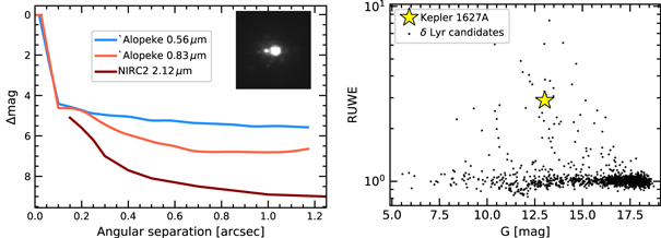
Figure 4. Kepler 1627 is a binary. Left: High-resolution imaging from Gemini North/'Alopeke and Keck/NIRC2 shows an ≈M3V companion at ρ ≈ 016, which corresponds to a projected separation of 53 ± 4 au. The inset shows a cutout of the stacked NIRC2 image (North is up, East is left, and the scale is set by the separation of the binary). The lines show 5σ contrast limits for the 'Alopeke filters, and 6σ contrast limits for NIRC2 outside of 015. Right: Gaia EDR3 renormalized unit weight error (RUWE) point estimates for candidate δ Lyr cluster members. Since other members of the cluster with similar brightnesses have comparable degrees of photometric variability, the high RUWE independently suggests that Kepler 1627 is a binary.
Download figure:
Standard image High-resolution image4. The Planet
4.1. Kepler Light Curve
The Kepler space telescope observed Kepler 1627 at a 30 minute cadence from 2009 May 2 until 2013 April 8. Data gaps during quarters 4, 9, and 13 led to an average duty cycle over the 3.9 yr interval of 67%. Kepler 1627 was also observed at 1 minute cadence from 2012 October 5 until 2013 January 11. Figure 5 shows a portion of the 30 minute cadence PDCSAP light curve. Nonastrophysical variability has been removed using the methods discussed by Smith et al. (2017); the default optimal aperture was assumed (Smith et al. 2016). Cadences with nonzero quality flags (9% of the data) have been omitted. The resulting photometry is dominated by a quasi-periodic starspot signal with a peak-to-peak amplitude that varies between 2% and 8%. Given that the secondary companion's brightness in the Kepler band is ≈1.5% that of the primary, source confusion for the rotation signal is not expected to be an issue. Previous analyses have identified and characterized the smaller transit signal (Tenenbaum et al. 2012; Thompson et al. 2018), validated its planetary nature (Morton et al. 2016), and even searched the system for transit timing variations (Holczer et al. 2016). Nonetheless, since the cluster membership provides us with more precise stellar parameters than those previously available, we opted to reanalyze the light curve.
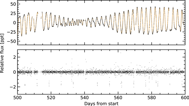
Figure 5.
The light curve of Kepler 1627. The Kepler data span 1437 days (3.9 yr), sampled at 30 minute cadence; a 100 day segment is shown. The top panel shows the PDCSAP median-subtracted flux in units of parts-per-thousand (×10−3). The dominant signal is induced by starspots. The stellar variability model (orange line) is subtracted below, revealing the transits of Kepler 1627Ab. The Figure Set spans the entire 3.9 yr of observations. The complete figure set (11 images) is available in the online journal. (The complete figure set (15 images) is available.)
Download figure:
Standard image High-resolution image4.1.1. Transit and Stellar Variability Model
We fitted the Kepler long cadence time series with a model that simultaneously included the planetary transit and the stellar variability. The stellar variability was modeled with the RotationTerm Gaussian Process kernel in exoplanet (Foreman-Mackey et al. 2021). This kernel assumes that the variability is generated by a mixture of two damped simple harmonic oscillators with characteristic frequencies set by 1/Prot and its first harmonic. We additionally included a jitter term to inflate the flux uncertainties in a manner that accounted for otherwise unmodeled excess white noise, and let the eccentricity float. For the limb darkening, we assumed a quadratic law, and sampled using the uninformative prior suggested by Kipping (2013).
Our model therefore included 10 free parameters for the transit ( ), 2 free parameters for the light-curve normalization and a white-noise jitter ({〈f〉, σf
}), and 5 hyperparameters for the GP ({σrot, Prot, Q0, dQ, f}). We also considered including an additive SHOTerm kernel to account for stochastic noise, but found that this did not affect the results, and so opted for the simpler GP kernel. We fitted the models using PyMC3 (Salvatier et al. 2016; Theano Development Team 2016), and accounted for the finite integration time of each exposure in the numerical integration when evaluating the model light curve (see Kipping 2010). We assumed a Gaussian likelihood, and after initializing each model with the parameters of the maximum a posteriori model, we sampled using PyMC3's gradient-based No-U-Turn Sampler (Hoffman & Gelman 2014) in the bases indicated in Table 2. We used
), 2 free parameters for the light-curve normalization and a white-noise jitter ({〈f〉, σf
}), and 5 hyperparameters for the GP ({σrot, Prot, Q0, dQ, f}). We also considered including an additive SHOTerm kernel to account for stochastic noise, but found that this did not affect the results, and so opted for the simpler GP kernel. We fitted the models using PyMC3 (Salvatier et al. 2016; Theano Development Team 2016), and accounted for the finite integration time of each exposure in the numerical integration when evaluating the model light curve (see Kipping 2010). We assumed a Gaussian likelihood, and after initializing each model with the parameters of the maximum a posteriori model, we sampled using PyMC3's gradient-based No-U-Turn Sampler (Hoffman & Gelman 2014) in the bases indicated in Table 2. We used  as our convergence diagnostic (Gelman & Rubin 1992).
Table 2. Priors and Posteriors for Model Fitted to the Long Cadence Kepler 1627Ab Light Curve
| Param. | Unit | Prior | Median | Mean | Std. Dev. | 3% | 97% | ESS |

|
|---|---|---|---|---|---|---|---|---|---|
| Sampled | |||||||||
| P | days |
| 7.2028038 | 7.2028038 | 0.0000073 | 7.2027895 | 7.2028168 | 7464 | 3.9e-04 |
 1
1
| days |
| 120.7904317 | 120.7904254 | 0.0009570 | 120.7886377 | 120.7921911 | 3880 | 2.0e-03 |

| ⋯ |
| −6.3430 | −6.3434 | 0.0354 | −6.4094 | −6.2767 | 6457 | 3.0e-04 |
| b 2 | ⋯ |

| 0.4669 | 0.4442 | 0.2025 | 0.0662 | 0.8133 | 1154 | 1.6e-03 |
| u1 | ⋯ | Kipping (2013) | 0.271 | 0.294 | 0.190 | 0.000 | 0.628 | 3604 | 1.5e-03 |
| u2 | ⋯ | Kipping (2013) | 0.414 | 0.377 | 0.326 | −0.240 | 0.902 | 3209 | 1.4e-03 |
| R⋆ | R⊙ |

| 0.881 | 0.881 | 0.018 | 0.847 | 0.915 | 8977 | 3.1e-04 |

| cgs |

| 4.532 | 4.533 | 0.051 | 4.435 | 4.627 | 6844 | 1.6e-03 |
| 〈f〉 | ⋯ |

| −0.0003 | −0.0003 | 0.0001 | −0.0005 | −0.0000 | 8328 | 1.1e-03 |
| e 3 | ⋯ | Van Eylen et al. (2019) | 0.154 | 0.186 | 0.152 | 0.000 | 0.459 | 1867 | 2.0e-03 |
| ω | rad |

| 0.055 | 0.029 | 1.845 | −3.139 | 2.850 | 3557 | 8.6e-05 |

| ⋯ |
| −8.035 | −8.035 | 0.008 | −8.049 | −8.021 | 9590 | 3.9e-04 |
| σrot | days−1 | InvGamma(1.000; 5.000) | 0.070 | 0.070 | 0.001 | 0.068 | 0.072 | 9419 | 1.4e-03 |

|

|

| 0.978 | 0.978 | 0.001 | 0.975 | 0.980 | 8320 | 2.2e-04 |
| log Q0 | ⋯ |

| −0.327 | −0.326 | 0.043 | −0.407 | −0.246 | 9659 | 2.7e-04 |
| log d Q | ⋯ |

| 7.697 | 7.698 | 0.103 | 7.511 | 7.899 | 5824 | 3.7e-04 |
| f | ⋯ |

| 0.01006 | 0.01009 | 0.00009 | 0.01000 | 0.01025 | 4645 | 4.0e-04 |
| Derived | |||||||||
| δ | ⋯ | ⋯ | 0.001759 | 0.001759 | 0.000062 | 0.001641 | 0.001875 | 6457 | 3.0e-04 |
| Rp/R⋆ | ⋯ | ⋯ | 0.039 | 0.039 | 0.001 | 0.037 | 0.042 | 1811 | 1.1e-03 |
| ρ⋆ | g cm−3 | ⋯ | 1.990 | 2.004 | 0.240 | 1.570 | 2.461 | 6905 | 2.1e-03 |
 4
4
| RJup | ⋯ | 0.337 | 0.338 | 0.014 | 0.314 | 0.367 | 2311 | 1.0e-03 |
 4
4
| REarth | ⋯ | 3.777 | 3.789 | 0.157 | 3.52 | 4.114 | 2311 | 1.0e-03 |
| a/R⋆ | ⋯ | ⋯ | 17.606 | 17.619 | 0.702 | 16.277 | 18.906 | 6905 | 2.1e-03 |

| ⋯ | ⋯ | 0.027 | 0.025 | 0.010 | 0.004 | 0.040 | 1312 | 1.2e-03 |
| T14 | hr | ⋯ | 2.841 | 2.843 | 0.060 | 2.734 | 2.958 | 3199 | 3.6e-04 |
| T13 | hr | ⋯ | 2.555 | 2.539 | 0.094 | 2.360 | 2.692 | 1960 | 1.4e-03 |
Note. ESS refers to the number of effective samples.  is the Gelman−Rubin convergence diagnostic. Logarithms in this table are base-e.
  denotes a uniform distribution, and
  a normal distribution.
 is formally correct, for this model we assumed a nongrazing transit to enable sampling in
  .
3
The eccentricity vectors are sampled in the
.
3
The eccentricity vectors are sampled in the  plane.
4
The true planet size is a factor of
plane.
4
The true planet size is a factor of  larger than that from the fit because of dilution from Kepler 1627B, where F1 is the flux from the primary, and F2 is that from the secondary; the mean and standard deviation of Rp = 3.817 ± 0.158 R⊕ quoted in the text includes this correction, assuming (F1+F2)/F1 ≈ 1.015.
Download table as: ASCIITypeset image
Figure 5 shows the resulting best-fit model in orange and Figure 6 shows the resulting best-fit model in purple. The model parameters and their uncertainties, given in Table 2, are broadly consistent with a Neptune-sized planet (3.82 ± 0.16 R⊕) on a close-in circular 21 orbit around a G8V host star (0.88 ± 0.02 R⊙). This best-fit planet size is consistent with those previously reported by Morton et al. (2016) and Berger et al. (2018), and corrects for the small amount of flux dilution from Kepler 1627B.
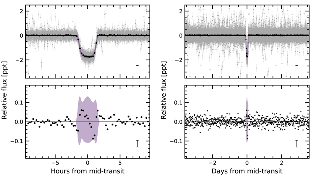
Figure 6. Phase-folded transit of Kepler 1627Ab with stellar variability removed. Windows over 20 hr (left) and the entire orbit (right) are shown, and the residual after subtracting the transit is in the bottom row. The 2σ model uncertainties and the best-fit model are the light purple band and the dark purple line. Gray points are individual flux measurements; black points bin these into 15 minute intervals and have a representative 1σ error bar in the lower right of each panel. The asymmetric residual during transit is larger than the out-of-transit scatter.
Download figure:
Standard image High-resolution image4.1.2. Transit Asymmetry
The transit fit, however, is not perfect: Figure 6 shows an asymmetric residual in the data relative to the model: the measured flux is high during the first half of transit, and low in the second half. The semiamplitude of this deviation is ≈50 ppm, which represents a ≈3% distortion of the transit depth (δ = 1759 ± 62 ppm). Note that although this asymmetry is within the 2σ model uncertainties, the model has a jitter term that grows to account for excess white noise in the flux. The significance of the asymmetry is therefore best assessed in comparison against the intrinsic out-of-transit scatter in the data (≈16 ppm), not the model uncertainties. The right panel of Figure 6 demonstrates that the scatter during transit is higher than during all other phases of the planet's orbit.
To determine whether the asymmetry could be a systematic caused by our stellar variability model, we explored an alternative approach in which we isolated each transit window, locally fitted out polynomial trends, and then binned all of the observed transits; the asymmetry was still present at a comparable amplitude. Appendix B describes a more detailed analysis, which finds that the asymmetry also seems to be robust to different methods of data binning in time and by local light-curve slope. Possible astrophysical explanations are discussed in Section 5.
4.1.3. Transit Timing and the Local Slope
The previous analysis by Holczer et al. (2016) did not find any significant long-term transit timing or duration variations (TTVs or TDVs) for Kepler 1627. Quantitatively, the mean and standard deviation of the TTVs and TDVs they measured were − and −
and − . In an earlier analysis, however, Holczer et al. (2015) studied correlations between TTVs and local light-curve slopes, and for Kepler 1627 found a weak correlation of
  between the two quantities. Given the possible connection between such correlations and the unresolved starspot crossings that we expect to be present in the Kepler 1627 light curve (Mazeh et al. 2015), we opted to reexamine the individual transit times.
We therefore isolated each of the 144 observed transits to within ±4.5 hr of each transit, and fitted each window with both (1) a local second- or fourth-order polynomial baseline plus the transit, and (2) a local linear trend plus the transit. We let the midtime of each transit float, and then calculated the residual between the measured midtime and that of a periodic orbit. This residual, the transit timing variation, is plotted in Figure 7 against the local linear slope assuming the fourth-order polynomial baseline. The slope of  is similar to that found by Holczer et al. (2015). The best-fit line yields χ2 = 306.1, with n = 140 data points. An alternative model of just a flat line yields χ2 = 315.6. The difference in the Bayesian information criterion between the two models is BICflat − BICline = 4.5, which corresponds to a Bayes factor of ≈9.4. According to the usual Kass & Raftery (1995) criteria, this is "positive" evidence for the model with a finite slope. We view it as suggestive at best, particularly given the poor reduced χ2.

Figure 7. Weak evidence for a prograde orbit of Kepler 1627Ab. The time of each Kepler transit was measured, along with the local slope of the light curve. The two quantities might be anticorrelated (≈2σ), which could be caused by starspot crossings during the first (second) half of transit inducing a positive (negative) TTV, provided that the orbit is prograde (Mazeh et al. 2015). The units along the abscissa can be understood by considering that the stellar flux changes by ∼60 ppt per half rotation period (∼1.3 days).
Download figure:
Standard image High-resolution imageA separate concern we had in this analysis was whether our transit fitting procedure might induce spurious correlations between the slope and transit time. In particular, assuming the second-order polynomial baseline yielded a larger anticorrelation between the TTVs and local slopes, of  . We therefore performed an injection-recovery procedure in which we injected transits at different phases in the Kepler 1627 light curve and repeated the TTV analysis. This was done at ≈50 phases, each separated by 0.02 Porb while omitting the phases in transit. For the second-order polynomial baseline, this procedure yielded a similar anticorrelation in the injected transits as that present in the real transit; assuming this baseline would therefore bias the result. However, for the fourth-order baseline, the correlation present in the data was stronger than in all but one of the injected transits. Possible interpretations are discussed below. Given the lack of statistical significance, this analysis should be interpreted as suggestive at best.
4.2. Planet Confirmation
If the Kepler 1627Ab transit signal is created by a genuine planet, then to our knowledge it would be the youngest planet yet found by the prime Kepler mission. 22 Could the transit be produced by anything other than a planet orbiting this near-solar analog? Morton et al. (2016) validated the planet based on the transit shape, arguing that the most probable false-positive scenario was that of a background eclipsing binary, which had a model-dependent probability of ≈10−5. However, this calculation was performed without knowledge of the low-mass stellar companion (MB ≈ 0.30 M⊙). Validated planets have also previously been refuted (e.g., Shporer et al. 2017). We therefore reassessed false-positive scenarios in some detail.
As an initial plausibility check, Kepler 1627B contributes 1%–2% of the total flux observed in the Kepler aperture. For the sake of argument, assume the former value. The observed transit has a depth of ≈0.18%. An ≈18% deep eclipse of Kepler 1627B would therefore be needed to produce a signal with the appropriate depth. The shape of the transit signal, however, requires the impact parameter to be below 0.77 (2σ); the tertiary transiting the secondary would therefore need to be nongrazing with R3/R2 ≈ 0.4. This yields a contradiction: this scenario requires an ingress and egress phase that each span ≈40% of the transit duration (≈68 min). The actual measured ingress and egress duration is ≈ , a factor of four times too short. The combination of Kepler 1627B's brightness, the transit depth, and the ingress duration therefore disfavor the scenario that Kepler 1627B might host the transit signal.
Beyond this simple test, a line of evidence that effectively confirms the planetary interpretation is that the stellar density implied by the transit duration and orbital period is inconsistent with an eclipsing body around the M-dwarf companion. We find ρ⋆ = 2.00 ± 0.24 g cm−3, while the theoretically expected density for Kepler 1627B given its nominal age of 38 Myr and mass of 0.30 M⊙ is ≈4.6 g cm−3 (Baraffe et al. 2015). The transit duration is therefore too long to be explained by a star eclipsing the M-dwarf secondary at 10σ. Alternatively, assuming a younger age (32 Myr) and a larger companion mass (0.35 M⊙), the companion's density could be as low as ≈3.5 g cm−3. This is still in tension with the fitted stellar density. While the planet might hypothetically still orbit a hidden close and bright companion, this possibility is implausible given (1) the lack of secondary lines in the HIRES spectra, (2) the lack of secondary rotation signals in the Kepler photometry, and (3) the proximity of Kepler 1627 to the δ Lyr cluster locus on the Gaia CAMD (Figure 3).
The correlation noted in Section 4.1.3 between the TTVs and the local light-curve slope might be an additional line of evidence in support of the planetary interpretation. Unless it is a statistical fluke (a ≈5% possibility), then the most likely cause of the correlation is unresolved starspot crossings (Mazeh et al. 2015). These would only be possible if the planet transits the primary star, which excludes a background eclipsing binary scenario. The correlation would also suggest that the planet's orbit is prograde. The latter point assumes that the dominant photometric variability is induced by dark spots, and not bright faculae. Given the observed transition of Sun-like stellar variability from spot to faculae-dominated regimes between young and old ages, we expect this latter assumption to be reasonably secure (Shapiro et al. 2016; Montet et al. 2017; Reinhold & Hekker 2020).
A third supporting line of evidence for the planetary interpretation also exists. We observed a transit of Kepler 1627Ab on the night of 2021 August 7 spectroscopically with HIRES on the Keck I telescope and photometrically in griz bands with MuSCAT3 at Haleakalā Observatory. Details of the observation sequence are discussed in Appendix C; Figure 8 shows the results. Although we did not detect the Rossiter−McLaughlin (RM) anomaly, the multiband MuSCAT3 light curves show that the transit is achromatic. Quantitatively, when we fitted the MuSCAT3 photometry with a model that lets the transit depths vary across each bandpass, we found griz depths consistent with the Kepler depth at 0.6, 0.3, 0.3, and 1.1σ, respectively. The achromatic transits strongly favor Kepler 1627A as the transit host, since Kepler 1627B is a much redder star. Conditioned on the ephemeris and transit depth from the Kepler data, the MuSCAT3 observations also suggested a transit duration  shorter than the Kepler transits. However, given both the lack of TDVs in the Kepler data and the relatively low signal-to-noise ratio of the MuSCAT3 transit, further photometric follow-up would be necessary to determine whether the transit duration is actually changing.
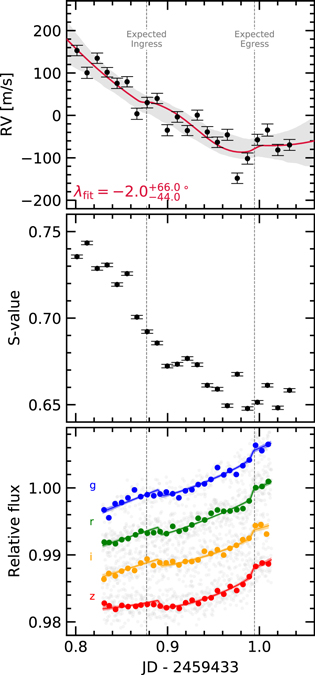
Figure 8. Keck/HIRES radial velocities and MuSCAT3 photometry from the transit of 2021 Aug 7. Top: the radial velocity jitter across the 15 minute exposures (σRV ≈ 30 m s−1) prevented us from detecting the RM effect; a model including the RM anomaly and a quadratic trend in time to fit the spot-induced ≈250 m s−1 trend is shown (see Appendix C). Shaded bands show 2σ model uncertainties. Middle: the RV variations are strongly correlated with varying emission in the Ca H and K lines. Bottom: the photometric transit depths are consistent across the griz bandpasses. The photometry is binned at 10 minute intervals.
Download figure:
Standard image High-resolution imageFor our RM analysis, the details are discussed in Appendix C. While the velocities are marginally more consistent with a prograde or polar orbit than a retrograde orbit, the spot-corrected exposure-to-exposure scatter (σRV ≈ 30 m s−1) is comparable to the expected RM anomaly assuming an aligned orbit (ΔvRM ≈ 20 m s−1). We are therefore not in a position to claim a spectroscopic detection of the RM effect, nor to quantify the stellar obliquity.
5. Discussion and Conclusions
Kepler 1627Ab provides a new extremum in the ages of the Kepler planets, and opens multiple avenues for further study. Observations of spectroscopic transits at greater signal-to-noise ratios should yield a measurement of the stellar obliquity, which would confirm or refute the prograde orbital geometry suggested by the TTV−local slope correlation. Separately, transit spectroscopy aimed at detecting atmospheric outflows could yield insight into the evolutionary state of the atmosphere (e.g., Ehrenreich et al. 2015; Spake et al. 2018; Vissapragada et al. 2020). Observations that quantify the amount of high-energy irradiation incident on the planet would complement these efforts by helping to clarify the expected outflow rate (e.g., Poppenhaeger et al. 2021). Finally, a challenging but informative quantity to measure would be the planet's mass. Measured at sufficient precision, for instance through a multiwavelength radial velocity campaign, the combination of the size, mass, and age would yield constraints on both the planet's composition and its initial entropy (Owen 2020).
More immediately, the Kepler data may yet contain additional information. For instance, one possible explanation for the transit asymmetry shown in Figure 6 is that of a dusty asymmetric outflow. Dusty outflows are theoretically expected for young mini-Neptunes, and the amplitude of the observed asymmetry is consistent with predictions (Wang & Dai 2019). A second possibility is that the planetary orbit is slightly misaligned from the stellar spin axis, and tends to transit starspot groups at favored stellar latitudes. This geometry would be necessary in order to explain how the starspot crossings could add up coherently, given that the planetary orbital period (7.203 days) and the stellar rotation period (2.642 days) are not a rational combination. Other possibilities including gravity darkening or TTVs causing the asymmetry are disfavored (see Appendix B).
Beyond the asymmetric transits, Appendix D highlights an additional abnormality in the short cadence Kepler data, in the arrival time distribution of stellar flares. We encourage its exploration by investigators more versed in the topic than ourselves.
In the context of the transiting planet population, Kepler 1627Ab is among the youngest known (Figure 9). Comparable systems with precise ages include K2-33 (Mann et al. 2016; David et al. 2016), DS Tuc (Benatti et al. 2019; Newton et al. 2019), HIP 67522 (Rizzuto et al. 2020), TOI 837 (Bouma et al. 2020), the two-planet AU Mic (Plavchan et al. 2020; Martioli et al. 2021), and the four-planet V1298 Tau (David et al. 2019). Kepler 1627Ab is one of the smaller planets in this sample (3.82 ± 0.16 R⊕), which could be linked to the selection effects imposed by spot-induced photometric variability at very young ages (e.g., Zhou et al. 2021). It seems though that smaller planets could have been detected in the Kepler 1627 system: based on the per-target detection contours, the Kepler pipeline's median completeness extended to 1.6 R⊕ at 10 day orbital periods, and 3.3 R⊕ at 100 days (Burke & Catanzarite 2021). These limits account for the spot-induced variability in the system through a correction based on the Combined Differential Photometric Precision in the light curve over the relevant transit timescales (Burke & Catanzarite 2017). The large size of Kepler 1627Ab relative to most Kepler mini-Neptunes might therefore support a picture in which the typical 5 M⊕ mini-Neptune (Wu 2019) loses a significant fraction of its primordial atmosphere over its first gigayear (Owen & Wu 2013; Ginzburg et al. 2018). It could also be consistent with a scenario in which an earlier "boil-off" of the planet's atmosphere during disk dispersal decreases the entropy of the planetary interior, leading to a rather long ∼108 year Kelvin–Helmholtz contraction timescale (Owen 2020). Confirming either of these scenarios would require a measurement of the planetary mass; otherwise, alternative explanations for its large size could include that it is just abnormally massive, or that it has an abnormally large envelope to core mass ratio.
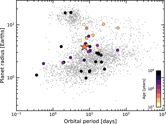
Figure 9. Radii, orbital periods, and ages of transiting exoplanets. Planets younger than a gigayear with τ/στ > 3 are emphasized, where τ is the age and στ is its uncertainty. Kepler 1627Ab is shown with a star. The large sizes of the youngest transiting planets could be explained by their primordial atmospheres not yet having evaporated; direct measurements of the atmospheric outflows or planetary masses would help to confirm this expectation. Selection effects may also be important. Parameters are from the NASA Exoplanet Archive (accessed 2021 September 15).
Download figure:
Standard image High-resolution imageUltimately, the main advance of this work is a precise measurement of the age of Kepler 1627Ab. This measurement was enabled by identifying the connection of the star to the δ Lyr cluster using Gaia kinematics, and by then using the Gaia color−absolute magnitude diagram and TESS stellar rotation periods to verify the cluster's existence. Table 3 enables similar cross-matches for both known and forthcoming exoplanet systems (e.g., Guerrero et al. 2021). Confirming these candidate associations using independent age indicators is essential because their false-positive rates are not known. A related path is to identify new kinematic associations around known exoplanet host stars using positions and tangential velocities from Gaia, and to verify these associations with stellar rotation periods and spectroscopy (e.g., Tofflemire et al. 2021). Each approach seems likely to expand the census of planets with precisely measured ages over the coming years, which will help in deciphering the early stages of exoplanet evolution.
Table 3. Young, Age-dated, and Age-dateable Stars within the Nearest Few Kiloparsecs
| Parameter | Example Value | Description |
|---|---|---|
| source_id | 1709456705329541504 | Gaia DR2 source identifier |
| ra | 247.826 | Gaia DR2 R.A. (deg) |
| dec | 79.789 | Gaia DR2 decl. (deg) |
| parallax | 35.345 | Gaia DR2 parallax (mas) |
| parallax_error | 0.028 | Gaia DR2 parallax uncertainty (mas) |
| pmra | 94.884 | Gaia DR2 proper motion  (mas yr−1) (mas yr−1) |
| pmdec | −86.971 | Gaia DR2 proper motion μδ (mas yr−1) |
| phot_g_mean_mag | 6.85 | Gaia DR2 G magnitude |
| phot_bp_mean_mag | 6.409 | Gaia DR2 GBP magnitude |
| phot_rp_mean_mag | 7.189 | Gaia DR2 GRP magnitude |
| cluster | NASAExoArchive_ps_20210506,Uma,IR_excess | Comma-separated cluster or group name |
| age | 9.48,nan,nan | Comma-separated logarithm (base-10) of reported age in years |
| mean_age | 9.48 | Mean (ignoring NaNs) of age column |
| reference_id | NASAExoArchive_ps_20210506,Ujjwal2020,CottenSong2016 | Comma-separated provenance of group membership |
| reference_bibcode | 2013PASP..125..989A,2020AJ....159..166U,2016ApJS..225...15C | ADS bibcode corresponding to reference_id |
Note. Table 3 is available as a comma delimited table in the .tar.gz package. Two Python scripts are also included to help read the variable-length string columns. This table is a concatenation of the studies listed in Table 4. One entry is shown for guidance regarding form and content. In this particular example, the star has a cold Jupiter on a 16 year orbit, HD 150706b (Boisse et al. 2012). An infrared excess has been reported (Cotten & Song 2016), and the star was identified by Ujjwal et al. (2020) as a candidate UMa moving group member (≈400 Myr; Mann et al. 2020). The star's RV activity and TESS rotation period corroborate its youth.
Download table as: ASCIITypeset image
The authors are grateful to J. Winn, J. Spake, A. Howard, and T. David for illuminating discussions and suggestions, and to R. Kerr for providing us with the Kerr et al. (2021) membership list prior to its publication. The authors are also grateful to K. Collins for helping resolve the scheduling conflict that would have otherwise prevented the MuSCAT3 observations. L.G.B. acknowledges support from a Charlotte Elizabeth Procter Fellowship from Princeton University, as well as from the TESS GI Program (NASA grant 80NSSC21K0335) and the Heising-Simons Foundation (51 Pegasi b Fellowship). Keck/NIRC2 imaging was acquired by program 2015A/N301N2L (PI: A. Kraus). In addition, this paper is based in part on observations made with the MuSCAT3 instrument, developed by the Astrobiology Center and under financial support by JSPS KAKENHI (JP18H05439) and JST PRESTO (JPMJPR1775), at Faulkes Telescope North on Maui, HI, operated by the Las Cumbres Observatory. This work is partly supported by JSPS KAKENHI Grant Nos. 22000005, JP15H02063, JP17H04574, JP18H05439, and JP18H05442, JST PRESTO grant No. JPMJPR1775, and the Astrobiology Center of National Institutes of Natural Sciences (NINS; grant No. AB031010). This paper also includes data collected by the TESS mission, which are publicly available from the Mikulski Archive for Space Telescopes (MAST). Funding for the TESS mission is provided by NASA's Science Mission directorate. We thank the TESS Architects (G. Ricker, R. Vanderspek, D. Latham, S. Seager, and J. Jenkins) and the many TESS team members for their efforts to make the mission a continued success. Finally, this research has made use of the Keck Observatory Archive (KOA), which is operated by the W. M. Keck Observatory and the NASA Exoplanet Science Institute (NExScI), under contract with the National Aeronautics and Space Administration. We also thank the Keck Observatory staff for their support of HIRES and remote observing. We recognize the importance that the summit of Maunakea has within the indigenous Hawaiian community, and are deeply grateful to have the opportunity to conduct observations from this mountain.
Software: altaipony (Ilin et al. 2021), astrobase (Bhatti et al. 2018), astropy (Astropy Collaboration et al. 2018), astroquery (Ginsburg et al. 2018), corner (Foreman-Mackey 2016), exoplanet (Foreman-Mackey et al. 2021), and its dependencies Agol et al. (2020); Kipping (2013); Luger et al. (2019); Theano Development Team (2016), PyMC3 (Salvatier et al. 2016), scipy (Jones et al. 2001), TESS-point (Burke et al. 2020), wotan (Hippke et al. 2019).
Facility: Astrometry: Gaia - (Gaia Collaboration et al. 2018b; Gaia Collaboration 2021a). Imaging: Second Generation Digitized Sky Survey. Keck:II (NIRC2; www2.keck.hawaii.edu/inst/nirc2). Gemini:North ('Alopeke; Scott et al. (2018, 2021). Spectroscopy: Keck:I (HIRES; Vogt et al. 1994). Photometry: Kepler (Borucki et al. 2010), MuSCAT3 (Narita et al. 2020), TESS (Ricker et al. 2015).
Appendix A: Young, Age-dated, and Age-dateable Star Compilation
The v0.6 CDIPS target catalog (Table 3) includes stars that are young, age-dated, and age-dateable. By "age-dateable," we mean that the stellar age should be measurable to a greater precision than that of a typical FGK field star, through either isochronal, gyrochronal, or spectroscopic techniques. As in Bouma et al. (2019), we collected stars that met these criteria from across the literature. Table 4 gives a list of the studies included, and brief summary statistics. The age measurement methodologies adopted by each study differ: in many, spatial and kinematic clustering has been performed on the Gaia data, and ensemble isochrone fitting of the resulting clusters has been performed (typically focusing on the turnoff). In other studies, however, the claim of youth is based on the location of a single star in the color−absolute magnitude diagram, or on spectroscopic information.
Table 4. Provenances of Young and Age-dateable Stars
| Reference | NGaia | NAge |

|
|---|---|---|---|
| Kounkel et al. (2020) | 987,376 | 987,376 | 775,363 |
| Cantat-Gaudin & Anders (2020) | 433,669 | 412,671 | 269,566 |
| Cantat-Gaudin et al. (2018) | 399,654 | 381,837 | 246,067 |
| Kounkel & Covey (2019) | 288,370 | 288,370 | 229,506 |
| Cantat-Gaudin et al. (2020) | 233,369 | 227,370 | 183,974 |
| Zari et al. (2018) UMS | 86,102 | 0 | 86,102 |
| Wenger et al. (2000) Y*? | 61,432 | 0 | 45,076 |
| Zari et al. (2018) PMS | 43,719 | 0 | 38,435 |
| Gaia Collaboration et al. (2018a) d > 250 pc | 35,506 | 31,182 | 18,830 |
| Castro-Ginard et al. (2020) | 33,635 | 24,834 | 31,662 |
| Kerr et al. (2021) | 30,518 | 25,324 | 27,307 |
| Wenger et al. (2000) Y *O | 28,406 | 0 | 16,205 |
| Villa Vélez et al. (2018) | 14,459 | 14,459 | 13,866 |
| Cantat-Gaudin et al. (2019) | 11,843 | 11,843 | 9246 |
| Damiani et al. (2019) PMS | 10,839 | 10,839 | 9901 |
| Oh et al. (2017) | 10,379 | 0 | 10,370 |
| Meingast et al. (2021) | 7925 | 7925 | 5878 |
| Wenger et al. (2000) pMS* | 5901 | 0 | 3006 |
| Gaia Collaboration et al. (2018a) d < 250 pc | 5378 | 817 | 3968 |
| Kounkel et al. (2018) | 5207 | 3740 | 5207 |
| Ratzenböck et al. (2020) | 4269 | 4269 | 2662 |
| Wenger et al. (2000) TT* | 4022 | 0 | 3344 |
| Damiani et al. (2019) UMS | 3598 | 3598 | 3598 |
| Rizzuto et al. (2017) | 3294 | 3294 | 2757 |
| Akeson et al. (2013) | 3107 | 868 | 3098 |
| Tian (2020) | 1989 | 1989 | 1394 |
| Goldman et al. (2018) | 1844 | 1844 | 1783 |
| Cotten & Song (2016) | 1695 | 0 | 1693 |
| Gagné et al. (2018b) | 1429 | 0 | 1389 |
| Röser & Schilbach (2020) Psc-Eri | 1387 | 1387 | 1107 |
| Röser & Schilbach (2020) Pleiades | 1245 | 1245 | 1019 |
| Wenger et al. (2000) TT? | 1198 | 0 | 853 |
| Gagné & Faherty (2018) | 914 | 0 | 913 |
| Pavlidou et al. (2021) | 913 | 913 | 504 |
| Gagné et al. (2018a) | 692 | 0 | 692 |
| Ujjwal et al. (2020) | 563 | 0 | 563 |
| Gagné et al. (2020) | 566 | 566 | 351 |
| Esplin & Luhman (2019) | 377 | 443 | 296 |
| Roccatagliata et al. (2020) | 283 | 283 | 232 |
| Meingast & Alves (2019) | 238 | 238 | 238 |
| Fürnkranz et al. (2019) Coma-Ber | 214 | 214 | 213 |
| Fürnkranz et al. (2019) Neighbor Group | 177 | 177 | 167 |
| Kraus et al. (2014) | 145 | 145 | 145 |
Note. Table 4 describes the provenances for the young and age-dateable stars in Table 3. NGaia: number of Gaia stars we parsed from the literature source. NAge: number of stars in the literature source with ages reported.  : number of Gaia stars we parsed from the literature source with either GRP < 16, or a parallax signal-to-noise ratio exceeding 5 and a distance closer than 100 pc. The latter criterion included a few hundred white dwarfs that would have otherwise been neglected. Some studies are listed multiple times if they contain multiple tables. Wenger et al. (2000) refers to the SIMBAD database.
Download table as: ASCIITypeset image
One major change in Table 3 relative to the earlier iteration from Bouma et al. (2019) is that the extent of Gaia-based analyses has now matured to the point that we can neglect pre-Gaia cluster memberships, except for a few cases with spectroscopically confirmed samples of age-dated stars. The membership lists, for instance, of Kharchenko et al. (2013) and Dias et al. (2014; MWSC and DAML) are no longer required. This is helpful for various postprocessing projects, since the field star contamination rates were typically much higher in these catalogs than in the newer Gaia-based catalogs.
The most crucial parameters of a given star for our purposes are the Gaia DR2 source_id, the cluster or group name (cluster), and the age. Given the hierarchical nature of many stellar associations, we do not attempt to resolve the cluster names to a single unique string. The Orion complex, for instance, can be divided into almost one hundred kinematic subgroups (Kounkel et al. 2018). Based on Figure 1, the δ Lyr cluster may also be part of a similar hierarchical association. Similar complexity applies to the problem of determining homogeneous ages, which we do not attempt to resolve. Instead, we simply merged the cluster names and ages reported by various authors into a comma-separated string.
This means that the age column can be null, for cases in which the original authors did not report an age, or for which a reference literature age was not readily available. Nonetheless, since we do prefer stars with known ages, we made a few additional efforts to populate this column. When available, the age provenance is from the original analysis of the cluster. In a few cases however we adopted other ages when string-based cross-matching on the cluster name was straightforward. In particular, we used the ages determined by Cantat-Gaudin et al. (2020) to assign ages to the clusters from Gaia Collaboration et al. (2018a); Cantat-Gaudin et al. (2018); Castro-Ginard et al. (2020), and Cantat-Gaudin & Anders (2020).
The catalogs we included for which ages were not immediately available were those of Cotten & Song (2016), Oh et al. (2017), Zari et al. (2018), Gagné et al. (2018a, 2018b), Gagné & Faherty (2018), and Ujjwal et al. (2020). While in principle the moving group members discussed by Gagné et al. (2018a, 2018b), Gagné & Faherty (2018), and Ujjwal et al. (2020) have easily associated ages, our SIMBAD cross-match did not retain the moving group identifiers given by those studies, which should therefore be recovered using tools such as BANYAN Σ (Gagné et al. 2018b). We also included the SIMBAD object identifiers TT*, Y *O, Y*?, TT?, and pMS*. Finally, we included every star in the NASA Exoplanet Archive planetary system (ps) table that had a Gaia identifier available (Akeson et al. 2013). If the age had finite uncertainties, we also included it, since stellar ages determined through the combination of isochrone fitting and transit-derived stellar densities typically have a higher precision than from isochrones alone.
For any of the catalogs for which Gaia DR2 identifiers were not available, we either followed the spatial (plus proper motion) cross-matching procedures described in Bouma et al. (2019), or else we pulled the Gaia DR2 source identifiers associated with the catalog from SIMBAD. We consequently opted to drop the ext_catalog_name and dist columns maintained in Bouma et al. (2019), as these were only populated for a small number of stars. The technical manipulations for the merging, cleaning, and joining were performed using pandas (McKinney 2010). The eventual cross-match (using the Gaia DR2 source_id) against the Gaia DR2 archive was performed asychronously on the Gaia archive website.
Appendix B: The Transit Asymmetry
B.1. How Robust is the Asymmetric Transit?
As a means of exploring the robustness of the transit asymmetry, Figures 10, 11, and 12 show the Kepler data binned in three ways: over Kepler quarters, Julian years, and quartiles of local slope. Over Kepler quarters (Figure 10), Quarter 6 shows the strongest asymmetry: a deviation of about 3 ppt from expectation. Quarter 7 shows an anomaly at roughly the same transit phase. Year 2 correspondingly shows the strongest anomaly out of any year in Figure 11; the asymmetry is visually apparent, however, in each of the four years.

Figure 10. Transit model residuals through time (binned by Kepler quarter). Left: phase-folded transit of Kepler 1627b, with stellar variability removed. Black points are binned to 20 minute intervals. The 2σ model uncertainties and the maximum a posteriori model are shown as the faint purple band, and the dark purple line. Right: as on the left, with the transit removed.
Download figure:
Standard image High-resolution image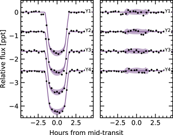
Figure 11. Transit model residuals through time (binned by year of observation). Left: phase-folded transit of Kepler 1627b, with stellar variability removed. Points and models are as in Figure 10. Right: as on the left, with the transit removed.
Download figure:
Standard image High-resolution image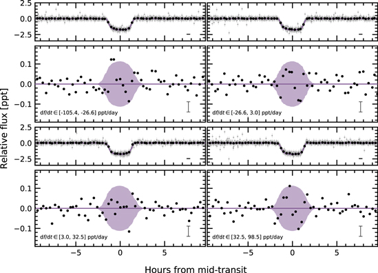
Figure 12. Transit models and residuals, binned by quartiles in the local slope of the light curve. Representative uncertainties for the black points (binned at 20 minute intervals) are shown in the lower right of each panel. A similar transit asymmetry to that shown in Figure 6 seems to be present in three of the four bins.
Download figure:
Standard image High-resolution imageTo bin by quartiles in local slope, we used our measurements of the local linear slopes in each of the observed transit windows (144 transits total). Four outlier transits were removed, leaving 140 transits. These were then divided into quartiles, so that each panel shows 35 transits binned together. The exact light-curve slope intervals are listed in the lower-left panels of Figure 12. Binned by local-slope quartiles (Figure 12), the asymmetry is visually present in three of the four quartiles: the only bin in which it does not appear is df/dt ∈ [3.0, 32.5] ppt day−1.
Within the theory presented by Mazeh et al. (2015), unresolved starspot crossings cause the weak correlation between TTVs and the local light-curve slope (Figure 7). In this model, we would expect the light curves with the most negative local slopes to have the largest positive TTVs, due to spot-crossing events during the latter half of transit. The upper-left panel of Figure 12 agrees with this expectation. However, we would also expect the sign of the effect to reverse when considering the most positive local slopes (most negative TTVs). The lower-right panel of Figure 12 contradicts this expectation: the residual in both cases maintains the same parity! On the one hand, this shows that the residual is not dependent on the local light-curve slope, which lowers the likelihood that it might be an artifact of our detrending methods. On the other hand, it raises the question of whether unresolved starspot crossings are indeed the root cause of the correlation shown in Figure 7. While we do not have a solution to this contradiction, the injection-recovery tests discussed in Section 4.1.3 provide some assurance that the TTV−slope correlation is not simply a systematic artifact.
B.2. Interpretation
The transit asymmetry seems robust against most methods of binning the data, though with some caveats (e.g., the "middle quartile" in local flux, df/dt ∈ [3.0, 32.5] ppt day−1, where the asymmetry does not appear). Nonetheless, if the asymmetry were systematic we might expect its parity to reverse as a function of the sign of the local slope, and it does not. We therefore entertained four possible astrophysical explanations: gravity darkening, transit timing variations, spot-crossing events, and a persistent asymmetric dusty outflow.
Gravity darkening is based on the premise that the rapidly rotating star is oblate, and brighter near the poles than at the equator (e.g., Masuda 2015). The fractional transit shape change due to gravity darkening is on the order of  , for Pbreak the break-up rotation period, and Prot the rotation period. Using the parameters from Table 2, this yields an expected 0.14% distortion of the ≈1.8 ppt transit depth: i.e., an absolute deviation of ≈2.5 ppm. The observed residual has a semiamplitude of ≈50 ppm. Since the expected signal is smaller than the observed anomaly by over an order of magnitude, gravity darkening seems to be an unlikely explanation.
The scenario of transit timing variations (TTVs) producing the asymmetry seems unlikely because the transit timing variations we do observe are correlated with the local light-curve slope, which increases roughly as much as it decreases. From our analysis, the mean TTV and its standard deviation are 0.66 ± 5.53 minutes; similarly the mean local slope and its standard deviation are 0.59 ± 45.50 ppt day−1. There is, therefore, little expectation for TTVs to produce the asymmetry. A separate line of argument comes from Figure 12. If the local slope were essential to producing the transit asymmetry, we would expect that in the largest df/dt bin, df/dt ∈ [3.0, 32.5] ppt day−1, the sign of the asymmetry would reverse. We do not see evidence for this being the case.
The third and related possibility is that of starspot crossings. Young stars have higher spot-covering fractions than old stars (e.g., Morris 2020). Young solar-type stars may also host dark starspots at high stellar latitudes (e.g., EK Dra; Strassmeier 2009), though interferometric imaging of spotted giant stars has shown different starspot latitude distributions than those inferred from Doppler imaging (Roettenbacher et al. 2017). Regardless, for any spot-crossing anomalies to add coherently over the 140 Kepler transits, it seems likely that we would need either for spots to be persistent at a particular latitude (and for the planetary orbit to be somewhat misaligned), or for a "stroboscopic" longitudinal phasing (e.g., Dai et al. 2018). For our system, Porb/Prot ≈ 2.76, which means that every four transits and 11 stellar rotations, the planet crosses over roughly the same stellar longitude, which might enable the necessary phasing if the spot groups are large and long-lived. Unfortunately, the signal-to-noise ratio per Kepler transit is ≈8, which renders individual spot-crossing events unresolved. This explanation seems marginally plausible, mainly because the expected spot-crossing anomaly amplitudes (≈100 ppm) resemble the observed amplitude of the asymmetry (≈50 ppm). One issue with this explanation, however, is that there is no reason to expect starspot crossing events to last exactly half the transit duration.
A persistent feature of the planet itself might therefore be needed to explain the transit asymmetry. An asymmetric outflow from the planet's atmosphere could at least geometrically meet the requirements (e.g., McCann et al. 2019). To explain the asymmetric transit, a small, dense component would lead the planet, and a long, more rarefied (and variable) component would trail it. This might also explain the slight flux decrement visible for ∼1 hr pre-ingress (Figure 6). The amplitude of the asymmetry is roughly in line with theoretical expectations for dusty outflows (Wang & Dai 2019), and based on the planet's size, its mass is likely in a regime where such outflows are possible. Out of the four explanations discussed, this one at least theoretically seems the most plausible. By composition, the expectation would be that the envelope is mostly hydrogen and helium gas, with a dust or haze component providing the broadband opacity in the Kepler bandpass. A natural path for testing this idea would be to observe additional transits of the planet in hydrogen absorption, metastable helium absorption, or across a broad wavelength range in the near-infrared.
Appendix C: Spectroscopy and Photometry during the Transit of 2021 Aug 7
We used the ephemeris of Holczer et al. (2016) to observe a transit of Kepler 1627Ab on the night of 2021 Aug 7 both spectroscopically and photometrically. We used the HIRES échelle spectrograph at the Keck I telescope and the MuSCAT3 photometer at Haleakalā Observatory on Maui, HI (Narita et al. 2020). For the HIRES wavelength calibration, we used the iodine cell and extracted the 1D spectra using the standard California Planet Survey pipeline (Howard et al. 2010). Given the faintness of the target (V = 13.1), we observed using the C2 decker, which yielded an instrument resolution of ≈50,000. The airmass ranged between 1.1 and 2.2 from the start through the end of observations; the seeing ranged from 11 at the beginning to 15 at the end. The HIRES exposure time was set at ≈15 minutes in order to resolve the 2.8 hr transit event, which yielded a signal-to-noise ratio per resolution element of ≈75 (low for precision radial velocity standards). For the MuSCAT3 observations, we observed simultaneously across the griz bands. The exposure times in each bandpass ranged between 23 and 46 seconds, and were chosen in order to yield a signal-to-noise ratio in the peak pixel that exceeded 130 while also preventing saturation. Performing aperture photometry on the latter image stack yielded the data given in Table 5.
Table 5. MuSCAT3 Photometry of Kepler 1627
| Time (BJDTDB) | Rel. Flux | Rel. Flux Err. | Bandpass |
|---|---|---|---|
| 2,459,433.829202 | 0.99719 | 0.00091 | g |
| 2,459,433.829324 | 0.99849 | 0.00112 | r |
| 2,459,433.829117 | 0.99611 | 0.00116 | i |
| 2,459,433.829406 | 0.99941 | 0.00136 | z |
Only a portion of this table is shown here to demonstrate its form and content. A machine-readable version of the full table is available.
Download table as: DataTypeset image
We considered two approaches to measuring the velocities: in the first, hereafter "Method 1," we cross-correlated against a template found via spectral classification with SpecMatch-Emp (Yee et al. 2017). In "Method 2," we used a high signal-to-noise ratio template of V1298 Tau. Although V1298 Tau is cooler than Kepler 1627A by ≈500 K, it has a comparable amount of line broadening ( km s−1), and a comparable level of stellar activity. The mean and standard deviation of the internal RV uncertainties averaged over all epochs were 16.2 ± 1.1 m s−1 from Method 1 and 12.6 ± 0.6 m s−1 from Method 2. The corresponding time-averaged reduced χ2 from the template match was 1.57 ± 0.04 (Method 1) and 1.30 ± 0.02 (Method 2). Given these diagnostics, we adopted the velocities from the second approach, which are reported in Table 6.
Table 6. Kepler 1627 Radial Velocities
| Time (BJDTDB) | RV (m s−1) | σRV (m s−1) | S-value |
|---|---|---|---|
| 2,459,433.801306 | 152.97 | 12.29 | 0.7355 |
| 2,459,433.812255 | 100.5 | 13.23 | 0.7434 |
Only a portion of this table is shown here to demonstrate its form and content. A machine-readable version of the full table is available.
Download table as: DataTypeset image
Figure 8 shows the results. The MuSCAT3 photometry shows the expected starspot trend, along with the transit and what is likely a chromatic starspot crossing event at JD − 2,459,433 = 0.955. The radial velocities decrease by ≈250 m s−1 over the six-hour window. This decrease in RV is correlated with a decrease in the S-indices derived from the Ca H & K lines. One outlying RV point is apparent shortly before egress; it is temporally coincident with an outlying value in the S-index time series.
Overall, we expect the dominant trends in both the photometry and radial velocities to be caused by starspots on the stellar photosphere rotating into and out of view. The plasma in the leading and receding limbs of the stellar disk has an apparent line-of-sight velocity of ±20 km s−1. Over 10% of a rotation cycle (Prot = 2.6 days), spots near these limbs come into and out of view and modulate the stellar velocity profile, and thereby can produce the overall ≈250 m s−1 trend. The Ca H & K and Hα emission profiles support this interpretation; Figure 13 shows that each line gradually decreases in intensity over the course of the six-hour sequence.
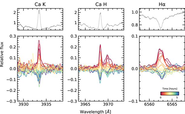
Figure 13. Spectroscopic activity indicators during the transit of 2021 Aug 7. The top panels show the median line profiles of Ca K, Ca H, and Hα from the HIRES spectra. The lower panels show the differences of each individual spectrum relative to the median spectrum. The bump in the red wing of Ca H is H . The spectra in the lower panels are smoothed for visualization purposes.
Download figure:
Standard image High-resolution imageThe expectation, however, is for the starspot-induced signals to be smooth, at worst with contributions at 0.5 Prot or 0.25 Prot (Klein & Donati 2020). We therefore fitted the RVs using the Hirano et al. (2010, 2011) models for the Rossiter−McLaughlin (RM) effect and allowed for an optional linear and quadratic trend in time to fit the ≈250 m s−1 spot-induced trend. We followed the methodology developed by Stefansson et al. (2020). We allowed the sky-projected obliquity, the projected stellar equatorial velocity, and the Gaussian dispersion of the spectral lines to vary, and fixed the limb darkening using the V-band tabulation from Claret & Bloemen (2011). We assumed a Gaussian prior on  and a/R⋆ from Table 1, and also allowed for a white-noise jitter term to be added in quadrature to the measurement uncertainties. We used a 15 minute exposure time to numerically evaluate the model.
The quadratic model with the RM effect is shown in Figure 8; the jitter term is incorporated in the model uncertainties, but not the plotted measurement uncertainties. The plotted measurement uncertainties are the internal uncertainties on the RVs (≈13 m s−1), and are dominated by the  broadening. However, between exposures, the RVs show significant additional scatter that is not captured by the slow quadratic trend. The white-noise jitter for this particular model is
  m s−1, which is comparable to the expected RM anomaly of
  , assuming a perfectly aligned orbit.
The presence of this additional scatter prevents a convincing detection of the RM effect. The reason can be understood via model comparison. If we compare the model with a quadratic trend and the RM effect against a model with a linear trend and the RM effect, or even a model with no RM effect at all, then the respective Bayesian Information Criterion (BIC) values are as follows.

There is therefore no evidence to prefer the model with the RM effect against a model that only accounts for the stellar variability. The "only quadratic" model does particularly well because it can inflate the jitter term to account for scatter during the transit (even if the scatter contains astrophysics!), and it has fewer free parameters. However, we cannot justify a physical prior on the jitter term, because we do not understand the origin of the exposure-to-exposure scatter. As noted above, the velocity deviations from starspots are expected to have contributions at the stellar rotation frequency, or harmonics thereof. This jitter is present on the exposure timescale (15 minutes), which is only 0.4% of the stellar rotation period; it is not obvious that starspots would be the culprit.
The amplitudes of both the spot-induced trend and the jitter are somewhat larger than recent comparable measurements in systems such as au Mic (Palle et al. 2020), DS Tuc (Montet et al. 2020; Zhou et al. 2020), and TOI 942 (Wirth et al. 2021). One possible explanation for the jitter is that it is astrophysical in origin, and that it is caused by some novel process operating on the surface of Kepler 1627A. Another possibility is that our RV analysis underestimates our measurement uncertainties; in order to achieve the requisite time sampling the signal-to-noise ratio per resolution element in our spectra was 70–80, which is lower than desired for deriving high-precision velocities. In addition, the rapid rotation of the star could affect accuracy of the uncertainties from the velocity extraction. Observations at higher signal-to-noise ratios are necessary to distinguish these two possibilities, and remain worthwhile in order to clarify the orbital geometry of Kepler 1627Ab. Useful next steps would include transit observations with a stabilized spectrograph in the optical (e.g., Gibson et al. 2016; Seifahrt et al. 2018), or in the near-infrared (e.g., Feinstein et al. 2021).
Appendix D: Flare Analysis
In addition to the 3.9 years of long cadence data, short cadence (1 minute) Kepler observations were acquired over 97.7 days during Quarter 15. The short cadence light curve shows a higher rate of flaring than visible in the long cadence data (Figure 14). We analyzed the short cadence light curve and its flares according to the following procedure.
- 1.Fit the starspot-induced variability using a Gaussian Process with a SHOTerm kernel, a white-noise jitter term, and the mean flux.
- 2.Select points more than twice the median absolute deviation from the residual, and exclude them from the light curve (these points include the flares). Repeat Step 1.
- 3.Using the residual from Step 2, identify all flares, requiring them to be at least 20 cadences apart, at least seven median absolute deviations above the median baseline, and lasting at least two cadences in duration. Build the mask spanning these times, from 5 minutes before each flare begins to 2.5 minutes after the final flare cadence. Repeat Step 1 a final time.
The final step of flare identification and fitting was performed using altaipony (Davenport 2016; Ilin et al. 2021). The analytic flare model is from Davenport et al. (2014) and it parameterizes the flare with a start time, an exponential lag time, and an amplitude.
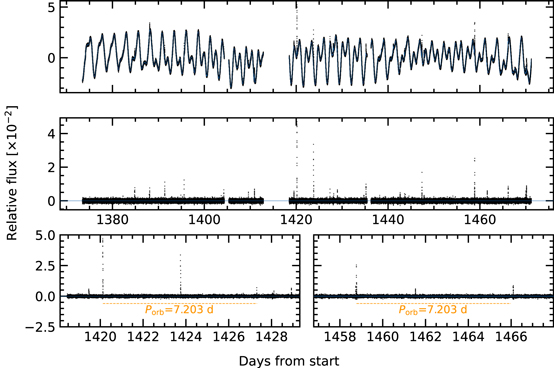
Figure 14. Flares in Kepler 1627. Top: the 1 minute cadence Kepler data (black points) are shown with a stellar variability model superposed (blue line). Middle: residual after subtracting the stellar variability model. Flares appear as spikes. Bottom: zooms of the brightest and third-brightest flares. A timing coincidence—that both flares have "successors" approximately one planetary orbital period after the initial event—is emphasized.
Download figure:
Standard image High-resolution imageThere were Nf = 24 flares that exceeded 0.5% in relative flux during the short cadence observations. These 24 flares spanned a total of 6.5 hr (∼15 minutes per flare). Inspecting the data, we noticed a coincidence in the flare arrival times. The coincidence is that despite the low flare duty cycle, one orbital period after the brightest flare, a second flare followed. This and a similar event are shown in Figure 14. The timing error is good to a ≈0.2% difference from the orbital period, which given the duty cycle seems a priori unlikely. If we consider flares falling within 2% of the planet's orbital period after a previous flare, then 4 of the 24 flare events have candidate "successors."
As with any coincidence, if one does not have a firm prediction, it is difficult to assess whether a surprise is statistically significant. Since our surprise was specifically at the interarrival time of certain flares coinciding with special time intervals, we performed the following analysis. First, we considered all unordered pairs of flares. For N flares there are  such pairs (for our case, 276 pairs). We then compared the distribution of the pair separations against that of a Poisson distribution. Specifically, we drew Nf = 24 samples from a Poisson distribution with λ = Δt/Nf, for Δt = 97.7 days the total duration of the observations, and repeated the draw 103 times with unique random seeds.
Figure 15 shows the results. The vertical lines in the figure show the planetary orbital period, the synodic period  , and linear combinations thereof. The tidal period (half the synodic period) is not shown. The bins are logarithmically spaced to give 100 bins between the minimum and maximum ordinate values. The gray bands express the range of values observed from the Poissonian draws. While it does seem like an odd coincidence for peaks in the observed flare arrival time distribution to coincide with the locations of these "special intervals," the statistical evidence for a non-Poissonian process driving the flares does not seem especially overwhelming. More quantitatively, the peaks observed at the orbital and synodic periods are within the ±2σ range of a Poissonian process, and those at Porb + Psyn and Porb + 2Psyn are only slightly above this range. With that said, future analyses of these data by investigators with more knowledge of this topic could very well yield more quantitative insights. Such analyses should keep in mind an important caveat: the amplitude distribution of M-dwarf flares extends up to many times the quiescent flux (see Figure 7 of Günther et al. 2020). A flare on Kepler 1627B producing double its quiescent white-light flux would yield a ≈1% apparent amplitude. Such flares could represent a significant fraction of those in the Kepler observations.
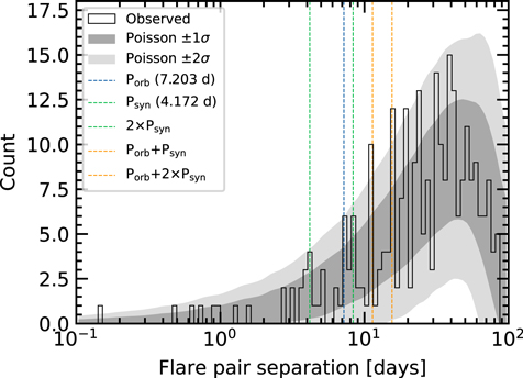
Figure 15. Statistics of interflare arrival times. Twenty-four flares were recorded with amplitudes exceeding 0.5% over the 97.7 days of short cadence observations. The histogram of the time intervals between every possible pair of flares is shown in black. Some plausibly important timescales for star−planet interactions, namely the planetary orbital period and synodic period (the orbital period as seen from the rotating stellar frame) are shown along with their linear combinations. Monte Carlo draws from a Poisson distribution are shown with the gray bands. While peaks in the observed distribution do coincide with some of the "special periods," the statistical evidence for a non-Poissonian process driving the flares does not clear the 5σ threshold.
Download figure:
Standard image High-resolution image
Footnotes
- 18
https://stilism.obspm.fr/, accessed 2021 Sep 25.
- 19
For a description of the renormalized unit weight error (RUWE), see the GAIA DPAC technical note http://www.rssd.esa.int/doc_fetch.php?id=3757412.
- 20
Our exploration of the PARSEC and MIST isochrone models over a grid of ages, metallicities, and reddenings yielded the best agreement for this ≈38 Myr age as well, given [Fe/H] = +0.1 and AV = 0.2 (Bressan et al. 2012; Choi et al. 2016); this preferred CAMD reddening is higher than the Lallement et al. (2018) value by a factor of two.
- 21
Our transit fitting yields e < 0.48 at 2σ; the constraints on the eccentricity are not particularly strong.
- 22