


Abstract
In this paper, we introduce an approach wherein the Weather Research and Forecasting (WRF) model is coupled with the bulk aerodynamic method to estimate the surface layer refractive index structure constant (Cn2) above Taishan Station in Antarctica. First, we use the measured meteorological parameters to estimate Cn2 using the bulk aerodynamic method, and second, we use the WRF model output parameters to estimate Cn2 using the bulk aerodynamic method. Finally, the corresponding Cn2 values from the micro-thermometer are compared with the Cn2 values estimated using the WRF model coupled with the bulk aerodynamic method. We analyzed the statistical operators—the bias, root mean square error (RMSE), bias-corrected RMSE (σ), and correlation coefficient (Rxy)—in a 20 day data set to assess how this approach performs. In addition, we employ contingency tables to investigate the estimation quality of this approach, which provides complementary key information with respect to the bias, RMSE, σ, and Rxy. The quantitative results are encouraging and permit us to confirm the fine performance of this approach. The main conclusions of this study tell us that this approach provides a positive impact on optimizing the observing time in astronomical applications and provides complementary key information for potential astronomical sites.
Export citation and abstract BibTeX RIS

Original content from this work may be used under the terms of the Creative Commons Attribution 3.0 licence. Any further distribution of this work must maintain attribution to the author(s) and the title of the work, journal citation and DOI.
1. Introduction
Finding optimal locations for large-aperture telescopes is a goal of astronomy. The main factors affecting the performance of ground-based astronomical telescopes are sky background, transmittance, and optical turbulence. Atmospheric turbulence is the major reason for the serious decline in imaging quality of optical telescopes (e.g., Tatarskii 1961; Chiba 1971), and the intensity of the atmospheric turbulence is usually described by the refractive index structure constant, Cn2.
The Antarctic plateau is the highest potential site at present, due to its extremely low temperature, dryness, and high altitude (more than 2500 m), joined to the fact that the optical turbulence there seems to be concentrated in a thin surface layer. The South Pole is the first site equipped with an observatory in the internal Antarctic plateau in which measurements of the Cn2 have been done (Marks et al. 1996, 1999), and analysis shows a highly turbulent boundary layer (0–220 m) coupled with strong temperature inversion, wind shear, and a very stable free atmosphere. The first astronomical seeing (ε) monitoring was made with the Differential Image Motion Monitor instrument at the Antarctic plateau site Dome C in 2002 December on the bright star Canopus (α Eri) during the daytime (Aristidi et al. 2003). A joint observation was conducted using the Multi-aperture Scintillation Sensor and Sound Detection And Ranging for experiments on seeing in 2004, and it indicated that the average seeing above 30 m at Dome C was 0.27 arcsec (Lawrence et al. 2004). This was followed by a series of studies, which were done with different instrumentations, to support the assessment of integrated seeing (Aristidi et al. 2005, 2009), the vertical distribution of Cn2 (Trinquet et al. 2008), and, using sonic anemometers, Cn2 in the surface layer at Dome C (Aristidi et al. 2015).
Since systematic direct measurements of Cn2 for many climates and seasons are not available, especially in severe environments, e.g., the Antarctic plateau, an indirect approach has been developed in which Cn2 can be calculated from the mesoscale atmospheric model (Meso-Nh) output. The comparison of the atmospheres above the South Pole, Dome C, and Dome A has been performed, with the result that Dome C shows the worse thermodynamic instability conditions compared to those predicted above the South Pole and Dome A above 100 m (Hagelin et al. 2008). More recently, the validation of the model above Dome C with supporting measurements has been done (Lascaux et al. 2009, 2010), and the model results match the measurements almost perfectly. Masciadri et al. provide the first homogeneous estimate, done with comparable statistics of the optical turbulence developed in the entire 22 km above the ground at Dome C, South Pole, and Dome A (Masciadri et al. 2010), and the ability of the Meso-NH model to discriminate between different optical turbulence behaviors has been confirmed. A later study was done in two other potential astronomical sites in Antarctica, Dome A and the South Pole, to investigate the ability of the model to discriminate between different turbulence conditions, and it is evident that the three sites have different characteristics with regard to the seeing and the surface layer thickness (Lascaux et al. 2011).
On account of the various ground-based optical application requirements, in a previous study, Qing et al. used the Monin–Obukhov Similarity (MOS) theory to estimate the surface layer Cn2 over the ocean (Qing et al. 2016). The MOS theory provides a rigorous scientific basis to estimate Cn2 from routine meteorological parameters in the surface layer; please refer to Davidson et al. (1981), Kunkel & Walters (1983), Hutt (1999), Frederickson et al. (2000), and references therein. In this paper, we use a simple approach to investigate the surface layer Cn2 above Taishan Station in Antarctica, and we focus on demonstrating the accuracy of this method. The corresponding Cn2 values measured by a micro-thermometer from a field campaign of the 30th Chinese National Antarctic Research Expedition (CHINARE) are used to validate the estimated values from this method. In addition, we analyzed the results of the bias, root mean square error (RMSE), bias-corrected RMSE (σ), correlation coefficient (Rxy), and contingency tables (Wilks 1995; Thornes & Stephenson 2001; Lascaux et al. 2015) between estimated Cn2 values and measured Cn2 values.
The plan of this paper is as follows: in Section 2, we give a brief overview of the WRF model configuration and in situ measurement system. Section 3 shows the temporal evolution of routine meteorological parameters. The theoretical background for estimating Cn2 is detailed in Section 4, and the temporal evolution of Cn2 is shown in Section 5. In Section 6, we present an independent analysis of the model performances using statistical operators, cumulative distributions, and contingency tables. In Section 7, some discrepancies between the estimations and the measurements, which may be caused by the uncertainty in the standard version of the MOS theory, are discussed. Final conclusions are drawn in Section 8.
2. Brief Overview of the In Situ Measurement System and Numerical Simulation
2.1. Principles of the In Situ Measurement System
The Taishan station (73°51' S, 76°58' E, at altitude 2621 m) in Antarctica is located on Princess Elizabeth Land between the Chinese Antarctic Zhongshan and Kunlun stations. The Antarctic mobile atmospheric parameter measurement system (Tian et al. 2015) includes a data logger, three-dimensional ultrasonic anemometer, micro-thermometer, temperature and relative humidity (RH) probe, wind speed and direction sensors, 485 communication modules, a power module, and a 3 m tower, which are shown in Figure 1. The main technical indicators of the in situ measurement system are shown in Table 1.
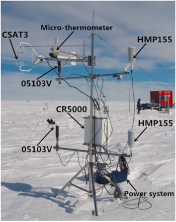
Figure 1. Mobile atmospheric parameter measurement system installed above Taishan Station in Antarctica.
Download figure:
Standard image High-resolution imageTable 1. Main Technical Specifications of the In Situ Measurement System
| Instrument | Model | Country | Measuring Element | Accuracy |
|---|---|---|---|---|
| Micro-thermometer | MT1 | China | Optical turbulence (Cn2) | 3E -18 |
| uz ≤ ± 0.04 | ||||
| Ultrasonic Anemometer | CSAT3 | USA | Three components of wind speed | uy ≤ ± 0.04 |
| uz ≤ ± 0.02 | ||||
| Temperature and Humidity Probe | HMP155 | Finland | Temperature | ≤± 0.5 |
| Relative humidity | ± 1% | |||
| Wind Speed and Direction Sensors | 05103V | USA | Wind speed | ± 0.3 |
| Wind direction | ± 3 |
Note. Note that the units of the parameters are °C for temperature, m s−1 for wind speed, degrees for wind direction, percent for relative humidity, and m for Cn2.
Download table as: ASCIITypeset image
The refractive index structure constants (Cn2, in units of  ), measured by the micro-thermometer, are deduced from a pair of horizontally separated micro-temperature probes. For visible and near-infrared wavelengths, the refractive index fluctuation is mainly caused by temperature fluctuation, and Cn2 can be directly related to the corresponding temperature structure constant (CT2) as follows (Marks et al. 1996; Cherubini & Businger 2012):

where T is the air temperature (K) and P is the air pressure (hPa). CT2 is defined as the constant of proportionality in the inertial subrange form of the temperature structure function DT(r). In the inertial subrange of the atmospheric turbulence, CT2 is given in Kolmogorov form (Pant et al. 1999) as follows:


where  and
and  denote the position vector, r is the magnitude of
  ,
,  represents the ensemble average, and l0 and L0 are the inner and outer scales of the atmospheric turbulence, respectively, and have units of m.
The platinum probe has a linear resistance–temperature coefficient, and it responds to an increase in atmospheric temperature with an increase in resistance. The two probes are the legs of a Wheatstone bridge, and the resistance of the probe is very nearly proportional to temperature, and thus temperature change is sensed as a voltage imbalance in the bridge. The micro-thermometer system provides CT2 data by measuring mean square temperature fluctuations (Equation (2)), and thus Cn2 data can be acquired from Equation (1). In our case, a 10 μm diameter platinum wire has the equivalent noise of about 0.002 K, and the observed Cn2 equivalent resolution is 3 × 10⁻¹⁸  (Wu et al. 2015).
2.2. WRF Model Configuration
The WRF model is a state-of-the-art mesoscale atmospheric model used for both professional forecasting and atmospheric research. It was developed by the National Centers for Environmental Prediction (NCEP) and the National Center for Atmospheric Research (NCAR), both in the United States. Details of the governing equations, transformations, and grid adaptation are given in the User's Guide, http://www2.mmm.ucar.edu/wrf/users/.
In this study, the initial data (at  horizontal resolution) are released every 6 hr by the NCEP (the final analysis or FNL; https://rda.ucar.edu/datasets/ds083.2/). We used grid-nesting techniques, which use different embedded domains of digital elevation models extended on increasingly smaller surfaces, with increasing horizontal resolution but with the same vertical grid (Stein et al. 2000). In a previous study (Masciadri & Lascaux 2012; Lascaux et al. 2015; Masciadri et al. 2017), Masciadri and Lascaux used three embedded domains, where the horizontal resolution of the innermost domain is 500 m, to obtain the most relevant parameters related to optical turbulence (Cn2, seeing ε, isoplanatic angle
  , and wavefront coherence time
  ). In this work, the three embedded domains (the horizontal resolution of the innermost domain is 500 m) and the vertical resolution are satisfactory to estimate the surface layer Cn2 according to the validation experiment. We set the WRF model with a conventional 5:1 nesting scheme for two-way interactive domains; this allows the largest domain to cover an area of approximately 1125 km by 1125 km at a 12.5 km grid resolution. It is then nested down to 2.5 km around the Antarctic Taishan station and then down to 0.5 km at the location of the Antarctic mobile atmospheric parameter measurement system. We also note that the model configuration we selected is suitable for performing Cn2 estimates using relatively cheap hardware. The basic simulation parameters settings are listed in Table 2 and detailed in the User's Guide. The Antarctic Plateau map is shown in Figure 2, where the red solid circle stands for the center of the simulation domain.
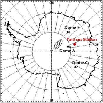
Figure 2. Antarctic Plateau map. The site of Taishan Station is marked by a red solid circle. The black solid circles represent Dome A, Dome C, and Dome F.
Download figure:
Standard image High-resolution imageTable 2. WRF Model Grid-nesting Configuration for the Simulation
| Domain | Grid Points |
 (km) (km) |
Domain Size (km2) |
|---|---|---|---|
| Domain 1 | 90 × 90 | 12.5 | 1125 × 1125 |
| Domain 2 | 75 × 75 | 2.5 | 187.5 × 187.5 |
| Domain 3 | 45 × 45 | 0.5 | 22.5 × 22.5 |
Note. The second column shows the number of horizontal grid points, the third column shows the horizontal resolution ( ), and the fourth column shows the horizontal surface covered by the model domain.
Download table as: ASCIITypeset image
The WRF model provides a large number of atmospheric parameters (such as the temperature, RH, wind speed, direction, etc.), which depend upon the parameterization schemes that have been chosen for the simulation, most of which are self-explanatory although some require additional information. The main physical schemes are listed in Table 3, and the parameterization schemes are now included in the official WRF release and explained as follows (Skamarock et al. 2006):
- 1.The microphysics process uses the WRF Single-moment 5 class (WSM-5) scheme, which is a slightly more sophisticated version of the WRF Single-moment 3 class (which contains three kinds of water materials: water vapor, cloud water or cloud ice, rainwater or snow) that allows for mixed-phase processes and super-cooled water.
- 2.The longwave radiation uses the Rapid Radiative Transfer Model (RRTM) scheme, an accurate scheme that uses look-up tables for efficiency and accounts for multiple bands and microphysics species. The longwave process is caused by water vapor, ozone, carbon dioxide, and other gases, as well as by the optical depth of cloud.
- 3.The shortwave radiation uses the Goddard scheme, a two-stream multiband scheme using ozone from climatology and cloud effects. The Goddard scheme is suitable for cloud-resolution models.
- 4.The surface layer uses the Eta similarity scheme, which is based on Monin–Obukhov with Zilitinkevich thermal roughness length and standard similarity functions from look-up tables.
- 5.The planetary boundary layer uses the Mellor–Yamada–Janjić (MYJ), scheme, which may be used to forecast turbulent energy using the one-dimensional prognostic turbulent kinetic energy scheme with local vertical mixing.
Table 3. Settings of the Main Physical Schemes
| Physical Scheme | Settings |
|---|---|
| Microphysics Process | WSM-5 class |
| Longwave Radiation | RRTM |
| Shortwave Radiation | Goddard |
| Boundary Layer | Eta similarity |
| Planetary Boundary Layer | MYJ |
Download table as: ASCIITypeset image
2.3. Data Selection
The site testing experiments were carried out during the 30th CHINARE. Two levels (0.5 m and 2 m above ground) of air temperature, RH, and wind speed and direction, and one level (2 m above ground) of air pressure, surface temperature, Cn2, and other atmospheric parameters can be measured by the Antarctic mobile atmospheric parameter measurement system at the same time, which is close to the center grid point of the simulation domain. We should note that the ensemble average time of the micro-thermometer is 10 seconds, while the WRF model outputs result at 10 minute intervals owing to the model configuration limitation. The in situ measured values are averaged over the same interval to match up with the simulated ones for a meaningful comparison.
To actually validate the results between simulation and measurement, it requires the in situ measurements to be matched up with the model output at the corresponding time period. The initial field data (FNL) we used was released at the NCEP Web site 19:00:00 UTC before the start of each simulation, with a simulation time of 72 hr.
3. Temporal Evolution of Routine Meteorological Parameters for the Model and In Situ Measurements
Before estimating Cn2, the diurnal features of the temperature, wind speed and direction, and RH simulated using the WRF model and measured by the mobile atmospheric parameter measurement system in the surface layer were investigated and are shown in Figures 3(a)–(d), respectively. In terms of the diurnal features of the temperature, the results agree with the model, while the range of abilities of the simulations, shown in Figure 3(a), is relatively larger than that of the measurements. From Figure 3(b), the surface layer wind speed is relatively stable, yet the simulated wind speed is consistent with the measured one in trend in general. Up to now, few studies have aimed to analyze in depth the quality of the simulation of the wind direction using the mesoscale model. For ground-based astronomy, it is more important to know the wind direction when the wind is strong. According to Figure 3(c), the diurnal features of the wind direction are obviously stable, and the simulated values are very well consistent with the measured ones. In addition, the diurnal features of the RH are obvious, whereas the simulated values are consistent with the measured values in trend in general, seen in Figure 3(d).
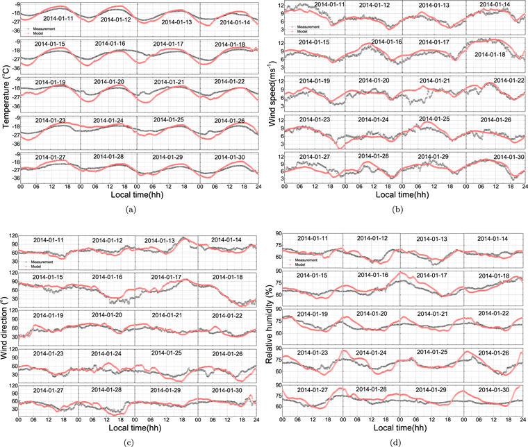
Figure 3. Diurnal features of the surface layer meteorological parameters for the model and in situ measurements above Taishan Station in Antarctica (20 days overall, at 2 m high). The red open circles and the black open circles represent the model and measurement, respectively. Diurnal features for (a) temperature, (b) wind speed, (c) wind direction, and (d) relative humidity.
Download figure:
Standard image High-resolution imageOverall, when looking at the diurnal features of routine meteorological parameters, the model very nicely captures the timing and the magnitude of the evolution of the routine meteorological parametersthroughout the entire month of January, although larger uncertainties were found in several of the days. It is promising that the simulations agreed with the measurements, for the terrain of Antarctica is the most homogeneous on the planet, even smoother than the ocean. Therefore, the desirable features of the model have demonstrated its potential to accurately simulate routine meteorological parameters in the surface layer based on a long time confirmation, and it provides a basis to estimate Cn2 in the surface layer.
4. Theoretical Background for Estimating the Atmospheric Refractive Index Structure Constant (Cn2)
4.1. Brief Overview of Cn2
The refractive index structure constant (Cn2) is an important parameter in the study of electromagnetic wave propagation in the atmospheric surface layer. Because turbulent fluctuations of the atmospheric refractive index ( ) at a given wavelength (λ) are related to fluctuations in the temperature (T) and humidity (q) by
  , it is possible to estimate Cn2 from the meteorological parameters (Andreas 1988; Andreas et al. 1998; Qing et al. 2016). For Kolmogorov turbulence, which is similar to the atmospheric refractive index structure constant Cn2, the temperature structure constant (CT2), specific humidity structure constant (Cq2), and the temperature–humidity cross-structure constant (CTq) can be defined as


where  and
and  denote the position vector, r is the magnitude of
  ,
,  represents the ensemble average, and l0 and L0 are the inner and outer scales of the atmospheric turbulence, respectively.
These similarity relations suggest that Cn2 also exhibits the MOS theory, and Cn2 can be defined in terms of CT2, Cq2, and CTq as (Gossard 1960; Wesely 1976; Hill et al. 1980)

For a chosen electromagnetic wavelength and a given set of meteorological conditions, the coefficients A and B are constant. For practical purposes, at the wavelength of interest of 0.55 μm, A =  P/T2 and
  . The first term on the right-hand side of Equation (4) represents the refractive index fluctuations caused by temperature fluctuations and is always positive, the second term represents the correlation of temperature and humidity fluctuations and can be positive or negative, while the third term represents humidity fluctuations and is always positive.
4.2. Bulk Aerodynamic Method for Estimating Cn2
The structure constants CT2, Cq2, and CTq can be expressed in terms of T* and q* as follows (Fairall et al. 1980; Fairall & Larsen 1986):


where z/L is an (dimensionless) indicator of the state of stability of the atmospheric boundary layer with respect to buoyancy, z is the height, and L is the Monin–Obukhov length.  is the temperature–humidity correlation coefficient. We use a value of 0.5 for
  when
when  , and a value of 0.8 when
  in this work (Frederickson et al. 2000). The similarity functions
  ,
,  , and
, and  are determined by experiment and are usually supposed to be
  . In this paper, the similarity function
  that we use is determined during a field campaign in Kansas (Wyngaard et al. 1971):

Subsequently, substituting Equation (5) into Equation (4) gives a Cn2 expression in terms of T*, q*, and L:

According to MOS theory, it is possible to express the scaling parameters for temperature (T*), specific humidity (q*), and wind speed (u*) as follows:


where  is the average wind speed at height z,
  , and
, and  . T(z) and q(z) are the average air temperature and average specific humidity at height z, respectively. Ts and qs are the surface temperature and specific humidity, respectively. The drag coefficient (CD), sensible heat flux coefficient (CH), and moisture flux coefficient (CE) are all from experiment, and their values are given below (Pond et al. 1971; Smith & Banke 1975; Friehe & Schmitt 1976; Friehe 1977):


For the parameterization of the Monin–Obukhov length L, the expression for L is given by the two  ranges as follows (Deardorff 1968):
Therefore, the values of U(z), T(z), and q(z), as well as of Ts and qs, are given by the WRF model first, and then the air–surface difference for temperature ( ), specific humidity (
 ), and average wind speed (
 ) is calculated. We can obtain u*, T*, and q* by solving Equations (8)–(9), and obtain z/L by solving Equation (10). Finally, it is simple to estimate Cn2 from Equations (6)–(7).
5. Temporal Evolution of Cn2 from the Estimations and Measurement
First, we use the measured meteorological parameters to estimate Cn2 based on the bulk aerodynamic method, and second, we use the WRF model output meteorological parameters to estimate Cn2 with this method in a similar manner. Finally, a comparison between the Cn2 estimated with the WRF model output meteorological parameters (as well as the Cn2 estimated from the measured meteorological parameters) and the Cn2 measured by the micro-thermometer was performed. From this point until the end of the paper, we write Cn2(Model) instead of "Cn2 estimated from the WRF model output meteorological parameters," Cn2(Estimate) instead of "Cn2 estimated from the measured meteorological parameters," and Cn2(Micro-thermometer) instead of "Cn2 measured by the micro-thermometer," and will be used hereafter.
The temporal evolution of Cn2(Model), Cn2(Estimate), and Cn2(Micro-thermometer) in the surface layer are depicted in Figure 4. One can see that Cn2(Model) agrees reasonably well with Cn2(Micro-thermometer) in trend and magnitude in general. Furthermore, this approach qualitatively captures several "sharp drop-offs" of Cn2 during the morning and evening transitions in a faithful manner, which are clearly visible in this plot. In some cases, these "sharp drop-offs" are estimated to be earlier by about one hour. Moreover, the Cn2(Model) values tend to be overestimated slightly while having relatively better performance in the low range of Cn2. Quite interestingly, some specific features of the surface layer Cn2 above Taishan Station in Antarctica have been displayed in Figure 4, where the diurnal variations of the estimated Cn2 and that of the measured Cn2 are all obvious, with the peak value of Cn2 not always the strongest at about 12:00 (local time). Due to the high altitude, thin air, high latitude, and reflection of solar radiation on the ice surface, the difference in temperature between the two surface layers is in contrast to that of land, resulting in characteristics of the atmospheric turbulence intensity different from those of inland areas. When solar radiation and surface radiation gradually balance one another, the ground temperature and air temperature become consistent and atmospheric stratification is in a neutral state, which has little impact on the generation and development of optical turbulence.
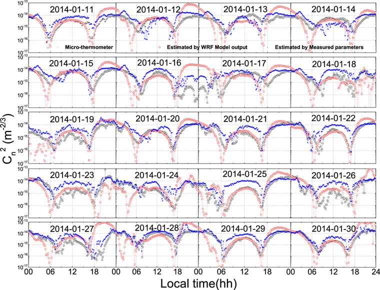
Figure 4. Temporal evolution of the surface layer Cn2 from the estimations and in situ measurement (20 days overall, at 2 m high). The red open circles represent the Cn2 estimated from the WRF model output, the blue crosses represent the Cn2 estimated from the measured meteorological parameters, and the black open circles represent the Cn2 measured by the micro-thermometer. The time resolution of the dots in the figure is 10 minutes.
Download figure:
Standard image High-resolution imageFor these reasons, the optical turbulence is weakest during the day in most cases. Our approach reflects the diurnal variation of the surface layer optical turbulence above Taishan Station in Antarctica accurately. The estimations are somewhat poorer than the agreement with the measurements, but are satisfactory for most purposes. Still, some discrepancies between the estimations and the measurements may be caused by the uncertainty in the standard MOS theory. In addition, the valley spikes of the estimated Cn2 occur when atmospheric stratification is in a neutral state, so there still exists some room for improvement. In Section 7, some discrepancies between the estimations and the measurements are discussed.
6. Statistics and Uncertainty Analysis
6.1. Statistical Operators: Bias, RMSE,  , and Rxy

Several statistical operators—the bias, the RMSE, and the correlation coefficient (Rxy)—have been used to assess the accuracy of this approach, which follows the same framework as Lascaux et al. (2015):
with  , where Xi are the individual measured values, Yi the individual values simulated by the WRF model at the same time, N is the number of times for which a couple (Xi, Yi) is available, and
  and
and  stand for the average values of the measured and simulated parameters, respectively. From the bias and RMSE, we deduce the bias-corrected RMSE (σ):

σ represents the error of the model once the systematic error (the bias) is removed.
Because the wind direction is a circular variable, we define  for the wind direction as
The temporal evolution of the bias (model minus measurement), RMSE, σ, and Rxy between the measurement and estimations for the relevant meteorological parameters in the surface layer is shown in Figures 5(a)–(f). The comparisons between measurement and estimations are shown to provide a valuable picture of the surface layer temporal evolution of the bias, RMSE, σ, and Rxy for the relevant meteorological parameters at the Taishan Station in Antarctica.
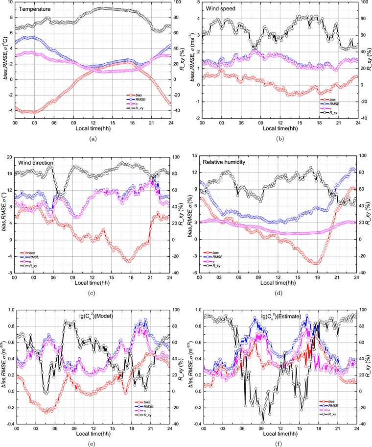
Figure 5. Temporal evolution of the bias, RMSE, σ, and Rxy for the model and in situ measurement in the surface layer (model minus in situ measurement, 20 days overall, at 2 m high). Temporal evolution of the statistical operators for (a) temperature, (b) wind speed, (c) wind direction, (d) relative humidity, (e)  (Model), and (f)
  (Estimate).
Download figure:
Standard image High-resolution imageLooking at Figure 5(a) for temperature, the bias is well below 4 °C (at some times well below 1 °C), and it is even more satisfactory that the RMSE is basically always lower than 1 °C. Therefore, we obtain promising RMSE, σ, and Rxy values.
Figure 5(b) shows the temporal evolution of the statistical operators for wind speed. We can see that the bias is well below 1 m s−1 (at some times well below 0.5 m s−1), and the RMSE and σ are basically always lower than 2 m s−1, and Rxy is mostly higher than 50% (at some times well above 80%). The values of the bias, RMSE, σ, and Rxy are satisfactory.
Figure 5(c) shows the temporal evolution of the statistical operators for wind direction. We can see that the bias is well below 8°, and the RMSE and σ are basically always lower than 16°, and Rxy is mostly higher than 60% (at some times well above 90%). These are promising results demonstrating the desirable ability of the model to predict the general wind direction.
Figure 5(d) shows the temporal evolution of the statistical operators for RH. We can see that the bias is well below 9%, and the RMSE and σ are basically always lower than 12%, and Rxy is mostly higher than 50% (at some times well above 80%).
Figure 5(e) shows the temporal evolution of the statistical operators for  estimated using the WRF model in the surface layer, and we obtain satisfactory bias, RMSE, σ, and Rxy values. Moreover, the bias is well below 0.5
  , and the RMSE and σ are basically always lower than 0.8
  , while during the morning and evening transitions, Rxy is close to 0 (but well above 50% most times).
Figure 5(f) shows the temporal evolution of the statistical operators for  estimated using the measured parameters in the surface layer, and we also obtain promising bias, RMSE, σ, and Rxy values. What's more, the bias is well below 0.6
  ; at the same time, the RMSE and σ are basically always lower than 0.9
  , while during morning and evening transitions, Rxy is close to 0 (but well below 0 most times).
The values of the bias, RMSE, σ, and Rxy for the temperature, wind speed and direction, RH, and  in the surface layer are tabulated in Table 4 for all 20 days. FromTable 4, the bias, RMSE, and σ are very small, especially for the wind speed, RH, and Cn2, while the Rxy values are relatively large and the Cn2 values estimated from the WRF model in the surface layer are promising. In addition, we present an analysis of the model performances in reconstructing the meteorological parameters day by day. We compute the bias, RMSE, σ, and Rxy for every single day (from the 20 day sample) for the temperature, wind speed and direction, RH, Cn2(Model), and Cn2(Estimate). We also calculate the cumulative distributions of the bias, RMSE, σ, and Rxy, including the median, and first and third quartiles; these are summarized in Table 5. As we have seen, the bias, RMSE, σ, and Rxy of the day-by-day analysis are slightly better than the bias, RMSE, σ, and Rxy of the overall statistics (Table 4).
Table 4. Values of the Bias, RMSE, σ, and Rxy of the Temperature, Wind Speed and Direction, Relative Humidity (RH), and Cn2 in the Surface Layer (Model minus In Situ Measurement, 20 Days Overall, at 2 m High)
| Statistical Operator | Temperature | Wind Speed | Wind Direction | Relative Humidity |
 (Model) (Model) |
 (Estimate) (Estimate) |
|---|---|---|---|---|---|---|
| Bias | 1.6 | 0.1 | 2 | 2 | 0.1 | 0.3 |
| RMSE | 3.6 | 1.5 | 11 | 6 | 0.6 | 0.5 |
| σ | 3.2 | 1.5 | 11 | 6 | 0.6 | 0.4 |
| Rxy | 83.8% | 75.8% | 84.3% | 71.8% | 62.7% | 66.8% |
Note. Note that the units of the parameters are °C for temperature, m s−1 for wind speed, degrees for wind direction, percent for relative humidity, and m for
for  .
.
Download table as: ASCIITypeset image
Table 5. Median Bias, RMSE, σ, and Rxy of the Temperature, Wind Speed, and Direction, Relative Humidity, and Cn2 in the Surface Layer for a Single Day (Model minus In Situ Measurement, 20 Day Sample, at 2 m High)
| Statistical Operator | Temperature | Wind Speed | Wind Direction | Relative Humidity |
 (Model) (Model) |
 (Estimate) (Estimate) |
|---|---|---|---|---|---|---|
| Bias |

|

|

|

|

|

|
| RMSE |

|

|

|

|

|

|
| σ |

|

|

|

|

|

|
| Rxy |

|

|

|

|

|

|
Note. The subscripts and the superscripts show the first and third quartiles, respectively. Note that the units of the parameters are °C for temperature, m s−1 for wind speed, degrees for wind direction, percent for relative humidity, and m for  .
.
Download table as: ASCIITypeset image
6.2. Contingency Table
As mentioned in the introduction, we utilize a contingency table to investigate the relationship between the estimated values and measurements. A contingency table, which is a table with n × n entries that displays the distribution of model and measurement values in terms of frequencies or relative frequencies (Lascaux et al. 2015), allows for the analysis of the relationship between two or more categorical variables.
We list all of the different simple scores we will use in the paper from a generic 3 × 3 contingency table: percent of correct detections (PC), probability of detection (POD; in %), and extremely bad detection (EBD; in %). PC = 100% is the best score, and it corresponds to a perfect estimation. POD = 100% is the best score, which represents the proportion of measured values that have been correctly estimated with this approach. EBD represents the percent of the most distant values estimated with this approach from the measurements, and it is equal to 0% for a perfect estimation. In the case of a perfectly random estimation, all PODs will be equal to 33%, but PC = 33% and EBD = 22.2%. The model will be useful if these values perform better than those random cases (33% or 22.2%). These values are a good reference to evaluate the performance of this approach. We will write PODi instead of POD ( ) when event i is considered (Qing et al. 2016).
In this study, we decided to use climatological tertiles computed from the available measurements. We used 20 days of measurements, from 2014 January 11 to 2014 January 30. Tables 6–11 show the results of the contingency table for the temperature, wind speed and direction, RH, Cn2(Model), and Cn2(Estimate) in the surface layer, respectively.
6.2.1. Temperature
The first meteorological parameter reconstructed by the model that we have investigated is the temperature in the surface layer; it is tabulated in Table 6. We can observe that the PC by the model is very good, and the PC is up to 66.1%. Moreover, the EBD (1.9%) is very close to 0%, which is a sign that the model never produces extremely bad estimates for the temperature. We look at the POD of the temperature in a given interval; once again, the model demonstrates its accuracy. POD1 (temperature inferior to −25.1 °C) is 74.8%, POD2 (temperature between −25.1 °C and −19.5 °C) is 43.4%, and POD3 (temperature superior to −19.5 °C) is 91.2%. In all cases, the PC and PODi are much larger than 33% (the value for a random case), which confirms the goodness of the sim-ulation by the model. Thus, one could think of using the estimated temperature at the beginning of the night for the thermalization of the dome of the telescope.
Table 6.
3 × 3 Contingency Table for Temperature (in °C) above Taishan Station in Antarctica (20 Days Overall, at 2 m high),  m Configuration
| Intervals | Observations | ||||
|---|---|---|---|---|---|
| T ≤ −25.1 | −25.1 ≤ T ≤ −19.5 | T ≥ −19.5 | Total | ||
| T ≤ −25.1 | 910 | 0 | 4 | 914 | |
| −25.1 ≤ T ≤ −19.5 | 256 | 475 | 46 | 777 | |
| Model | T ≥ −19.5 | 50 | 620 | 519 | 1189 |
| Total | 1216 | 1095 | 569 | N = 2880 | |
Note. Total events = 2880; PC = 66.1%; EBD = 1.9%; POD1 = 74.8%; POD2 = 43.4%; POD3 = 91.2%.
Download table as: ASCIITypeset image
6.2.2. Wind Speed
Strong wind is indeed the main cause of vibrations of the primary mirror and adaptive secondary, which are critical elements of the adaptive optics (AO) system. In this section, we investigate the ability of the model to simulate the wind speed, as tabulated in Table 7. We observe that the PC (64.6%) is better than 33%. Moreover, the EBD (4.2%) is negligible. POD1 (wind speed inferior to 6.7 m s−1), POD2 (wind speed between 6.7 m s−1 and 8.4 ms−1), and POD3 (wind speed superior to 8.4 m s−1) are 71.1%, 48.7%, and 76.6%, respectively. In all cases, the PC and PODi are much larger than 33%. This demonstrates the ability of the model to simulate critical wind speed values for AO applications.
Table 7. Same as Table 6, but for Wind Speed (in m s−1)
| Intervals | Observations | ||||
|---|---|---|---|---|---|
| WS ≤ 6.7 | 6.7 ≤ WS ≤ 8.4 | WS ≥ 8.4 | Total | ||
| WS ≤ 6.7 | 693 | 212 | 48 | 953 | |
| 6.7 ≤ WS ≤ 8.4 | 210 | 509 | 153 | 872 | |
| Model | WS ≥ 8.4 | 72 | 325 | 658 | 1055 |
| Total | 975 | 1046 | 859 | N = 2880 | |
Note. Total events = 2880; PC = 64.6%; EBD = 4.2%; POD1 = 71.1%; POD2 = 48.7%; POD3 = 76.6%.
Download table as: ASCIITypeset image
6.2.3. Wind Direction
For an astronomer using ground-based facilities, it is more important to know the wind direction accurately when the wind is strong. As we already anticipated, the wind direction is the parameter that is most correlated to the seeing conditions above observatories. Moreover, experience shows that the most useful information in an astronomical context is typically identifying the direction from where the wind comes. Knowing in advance the main direction of the wind near the surface could allow the astronomer to anticipate the occurrence of a good or bad seeing night and to plan the observations consequently. We investigate the reconstruction of the wind direction by the model, as tabulated in Table 8. According to Figure 3(c), the wind direction is very stable, and it is centralized in the range 10°–120°, so a 3 × 3 contingency table is also used for wind direction. We observe that the PC (67.6%) is greater than 33%, and the EBD is 2.6%. POD1 (wind direction inferior to 48°) is 63.8%, POD2 (wind direction between 48°and 62°) is 55.6%, and POD3 (wind direction superior to 62°) is 86.3%. In all cases, the PC and PODi are much larger than 33%, which is a very positive result.
Table 8. Same as Table 6, but for Wind Direction (in °)
| Intervals | Observations | ||||
|---|---|---|---|---|---|
| WD ≤ 48 | 48 ≤ WD ≤ 62 | WD ≥ 62 | Total | ||
| WD ≤ 48 | 687 | 172 | 1 | 860 | |
| 48 ≤ WD ≤ 62 | 315 | 537 | 114 | 966 | |
| Model | WD ≥ 62 | 75 | 257 | 722 | 1054 |
| Total | 1077 | 966 | 837 | N = 2880 | |
Note. Total events = 2880; PC = 67.6%; EBD = 2.6%; POD1 = 63.8%; POD2 = 55.6%; POD3 = 86.3%.
Download table as: ASCIITypeset image
6.2.4. Relative Humidity
In practice, an astronomer needs to know if the humidity during the night is higher than 80%, the threshold where the dome must be closed and thus observations are not allowed. In this section, we investigate the reconstruction of the RH by the model, as tabulated in Table 9. We can observe that the PC (59.5%) is larger than 33%, and the EBD is 2.9%. POD1 (RH inferior to 65%) is 65.9%, POD2 (RH between 65% and 70%) is 38.1%, and POD3 (RH superior to 70%) is 83.6%. In all cases, the PC and PODi are much larger than 33%. Our results indicate that the model can give a positive simulation of the night's RH, which is useful for astronomers.
Table 9. Same as Table 6, but for Relative Humidity (in Percent)
| Intervals | Observations | ||||
|---|---|---|---|---|---|
| RH ≤ 65 | 65 ≤ RH ≤ 70 | RH ≥ 70 | Total | ||
| RH ≤ 65 | 610 | 340 | 26 | 976 | |
| 65 ≤ RH ≤ 70 | 260 | 443 | 104 | 807 | |
| Model | RH ≥ 70 | 56 | 380 | 661 | 1097 |
| Total | 926 | 1163 | 791 | N = 2880 | |
Note. Total events = 2880; PC = 59.5%; EBD = 2.9%; POD1 = 65.9%; POD2 = 38.1%; POD3 = 83.6%.
Download table as: ASCIITypeset image
6.2.5. Optical Turbulence (Cn2)
Finally, we investigate the estimation of the optical turbulence using this approach. The Cn2 estimated from the measured meteorological parameters is tabulated in Table 10, and the Cn2 estimated from the WRF model output is tabulated in Table 11. We observe that the PC (51.1%) for Cn2 estimated from the measured parameters is better than 33%, and the EBD is 6.9%. POD1 ( inferior to −14.8
  ) is 38.2%, POD2 (
 between −14.8
  and −14.3
  ) is 33.4%, and POD3 (
 superior to −14.3
  ) is 95.1%, while POD
 is much smaller than 33% (in Table 10).
Table 10.
Same as Table 6, but for Cn2 Estimated from the Measured Meteorological Parameters (in  )
)
| Intervals | Observations | ||||
|---|---|---|---|---|---|

|
−14.8 ≤ 
|

|
Total | ||

|
494 | 119 | 5 | 618 | |

|
604 | 288 | 30 | 922 | |
| Model |

|
195 | 456 | 689 | 1280 |
| Total | 1293 | 863 | 724 | N = 2880 | |
Note. Total events = 2880; PC = 51.1%; EBD = 6.9%; POD1 = 38.2%; POD2 = 33.4%; POD3 = 95.2%.
Download table as: ASCIITypeset image
Table 11.
Same as Table 6, but for Cn2 Estimated from the WRF Model Output (in  )
)
| Intervals | Observations | ||||
|---|---|---|---|---|---|

|
|

|
Total | ||

|
695 | 230 | 35 | 960 | |

|
241 | 513 | 189 | 943 | |
| Model |

|
108 | 165 | 704 | 977 |
| Total | 1044 | 908 | 928 | N = 2880 | |
Note. Total events = 2880; PC = 66.4%; EBD = 4.9%; POD1 = 66.6%; POD2 = 56.5%; POD3 = 75.9%.
Download table as: ASCIITypeset image
The PC (66.4%) for Cn2 estimated from the WRF model output is significantly better than 33%, and the EBD is 4.9%. POD1 ( inferior to −14.8
  ) is 66.6%, POD2 (
 between −14.8
  and −14.3
  ) is 56.5%, and POD3 (
 superior to −14.3
  ) is 75.9%. In all cases, the PC and PODi are much larger than 33% (see Table 11). In view of these points, the results for the Cn2 estimated from the WRF model output meteorological parameters are even better than the similar results estimated from the measured meteorological parameters. Hence, this proves the utility of this approach for estimating Cn2 in the surface layer.
7. Discussion
The Cn2 estimated from the WRF model coupled with the bulk method agrees with the Cn2 measured by the micro-thermometer overall; still, there are some discrepancies between the estimations and measurements.
- 1.The Cn2 value measured by the micro-thermometer could be considered as a "point" measurement at a spec-ific location, while the Cn2 estimated from the WRF model should be considered as the 10 minute statistical average over a 0.25 km2 area for the center of the simulation domain. Improvements are expected from the WRF model's finer horizontal grid resolution as well as time interval of the output meteorological parameters in subsequent work.
- 2.The form of the similarity function is very important to the accuracy of estimating Cn2 (Edson et al. 1991). The critical and reasonable form of is determined with a lot of difficulty; nevertheless, the structure is similar and only the coefficient is different. The form of cited in this paper was determined in the Kansas experiment in 1968 (Wyngaard et al. 1971), and also cited in Andreas's paper to estimate Cn2 over snow and sea ice (Andreas 1988). The bulk aerodynamic formulas are simple empirical parameterizations of the surface fluxes of momentum, sensible heat, and moisture in the boundary layer in terms of average surface layer variables. In this study, it was assumed that the coefficients CD, CH, and CE are independent of z/L (Friehe 1977), but Deardorff derived coefficients for the dependence of the coefficients on stability (Deardorff 1968). The noted uncertainties in the retrieval of the surface fluxes from the measurements point to the fact that the analysis of intermittent turbulence is still an ongoing research area. More numerous and accurate observations of wind, temperature, and humidity in the surface layer as well as measurements of the vertical transfer rates are needed to confirm and extend the present analysis.
- 3.The atmospheric turbulence is slightly impacted by the surroundings over open snow and sea ice surface layer above Taishan Station in Antarctica, but there still exist some uncertainties. The measurement height or the height where the Cn2 value was estimated with this approach may be above the constant flux layer in a region where the MOS theory is invalid when the surface layer can become very thin in very stable conditions (Mahrt 1999). The MOS theory seems difficult to circumvent, however, as it is at the basis of surface-flux calculation in numerical weather prediction models. Of course, more measured data are required under different stability conditions to test precisely the bulk aerodynamic formulas.


8. Summary and Conclusions
In this study, we focused on demonstrating the accuracy of the approach that couples the WRF model with the bulk aerodynamic method in reconstructing routine meteorological parameters (such as temperature, RH, wind speed and direction, etc.) and Cn2 in the surface layer. First, we use the WRF model output meteorological parameters and the measured meteorological parameters to estimate Cn2 based on the bulk method, and then we compared the Cn2 estimated with this approach and that measured by the micro-thermometer. To quantify the quality of this approach, we use a 20 day data set from a field campaign of the 30th CHINARE to thoroughly analyze the performance of this approach in simulating the main routine meteorological parameters and Cn2. The results we obtained on the validation samples are summarized in a nutshell.
For the routine meteorological parameters, the simulated ones are well consistent with the measured ones, and the model very nicely captures the timing and magnitude of the evolution of the routine meteorological parameters. Therefore, the desirable features of this model have demonstrated its potential to accurately simulate routine meteorological parameters in the surface layer. Moreover, the Cn2 estimated with this approach agrees reasonably well with that measured by the micro-thermometer and with some specific features, wherein the diurnal variations of the estimated Cn2 and the measured Cn2 are all obvious, with the peak value of Cn2 not always strongest at about 12:00 (local time). In addition, from the statistical operators and the 3 × 3 contingency tables, the bias, RMSE, σ, and Rxy of the day-by-day analysis are excellent. The PC and EBD are satisfactory, and the PODi are all greater than 33%.
The quantitative results indicate that the accuracy of this approach in reconstructing the routine meteorological parameters and Cn2 in the surface layer is satisfactory, and the results of this study guarantee a concrete practical advantage from the implementation of site testing for astronomical applications, though some room for improvement still exists. Our research will definitely take advantage of the fact that we have as many different reliable instruments as possible running simultaneously above a site because this permits us not only to better constrain the model but also to better quantify the uncertainty with which we can estimate the optical turbulence.
We sincerely acknowledge the anonymous reviewers for their valuable comments and suggestions, and gratefully thank NCAR for access to their meteorological data set. The authors wish to thank the Polar Research Institute of China for support, and the members of the 30th CHINARE team for their great help with the installation of the mobile atmospheric parameter measurement system. This work was supported by the Polar Science Innovation Fund for Young Scientists of the Polar Research Institute of China (grant No. CX20130201), the Natural Science Foundation of Shanghai (grant No. 14ZR1444100), the Chinese Polar Environment Comprehensive Investigation & Assessment Programs (grant Nos. CHINARE2013-02-03 and CHINARE2014-02-03), the Project funded by the China Postdoctoral Science Foundation (2017M622034), and was jointly supported by the National Natural Science Foundation of China (grant No. 41576185).