


Abstract
Because ion–neutral reaction cross sections are energy dependent, the distance from a cometary nucleus within which ions remain collisionally coupled to the neutrals is dictated not only by the comet's activity level but also by the electromagnetic fields in the coma. Here we present a 1D model simulating the outward radial motion of water group ions with radial acceleration by an ambipolar electric field interrupted primarily by charge transfer processes with H2O. We also discuss the impact of plasma waves. For a given electric field profile, the model calculates key parameters, including the total ion density, nI, the H3O+/H2O+ number density and flux ratios, Rdens and Rflux, and the mean ion drift speed,  , as a function of cometocentric distance. We focus primarily on a coma roughly resembling that of the ESA Rosetta mission target comet 67P/Churyumov–Gerasimenko near its perihelion in 2015 August. In the presence of a weak ambipolar electric field in the radial direction the model results suggest that the neutral coma is not sufficiently dense to keep the mean ion flow speed close to that of the neutrals by the spacecraft location (∼200 km from the nucleus). In addition, for electric field profiles giving nI and
  within limits constrained by measurements, the Rdens values are significantly higher than values typically observed. However, when including the ion motion in large-amplitude plasma waves in the model, results more compatible with observations are obtained. We suggest that the variable and often low H3O+/H2O+ number density ratios observed may reflect nonradial ion trajectories strongly influenced by electromagnetic forces and/or plasma instabilities, with energization of the ion population by plasma waves.
Export citation and abstract BibTeX RIS
1. Introduction
The ESA Rosetta mission gave us the unprecedented opportunity to study a comet at close distance during an extensive part of its orbit around the Sun. The target comet 67P/Churyumov–Gerasimenko is a Jupiter-family comet with perihelion and aphelion at 1.24 and 5.68 au, respectively. When Rosetta first came in close proximity to the comet, in 2014 July–August, 67P was at a heliocentric distance of 3.6 au moving toward perihelion. The spacecraft orbited the comet, at typical distances of tens to a few hundred kilometers, until the end of the mission in 2016 September, at a post-perihelion distance of ∼3.8 au. Perihelion was reached in 2015 August.
The coma, at least in more active phases, is H2O dominated (e.g., Fougere et al. 2016) and displayed in the early escort phase a ∼1/r2 dependence in number density (e.g., Bieler et al. 2015; Hässig et al. 2015), as also theorized for the cometocentric distances of Rosetta (see, e.g., Haser 1957; Tenishev et al. 2008; Bieler et al. 2015). In the inner coma, ion–electron pair production commences mainly by photoionization and electron-impact ionization (see, e.g., Galand et al. 2016). The electrons are produced with an average energy of the order 10 eV, and for most of the Rosetta mission in situ observations by the Langmuir probe instrument (LAP; Eriksson et al. 2007) show an electron temperature in the range of 5–10 eV, indicative of inefficient collisional cooling of the electrons (Eriksson et al. 2017). There are, however, instants when proper fitting of bias voltage sweeps requires consideration of two populations, a hot one and a cold one, the latter likely stemming from having undergone frequent inelastic collisions with H2O molecules closer to the nucleus (Eriksson et al. 2017).
From LAP measurements during a few radial scans Edberg et al. (2015) reported an on average r−1 decay in the electron number density. Combined with a hot and more constant electron temperature, such a density decay can (depending on the magnetic field environment) set up an ambipolar electric field due to the electron pressure gradient, which accelerates cometary ions radially outward. Should the force from the ambipolar electric field operate effectively in the absence of magnetic forces, i.e., should the magnetic field be very low or oriented nearly parallel to the radial direction, the acceleration of the ions away from the nucleus would essentially only be hampered by interactions with the neutrals. At focus in the present paper, a model study, is the ability of H2O molecules to interrupt water group ion acceleration along weak electric fields.
We will in particular look at near-perihelion conditions where there are some (in part preliminary) observational indications that the ions were decoupled from the neutrals at a distance of ∼200 km away from the nucleus. First, the H3O+/H2O+ number density ratios inferred from measurements by the Double Focusing Mass Spectrometer (DFMS; Balsiger et al. 2007) near perihelion are typically found to be lower than predictions from fully coupled models running with the assumption uI = u (see Fuselier et al. 2016; Beth et al. 2017). When discussing observed ratios near unity and below, Fuselier et al. (2016) argued that the difference with model results (predicting ratios near ∼10) may be the neglect in the model of electric fields accelerating the ions and reducing the efficiency of ion–neutral chemistry. Second, preliminary analysis of LAP sweeps and measurements of electron number densities by the Mutual Impedance Probe (MIP; Trotignon et al. 2007) indicate that the mean ion drift speed possibly reached up to 2–8 km s−1 during 2015 August 1–4 (cometocentric distance of ∼200–250 km), hence by far exceeding the expected neutral outflow velocity of u ∼ 1 km s−1. The mentioned drift speed should be considered as an upper limit, as the ions observed by LAP will have seen some acceleration by the spacecraft electric field before being picked up by the probe (see, e.g., Johansson et al. 2016) and could be due to any combination of net flow, thermal motion, and periodic motion in a plasma wave.
An analytical expression of the extent, Rin, of the region of strong ion–neutral coupling has been presented, e.g., by Gombosi (2015, pp. 169–88); see his Equation (10). In simplified form it is given by the expression Rin(km) ≈ 875 × Q × 10−28, with Q the outgassing rate. Inserting Q = 1028 s−1, appropriate for perihelion, then clearly suggests coupled ions by the spacecraft location (∼200 km), though it was stressed by the author that solar wind interactions (excluded in the model) might significantly reduce the extent of the coupled region. Indeed, hybrid simulations by Koenders et al. (2015) predict for a moderately active comet (production rate of Q ∼ 5 × 1027 s−1) spatially varying ion flow speeds of several kilometers per second already by a cometocentric distance of 75 km and with the ions not moving mainly in the radial direction (see their Figures 5 and 8).
In this paper we present a 1D model dealing with outward radial motion and acceleration of water group ions and their interaction with the cometary neutral atmosphere dominated by H2O molecules. The model will be referred to as the TRAIN model (TRAIN is an acronym for Treating Radial Acceleration Interrupted by Neutrals; the name is also appropriate for the 1D motion of a train along a rail). Among other simplifications, brought up in the model description in Section 2 and the presentation of our cross-section set in Section 3, we are limited by the 1D nature of the model and cannot account for magnetic forces, nonradial stationary electric fields, or angular scattering in collisions. However, we can crudely include the effect of ion oscillatory motion in low-frequency plasma waves.
We present in Section 4 the equations used to calculate the total ion number density, nI, the H3O+/H2O+ number density and flux ratios, Rdens and Rflux, and the mean ion drift speed,  , as a function of cometocentric distance. We test the model by comparing its output for E = 0 conditions with predictions from analytical expressions. We make also a test for collision-free conditions that, by using either a constant electric field or one decaying with the inverse of the distance, allows for comparisons of the model output with predictions from analytical expressions. Section 5 is devoted to results and discussions. We explore the effects of using different constant electric fields and/or different activity levels in Section 5.1. A variation is considered in Section 5.2, wherein an ambipolar field is considered above a critical distance, inward of which we assume an efficient ion chemistry zone with reduction of plasma number densities not only by outward transport but also through dissociative recombination. In Section 5.3 we discuss the sensitivity of the model results to effects influencing mean relative velocities in ion–neutral collisions. In Section 5.4 we show some examples of calculated ion energy distribution functions (IEDFs). In Section 5.5 we return to cross sections and particularly proton transfer at very low collision energies. In Section 5.6 we discuss Rosetta observations at low-activity phases. In Section 6 we summarize the paper, stressing that for perihelion conditions, regardless of what electric field profile we consider, the default models fail to simultaneously reproduce the observationally constrained limits/values of nI, R, and
  at the spacecraft location. However, we find that including the ion kinetic energy due to their motion in plasma waves leads to results more compatible with observations.
2. Description of the Model
The code makes use of the r−2 decay of the neutral density and the assumptions of strictly outward radial motion of ions and that steady state prevails. When dissociative recombination is neglected (no plasma loss), we can then use a simple flux conservation argument. The number of ions produced within a sphere per unit time will need to equal the number of ions escaping from the sphere per unit time. Electric fields, accelerating ions in the radial direction, will of course affect the ion velocities and number densities, but the flux will be conserved for a given cometocentric distance r (e.g., Vigren et al. 2015).
In the TRAIN model (as applied in this paper) we first divide the distance from the nucleus to the spacecraft (or more generally a location of interest) into pieces of length dr. The starting position of each segment is denoted ri, with i = 1, 2, 3, ... and with r1 corresponding to the cometocentric distance of the surface (r1 = rC, which we set to 2 km). The number density of H2O molecules, nn,i, at cometocentric distance ri is set according to a simplified version of the model by Haser (1957):

where u is the expansion speed of the neutrals (typically on the order of ∼1 km s−1) and Q is the outgassing rate, i.e., the number of molecules released per second from the cometary surface located at rC. We wish to point out that whenever we refer to a Q value, we are really just referring to a number that links nN, u, and r according to Equation (1). Thus, for us it is not critical with an isotropic outgassing across the nucleus; we are really only focusing on a cone within which the neutral density is dropping as r−2, so strictly spherical symmetry is not required. From Equation (1) we may also define an array representing the local H2O column density Ni over the distance dr:
We will focus on Q values for which the coma is optically thin even close to the surface such that we may consider a constant ionization frequency. For any two spherical shells, each of width dr, the number of H2O+ ions produced per unit time will be the same (we neglect production of minor species). This follows from the constant ionization frequency and the fact that while the number density of H2O molecules decreases as 1/r2, the volume of a spherical shell is proportional to r2. Let for each index i the number Ci,1 (Di,1) represent a normalized measure of the number of H2O+ ions (H3O+ ions) produced by photoionization (or electron-impact ionization) of H2O per second within the segment starting at ri. From the above arguments we may then set Ci,1 = 1 for all i, and since H3O+ is not a product in the ionization of H2O, we may set Di,1 = 0 for all i. Note that a proper treatment of the attenuation of the sunlight can be implemented as an extension of the present model. The photoionization frequency (or total ionization frequency) can be calculated given a solar EUV spectrum, the solar zenith angle and a neutral background atmosphere (e.g., Galand et al. 2016). The Ci,1 array can then be set based on the corresponding fractions of the "unattenuated ionization frequency."
In the TRAIN model, which is deterministic and not stochastic, Ci,j and Di,j arrays are computed from Ci,j–1 and Di,j–1 in such a manner as to account for additional delivery of slow H2O+ ions and slow H3O+ ions due to production, acceleration and interactions in regions below. The general meaning of Ci,j and Di,j for 1 < j ≤ i is probably best described by an example. The value of C12,7 is a measure of the number of slow H2O+ ions appearing per second in the interval starting at r12 when accounting for local production through photoionization and through transport of ions from below that (i) were produced below r7 and (ii) interacted exactly in the region ending at r12 as to yield slow H2O+ ions. The value of C12,7 is only relevant in the computation of C12,8 and D12,8, which in turn only are relevant for the computation of C12,9, D12,9, and so forth. What matters in the end are values such as C12,12 and D12,12 belonging to the general category Cj,j and Dj,j. The values of C12,12 and D12,12 are measures of the number of slow H2O+ ions and slow H3O+ ions, respectively, appearing per second in the interval starting at r12.
Each region is associated with an electric field Ei (either zero or such that ions are accelerated radially outward). The associated acceleration factor for H2O+ (H3O+) ions is denoted  and is given by


where m18 and m19 are the masses of H2O+ and H3O+ ions, respectively.
A fast H2O+ ion entering a region with a particular velocity will have a certain probability to undergo a reaction, either by electron transfer (or head-on elastic scattering; see Section 3.3), yielding a slow H2O+ (with velocity u), or by proton transfer, yielding a slow H3O+ ion (again with velocity u). If not interacting, it will emanate into the subsequent region with an enhanced velocity that depends on ai. Similarly, a fast H3O+ ion entering a region with a particular velocity will have a certain probability to undergo an interaction, namely, proton transfer (or elastic scattering) yielding a slow H3O+ ion (with velocity u). If not reacting, it will emanate into the subsequent region with an enhanced velocity that depends on  . The velocity increment is straightforwardly computed from the well-known kinematic relation

where in this case the acceleration occurs in the same direction as the motion of the ion. Note that we are considering so small values of dr that a more elaborate treatment of the acceleration over a distance dr is not necessary.
It is possible (see Table 1) to relate a given ion velocity to a relative kinetic energy, Erel, with respect to the neutrals. It is noted, in relation to the information provided in Table 1, that a minimal considered Erel is obtained by considering a minimal relative speed of uT, which may be referred to as a thermal (or oscillation-related) relative speed, and which we set equal to a conservative value of 0.5 km s−1 (this is discussed further in Section 5.3). For H2O+ interactions with H2O, cross sections as a function of Erel are available for proton transfer and electron transfer (see Section 3). Other relevant cross sections, particularly for H3O+ ions, are not well known but can be estimated (see again Section 3). The probability for an interaction of an ion while moving radially outward from ri and across a distance dr can be calculated by means of a Beer–Lambert-type law from the total energy-dependent cross section and the column density, Ni, of the region (see Table 1). The complement of this probability represents the probability that the ion does not undergo an interaction in the region. In the case of H2O+ interactions, the cross sections for the different reaction channels determine also what fraction of the interacting ions that will yield slow H2O+ and slow H3O+ ions.
Table 1. The Buildup of Vectors and Matrices Useful in the TRAIN Model
| Vector or Matrix | Description |
|---|---|
| Ni | The column density of H2O molecules in the region starting at ri (see Equation (2)). |
| ai (*) | Mean acceleration factor in region starting at ri, determined from qE/m (qE/m*). |
| vi,j (*) | Velocity at ri of an ion that started with speed u at rj and that has not interacted with neutrals along the way. This is determined recursively from  with vj,j = u. with vj,j = u. |
| vrel,i,j (*) | The relative velocity between ions and neutrals taken as (uT2 + (vi,j − u)2)1/2 (see note). |
| Erel,i,j (*) | The relative kinetic energy in eV determined by  , where μ is the reduced mass of the ionic and neutral reactants (μ = mneutmion/(mneut+mion). , where μ is the reduced mass of the ionic and neutral reactants (μ = mneutmion/(mneut+mion). |
| σi,j (*) | Total cross section for interaction leading to ion with velocity u, which is dependent on Erel as discussed in text (see Section 3). |
| Xi,j | Branching fraction for production of slow H2O+ ions, dependent on cross sections. The complementary is the branching fraction for production of slow H3O+ ions. |
| αi,j (*) | The probability that an ion accelerated without interruption from rj and that has reached ri will react with a neutral before reaching ri+1. This is referred to as the regional absorption probability and depends on Ni and σi,j according to αi,j = 1 − exp(−Niσi,j). |
| βi,j (*) | The probability that an ion accelerated without interruption from rj and that has reached ri does not react with a neutral before reaching ri+1. This is referred to as the regional survival probability and depends on Ni and σi,j according to βi,j = exp(−Niσi,j). |
Note. The asterisk indicates that there is a corresponding vector (or matrix) also for H3O+ interactions. The value of uT is set to 500 m s−1 and represents the lowest considered relative speed in collisions. To simulate the effect of plasma waves, uT is set to a higher value (Section 5.3.2).
Download table as: ASCIITypeset image
As outlined in Table 1, we may, from information on Ei, Q, u, and uT, prior to constructing the Ci,j and Di,j arrays, compute a series of arrays (arrays containing an asterisk are associated with H3O+ interactions, the others with H2O+ interactions):
- 1.
 : total interaction cross section;
 - 2.Xi,j: branching fraction for slow H2O+ formation;
- 3.: local absorption probability;
- 4.: local survival probability.


The indices are such that, e.g., σi,j represents the total interaction cross section for an H2O+ ion at ri that has been accelerated without undergoing interactions all the way from rj. We should also emphasize vi,j and  , the velocities of ions at ri, in case they have been accelerated without interactions all the way from rj.
The construction of Ci,j and Di,j as discussed above follows from the multiplication principle of probabilities:
where the product sign is replaced by 1 in cases where i = j and where XC is the complement of the branching fraction X (i.e., XC = 1–X ). For later use we construct also matrices ci,j and di,j,


The latter matrices, together with the vi,j and  matrices, are central for determination of key parameters such as total ion density, the H3O+/H2O+ number density and flux ratios, and the mean ion velocity as described in Section 4.
3. Cross Sections
3.1. Cross Sections for Charge Transferin H2O+ + H2O Interactions
In an H2O-dominated coma, critical ion–neutral reactions to consider are the electron transfer reaction,

and the proton-transfer reaction,

In both of these interactions it is assumed that if the ion is the faster of the reactants, the ion will be the slower of the products. These reactions are discussed in some depth in Fleshman et al. (2012), who refer specifically to experiments by Lishawa et al. (1990), and present usable expressions of the cross sections as a function of relative kinetic energy (defined in Table 1), Erel, namely,

for Equation (9(a)) and

for Equation (9(b)), where Erel is to be inserted in eV to get cross sections in 10−16 cm2. Note that Lishawa et al. (1990) also examined the relative importance of H atom transfer for Equation (9(b)), finding it to be at least an order of magnitude less efficient than proton transfer. This channel is neglected in our study, so when accounting for Equations (9(a)) and (9(b)), we assume that the product ion has a velocity of u. This treatment, giving the product ion the velocity of the neutrals, is justified by the dominance of the spectator stripping type of mechanism as verified for the collision energies investigated by Lishawa et al. (1990) and also by Vančura & Herman (1991). It is noted that the contribution from a complex decomposition mechanism, proceeding via a long-lived intermediate ion, was found to increase with decreasing collision energy, implying that for collision energies below ∼1 eV our treatment may not be a particularly good approximation. Limited by the 1D nature of our model, we will stick with our assumption and merely note that it is one in which the overall momentum transfer from ions to neutrals may be somewhat overestimated. Similar to Fleshman et al. (2012), we will explore the effect of using Equation (10(b)) for the proton-transfer cross section at relative kinetic energies >1.5 eV but a different function at lower kinetic energies, namely,

again with Erel in eV giving cross sections in the units of 10−16 cm2. Model runs in which the latter relation is considered will be marked by asterisks.
It is noted that the cross section for Equation (9(a)) has been expressed differently in other studies referring also to the work of Lishawa et al. (1990). For example, Cassidy & Johnson (2010) mention the expression 10−14.8 Erel−0.18 with Erel in eV giving cross section in cm2, while Sakai et al. (2016) set the cross section equal to 10−15 cm2, independent of energy. For Erel of 0.1, 1, and 3 eV these different relations give cross-section values that differ by up to a factor of ∼12, ∼4, and 1.2, respectively. The pronounced difference at low energies is not so critical, as interactions there anyway are dominated by proton transfer at least when utilizing the cross-section relation given by Equation (10(b)) regardless of energy. In Section 5.5 we will return to the proton-transfer reaction 9(b), but with an emphasis on very low collision energies. We may reveal already here that the use of Equation (10(b)) also at very low collision energies gives a 300 K reaction rate coefficient, higher than the one experimentally derived by Huntress & Pinizzotto (1973).
3.2. Cross Sections for Proton Transferin H3O+ + H2O Interactions
The electron transfer process

is endoergic by ∼6 eV, and we are leaving out this reaction in our model. For the estimate of the endoergicity we assumed that the H3O* complex rapidly dissociates into H2O+H, and so we compared the heat of formation of H3O+ (∼6.2 eV) with those of H2O+ (∼10.1 eV) and H (∼2.3 eV).
Gombosi (2015, pp. 169–88), referring to Cravens & Körosmezey (1986), uses an H3O+/H2O "charge transfer" rate coefficient of kin = 1.1 × 10⁻⁹ cm3 s−1. Due to the endoergicity of the electron transfer, this "charge transfer" should refer to the proton transfer

wherein a fast reactant ion is replaced by a slow product ion. While involving no direct change in the chemistry, this is very likely a reaction of great importance for the ion–neutral coupling in cometary comae. We have used the above kin value to crudely estimate a cross-section relation for reaction (12):

where, as before, insertion of Erel in eV gives a cross section in 10−16 cm2. The derivation of Equation (13) involved making the product of the relative velocity (proportional to the square root of Erel) and the cross section match the value of kin.
The cross section used for reaction (12) may be questioned, as kin was treated as temperature independent. Should kin have a negative temperature dependence, as may be expected from the polar nature of the water molecule, the cross section could have a steeper (negative) energy dependence than suggested by Equation (13) at low energies. Moreover, through the selected ion flow tube (SIFT) technique, Smith et al. (1980) investigated reaction (12), but with either the reagent ion replaced by D3O+ or the reagent neutral replaced by D2O. Rate coefficients for the interactions were reported as ∼2 × 10⁻⁹ cm−3 s−1 at room temperature, roughly a factor of 2 higher than kin and comparable with the room temperature rate coefficient of Equation (9(b)) (see Huntress & Pinizzotto 1973). In Section 5.1.2 we test, for these reasons, the effect on model output of utilizing Equation 10(b) not only for reaction 9(b) but also for the proton transfer from H3O+ to H2O. However, an interesting finding in the SIFT study of both the D3O+ + H2O and D3O+ + H2O interactions was that the dominant channel (65%–70%) involved D/H exchange, implying a mechanism in which the ion and neutral come together as an intermediate adduct ion existing long enough for "total scrambling" of the D and H atoms to occur before separating into a product ion and a product neutral. In the comet environment it may thus be the case that the interactions between a fast H3O+ ion and a slow H2O molecule do not necessarily result in a slow ion and fast neutral, similar to the discussion in Section 3.1 for the proton transfer from H2O+ to H2O at low collision energies.
3.3. Elastic Collisions
The 1D nature of the TRAIN model makes a proper treatment of elastic collisions, or for that matter collisions involving transfer of energy between translational and internal degress of freedom, difficult to implement. In such ion–neutral interactions, involving no charge transfer, the ion may be significantly deflected. In head-on-collisions the momentum of the impinging ion can be transferred to the neutral, leaving the ion with a velocity close to u. However, experiments on elastic scattering often reveal a propensity for forward scattering of the ion. The total scattering cross section may be roughly similar to those for charge transfer processes (see, e.g., Cassidy & Johnson 2010, and references therein). Rather than attempting to account for elastic scattering in a detailed manner, we will consider two limiting cases. In Model A we will completely ignore elastic collisions, setting the cross section to 0. This may be regarded as a forward scattering treatment, running with the assumption that even if elastic scattering occurs, they will tend not to significantly change the trajectory of the ions or significantly reduce their velocity. In Model B, on the other hand, we assign the cross-section relation of Equation (13) and consider that whatever ion is undergoing the interaction with H2O, it will obtain velocity u.
3.4. Summary of Utilized Cross-section Set
For transparency, we summarize in Table 2 our considered set of interactions and associated energy-dependent cross sections for models A, A*, B, and B*. Suggestions for improvements of the cross-section set are warmly welcome. As mentioned in Section 3.3, we test also one additional model (not listed in Table 2) with a slightly different cross-section set, particularly with the use of the same cross-section relation 10(b) for the proton-transfer relations 9(b) and (12). This model, giving a more extended range of a collisionally coupled plasma, is further discussed in Sections 5.1.2 and 5.5. It is also worthwhile to point out already at this stage that models A and B are associated with proton-transfer cross sections at low collision energies (sub-eV) that, when folded over Maxwellian energy distributions, yield rate coefficients in excess of experimentally determined values at room temperature (see further details in Section 5.5).
Table 2. Ion–Neutral Interactions Considered in the Model
| Fast Impinging Ion | Slow Product Ion (Speed = u) | Process | Utilized Cross Section | Used in Models1 |
|---|---|---|---|---|
| H2O+ | H2O+ | ET | Equation 10(a) | All |
| H2O+ | H3O+ | PT | Equation 10(b) | A, B |
| H2O+ | H3O+ | PT | Equation 10(b) for Erel > 1.5 eV | A*, B* |
| Equation 10(c) for Erel < 1.5 eV | ||||
| H2O+ | H2O+ | MT | 0 | A, A* |
| H2O+ | H2O+ | MT | Equation (13) | B, B* |
| H3O+ | H3O+ | PT | Equation (13) | All |
| H3O+ | H3O+ | MT | 0 | A, A* |
| H3O+ | H3O+ | MT | Equation (13) | B, B* |
Note. The reactant neutral is H2O; the nature of the slow product ion is shown in the second column and follows from the processes listed in the third column, with ET, MT, and PT denoting electron transfer, momentum transfer (here referring to complete momentum exchange in radial direction), and proton transfer, respectively. Two different cross-section relations are considered for the PT of H2O+ to H2O at relative kinetic energies <1.5 eV. This distinguishes between models marked by asterisks (*) and those that are not. Also, different treatments of the momentum transfer from ions to neutrals through elastic collisions are considered. This distinguishes between models A and B.
Download table as: ASCIITypeset image
4. Key Parameters and Tests againstAnalytical Expressions
Here we present the equations for retrieval of the total ion number density, the H3O+/H2O+ number density ratio, and the mean ion speed. Analytical expressions for E = 0 conditions are available for both the electron number density, ne(r), and the H3O+/H2O+ number density ratio. There are also analytical expressions available for simulations wherein collisions are neglected.
4.1. Total ion Number Density
Under the assumptions of a constant ionization frequency, a constant outflow speed u (similar for neutrals and ions as E(r) = 0), and a negligible plasma neutralization through dissociative recombination, an analytical expression for the total ion number density can be derived. From charge neutrality (ne = nI) we will refer to this analytical expression as ne,th (e.g., Vigren et al. 2016). It is given by

where ν is the ionization frequency.
For r ≫ rc this is well approximated by

showing that a 1/r decay in the electron number density is anticipated in a field-free case and for r ≫ rc.
The nI,i (nI at ri) obtained from the TRAIN model is
and is in excellent agreement with ne,th when E(r) = 0 and regardless of activity level and the step size dr.
In the limit of low activity and for an electric field E inversely proportional to r, we have also verified that the resulting nI profile from the TRAIN model reproduces the analytical expression in Appendix B of Vigren et al. (2015; see their Equation (25)).
4.2. The H3O+/H2O+ Number Density Ratio
The analytical expression for the H3O+/H2O+ number density ratio for a pure H2O coma (and under similar assumptions to those listed in Section 3.1) is independent of the ionization frequency (provided that it is constant and nonzero) and given by the rather involved expression (Vigren et al. 2016)

where En is the exponential integral function

and the function η is given by

with kpt being the rate coefficient for the proton-transfer reaction H2O+ + H2O H3O+ + OH. In order to compare with the TRAIN model, we set kpt/u equal to the proton-transfer cross section at the relative kinetic energy corresponding to vrel = uT (this does not adequately describe the proper relation between the rate coefficient and the cross section; we have, for example, not yet considered that a nonradial component of the ion motion yields extended pathways in the considered regions, a matter that we return to in Section 5.3.2).
In the TRAIN model the H3O+/H2O+ number density ratio Rdens,i is computed as
while the H3O+/H2O+ flux ratio Rflux,i is computed as
For E = 0 simulations Rdens = Rflux and the level of agreement with the analytical expression (Equations (17)–(18) improves with decreasing values of dr. When using a step size of 100 m, an agreement within 5% with the analytical expression arises outside a cometocentric distance ragree, depending on the activity level. The level of agreement remains good and approaches excellence for r > ragree. For Q values of 1025, 1026, 1027, and 1028 s−1 the values of ragree are ∼2, 7, 23, and 70 km, respectively. If using a step size of 50 m, the last two values decrease to 16 and 48 km. Below ragree the TRAIN model gives lower ratios than the analytical expression. This is primarily caused by the treatment of regional absorption, where slow ion species are fed to the subsequent region as either H2O+ or H3O+ weighted by the cross sections for electron transfer and proton transfer. It is clear that if the regional absorption probability is high, one may expect multiple interactions within the same region, enhancing the probability for H3O+ delivery to the subsequent region.
In the presence of an electric field the regional absorption probability for H2O+ ions is reduced, and so the neglect of multiple interactions within the same region should be less of an issue than in the field-free case. Sensitivity tests are recommended for a location of interest, assuring, for example, that computed Rdens,i or Rflux,i values are only affected in a negligible manner by utilizing a step size reduced by, say, a factor of 4.
4.3. Mean ion Drift Velocity
The mean ion drift velocity at ri in the TRAIN model is computed as
which in the case of field-free simulations (in which case  ) obviously reproduces the expected value of u.
4.4. Ion Velocity and Energy Distributions
Neglecting thermal components, ion velocity and ion energy distribution functions can also be obtained from the ci,j and vi,j arrays (H2O+) and from the di,j and  arrays (H3O+). To realize how, an example is appropriate, so let us consider H2O+ ions at r200 (i = 200). In the case of a strictly positive electric field strength throughout, the values of v200,1, v200,2, ..., v200,199 will be decreasing and pairwise distinct. These values can be converted to energies
  200,j in eV (e.g., 200,73 = m18v200,732/(2q), with m18 the mass of H2O+ and q the elementary charge). The values of c200,1, c200,2, ..., c200,199 are proportional to the fluxes of H2O+ ions with corresponding energies 200,1, 200,2, ..., 200,199. By dividing the c200,1, c200,2, ..., c200,199 values by the width of the energy bins, we get numbers proportional to the differential flux of H2O+ ions. By interpolating to a common energy grid, the water group ion flux is obtained by summing the contributions from H2O+ and H3O+, and the IEDF is obtained following normalization. Special care needs to be taken in cases in which regions of zero electric field prevail, and if the electric field is zero throughout, the IEDF will consist of two lines, the relative height of which reflects Rdens. Some examples of calculated IEDFs are shown in Section 5.4.
5. Results and Discussion
5.1. Results from Simulations with Constant Electric Field
5.1.1. Results from A, A*, B, and B* Models
Here we present results from A, A*, B, and B* model runs (see Table 2 for a description on how the cross-section sets of the models differ) with Q = 2 × 1027 s−1 (Figure 1) and 2 × 1028 s−1 (Figure 2) and with constant electric fields of magnitudes 0 (black lines), 0.03 (red lines), and 0.1 mV m−1 (blue lines). Other parameters utilized in these specific simulations are listed in Table 3. Naturally, for a given nonzero field strength and model type the higher Q gives higher nI, lower  , and higher Rdens and Rflux. Likewise, for a given Q and model type the higher electric field magnitude gives lower nI, higher
  , and lower Rdens and Rflux. Also as expected, for given Q and E, models with higher proton-transfer cross section at low relative kinetic energies give higher Rdens and Rflux, and models including "head-on" elastic collisions give lower
  and therefore higher nI.
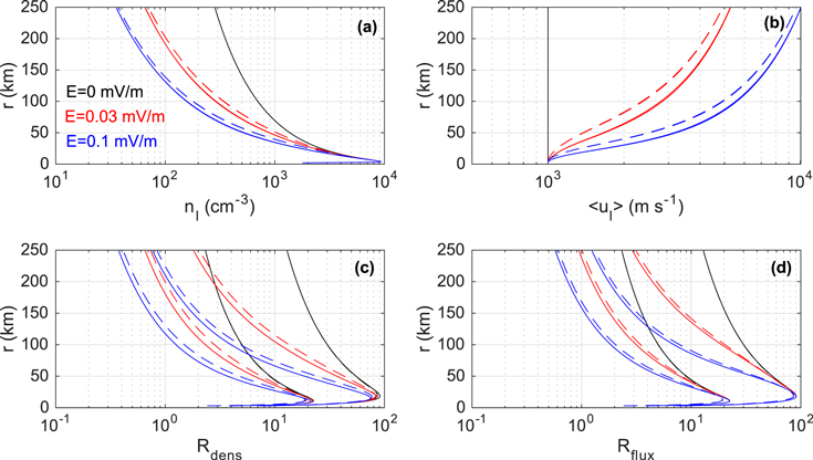
Figure 1. Shown vs. cometocentric distance are, as calculated from the TRAIN model, (a) ion number density, (b) mean ion flow speed, (c) H3O+/H2O+ number density ratio, and (d) H3O+/H2O+ flux ratio. The color indicates the constant electric field strength considered. For each considered field strength there are four lines representing results from models A, A*, B, and B*. Some of these lines are overlapping and are therefore difficult to distinguish from each other. Dashed lines overlapping in panels (a) and (b) represent results from B and B* models (in which elastic scattering is included). Solid lines overlapping in panels (a) and (b) represent results from A and A* models (in which elastic scattering is excluded). In panels (c) and (d) a given dashed line is close to a solid one of the same color. The pair of lines with the lower ratios are results from the A* and B* models, wherein the cross section for the proton-transfer reaction H2O+ + H2O → H3O+ + OH is decreased for Erel < 1.5 eV compared with the cases of models A and B. For these simulations the activity level was set to Q = 2 × 1027 s−1.
Download figure:
Standard image High-resolution image
Figure 2. Same as in Figure 1, but for an activity of Q = 2 × 1028 s−1. In addition, thick dot-dashed lines are results from model B runs with Q = 2 × 1029 s−1, resulting (for a given electric field strength) in enhanced values of nI (panel (a)), Rdens (panel (c)), and Rflux (panel (d)) and lower values of  (panel (b)).
Download figure:
Standard image High-resolution imageTable 3. Summary of Parameters Utilized in the Simulations Associated with the Results Displayed in Figures 1–4 of the Paper
| Par. | Description | Values Applied for Runs Associated with Figures |
|---|---|---|
| u | Neutral outflow velocity | 1 km s−1 (Figures 1–4) |
| uT | Minimal considered relative velocity | 0.5 km s−1 (Figures 1–4) |
| Q | Gas production rate | 2 × 1027 s−1 (Figures 1 and 3(a)), 2 × 1028 s−1 (Figures 2, 3(b), and 4) |
| ν | Ionization frequency | 4.5 × 10⁻⁷ s−1 (Figures 1–4), affects only nI. |
| E | Electric field | Constant (Figures 1–3), 1/r dependent for r > ren (Figure 4) |
| ren | Limit below which E is set to zero | 100 km (Figure 4), NaN in other figures |
| FXH+ | Fraction of ions of type XH+ at ren | 0.5 (Figure 4), NaN in other figures |
| kDR | Rate coeff. for dissociative recombination | 1 × 10⁻⁶ cm3 s−1 (Figure 4), NaN in other figures |
Note. NaN means that the parameter did not need to be considered in some simulations.
Download table as: ASCIITypeset image
Note that even for the simulations with Q = 2 × 1028 s−1 all calculated mean ion flow speeds at ∼200 km are markedly higher than the neutral flow speed u, set to 1 km s−1. The thick dashed lines in Figure 2 are results from model B runs with Q = 2 × 1029 s−1. As seen in panel (b), at this high activity level the mean ion flow remains close to u for the cometocentric distances considered. It is noted that we utilized Ci,1 = 1 also in this high-activity case. Attenuation of the impinging EUV light leads in reality to decreasing ionization frequencies toward the surface. However, if we were to account for this, we would get even lower mean ion speed predictions, due to reduced fluxes of ions that have experienced acceleration over longer distances.
5.1.2. Results from a Model Assuming Efficient Proton Transfer from H3O+ at Low Energies
As discussed in Section 3.2, the cross section for the proton transfer from H3O+ to H2O may have a steeper energy dependence than in relation (13). We test here the effect of using for this process a cross section given by Equation 10(b). As a reminder, Equation 10(b) is an extrapolation by Fleshman et al. (2012) of the experimental data by Lishawa et al. (1990) for the proton transfer from H2O+ to H2O, and now we use it also for the proton transfer from H3O+ to H2O, with the exception that for this change we use the cross sections of model A (neglecting elastic collisions and using Equation 10(b) for reaction 9(b) regardless of energy). Figure 3 shows mean ion flow speeds calculated from model runs with Q = 2 × 1027 s−1 (panel (a)) and Q = 2 × 1028 s−1 (panel (b)) with considerations of constant electric fields of 0.03 and 0.1 mV m−1. It is seen that at least for the higher activity considered, the modification of the cross-section set has a significant influence on the coupling, i.e., on the ability of the neutrals to keep the mean ion flow speed close to that of the neutrals. However, as hinted at in Section 3.1 and further discussed in Section 5.5, the A (and B) model is most likely overestimating the H2O+-to-H2O proton-transfer cross section at very low collision energies, so that when applying the same cross-section relation for the H3O+-to-H2O proton transfer, one would expect an overestimated coupling efficiency. There is a need for investigations, experimental or theoretical, of ion–neutral reactions at low relative kinetic energies.
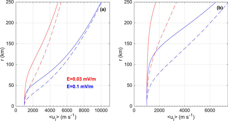
Figure 3. Shown vs. cometocentric distance are mean ion flow speeds as calculated from the TRAIN model for an activity of (a) Q = 2 × 1027 s−1 and (b) Q = 2 × 1028 s−1. Dashed lines are model A results, while solid lines are from simulations where the cross-section set is similar to model A with the exception of the cross section for the proton-transfer reaction H3O+(fast) + H2O → H2O + H3O+(slow), which, instead of being set equal to Equation (13), is set equal to Equation 10(b) regardless of relative kinetic energy.
Download figure:
Standard image High-resolution image5.2. Results from Model Runs with an Ambipolar Electric Field
A modification of the TRAIN model is to consider a limit where newly produced electrons switch from rapidly being thermalized to remaining hot. We set the border at ren, the electron–neutral decoupling distance. This limit, certainly more gradual in reality, is anticipated well within the zone where ions and neutrals remain coupled (Mandt et al. 2016), and so we may make some simplistic assumptions. We will assume that ions from below enter the shell starting at ren with velocity u. A fraction fXH+ of these are of the form XH+ (with X being some molecule, e.g., NH3, with higher proton affinity than H2O), and the complementary fraction is H3O+ ions. The reason for considering such molecules is because even if they prevail in low abundances, at the level of a percent or so, they can greatly influence the ion chemistry, as revealed by both modeling (e.g., Vigren & Galand 2013) and observations (Beth et al. 2017). For r > ren we assume that there is no additional production of XH+ ions, and that these species will not be lost chemically but will undergo acceleration along an ambipolar electric field. We make an initial assumption of a 1/r decay in the electron number density, which, combined with the constant electron temperature, sets up an ambipolar electric field of magnitude kBTe/qr accelerating ions radially outward (note that we neglect magnetic forces). In principle, we could also assume a more general 1/rγ decay of the electron number density, in which case the magnitude of the utilized ambipolar electric field (kBTe/qr) would need to be multiplied by γ. The outward direction of the ambipolar field may certainly be questioned in the near vicinity of ren, where we envision a sharp increase in Te. In the following, for the sake of simplicity we will assume that H2O molecules interrupt the acceleration of XH+ ions equally efficient as they do for H3O+ ions. This assumption affects also the formalism below. We do wish to stress, however, that experimental and/or theoretical studies into the mobility of XH+ ions in H2O gas when subjected to low electric fields are desirable.
In order to obtain estimates of key parameters, we may still use the TRAIN model but set r1 = ren instead of r1 = rC (an action that automatically adjusts, e.g., the Ni vector). In addition, we need to construct a new matrix Gi,j to account for ions originating from below ren, i.e., from what we refer to as the cold zone. We compute Gi,j from
with Gi,1 = 0 for all i > 1, with the product sign replaced by 1 in cases when i = j, and with G1,1 given by

The part within brackets is the ratio of Equation (12) of Gombosi (2015, pp. 169–88) and Equation (15) of the present paper. The parameter kDR is the effective recombination coefficient, which we take as constant within the cold zone (we will stick with a conservative value of 1 × 10⁻⁶ cm3 s−1). The bracketed part of Equation (22) is a measure of how much, relatively speaking, the electron density at (and within) ren is reduced when considering dissociative recombination in addition to radial transport (in the limit of  the bracketed expression equals 1). From Gj,j we compute gi,j according to

The key parameters discussed in Section 4 are now, within this modified approach, instead given by


and

We have used this modified approach for perihelion conditions with input parameters as specified in Table 3 and with resulting key parameters shown in Figure 4 and discussed in the next paragraph. The outgassing rate Q was set to match neutral number densities measured by COPS on 2015 August 1 near r = 200 km with the assumption of radial expansion and a constant outflow speed of u = 1 km s−1. We assume Te = 10 eV for r > ren = 100 km. The value set for ren is taken from Figure 5 of Mandt et al. (2016). Finally, we assume fXH+ = 0.5.

Figure 4. Same as in Figure 1, but for an activity of Q = 2 × 1028 s−1 and with the consideration of an ambipolar electric field E of magnitude U0/r for r > ren (U0 = 10 V) and 0 for r < ren = 100 km. The model type is indicated in the legend. The model "special" refers to a run with cross sections similar to model A, but with the exception of the cross section for the proton-transfer reaction H3O+(fast) + H2O → H2O + H3O+(slow), which, instead of being set equal to Equation (13), is set equal to Equation 10(b) regardless of relative kinetic energy. Note that model A and the "special" model, as anticipated, give identical Rflux values.
Download figure:
Standard image High-resolution imageThe outputs shown in Figure 4 are from the four model types A, A*, B, and B*, as well as from a modified version of model A with the cross section for Equation (12) given by relation 10(b) instead of Equation (13). To no surprise, A* predicts the highest mean ion flow speeds and consequently the lowest ion number densities. The ion density profiles are rather well described by 1/rγ relations for r > 110 km, and rough consistency may be achieved with small tuning of the assumed Te and the assumed electron density profile. We find that while the models give nI and  values at 200 km that are in reasonable agreement with limits constrained by LAP and MIP observations (typically ∼1000 cm−3 and a few kilometers per second, respectively), the H3O+/H2O+ number density and flux ratios are >5 and 7, respectively. With the extreme assumption of fXH+ = 1, the H3O+/H2O+ ratios at 200 km become >3.7 (number density) and >5.1 (flux). As a reminder, DFMS observations near perihelion reveal varying H3O+/H2O+ ratios, not seldomly in the vicinity of unity and even below (see Figure 7 of Fuselier et al. 2016). Speculatively this may reflect nonradial ion trajectories influenced by electromagnetic forces (see Section 6 for a brief discussion) and/or plasma instabilities, with energization of the ion population by plasma waves (see Sections 5.3.2 and 6).
5.3. Sensitivity of the Parameter

5.3.1. Temperature Effects
The parameter uT has for all model runs presented hitherto been set to 500 m s−1. As mentioned, uT may be said to represent a thermal component of the mean relative speed in collisions. In a gas of molecules characterized by a temperature T the mean relative speed in collisions between molecules of types 1 and 2 is (see, e.g., Equation (24.10) in Atkins & de Paula 2002)

with kB being Boltzmann's constant and μ1,2 the reduced mass of species 1 and 2 [m1m2/(m1 + m2)]. With H2O as the molecular type 1 and either H2O+ or H3O+ as the type 2, a mean relative velocity of 500 m s−1 corresponds to a temperature of ∼100 K. Considering a temperature as low as 20 K gives uT in the vicinity of ∼200 m s−1, while a higher temperature of 300 K gives uT ≈ 840 m s−1 (for theoretical estimates of kinetic temperatures in cometary comae, see, e.g., Tenishev et al. 2008). We have tested different values of uT for runs with cross sections according to model A but with the cross section for Equation (12) given by relation 10(b) instead of Equation (13). In these tests, performed for both Q = 2 × 1027 s−1 and Q = 2 × 1028 s−1, we used a constant electric field of either 0.03 mV m−1 or 0.1 mV m−1. The values of nI,  , and Rdens at r = 200 km for different utilized values of uT are summarized in Table 4. The parameter most influenced is the H3O+/H2O+ number density ratio, which drops markedly with increasing uT. The reason for the decreased number density ratio with increased uT is that the cross section for the proton-transfer reaction H2O+ + H2O H3O+ + OH decreases with increased relative velocity between the reactants. This effect is most notable when considering the A and B models, as in these models a rather steep energy dependence is applied for the proton-transfer reaction.
Table 4. Model Output at 200 km from Different Simulations as Described in Section 5.3.1
| Input | nI (cm−3) |
 (m s−1) (m s−1) |
Rdens | Input | nI (cm−3) |
 (m s−1) (m s−1) |
Rdens |
|---|---|---|---|---|---|---|---|
| Q1, E1, 200 | 111 | 3807 | 8.2 | Q2, E1, 200 | 3400 | 1042 | 588 |
| Q1, E1, 500 | 104 | 4100 | 3.1 | Q2, E1, 500 | 2861 | 1303 | 118 |
| Q1, E1, 840 | 100 | 4250 | 2.0 | Q2, E1, 840 | 2396 | 1640 | 45 |
| Q1, E2, 200 | 52 | 8548 | 1.9 | Q2, E2, 200 | 1727 | 3033 | 204 |
| Q1, E2, 500 | 51 | 8651 | 1.1 | Q2, E2, 500 | 1122 | 4443 | 32 |
| Q1, E2, 840 | 51 | 8699 | 0.8 | Q2, E2, 840 | 975 | 4976 | 15 |
Note. The columns labeled "Input" describe the difference between the models: Q1 is Q = 2 × 1027 s−1, Q2 is Q = 2 × 1028 s−1, E1 is E = 0.03 mV m−1, and E2 is E = 0.1 mV m−1. The number (200, 500, or 840) indicates the utilized value of uT in m s−1.
Download table as: ASCIITypeset image
5.3.2. Ion Motion due to Waves
We have so far worked with the assumption that the ions and the neutrals are characterized by similar temperatures when calculating uT. The motion of the ions may differ from neutral molecule motion for other reasons than the presence of electric fields or temperature considerations. In particular, low-frequency plasma waves and instabilities can provide ions with energy not directly accessible to the neutral gas. This need not be true for heating of the plasma by the wave, but the kinetic energy of the plasma motion inherent to the wave itself will for low-frequency waves reside mainly in the ions. The velocity average (with direction) in this motion is zero, but the mean energy and ion speed (magnitude of velocity) are not. We can let uT represent this mean speed in the wave motion of the ions just as well as random thermal ion motion, as an average over a wave period.
While much remains to be done on plasma waves at 67P, some results have been published. Richter et al. (2015) reported large-amplitude (ΔB/B ∼ 1) magnetic field fluctuations during pre-perihelion conditions, also seen in hybrid simulations by Koenders et al. (2015, 2016). Though the exact nature of these waves remains to be detailed, their very low frequency means that ion velocities associated with them are likely small, as is also the case for the mirror mode waves reported by Volwerk et al. (2016). Gunell et al. (2017) used data from LAP and the Ion Composition Analyzer (ICA; Nilsson et al. 2007) to suggest that ion acoustic waves may be unstable to the ion distributions seen at the comet. Karlsson et al. (2017) identified clear spectral peaks at the lower hybrid frequency in the LAP electric field measurements. As strong plasma density gradients are observed such waves could be generated through the drift lower hybrid wave instability at very fast growth rates, on the order of a wave period. In the terrestrial magnetotail, Norgren et al. (2012) observed such waves to acquire about 10% of the energy density available in the electron gas. This energy mostly resides in the ion motion. It may be noted that while Edberg et al. (2015) found the average plasma density during a Rosetta close flyby of the 67P nucleus in 2015 February to be consistent with a 1/r profile (as mentioned in Section 1), the data showed large variations (Δn/n ∼ 1) around the mean profile. There clearly are reasons to consider a situation in which a substantial fraction of the electron thermal energy is transferred to ion kinetic energy owing to ion motion in the wave.
In Table 5, we therefore display the sensitivity of uT to results from model runs similar to the ones described in Section 5.2 and Figure 4 (and its caption), but this time with an ambipolar electric field of magnitude E(r) = U0/r with U0 = 5 V, for r > ren = 100 km. Results are displayed for uT of 500 m s−1 (our default value) and 3000 m s−1, corresponding to ∼1 eV mean ion kinetic energy over a wave period. Again, among the listed parameters the H3O+/H2O+ number density ratio, Rdens, is the one most influenced, and the reduction becomes, of course, even more pronounced if considering even larger uT. An interesting by-product from these simulations is that the more energized the ion population one considers for r > ren, the more the H3O+/XH+ flux ratio will resemble the one at ren. This suggests that the effect of plasma waves on observables like the H3O+/H2O+ number density ratio and other ion number density ratios can be quite dramatic. However, if treating uT as a velocity vector perpendicular to the radial direction, we need to modify the regional absorption and survival probabilities (see Section 2 and Table 1) since when an ion travels a distance dr in the radial direction it will also travel a distance uT/uI,rad dr in the perpendicular direction, where uI,rad is the velocity of the ion in the radial direction (given by the vi,j or  arrays). The total distance traveled through the region will then amount to ds = (1 + (uT/uI,rad)2)1/2dr, and the exponents in the expressions for the regional absorption and survival probabilities (see Table 1) will need to be multiplied by ds/dr (note that ds is a variable). The influence of this modification is revealed by comparisons of data in Table 4 with data in Table 6, as well as by comparisons of data in Table 5 with data in Table 7. For uT = 500 m s−1 (the default value used when generating the data displayed in Figures 1–5) the effect is very small; the Rdens values, which are the most affected, increase only by ∼10% at Q = 2 × 1028 s−1, and less so for lower activity levels. However, as expected, the influence becomes more pronounced when considering higher uT. As seen in Table 7, the Rdens values at 200 km are still markedly decreased when increasing uT to 3 km s−1, but they fall below 3, and only marginally so, only in the A* model and when utilizing FXH+ = 1.

Figure 5. Ion energy distribution functions (dot-dashed lines) with the contribution from H2O+ (solid lines) and H3O+ (dashed lines) at r = 200 km. The functions were computed from model A runs with Q values of 2 × 1026 s−1 (black lines), 2 × 1027 s−1 (red lines), and 2 × 1028 s−1 (blue lines). A constant electric field of 0.03 mV m−1 was used for these simulations. In the high-activity case the H3O+ contribution to the total flux is very much dominating, and as such the blue dashed line is strongly overlapping with the blue dot-dashed line and is therefore not clearly visible.
Download figure:
Standard image High-resolution imageTable 5. Results from Model Runs at 200 km Similar to the Ones Described in the Caption of Figure 4 but with U0 Set to 5 V Instead of 10 V and with uT Set as Specified
| uT = 0.5 km s−1 | uT = 3 km s−1 | |||||
|---|---|---|---|---|---|---|
| Model Type | nI (103 cm−3) |
 (km s−1) (km s−1) |
Rdens | nI (103 cm−3) |
 (km s−1) (km s−1) |
Rdens |
| A | 1.43 | 2.53 | 49.5 (38.3) | 1.19 | 3.07 | 2.96 (2.17) |
| A* | 1.45 | 2.50 | 7.67 (5.79) | 1.19 | 3.05 | 1.91 (1.33) |
| B | 1.90 | 1.77 | 65.2 (49.3) | 1.43 | 2.46 | 3.42 (2.44) |
| B* | 1.91 | 1.76 | 10.2 (7.55) | 1.43 | 2.45 | 2.15 (1.45) |
| Special | 2.49 | 1.24 | 85.0 (63.7) | 1.30 | 2.77 | 3.29 (2.38) |
Note. Values within parentheses are for simulation runs wherein FXH+ was set to 1 instead of 0.5 (with our applied assumptions this affects only Rdens among the tabulated parameters).
Download table as: ASCIITypeset image
Table 6. Same as in Table 4 but with Consideration of Extended Pathways through Regions Following a Treatment of the Velocity uT as Perpendicular to the Radial Direction
| Input | nI (cm−3) |
 (m s−1) (m s−1) |
Rdens | Input | nI (cm−3) |
 (m s−1) (m s−1) |
Rdens |
|---|---|---|---|---|---|---|---|
| Q1, E1, 200 | 112 | 3798 | 8.4 | Q2, E1, 200 | 3404 | 1041 | 598 |
| Q1, E1, 500 | 104 | 4077 | 3.3 | Q2, E1, 500 | 2910 | 1274 | 132 |
| Q1, E1, 840 | 101 | 4210 | 2.2 | Q2, E1, 840 | 2502 | 1552 | 57 |
| Q1, E2, 200 | 52 | 8545 | 2.0 | Q2, E2, 200 | 1749 | 2995 | 211 |
| Q1, E2, 500 | 51 | 8642 | 1.1 | Q2, E2, 500 | 1148 | 4359 | 36 |
| Q1, E2, 840 | 51 | 8684 | 0.9 | Q2, E2, 840 | 1007 | 4847 | 18 |
Download table as: ASCIITypeset image
Table 7. Same as in Table 5 but with Consideration of Extended Pathways through Regions Following a Treatment of the Velocity uT as Perpendicular to the Radial Direction
| uT = 0.5 km s−1 | uT = 3 km s−1 | |||||
|---|---|---|---|---|---|---|
| Model Type | nI (103 cm−3) |
 (km s−1) (km s−1) |
Rdens | nI (103 cm−3) |
 (km s−1) (km s−1) |
Rdens |
| A | 1.45 | 2.51 | 55.0 (42.6) | 1.30 | 2.79 | 6.36 (4.82) |
| A* | 1.47 | 2.47 | 8.31 (6.28) | 1.31 | 2.77 | 3.82 (2.82) |
| B | 1.93 | 1.74 | 72.7 (55.0) | 1.64 | 2.10 | 7.98 (5.90) |
| B* | 1.94 | 1.73 | 11.2 (8.28) | 1.65 | 2.09 | 4.74 (3.41) |
| Special | 2.53 | 1.21 | 94.5 (71.1) | 1.50 | 2.37 | 7.37 (5.50) |
Download table as: ASCIITypeset image
5.4. Examples of Calculated Energy Distribution Functions
In Figure 5 we show IEDFs (dot-dashed lines) and the relative contribution to the fluxes of H2O+ (solid lines) and H3O+ (dashed lines) at r = 200 km calculated from model A with Q values of 2 × 1026 s−1 (black lines), 2 × 1027 s−1 (red lines), and 2 × 1028 s−1 (blue lines). For these runs we utilized constant electric fields of 0.03 mV m−1. As expected, the functions associated with lower Q are associated with higher ion energies and a higher relative contribution by H2O+ ions. Ion energy distributions are assessable from measurements by the ICA (Nilsson et al. 2007, 2015) and the Ion Electron Sensor (IES; Burch et al. 2007; Mandt et al. 2016). At low energies the measurements are affected by the spacecraft potential (typically ∼10–20 V negative; e.g., Odelstad et al. 2015; Eriksson et al. 2017), and so model–observation comparisons require detailed treatment, postponed for future studies.
5.5. Cross Sections at Low Collision Energy
We show here that if assuming Maxwellian energy distributions for the neutrals and the ions, the use of the cross-section relations 10(b) and 10(c) for reaction 9(b) at Erel < 1.5 eV gives rate coefficients at 300 K that differ somewhat from experimental values. For binary reactions, energy-dependent collision cross sections relate to temperature-dependent rate coefficients, k1,2(T), according to (e.g., Chapter 27.1 in Atkins & de Paula 2002)

where kB is Boltzmann's constant and μ1,2 is the reduced mass of the reactants. The experimentally determined value for Equation 9(b) at room temperature is 2.1 × 10⁻⁹ cm3 s−1 (Huntress & Pinizzotto 1973), while insertion of Equation 10(b) into Equation (28) gives a value of 7.4 × 10⁻⁹ cm3 s−1 at 300 K, higher than the experimental one by a factor of ∼3.5. Likewise, doing the same for Equation 10(c) results in 1.4 × 10⁻⁹ cm3 s−1, ∼34% lower than the experimental value. Obtaining the experimentally determined rate coefficient at 300 K and a temperature dependence (T/300)−0.5 as suggested in the UMIST database for astrochemistry (see Woodall et al. 2007), requires at low collision energies an energy-dependent cross section of approximately

where insertion of Erel in eV gives the cross section in 10−16 cm2. Such a function intersects with Equation 10(c) at Erel = 0.04 eV. Table 8 reveals the effect on predicted key parameters for model A* runs modified with the introduction of the cross-section relation (29) for Erel < 0.04 eV. It is noted that using Equation (28) for Erel < 0.04 and Equation 10(c) for higher Erel (up to 1.5 eV) as the cross section for the proton-transfer reaction 9(b) gives rate coefficients within 33% agreement with the formula 2.1 × 10⁻⁹ × (T/300)−0.5 up to temperatures of 1000 K. From Table 8 it is seen that five out of six considered models give roughly similar values of nI and  , but with marked variations in Rdens. The model labeled Aspecial is the one used for the data presented in Table 5 and yields, as seen in Table 6, the lowest values of
  . It is noted that in this model the reaction (12), i.e., the proton transfer from H3O+ to H2O, is given the cross-section relation 10(b) regardless of energy. Similar to what was noted above, applying such a cross-section relation at very low energies yields a 300 K rate coefficient significantly higher than derived experimentally by Smith et al. (1980). In summary, Equation 10(b) gives overestimated cross sections at very low energies, implying that models A and B will tend to yield overestimated H3O+/H2O+ number density ratios. Moreover, for a given field strength, models A and B, which in addition are modified to make H3O+ proton transfer to H2O equally efficient as the H2O+ proton transfer to H2O ("special models of A and B type"), will tend to overestimate the collisional coupling and therefore underestimate the mean ion drift speed.
Table 8. Model Outputs for r = 200 km for Simulations with Constant Electric Field of Magnitude 0.03 mV m−1 and for Q Values as Specified
| Q (s−1) | A* |

|
A |
|---|---|---|---|
| 2 × 1027 | 932; 4.57; 0.87 | 929; 4.59; 1.00 | 933; 4.60; 2.72 |
| 2 × 1028 | 1634; 2.60; 11.0 | 1630; 2.61; 16.1 | 1617; 2.62; 66.5 |
| 2 × 1029 | 31634; 1.13; 181 | 31632; 1.13; 315 | 31628; 1.13; 898 |
| Q (s−1) |

|

|
Aspecial |
| 2 × 1027 | 931; 4.58; 0.87 | 929; 4.59; 1.00 | 1036; 4.10; 3.12 |
| 2 × 1028 | 1630; 2.61; 10.9 | 1672; 2.55; 16.5 | 2861; 1.30; 118 |
| 2 × 1029 | 31588; 1.13; 181 | 33158; 1.07; 331 | 34865; 1.01; 990 |
Note. The u and uT parameters were set to 1 and 0.5 km s−1, respectively. An array such as "932; 4.57; 0.87" refers to the calculated values of nI (cm−3),  (km s−1), and Rdens, respectively. Model descriptions: models A and A* are as described in Table 2. Model
  is similar to A* but uses for reaction 9(b) the cross-section relation (29) for Erel < 0.04 eV. In models indexed by "special," reaction (12) is given the same cross-section relation as reaction 9(b) for the considered model case.
Download table as: ASCIITypeset image
5.6. Regarding Good Reproduction of Observations by Field-free Models at Low Activity

Vigren et al. (2016) reported an on average good agreement between modeled and observed electron number densities when Rosetta was at r ∼ 28 km and a heliocentric distance of ∼2.5 au in 2015 January 9–11. Their model was essentially Equation (14) with Q/u constrained from COPS measurements; so with u taken as ∼500 m s−1, Q ≈ 2 × 1026 s−1. The good agreement (see Figure 1 in Vigren et al. 2016) was argued to be indicative of the validity of central assumptions in the model, including the one of ions being coupled to the neutrals all the way to the spacecraft. The latter is not consistent with results from the TRAIN model, as discussed below.
When applying the TRAIN model to Q = 2 × 1026 s−1, a neutral outflow velocity of 500 m s−1, and weak electric fields, the neutrals are unable to interrupt acceleration of ions even well within cometocentric distances of 30 km. For example—with model A but with the use of an enhanced cross section for reaction (12) (see Section 5.1.2)—the use of a constant electric field of 0.03 mV m−1 (0.1 mV m−1) gives a mean ion flow speed at r = 28 km of ∼0.9 km s−1 (2.2 km s−1). For an ambipolar electric field of magnitude U0/r (with U0 = 5 V) for r > 20 km (for r > 10 km), the mean ion flow speed at r = 28 km becomes ∼3.2 km s−1 (4.2 km s−1). As electron temperatures on the order of 5–10 eV were measured by LAP in 2015 January, a strong ambipolar field could be expected, but from the observations presented in Vigren et al. (2016) it appears as if uI ≈ u.
The results from the TRAIN model indicate that such a low mean ion velocity cannot be due to frequent collisions with the neutrals, so a more probable explanation would be that the plasma was strongly influenced by the magnetic field environment and/or plasma waves, as discussed in Section 5.3.2 above. It should be noted that our treatment of the ambipolar electric field so far has been with an implicit assumption of either a very weak or absent magnetic field or one in the radial direction (i.e., parallel to the envisioned electric field). Given a moderately strong magnetic field at moderately high angle to the radial direction, electrons would be bound closer to the nucleus, effectively reducing the ambipolar electric field. This can to some extent be explored by hybrid simulations (e.g., Koenders et al. 2015), though due to their limited possibilities for modeling electrons, full particle-in-cell (PIC) simulations, not yet available, may be needed. A detailed investigation of magnetic field effects is beyond the scope of the present study.
6. Summary and Concluding Remarks
We have constructed a model that allows investigating radial ion acceleration in a cometary coma interrupted by collisions with H2O molecules. We have tested a variety of cross-section sets for ion–neutral interactions and considered cases of constant field strengths and ambipolar electric fields. With an extension the model can be updated to account for variations in the ionization frequency with cometocentric distance, to account for dissociative recombination (in a recursive fashion) and also to consider an extended set of both neutral and ionic species. The model is limited by its 1D nature and cannot account for nonradial movement of ions, which in reality may commence as a result of, e.g., magnetic forces, electric fields in nonradial directions, and angle scattering following ion–neutral interactions. With our utilized cross-section set the local mean free paths for water group ions as calculated for conditions at the Rosetta location in early 2015 August are smaller than or on the same order as their gyroradii given a magnetic field of 10–20 nT perpendicular to the radial direction.
In early 2015 August, just prior to perihelion, Rosetta resided at cometocentric distances of 200–300 km, and from COPS measurements (see Beth et al. 2017) of neutral number densities an activity parameter Q ≈ 1 to a few times 1028 s−1 can be inferred, assuming a neutral outflow speed of 1 km s−1. Whether the ions near the spacecraft location at this time period were collisionally coupled or not is currently under investigation by analysis of LAP and MIP data, with preliminary results giving upper limits (see Section 1) of the mean ion drift speeds in the range of 2–8 km s−1, markedly higher than the expected neutral outflow velocity.
From our model runs we may conclude that by r = 200 km ions are expected to be collisionally decoupled for an activity of Q = 2 × 1027 s−1 but coupled for an activity of Q = 2 × 1029 s−1. By "coupled" we mean here that the mean ion drift speed is roughly similar to the neutral counterpart. For an activity level of Q = 2 × 1028 s−1 it is more difficult from our model runs to state firmly whether or not the ions are expected to be coupled to the neutrals or not by r = 200 km. This uncertainty is due to uncertainties on the energy dependence of the cross section for some processes and in part also due to uncertainties in the parameter uT. While models A, A*, B, and B* (see Table 2) all show an inability of the neutrals to hamper ion acceleration in the presence of weak electric fields (see Figure 2(b)), a model of type A, but with enhanced cross sections for the proton transfer from H3O+ to H2O (similar to the cross section for the proton transfer from H2O+ to H2O), keeps the mean ion flow speed not drastically above the neutral speed all the way out to 200 km (see Figure 3). However, as pointed out in Section 5.5, it is very probable that the A (and B) model is associated with too high H2O+-to-H2O proton-transfer cross sections at very low collision energies, and so when using these cross sections also for H3O+ collisions with H2O, the efficiency of that interaction will also be overestimated. To resolve questions, there is a need for detailed studies, experimental and theoretical, particularly into the proton-transfer reaction H3O+ + H2O → H2O + H3O+ at low relative kinetic energies. In these reactions we envision fast impinging hydronium ions to be replaced by slow ones with about the same speed as the neutrals. The latter assumption can be questioned; as discussed in Section 3.3, the experiment by Smith et al. (1980) revealed that the interaction proceeds via a long-lived intermediate adduct ion, meaning that the emanating ion need not be much slower than the impinging one.
For Q = 2 × 1028 s−1 the calculated H3O+/H2O+ number density ratios and flux ratios at 200 km are strongly dependent on the cross section for the proton transfer from H2O+ to H2O. However, regardless of model type and electric field considered in this paper, the ratios are >5 (number density ratio) and >7 (flux ratio). As such, the H3O+/H2O+ ratios derived from DFMS measurements and presented in Figure 7 of Fuselier et al. (2016) are often so low that they are difficult to explain by cold ion motion radially outward. An H3O+/H2O+ number density ratio of ∼1 at r = 200 km is reached in a model A* run for Q = 2 × 1028 s−1 when applying a constant electric field of 1 mV m−1. However, the calculated ion number density and ion flow speed at 200 km then become ∼200 cm−3 and 25 km s−1, respectively. Such estimates strongly conflict with limits constrained currently from LAP and MIP measurements.
Low measured H3O+/H2O+ ratios may reflect ion trajectories at the considered time and a location not well described as radial, but strongly influenced by electromagnetic forces (see, e.g., the hybrid simulations by Koenders et al. 2015). With source regions far off from the radial direction, chances increase that H2O+ ions escape interactions prior to reaching the spacecraft. Another explanation could be that the energy of the free electrons is used partly to energize the ion population via plasma waves, for example, lower hybrid waves (Karlsson et al. 2017). The ion motion in such waves increases the relative speed in ion–neutral collisions, thereby reducing the coupling efficiency by collisions (see Section 5.3.2). Real heating of the ions is not needed, as the regular collective motion in a plasma wave would have a similar effect. Finally, the good reproduction of observed electron number densities by field-free models at low activity (see Section 5.6) raises concerns, as we have here verified that the coma was not dense enough to enable collisional interruption of ion acceleration along weak electric fields. It appears as if the energy of the free electrons cannot have gone significantly into radial acceleration of the ions. Plasma waves are an obvious degree of freedom that this energy may end up in.
We are grateful for funding from the Swedish National Space Board, contract No. 166/14.