


ABSTRACT
The G7 IIIa single-lined spectroscopic binary, β Her, is studied with high-resolution, high-signal-to-noise spectra taken over 10 seasons from 23MR2000 to 10MY2009. Absolute radial velocities, corrected for convective blueshifts, are determined and new orbital parameters are derived. Line-depth ratios are used to measure temperature variation ∼2 K. A Fourier analysis is done for the line broadening, yielding a projected rotation velocity of 3.27 ± 0.20 km s−1 and a radial–tangential macroturbulence dispersion of 6.43 ± 0.08 km s−1. The "C" shaped bisector of Fe i λ6253 has its blue-most point at a relative flux level of 0.52, consistent with what is expected from β Her's absolute magnitude. The third-signature plot indicates granulation velocities 20% larger than the Sun's. Mapping the λ6253 line bisector onto the third-signature curve results in a flux deficit of 12.6 ± 1.0% that can be interpreted as arising from a temperature difference between granules and inter-granular lanes of 132 K. The flux deficit peaks near 5.5 km s−1 from the line center, suggesting the velocity difference between granules and lanes is ∼20% larger than that found for recently analyzed K giants.
Export citation and abstract BibTeX RIS
1. HISTORY
Although β Her (HR 6148, HD 148856, HIP 80816) is a well-known single-lined spectroscopic binary and is bright (V = 2.77), it has not attracted much attention, aside from radial velocity measurements and surveys. Campbell (1900) discovered the variation in radial velocity and presumed the star to be a binary. Nearly a decade later Plummer (1908) published the first orbit based on 34 exposures taken between 13JN1898 and 25FE1908. His orbit was quite respectable and is discussed below in Section 3. A few additional radial velocities were contributed in the early 1900s, but the next orbital solution came a century later based on 127 high-quality velocities measured by Eaton & Williamson (2007). Additional work by Massarotti et al. (2008) contributed 10 new observations and additional orbital solutions. In Section 3 below, 37 new values of still higher accuracy are given on an absolute scale, i.e., with convective blueshifts removed, and new orbital parameters are determined. The secondary component is much fainter than the primary and has not been seen.
Most commonly β Her is classified as G8 III, but Keenan & McNeil (1989) place it at G7 IIIa in their refined list. The slightly earlier type is supported by the star's  color index of 0.93 (Ducati 2002) compared to the more typical value of 0.96 for the G8 III class. The intrinsic
  might even be slightly smaller by ∼0.02 if the interstellar extinction calculated by Maldonado et al. (2013) is applied. Combining the Hipparcos parallax (van Leeuwen 2007) of 23.44 ± 0.58 mas (42.7± 1.1 pc) with the apparent visual magnitude,
  (or −0.43 if the extinction of Maldonado et al. is included). This places the star close to a full magnitude above the mean value for class III in agreement with the IIIa classification. As we shall see in Section 6, the λ6253 line bisector shape is also in accord with the higher luminosity class.
A few values of effective temperature, surface gravity, and metallicity have been published. McWilliam (1990) found 4920 K, Allende Prieto & Lambert (1999) determined 5012 K, Luck & Heiter (2007) list 5103 K, Massarotti et al. (2008) give 4887 ± 5 K, and Soubiran et al. (2008) obtain 4967 K. Maldonado et al. (2013) give a spectroscopically determined temperature of 5038 K and a value from evolutionary tracks of 4973 K. Gray & Brown (2001), using line-depth ratios (LDRs), found 4987 and 4994 K from two color-index calibrations based on the temperature scale of Taylor (1999). Taylor's value for β Her was 4927 K. The polynomial Equation (14.17) in Gray (2005b), with B-V = 0.93, yields 5034 K, the polynomial by Gratton et al. (1996) gives 4987 K, and the tabulation by Flower (1996) has 4984 K. The effective temperature is used below to calculate the thermal component of the line broadening (Section 5) and only an approximate value is needed. I adopt 4990 K.
In a similar vein, published surface gravity (log g values) are: McWilliam (1990) 2.62, Allende Prieto & Lambert (1999) 2.47, Luck & Heiter (2007) 2.85, Massarotti et al. (2008) 2.5, Maldonado et al. (2013) 2.54 spectroscopically, 2.53 from evolutionary tracks. While the model photospheres computed in Section 5 require a log g value, the results are essentially independent of the value used, and log g = 2.6 was chosen for the calculations.
Values of metallicity, [Fe/H], from the literature include McWilliam (1990) −0.27, Taylor (1999) −0.083 ± 0.054, Luck & Heiter (2007) −0.03, and Maldonado et al. (2013) −0.08. An early study by Griffin (1969) found approximately solar metallicity. I use −0.08 in the models below.
An estimate of the angular diameter based on surface brightness of 4.1 mas was found by Wesselink et al. (1972), which in linear measure is 19 solar radii, assuming the updated parallax of 23.44 mas. Blackwell & Lynas-Gray (1994) computed an angular diameter of 3.48 ± 0.14 mas from the integrated energy distribution, or  . Allende Prieto & Lambert (1999) use evolutionary models to estimate a radius of 16.9
  and mass of 3.07
  . Using similar techniques, these values were essentially confirmed by Pizzolato et al. (2000), Pasquini et al. (2000), Luck & Heiter (2007), Massarotti et al. (2008), and Maldonado et al. (2013), although a somewhat smaller radius of 15.2
  was found by this last group. Direct interferometer observations by Mozurkewich et al. (2003, see also Nordgren et al. 2001) gave an angular diameter of 3.46 ± 0.04 mas or a radius of 15.9 ± 0.4
  .
.
Determinations of projected rotation rates for β Her are sparse. I did an early Fourier analysis (Gray 1982) that gave v sin i = 3.4 ± 0.8 km s−1 and a radial–tangential macroturbulence dispersion  km s−1. Fekel (1997) used half widths of a few lines to find v sin i = 3.0 km s−1, but this value is not independent of the 1982 value since he used the Fourier results to calibrate his measurements. He made an approximate correction for the broadening of macroturbulence. De Medeiros & Mayor (1999) used the width of cross-correlation curves from their CORAVEL instrument to estimate v sin i = 4.8 ± 1.0 km s−1 after making an empirical correction for macroturbulence. With a similar correlation technique, Massarotti et al. (2008) found a value of 2.8 km s−1, but they too corrected for an assumed macroturbulence dispersion of 6.3 km s−1. In their rotation catalog, Głȩbocki & Gnaciński (2005) also list Pasquini et al. (2000) and De Medeiros et al. (2002), but these are replications of the De Medeiros & Mayor (1999) value.
Granulation characteristics of stars are hard to pin down because of our inability to resolve stellar surfaces. Almost nothing is known about the granulation characteristics of β Her. As mentioned in the previous paragraph, a macroturbulence dispersion (the first signature of granulation) of 4.8 km  was determined a third of a century ago. The new value found below (Section 5) is much better determined and is significantly larger. Bisector shapes, the second signature of granulation, have not been published for this star. The bisector of the λ6253 line is documented below in Section 6 and used to study granulation contrast in Section 8. The third granulation signature, namely the larger blueshifts shown by weaker lines, is used in Section 7 to explore the convective velocity scale and to establish the star's radial velocity free of the systematic errors arising from the convective blueshifts.
Like α Ser (Gray 2016b), β Her has low chromospheric emission based on the Mt. Wilson S index of 0.11 according to Young et al. (1989) and Duncan et al. (1991); see also Pérez Martínez et al. (2014). Values this low actually lie at the lower boundary of all measured values and that implies minimal magnetic activity. A different picture is indicated by the HK flux measurements of Pasquini et al. (2000). The HK flux they found places β Her in the middle of the pack, not at a lower boundary. The Mg II HK lines show moderate emission (Simon et al. 1982), but according to Cassatella et al. (2001, see also Scoville & Mena-Werth 1998) has a 'Wilson–Bappu' width more characteristic of stars ∼3 mag brighter than it actually is. Vaughan & Zirin (1969) found no He I λ10830 line in their survey. On the other hand, the star shows coronal emission lines, particularly C IV, normal X-ray emission, and lies on the hot side of the coronal boundary in the HR diagram (Linsky & Haisch 1979; Simon et al. 1982; Pizzolato et al. 2000). No infrared variation was seen in the survey done by Price et al. (2010).
This is the fourth paper of a series in which detailed line-profile analysis is done for stars using high-resolution, high-signal-to-noise data. The analysis of β Gem (Gray 2014) is Paper 1, ε Cyg (Gray 2015, 2016a) is Paper 2, and α Ser (Gray 2016b) is Paper 3.
2. SPECTROSCOPIC OBSERVATIONS
Between 23MR2000 and 10MY2009, 46 exposures of β Her were recorded at the Elginfield Observatory using the coud spectrograph (Gray 1986, 2005b). The first 10 of these were taken prior to the installation of radial-velocity capabilities (Gray & Brown 2006). Based on continuum photon count, the signal-to-noise ratios (S/Ns) ranged from 196 to 543 with a mean of 352 and a median of 343. Figure 1 shows the full field recorded by the 200 × 4096 pixel CCD. The nominal resolving power is  . Additional details concerning the spectrograph, general reduction procedures, and absolute wavelength calibration are available in Papers 1–3.
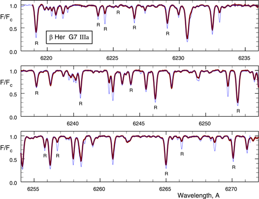
Figure 1. The ordinate, F/Fc, is flux normalized by the continuum value. Thicker line: β Her, thinner line: ε Cyg, K0 III (Paper 2). The 16 lines used in the rotation/macroturbulence analysis are tagged with an R.
Download figure:
Standard image High-resolution imageThe 16 lines labeled with an R in Figure 1 are used in the rotation/macroturbulence analysis (Section 5 below). The spectral lines of ε Cyg, also shown in Figure 1 for comparison, are generally stronger than those of β Her, as one expects for a cooler star. There are notable exceptions like the Si i lines are 6237 and 6238 Å. The lines of β Her are also wider, but that is hard to see in the figure.
3. RADIAL VELOCITY AND ORBITAL SOLUTION
The radial velocities of 38 lines in each exposure were measured by fitting vertically oriented parabolae to the cores. Rest wavelengths were taken from Gray & Pugh (2012) but ultimately are based on the iron line measurements of Nave et al. (1994). Because the wavelength calibration of the spectra is based on water vapor lines formed within the coude spectrograph and there is only one such line toward the long-wavelength side of the exposures, only lines below 6260 A were used for velocity work. Empirical weights were used when combining the velocities from the 38 lines into an exposure mean. These weights were computed based on the observed scatter of each line across the 36 exposures relative to the unweighted exposure mean. (Direct absolute scatter, which would normally be used, would include the orbital motion.) The scatter varies from line to line because (1) the wavelength calibration is best determined near the center of the exposures and (2) the slope of the sides of the weaker profiles is smaller, translating photometric error into larger velocity error compared to stronger lines. Finally the velocities were adjusted to an absolute scale using the mean third-signature plot discussed below in Section 7. The velocities for 36 dates are compiled in Table 1.
Table 1.
β Her Absolute Radial Velocities (m  )
)
| Year | JD-2450000 | Velocity (m s−1) |
|---|---|---|
| 2001.5320 | 2102.697 | −18459 ± 53 |
| 2001.5373 | 2104.617 | −19545 ± 88 |
| 2001.5947 | 2125.566 | −26644 ± 75 |
| 2001.6221 | 2135.562 | −28353 ± 57 |
| 2002.2504 | 2364.891 | −27962 ± 162 |
| 2002.4009 | 2419.824 | −22733 ± 200 |
| 2002.4719 | 2445.737 | −17946 ± 72 |
| 2002.6115 | 2496.713 | −7979 ± 130 |
| 2003.5375 | 2834.687 | −22400 ± 77 |
| 2003.7179 | 2900.540 | −6239 ± 55 |
| 2004.4133 | 3154.776 | −29412 ± 119 |
| 2004.4542 | 3169.727 | −29162 ± 75 |
| 2004.4814 | 3179.675 | −28311 ± 72 |
| 2004.5305 | 3197.648 | −27151 ± 68 |
| 2005.2887 | 3474.877 | −31837 ± 77 |
| 2005.3488 | 3496.824 | −31617 ± 53 |
| 2005.4800 | 3544.710 | −30317 ± 189 |
| 2005.4992 | 3551.701 | −29995 ± 121 |
| 2005.5401 | 3566.638 | −29428 ± 83 |
| 2006.2229 | 3815.843 | −31281 ± 132 |
| 2006.3542 | 3863.791 | −31984 ± 55 |
| 2006.4500 | 3898.733 | −31995 ± 26 |
| 2006.4554 | 3900.720 | −32013 ± 70 |
| 2006.5210 | 3924.664 | −31088 ± 61 |
| 2007.3079 | 4211.881 | −30508 ± 72 |
| 2007.4828 | 4275.716 | −32192 ± 79 |
| 2007.5702 | 4307.617 | −31813 ± 110 |
| 2007.5756 | 4309.603 | −31704 ± 123 |
| 2008.3969 | 4609.761 | −29299 ± 61 |
| 2008.4159 | 4616.722 | −30048 ± 50 |
| 2008.4787 | 4639.713 | −31736 ± 50 |
| 2008.5278 | 4657.666 | −31694 ± 114 |
| 2008.5850 | 4678.613 | −32022 ± 127 |
| 2009.2286 | 4913.938 | −17472 ± 130 |
| 2009.2640 | 4926.854 | −13569 ± 24 |
| 2009.3626 | 4962.860 | −8509 ± 156 |
Download table as: ASCIITypeset image
Owing to the sparseness of the observations compared to the orbital period (discussed below), determining the errors on the velocities is challenging. The rms scatter of individual spectral line velocities minus their exposure mean is ∼120 m s−1. With 38 lines entering the exposure mean, one might expect the average exposure mean to be uncertain by ∼120/381/2 ∼ 20 m s−1. But this must be too low because systematic errors affecting all the lines in an exposure are not included. To compare with previous investigations, the S/Ns of the β Her data are only slightly less that those for β Gem (Paper 1), ε Cyg (Paper 2), and α Ser (Paper 3), where typical rms scatter was found to be ∼75, 85, and 90 m s−1 respectively. All these values include other variations such as non-radial oscillations (McMillan et al. 1992, Figure 12 in Paper 2) that can span ∼100 m s−1 and contribute ∼30 m s−1 to the rms number. Assuming similar errors occur for all three stars, the average velocity error for β Her should be less than 100 m s−1. Using a conservative estimate of 90 m s−1 as the average error across 36 exposures, the errors in Table 1 are made proportional to the observed scatter among the lines of each exposure.
Although several previous publications give radial velocity measurements of β Her, of particular importance are the century-old observations of Plummer (1908) because, when combined with the results in Table 1, ∼93 period cycles have been traversed, making for a precise determination of the period, namely 1.1254 ± 0.0001 years (411.04 ± 0.04 days). Armed with the period, the various measurements from the literature are phased with those in Table 1 as shown in Figure 2. The observations in Table 1 have good phase coverage as do those of Plummer (1908, 34 observations) and Eaton & Williamson (2007, 127 observations). (Thanks to J. Eaton who was kind enough to send me his unpublished velocities to include in Figure 2.) Other investigations contribute lesser numbers. Errors on early photographic determinations are estimated by Griffin (1994) to be ∼1–2 km s−1, consistent with the ∼2 km s−1 errors given by Kustner (1908, six observations). As implied by Plummer, his observations have an rms scatter of ∼0.9 km s−1, while Massarotti et al. (2008, 10 observations) indicate their values are good to ∼0.2 km s−1. Additional contributions were made by Lunt (1918, three observations) and Beavers & Eiter (1986, one observation). The velocities of each of these data sets were shifted to correspond to the absolute zero point of the observations in Table 1. As seen in Figure 2, observations from these various sources are consistent within the errors of measurement and the curve is well determined.
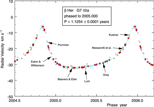
Figure 2. Velocities from various sources are phased to the results from Table 1. The agreement among the data sets is so good that points often obscure each other.
Download figure:
Standard image High-resolution imageRefined orbital parameters were then determined using the 1.1254 year period and the velocities in Table 1. Figure 3 shows the computed orbital velocities compared to the observations. The residuals are shown around the systemic velocity (γ) and have an rms scatter of 0.167 km s−1. The orbital parameters are summarized in Table 2. Errors were estimated by varying one orbital parameter at a time and monitoring the change in residuals. There is relatively little crosstalk among the variables. An error in semi-amplitude (K) produces systematic offsets in the sections above and below the systemic velocity. The eccentricity (e) is constrained mainly by the width of the upward peak. Variation in the longitude of periastron (ω) are most strongly seen as changes in the slope of the broad minimum. The time of periastron passage (T0) is constrained by the sharpness of the rise peak. Previous orbit determinations by Massarotti et al. (2008), Eaton & Williamson (2007), and by Plummer (1908) are also listed in Table 2 for comparison. In the main, my new orbital parameters are in excellent agreement with the results of Eaton & Williamson.
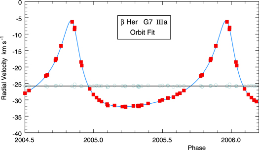
Figure 3. Computed orbital velocity (line) compared to the observations from Table 1 (squares). The residuals, observed minus computed velocities, are shown around the systemic velocity (circles). Their rms scatter is 0.167 km  .
.
Download figure:
Standard image High-resolution imageTable 2. Orbital Parameters of β Her
| Element | Gray (This Paper) | Massarotti et al. (2008)a | Eaton & Williamson (2007) | Plummer (1908)b |
|---|---|---|---|---|
| P (years) | 1.1254 ± 0.0001 | 1.1310 ± 0.0140 | 1.1241 (Plummer)c | 1.1241 (±0.004) |
| e | 0.5613 ± 0.0010 | 0.586 ± 0.036 | 0.561 ± 0.001 | 0.550 (±0.005) |
| K (km s−1) | 13.05 ± 0.05 | 12.32 ± 0.44 | 13.11 ± 0.03 | 12.782 (±0.14) |
| ω (deg) | 21.9 ± 0.05 | 19.7 ± 4.6 | 23.0 ± 0.3 | 24.6 (± 2.3) |
T (date)d (date)d
|
2004.8514 ± 0.0001 JD 3315.12 ± 0.04 | 2004.840 ± 0.026 JD 3310.9 ± 9.3 | 2004.8527 ± 0.0003 JD 3315.58 ± 0.12 | 2004.855 (±0.001) JD 3316.05 (±0.3) |
| γ (km s−1) | −25.775 ± 0.030e | −25.77 ± 0.54f | −26.13 ± 0.02 | −25.52 (±1.00) |
Notes.
aMassarotti et al. (2008) give three orbital solutions. The one listed here is for their observations alone. When they add the values from Plummer (1908), P = 1.1242 ± 0.0021, e = 0.545 ± 0.015, K = 12.84 ± 0.29. If they include all published values, P = 1.1254 ± 0.0001, e = 0.546 ± 0.011, K = 13.090 ± 0.230, and the other elements are not given. bValues in parentheses are my estimates based on the solution attributed to H.M. Reese in Plummer (1908). cPlummer's period was used. dYear followed by Julian Day less 2,450,000 days. eThe precision of the orbit fit to the observations is ±0.03 km s−1, but the calibration error on the absolute velocities themselves is ∼0.05 km s−1. fAn offset of 0.14 km s−1 was added their Table 10 value in accordance with the statement on page 216 of their paper.Download table as: ASCIITypeset image
Using the period, eccentricity, position of periastron, and epoch of periastron passage from Plummer (1908), Jancart et al. (2005) probed the Hipparcos data for an astrometric orbit. They found an angular semimajor axis of 11.37 ± 0.51 mas, the orbital inclination i = 53 80 ± 130, and the longitude of the ascending node Ω = 3419 ± 38. With the parallax noted above, the semimajor axis for the primary or A component is aA = 0.485 ± 0 0.025 au. Alternatively, using the definition of K,

and the spectroscopic orbital values for K, P, and e, along with the astrometric inclination, results in a semimajor axis of aA = 0.504 ± 0.034 au, where the error is overwhelmingly dominated by the uncertainty in the inclination.
Since the secondary is not visible, we can reasonably presume it is a dwarf cooler than ∼G2 or a white dwarf. Either way, its mass is then ∼1 solar mass. As a G7 giant, the primary's mass is likely to be no smaller than 2 and no larger than 3.5 solar masses, or the sum of the masses lies between ∼2 and 4.5 solar masses. Invoking Kepler's third law implies a mass ratio between ∼1.7 and 2.6 and a full semimajor axis, a = aA + aB, between ∼1.4 and 1.8 au.
It is worth re-iterating that the residuals around the orbital solution have an rms scatter ∼0.167 km s−1 or ∼167 m s−1, a value approximately twice as high as would be expected from the estimated velocity errors. This is consistent with many other indications of low-level velocity variations shown by evolved stars. Furthermore, the distribution of the residuals is asymmetric in the same sense as the one for α Hya that was attributed to convective cells (Gray 2013).
4. LDRS: TEMPERATURE VARIATIONS
The ratios of the central depths of temperature-sensitive to temperature-stable lines is a powerful index of temperature differences or variations (Gray & Johanson 1991; Gray & Brown 2001, and other references in Paper 2). Here 10 line-depth ratios (LDRs) are employed to sense any temperature variation in β Her. Most of these ratios are the same as in Table 1 of Paper 1. Several combinations are readily seen in Figure 1. Each LDR was converted to temperature variation, as done in Papers 2 and 3, by first subtracting off the mean over the 10 seasons of observation and then dividing by the temperature sensitivity. The observational noise is automatically scaled into temperature units by application of the sensitivity factors. An exposure-mean of these temperature differences was formed using weights inversely proportional to this temperature noise. The open circles in Figure 4 show the exposure-mean LDR-temperature values. Season means, i.e., averages of the exposure-mean values within each observing season, were computed using weights proportional to the continuum photon count in the exposures. The season means are shown as squares in Figure 4. The average error on the season means is 0.7 K, whereas the scatter of the season means themselves is 1.2 K, suggesting some real variability.

Figure 4. Circles: exposure-mean temperatures from LDRs shown as a function of time. Squares: season means. Triangles: means of Hipparcos photometry from 1990–93 arbitrarily shifted in time and magnitude, but with the 22 mmag span set to match the ±10 K ΔT ordinate interval.
Download figure:
Standard image High-resolution imageExploration of the Hipparcos photometry, taken between early 1990 and early 1993, shows a clear systematic brightening. Since the errors on individual measurements are quite large, I binned the data to better see the variation. Model photosphere computations show that a one degree change in stellar temperature corresponds to 1.1 mmag at the 5600 Å wavelength of the Hipparcos photometry (Bessell 2000). The bin-mean magnitudes are shown as triangles in Figure 4. The timescale is the same as for the LDR plot, but arbitrarily shifted into the time range of my observations. The magnitude scale was adjusted so that 1.1 mmag corresponds to 1.0 K. No direct comparison can be made since the two sets of data do not overlap in real time, but what we can see is that the photometric variations, if interpreted as arising from temperature variation, show an amplitude and timescale that is similar to the LDR result.
Similar and larger variations in temperature were found for ε Cyg (Paper 2), but no variation was detected for β Gem (Paper 1) or α Ser (Paper 3).
The several-year timescale of the variability in Figure 4 rules out rotational modulation, which has periods of ≲ 1 year (see the end of Section 5) and non-radial oscillations, which have periods ∼ hours (Huber et al. 2011). Given the modest radius ∼16 R⊙ (Section 1), large convection cells (Gray 2013) seem unlikely. Magnetic cycles remain as the most probable cause, although little is known about magnetic cycles in giants (e.g., Baliunas et al. 1998). Solanki et al. (2013) discuss similar variations for the Sun.
5. ANALYSIS OF LINE BROADENING: ROTATION AND MACROTURBULENCE
The dominant components of line broadening in these spectra are the Doppler shifts of rotation and macroturbulence. The broadening and shape of the line profiles are investigated by Fourier analysis to extract two parameters, the projected rotation rate, v sin i, and the radial–tangential macroturbulence velocity dispersion,  .
.
In cool stars like β Her, most of the lines are too blended to be useful. The 16 lines labeled with an R in Figure 1 were selected for analysis. The profiles were extracted from each of 43 exposures (three exposures being omitted owing to various photometric flaws) and averaged using weights proportional to the continuum S/N. Based on the combined photon count, the S/N should be ∼2400. This is so large that other sources of error and variation will come into play, such as imperfect focus of the spectrograph and occasional undetected cosmic ray hits to the CCD. In any case, statistical errors are small compared to the uncertainties introduced by line blending. Obvious blends were corrected manually by matching the wavelength-reversed profile with itself, assuming a symmetric profile. In fact, the intrinsic profiles are not perfectly symmetric, as discussed below, but the asymmetry is not only small compared to the distortions of the line blending, but blend corrections are made only to line wings, where the asymmetry has virtually no affect.
The Fourier transforms of the 16 line profiles are shown in Figure 5. The thermal components of the profiles were computed using a model photosphere with  K, log g = 2.6, [Fe/H] = −0.08, and a temperature distribution based on Ruland et al. (1980); see also Paper 1. Isotropic microturbulence is incorporated into the thermal component in the usual manner (e.g., Gray 2005b, Equation (11.45)). For the 12 weakest lines, microturbulence dispersion, ξ, has little influence on the transforms and a value of ∼0.7 km s−1 was used. For the four strongest lines the first sidelobe could be used to determine ξ. Generally ξ is larger for stronger lines, the largest value being for λ6253 with ξ = 1.6 km s−1. Transforms of the thermal profiles are the middle set of curves in Figure 5. They are divided into the transforms of the observed profiles to yield the residual transforms shown as the top set of curves in Figure 5. In principle, all residual transforms should be identical. The scatter of these curves is a measure of the uncertainty and is used to compute the errors shown in Figure 6. Careful inspection of the figure reveals four spikes, two smaller and two larger, between abscissa values of −1.0 and −0.8. They are artifacts arising from the division of very tiny values in the line transform by very tiny values in the thermal-profile transform at the first zeros of the four strongest lines. These are ignored in the analysis that follows. Only amplified noise is seen at frequencies higher than ∼−0.8 dex.
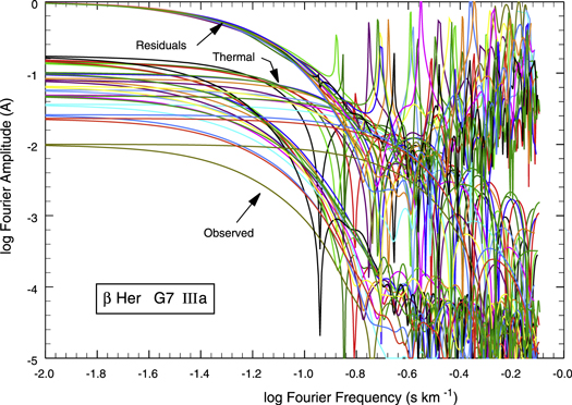
Figure 5. Fourier transforms for the 16 lines used in the analysis. The lowest set is for the observed profiles, the middle set for the computed thermal profiles, and the uppermost set shows the residual transforms. The residual transforms are consistent and can be followed up to log frequency ∼−0.8, beyond which amplified noise takes over. Noise spikes between −0.8 and −1.0 correspond to the first zeros in the transforms of the four strongest lines, where near-zero values are divided by near-zero values.
Download figure:
Standard image High-resolution image
Figure 6. The lowest symbols (+) show the mean of the residual transforms of β Her (from Figure 5). The circles with error bars are the same data after division by the transform of the instrumental profile. Error bars are the standard deviations for the mean residual transform. They are smaller than the symbols at low frequencies. The solid line is the model with v sin i = 3.27 and  km s−1. Two other models (dashed lines) are shown to indicate the sensitivity. They have v sin i = 2.0,
  and v sin i = 4.0,
  .
.
Download figure:
Standard image High-resolution imageA weighted average of the residual transforms is shown by the small crosses in Figure 6. The weights were set by the S/N of the transforms of the observed line profiles combined with a quality factor subjectively set by the severity of the blend corrections. The transform of the instrumental profile was then divided out to give the final result shown by circles with error bars in Figure 6.
Models of the macro-broadening of rotation and macroturbulence are done with disk integrations. Radial–tangential macroturbulence was used (Gray 1975, 2005b). Combining the Doppler-shift distributions by disk integration is necessary because they are anisotropic, precluding the use of a convolution (Paper 2). Limb darkening was computed explicitly for the model photosphere used above. The transform of the disk-integration result was then compared to the observations. The v sin i and  parameters were adjusted until a match was achieved. The result, shown by the solid line in Figure 6, has

The errors are estimated by computing models that differ by the size of the error bars in Figure 6. The value of v sin i is specified to the second decimal place because differences as small as 0.02 km s−1 can be discerned, values substantially smaller than the actual errors.
As done in Papers 1–3, the Fourier solution, convolved with the thermal and instrumental profiles, is compared to the original observed profiles for selected lines in Figure 7. These lines are chosen to illustrate a range of line strength and excitation potential and are relatively unblended. The agreement is satisfactory.
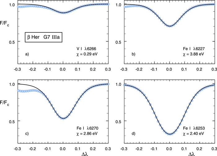
Figure 7. Model profiles (lines) compared to the observations (circles) for a sample of lines. Model profiles have v sin i = 3.27 and ζRT = 6.43 km s−1 as determined from the Fourier analysis (Figure 6).
Download figure:
Standard image High-resolution imageThe rotation rate of 3.27 ± 0.20 km s−1 agrees with the much earlier value of 3.4 ± 0.8 km s−1 (Gray 1982) albeit with significantly smaller uncertainty. The smaller error for the new value reflects primarily the slightly higher resolving power and the much higher S/N of the observations used in the current analysis. The rotation rate of β Her is larger than the values of the K stars measured in Papers 1–3: 1.70 ± 0.20 for β Gem, 2.3 ± 0.2 for ε Cyg, and 2.0 ± 0.3 for α Ser, consistent with the decline toward cooler temperatures documented earlier (Gray 1989).
If we take a radius of 16  , the period of rotation is no greater than ∼250 days or 0.67 years. My observations are too widely spaced to pin down a period this short.
The current value of ζRT = 6.43 ± 0.08 km s−1 is considerably higher than the old value of 4.8 ± 0.4 km s−1 (Gray 1982), but is now more consistent with the general temperature and luminosity dependences for a star between luminosity classes II and III (Gray 2005b, Figure 17.10).
6. BISECTOR SHAPE: THE SECOND SIGNATURE OF GRANULATION
Even though β Her has a higher luminosity than the stars from the previous papers in this series, its λ6253 bisector has the usual C shape, as shown in Figure 8. This is the mean taken over 43 exposures and the horizontal error bars show the standard deviation on this mean. The height or F/Fc value of the blue-most point on the bisector depends on the absolute magnitude of the star. These points are shown by the filled circles on the bisectors. The blue-most point for β Her lies at F/Fc = 0.52 ± 0.02, completely consistent with the absolute magnitude dependence found previously (Gray 2005a, Figure 5).

Figure 8. The λ6253 bisector of β Her is shown with rms deviations as horizontal error bars. Comparable bisectors from Papers 1–3 are shown. Each bisector is shifted in velocity so they match at the low end. Dots on the bisectors are placed at the blue-most points.
Download figure:
Standard image High-resolution image7. CONVECTIVE BLUESHIFTS: THE THIRD SIGNATURE OF GRANULATION
The third signature, a plot of the core line depths as a function of core velocities, is shown in Figure 9. This granulation phenomenon results from the cores of weaker lines being formed deeper in the photosphere where the convective overshoot velocities are larger. The rising hot material dominates the light, producing a net blueshift. Background, discussion, and previous results can be found in earlier publications (Gray 2009; Gray & Pugh 2012, Papers 1–3, and references therein). The data in the figure are comprised of core positions for 36 lines averaged over 35 of the 37 exposures having an absolute velocity scale. (Two were omitted owing to zero level errors in the exposures.) The symbol size reflects the scatter in velocity relative to the exposure mean shown by each line. The average rms error on the points is 16 m s−1. The actual scatter in the third-signature plot is much larger and arises primarily from blends and errors in wavelength calibrations.
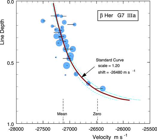
Figure 9. The third signature for β Her. Symbol size is inversely related to the line's observed scatter so larger symbols indicate higher weight. Horizontal tails show the direction and qualitative amount the point would move if the line were unblended. The solid curve shows the adopted scaled standard curve (Gray 2009). The other two curves have scale factors of 1.00, shift of −26590 m s−1 and 1.40, −26370 m s−1. The mean velocity of the measured lines and the zero velocity in the photosphere are shown near the bottom. This convective blueshift amounts to 645 m s−1.
Download figure:
Standard image High-resolution imageThe standard curve (Gray 2009), calibrated against the Sun, is scaled up in velocity by 1.2 ± 0.1 times in order to match the observations. In other words, the granulation velocities in β Her's photosphere are ∼20% larger than in the Sun's. To give some indication of the uncertainty, two additional curves are shown in the figure, one with a scaling of unity and the other with a scaling of 1.4 times the solar scale. A value of 1.2 is consistent with the general rise with effective temperature shown in Gray & Pugh (2012).
The shift of the standard curve in Figure 9 by −26480 with a precision of ±55 m s−1 is an average spectroscopic radial velocity of β Her with the convective blueshifts removed. The absolute calibration of the standard curve is uncertain by an additional ∼50 m s−1. But the −26480 value is for the average of the observed orbital phases. The actual gamma or systemic velocity is −25775 (Table 2) with a precision of ±30 m s−1 and has the additional uncertainty of the standard curve of ∼50 m s−1. The gravitational redshift is expected to be ∼120 m s−1, assuming a mass of three solar masses and a radius of 16 solar radii. The geometric systemic radial velocity, as apposed to the spectroscopic value, would then be ∼120 m s−1 more negative.
8. THE FLUX DEFICIT AND GRANULATION CONTRAST: BISECTOR MAPPING
The change in granulation velocities that produce the third signature will also shape the line bisectors in the same way. On top of that, the imbalance in light coming from the granules and lanes produces further shaping of the bisector. Bisector mapping is a way of extracting some quantitative information about that imbalance. Alterations are made to the observed line profile in such a manner as to reshape the observed bisector to match the third signature for the star. Since λ6253 is both a strong line, which gives a bisector reaching small F/F values, and a line with minimal blending, it is used for the task.
Figure 10 shows the mean observed λ6253 profile for β Her and the modifications made to accomplish the mapping. The difference between the two profiles is the flux deficit. The parallel process with the observed and mapped bisectors is shown in Figure 11. The alterations in Figure 10 produce the bisector changes in Figure 11.

Figure 10. The mapped profile produces the required bisector changes (Figure 11). The deficit is the difference between the profiles, normalized by the profile core depth (0.680).
Download figure:
Standard image High-resolution image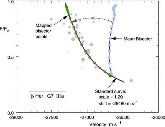
Figure 11. The mean bisector for the λ6253 line is shown with the third-signature points and the standard curve. The points on the bisector are mapped on to the standard curve with the profile alterations in Figure 10.
Download figure:
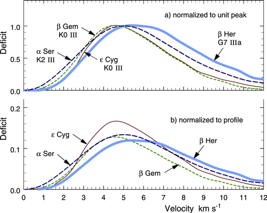
Standard image High-resolution imageThe deficit peaks at 11.9 ± 0.5% of the line's core depth. The deficit for β Her is compared to the results of Papers 1–3 in Figure 12. Even though the third-signature scale values range widely among these stars (0.55 for α Ser to 1.20 for β Her), the flux deficits show relatively small differences. Most notable is the shift of the β Her deficit to higher velocities, peaking about a full km s−1 higher than the others and indicating ∼20% larger average velocity difference between granules and lanes. A wider separation of the granulation "streams" also implies a larger macroturbulence component in the line broadening. Indeed, ζRT = 6.43 for β Her is significantly larger than ζRT = 4.53 for β Gem, 4.30 for ε Cyg, and 4.50 for α Ser. On the other hand, the area of the β Her deficit normalized to half the equivalent width of the line is 12.6 ± 1.0%, indistinguishable from 12.3 ± 1.5% for α Ser or 12.0 ± 1.0% for β Gem. At 14 ± 1%, ε Cyg is also the same or nearly so. It seems that the disk-integrated flux imbalance between granules and lanes is rather stable.
Figure 12. Flux deficits are compared. The deficit for β Her is shifted to higher velocities, but has similar area compared to the others.
Download figure:
Standard image High-resolution image
Based on model photosphere calculations, at the 4990 K effective temperature of β Her, a 12.6% difference corresponds to the granules being 132 K hotter than the lanes. This assumes lanes have the same areal coverage as granules, which is not far from the case for solar granulation (e.g., Sánchez Cuberes et al. 2000). Note that since the fractional deficit area shows only small variation among these stars, the granule–lane temperature differences reflect the the effective temperature. Additional explanation and interpretation of flux deficits can be found in earlier publications (Gray 2010, Papers 1–3).
9. SUMMARY
New high-resolution spectroscopic observations of β Her (G7 IIIa) spanning 10 years are presented and analyzed. A total of 36 radial velocities are measured for this single-line binary and used to derive new orbital elements (Table 2). The orbital results are in excellent agreement with previous determinations, most notably that of Eaton & Williamson (2007). Residual velocities have an rms scatter of 167 m s−1, or about twice the expected value, indicating intrinsic variability. LDRs point to variations ∼2 K over the decade of observation, similar to what is implied by photometric variations. Fourier analysis of 16 lines leads to v sin i = 3.27 ± 0.20 and ζRT = 6.43 ± 0.08 km s−1. This rotation rate agrees with the much older Fourier analysis (Gray 1982) and is consistent with Papers 1–3 as well as the general behavior mapped out in earlier work (e.g., Gray 1982, 1989). The radial–tangential macroturbulence is somewhat higher than previously determined, but agrees well with general trends for its G7 IIIa spectral type. The Fe I λ6253 line bisector has the standard "C" shape with the blue-most point located in the lower half of the bisector, commensurate with the higher luminosity of β Her compared to the stars in Papers 1–3. The third signature of β Her shows a scale factor of 1.20 ± 0.1, implying granulation velocities 1.2 times larger than the solar case. Bisector mapping leads to a flux deficit area of 12.6 ± 1.0% and an estimated temperature difference between granules and inter-granular lanes of 132 K. The shape and position of the flux deficit implies approximately 20% larger velocity difference between granules and lanes compared to the lower luminosity stars measured in the previous three papers of this series.
The third-signature plot is used to convert average measured radial velocities to absolute velocities, that is, velocities with the convective blueshift removed. But note: for a star with a variable velocity, like β Her, the average velocity depends on the timing of the observations. The average absolute velocity given in Section 7 is for the 36 exposures that are analyzed here and is unique to this investigation. This is to be contrasted with the absolute gamma or systemic velocity given in Section 3 (−25775 ms−1), which is the actual blueshift corrected spectroscopic radial velocity of the system.
I am grateful to M. Debruyne for many years of technical support at the Elginfield Observatory where the observations were taken. Thanks to the student observers who took some of the observations. I am grateful to the Natural Sciences and Engineering Research Council of Canada for financial support.