


ABSTRACT
Direct observations of core-collapse supernovae (SNe) and their red supergiant (RSG) progenitors suggest that the upper mass limit of RSGs may be only about  , while the standard theoretical value is as much as
  . We investigate the possibility that RSGs with
  end their lives as failed supernovae (fSNe) and analyze their contribution to the relic supernova neutrino spectrum. We show that adopting this mass limit simultaneously solves both the RSG problem and the supernova rate problem. In addition, energetic neutrinos that originated from fSNe are sensitive to the explosion mechanism, and in particular, to the nuclear equation of state (EOS). We show that this solution to the RSG problem might also be used to constrain the EOS for failed supernovae.
Export citation and abstract BibTeX RIS
1. INTRODUCTION
Although core-collapse supernovae have been investigated numerically for many decades, the detailed explosion mechanism is still unknown (Janka 2012). One reason for this dilemma is that the explosion mechanism is sensitive to details of the nuclear physics and neutrino transport within the SN interior. However, neutrinos generated during the explosion convey valuable information regarding both the macro- and micro-scopic physics of core-collapse SNe due to their unique interactions.
Within this context, there is a useful neutrino resource (Hartmann & Woosley 1997; Hopkins & Beacom 2006) in the spectrum of cosmic relic supernova neutrinos (RSNs). The RSN spectrum consists of the diffuse supernova neutrino background from all types of core-collapse SNe that have occurred throughout cosmic history. This includes not only optically luminous SNe but also optically faint ones that may only be detectable via their neutrino signal. Crucial information regarding the expansion rate of the universe and the cosmic star formation rate (SFR) are all encoded in the redshifted energy spectrum of the RSNs. In this paper we explore the use of the RSN spectrum to understand and simultaneously solve both the red supergiant (RSG) problem and the supernova rate problem.
2. RSG PROBLEM
Interpreting future observations of the cosmic RSN spectrum from high redshift requires an understanding cosmic history. However, the RSN spectrum is also subject to the uncertainties of stellar evolution theory. Many unknown factors contribute to the final stages in the evolution of the massive stellar progenitors for core-collapse SNe.
For example, it is generally accepted that RSGs of 8–25 M⊙ are the progenitors for SNe II, while more massive stars become failed supernovae ultimately forming a black hole. Many numerical investigations have been made in this regard (Hirschi et al. 2004; Woosley & Heger 2006; Sukhbold & Woosley 2013), but these are not yet definitive regarding the mass range of core-collapse SNe progenitors. Indeed, there is recent theoretical evidence (Ugliano et al. 2012; Pejcha & Thompson 2015) indicating that which stars fail and which stars explode is not given by a rigorous progenitor mass cut, but has a complex dependence on stellar structure, mass-loss rate, etc. Hence, even some stars with progenitor masses  (in limited mass ranges) may explode, whereas most other stars form black holes. Nevertheless, for our purposes we adopt the phenomenologically deduced cut off, but allow that some fraction of stars in the upper mass range explode as CCSNe as described below.
However, observational evidence for the mass of SN progenitors has been obtained (Smartt et al. 2009; Smartt 2009) by comparing before and after images of twenty nearby SNe. Surprisingly, this study suggested that the maximum mass of the RSG progenitors of core-collapse SNe may be as small as 16.5 M⊙. This is the so-called a "RSG problem" (Smartt 2009; Smartt et al. 2009). More recently a new study suggests that this value could be as much as 18 M⊙ (Smartt 2015). Although this slightly alleviates the problem this is still much smaller than the theoretically expected value and the RSG problem remains. Moreover, the two limits of 16.5 and 18  arise from two different techniques with their own uncertainties. Hence, we take 16.5–18
  to be a reasonable range of the uncertainty in the lower mass limit for fSNe.
Several solutions to this problem have been proposed (Smartt 2009). Any scenario such as reducing the number of massive RSGs themselves by adopting a steeper initial mass function (IMF), mass loss during RSG evolution, etc. might reproduce the observational results. Among the many ideas to resolve this issue (Smartt 2009), in this paper we consider the possibility that failed supernova explosions occur for massive RSGs with 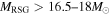 . These supernovae form a black hole and would be optically faint. Nevertheless, they emit a large neutrino flux. Hence, they could be detected, e.g., by a hyper-kamiokande detector (Abe et al. 2011a) via their contribution to the RSN background (Hartmann & Woosley 1997; Hopkins & Beacom 2006; Keehn & Lunardini 2012; Mathews et al. 2014). We investigate this possibility in the following sections.
3. SUPERNOVA RATE PROBLEM
The cosmic supernova rate (RSN) is another valuable means by which to study the evolution of the universe. The determination of this quantity, however, also heavily depends upon the uncertainties of stellar evolution theory. A theoretical evaluation of the cosmic RSN relies on the cosmic SFR, the classification of luminous SNe, and the IMF. Variations in any of these quantities can affect the RSN. Hence, the cosmic RSN is a good testbed for various assumptions. It is described by
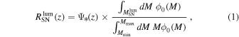
where  is the cosmic SFR, and
  is the IMF. In this paper we adopt the Salpeter-A IMF of Baldry & Glazebrook (2003) (see Section 4). The quantity MSNlum denotes the range of progenitor masses that lead to optically luminous SNe. Hence, RSN depends not only upon the range of stellar masses and the IMF, but also upon the classification of luminous SNe to be discussed in Section 5.
The observationally inferred value for RSN at present (z = 0) is about  (Taylor et al. 2014). Horiuchi et al. (2011) made an extensive study of the RSN. They noticed a tendency for the theoretical RSN to be larger than the observational rate by about a factor of two for SN progenitors classified in the range of
  . This discrepancy is the so-called "supernova rate problem" (Horiuchi et al. 2011). It constitutes an additional dilemma in the understanding of core-collapse supernovae and cosmic evolution.
The RSN is directly related to the neutrino emission during the explosion and affects the RSN background to be discussed in the following section. In our previous paper (Mathews et al. 2014, Paper I) we explored a possible explanation for the supernova rate problem by enhancing the IMF in the range of massive stellar objects. This attempt not only solves the supernova rate problem but also exhibits a distinct signature in the spectrum of energetic relic SN neutrinos depending upon the equation of state (EOS) employed for the SN simulations. This was mainly caused by an excess of fSNe due to an IMF enhancement. Paper I pointed out that the spectrum of RSN could be a valuable tool for an investigation of the nuclear matter EOS. We shall discuss this issue in the following section and show that it remains a valuable tool even in the alternative scenario considered in this paper.
4. COSMIC SFR
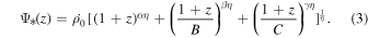
Among the quantities affecting the RSN spectrum, the SFR and the IMF are related to each other. Observational estimates of the SFR depend mainly on the UV emission from galaxies. The UV spectrum, however, is dominated by the contribution from OB stars. One must then extend this information based upon a specific stellar OB population to the entire range of stellar objects in order to get the total SFR, i.e., the gas consumption rate for all star formation. An IMF is assumed for this purpose. The Salpeter-A IMF (Baldry & Glazebrook 2003) for which,

with  (
( ) for stars with
  and
and  (
( ) for stars with
 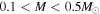 . This is a popular functional form among many IMFs and has been previously used for SFR estimation. We also adopt the Salpeter-A IMF in this paper. We note, however, that the inferred SFR is also affected by dust corrections e.g., (Kobayashi et al. 2000).
Following the formulation given in Yüksel et al. (2008), in Paper I we fitted the cosmic SFR by taking into account these corrections together with new observational data. As in Yüksel et al. (2008), the functional form for the SFR was parameterized as
The fitted parameters for the best fit and their  upper and lower limits in the above expression are summarized in Table 1 (from Paper I). Horiuchi et al. (2011) used a different set of SFR fitting parameters in their identification of the supernova rate problem. As shown in Paper I, the supernova rate problem becomes less pronounced when we apply our SFR formula. This is easily understood since there is a smaller SFR at z = 0 in our case. For consistency with Paper I, we adopt the SFR of Paper I here.
Table 1. Coefficients for the Piecewise Linear Star Formation Rate (Mathews et al. 2014)a,b

|
α | β | γ | B | C | |
|---|---|---|---|---|---|---|
( Mpc−3 yr−1 ) Mpc−3 yr−1 ) |
||||||
| Best Fit | 0.0104 | 4.22 | −0.20 | −11.30 | 2.70 × 10⁶ | 6.37 |
| Upper limit | 0.0200 | 4.22 | 0.14 | −9.0 | 1.25 × 10⁻⁸ | 6.87 |
| Lower limit | 0.0069 | 4.22 | −0.42 | −13.60 | 1.6 × 10³ | 5.90 |
Notes.
aValue of fixed at best-fit value. Smoothing parameter
  adopted from Hopkins & Beacom (2006), Yüksel et al. (2008). Breaks in the spectrum occur at
  and
and ![$1+{z}_{2}=[{C}^{1/(1-\beta /\gamma )}{(1+{z}_{1})}^{(\alpha -\beta )/(\gamma -\beta )}]\approx 4$](https://content.cld.iop.org/journals/0004-637X/827/1/85/revision1/apjaa2a6fieqn24.gif) .
bNote that the wide range of β and B values comes from the wide variation in the slope of the fit at the
.
bNote that the wide range of β and B values comes from the wide variation in the slope of the fit at the  levels.
Download table as: ASCIITypeset image
5. CLASSIFICATION OF SNe
While the RSN is sensitive to the SFR formula, it also depends on the classification of optically luminous SNe. Our SN classification is different from that in the previous work by Horiuchi et al. (2009). This is another aspect of the supernova rate problem.
Stellar evolution calculations are not yet definitive, especially for massive stars. For example, it is difficult to predict which types of progenitors explode as the various observationally characterized types of core-collapse SNe, e.g., Ib,c, IIp, etc. Therefore, we adopt the observationally determined SNe classifications to derive the relic SN neutrino spectrum. Our previous investigation (Paper I) was based upon the assumption that observationally accessible core-collapse SNe occur for progenitors in the mass range of  . We considered
  progenitor stars to be ONeMg SNe, 75% of
  progenitor stars to be SNe II and that 25% of progenitor stars with masses in the range of
  explode as SNe Ib,c. The remaining 75% of progenitor stars with
  were taken to end their lives as fSNe that are too dim to be detected. We numerically treat both SNe II and SNe Ib,c as the luminous core-collapse SNe in the same manner.
According to this classification, one can solve the supernova rate problem with an enhanced IMF for massive stars because it decreases the relative abundance of less massive stars. Since the relative abundance of fSNe increases by this enhancement of the IMF the energy spectrum of RSNs presents a distinct signature depending upon the EOS employed to model fSNe. This result mainly comes from the fact that the neutrinos streaming out from the core of the proto-neutron star in a fSN are much more energetic than those from conventional core-collapse SNe (Sumiyoshi et al. 2005, 2008; Nakazato et al. 2008). Also, their contribution to the spectrum becomes large if an IMF enhancement for massive stars is imposed (Paper I). This study suggested the interesting possibility that one could investigate the SN explosion mechanism through the spectrum of RSNs.
Although this remains a meaningful approach to the supernova rate problem, enhancing the IMF is a bit contrived. It is desirable to keep the IMF conventional, and to solve the supernova rate problem by another means. In this regard, recent new insight has been gained on the massive RSG progenitors of SNe as described in the previous sections. This finding suggests a reclassification of SNe such that all massive stars with progenitor masses of  become fSNe.
Recently, Horiuchi et al. (2014) numerically investigated the fate of massive progenitors. Interestingly they found that progenitors with  tend to fail in successful explosions. This new classification motivated by the RSG problem also increases the relative abundance of fSNe just as in the case of an enhanced IMF. Therefore, it is expected to similarly affect the RSN background. In the next section we numerically analyze this in detail.
6. SN 1978A: BLUE SUPERGIANT (BSG) PROGENITOR
SN 1987A is the nearest and most intensively studied SN. Its progenitor is a BSG star, for which the mass is estimated to be as much as 20 M⊙. Hence, omission of SN 1987A by excluding the massive progenitors with  as luminous SNe raises a question. Several resolutions to this dilemma are possible. For one, the mass of the progenitor for SN 1987A becomes as low as 15 M⊙ in the case of an interacting binary model (Podsiaklowski et al. 1993; Maund et al. 2004). It has also been discussed recently that the observation of oxygen emission lines agrees with the nucleosynthesis model for progenitor masses
  (Jerkstrand et al. 2015). Hence, SN 1987A could be just below our adopted upper mass limit for CCSNe. As another possibility it has been predicted (Pejcha & Thompson 2015) progenitors with
  (or M = 20–21) whereas progenitors of other masses collapse to form black holes. Hence, it is likely that SN 1987A happened to be in the window of exploding progenitors even though the window of BH formation increases with decreasing metallicity. Indeed, the neutrino spectrum from SN 1987A has been used to make earlier estimates of the RSN spectrum. For example, Fukugita & Kawasaki (2003) and Vissani & Pagliaroli (2011) used the spectrum of neutrinos observed to emanate from SN 1987 A to constrain the RSN spectrum.
One might also speculate that the distinct light curve of SN 1987A indicates that this SN may not be an ordinary CCSN but peculiar type, and could represent 3% of all CCSNe (Smartt et al. 2009). However, the neutrino signal from SN 1987A is consistent with a normal core collapse paradigm.
Hence, SN 1987A may be a representative of a class of massive CCSNe that avoids BH formation. It is worth exploring how this class of SNe affects the RSN signal. We discuss this possibility in Section 7 assuming that 3% of progenitors in the mass range  or
or  are SN 1987A-like SNe.
7. DETECTION RATE OF RELIC SN NEUTRINOS
The event rate for terrestrial neutrino detectors can be estimated as follows (Strigari et al. 2005; Yüksel & Beacom 2007).
First, the neutrino number flux per unit energy is determined from
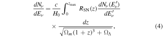
where we adopt  as the redshift at which star formation begins.
  is the neutrino spectrum emitted at the source, and the energy
  is the energy at emission, while Eν is the redshifted energy observed in the detector. Here, we adopt a standard cosmology with
  km s−1 Mpc−1,
  (Horiuchi et al. 2011; Hinshaw et al. 2013). We assume a Fermi–Dirac distribution for all neutrino species.
The total luminosity and temperatures of all SNe are summarized in Table 2 for the two different EOSs for fSNe employed in Sumiyoshi et al. (2008).  is adopted for CCSNe. This value is different from that in Paper I,
  , which was estimated from an average of values from CCSN simulations in the literature. However, a recent comprehensive analysis of SN 1987A (Vissani 2015) supports
  , which is also consistent with the conclusion from a study on the abundance ratio of 180Ta/136La (Hayakawa et al. 2010). Thus we adopt this
  for not only SN 1987A-like objects but also CCSNe of the RSG progenitors. The exact neutrino temperature, however, is not very important. For example, the choice of
  increases the total number of events over a 10 year run by
  . RSN(z) is evaluated by Equation (1), for which we take
  or
or  . The uncertainty in the temperature is evaluated as in Paper I, i.e., the error estimate corresponds to the uncertainty due to the theoretical variation of the neutrino temperatures in time during the explosion.
Table 2. Parameters for the Various Neutrino Sources Considered in this Work
| Detail | SNe(Optically Luminous) | fSNe (Shen EOS) | fSNe (LS EOS) |
|---|---|---|---|
| mass (M⊙) | 10–16.5,18 | 16.5,18–125 | 16.5,18–125 |

|
3.2 ± 0.32 |

|

|

|
4.0 ± 0.50 |

|

|

|
6.0 ± 0.60 |

|

|

|

|

|
 |

|

|

|
 |

|

|

|
 |
Notes. Values for luminous SNe are from Mathews et al. (2014) and those for fSNe are derived from the T50 models in Sumiyoshi et al. (2008). Temperature uncertainty estimated from the time variation of neutrino temperatures during the first few seconds (see the text).
Download table as: ASCIITypeset image
An analysis was made in Totani et al. (1998) of the time dependence of the supernova neutrino temperature based upon the SN explosion model of Mayle et al. (1987) and assuming a Fermi–Dirac neutrino spectrum. In that work it was concluded that after about 1 s the neutrino temperatures only vary by about 10% over the next few seconds when most of the neutrino luminosity is emitted. On the other hand, some of the most recent neutrino transport calculations based upon modern relativistic solutions to the Boltzmann Equation (e.g., Fischer et al. 2012; Roberts et al. 2012) imply smaller average neutrino temperatures and a more rapid decline of temperature with time. Nevertheless, for our purposes we adopt 10% as a reasonable estimate of the uncertainty due to the decline of the neutrino temperatures with time.
The uncertainty in the IMF introduces an overall scaling factor on the cosmic SFR. We estimate this factor as follows. First we assume that the observational cosmic SFR is evaluated based on the UV luminosity from a galaxy mainly emitted by OB stars, the masses of which range from  to
to  . Then, the SFR Ψ is given by

where  is the lifetime of an O5 star, and N0 is a normalization constant. A constant SFR is assumed here. The total observed UV luminosity is similarly obtained by

where LUV(M) is the UV luminosity emitted by a star of mass M. According to these equations, the transformation from a SFR based upon an initial IMF  to a SFR based upon a different IMF
  is given by
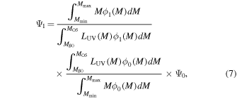
where  and
and  denote SFRs with IMF
  and
and  , respectively. To evaluate LUV(M), we assume
  , which is an empirical fitting formula for main sequence stars in the HR-diagram, and an mass–luminosity relation,
  (cf. Demircan & Kahraman 1991). Teff is the effective surface temperature of the star. We also assume a blackbody spectrum to estimate the UV luminosity by taking
 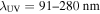 .
.
With this scaling factor and the uncertainty of RSNobs we deduce the ratio of the theoretical to observed supernova rate to be  for
for  (≈0.85–1.35 for
  ).
).
This means that the supernova rate problem is almost solved simultaneously with the RSG problem. Figure 1 shows the dependence on the minimum mass of the failed supernova progenitor MminfSN. Figure 1 demonstrates that the effect is not large.

Figure 1. Relationship between MfSNmin and  . Two cases displayed by red and green curves are for the different cosmic SFRs from Mathews et al. (2014, Paper I) and Horiuchi et al. (2011), respectively. Upper and lower dotted curves show the error bands arising from the uncertainties in the observed cosmic SFR and IMF as described in the text. The vertical lines indicate the adopted range of the lower mass limit for fSNe. The horizontal blue band indicates the range of uncertainty caused by RobsSN.
Download figure:
Standard image High-resolution imageThe detector event rate is

where Ntarget is the number of target particles in the detector,  is the cross section for neutrino interactions within the detector (Strumia & Vissani 2003), and
  . Here, we consider the neutrino absorption to be dominated by the
  reaction.
Figure 2 shows the event rate of RSNs assuming 10 years of running time in a Hyper-Kamiokande detector, i.e., a 106 ton water Čerenkov detector (Abe et al. 2011a). This figure includes cases in which different models for fSNe are chosen in order to illustrate the EOS dependence of fSNe. We adopt the previous numerical models for fSNe by Sumiyoshi et al. (2008) that utilized both a soft EOS (i.e., the K = 180 LS-EOS; Lattimer & Swesty 1991) and a stiff EOS (i.e., the Shen-EOS, Shen et al. 1998). We assume zero chemical potential for neutrinos. Then, the luminosity  and averaged energy
  are described by

and

where

Applying these expressions to the time-evolution of both the luminosity and averaged energy (Sumiyoshi et al. 2008) we find the neutrino temperature T(t) and the radius of the neutrino sphere R(t), and deduce an instantaneous energy spectrum given by
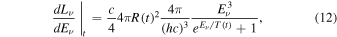
where the time-dependence is shown explicitly.
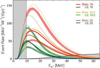
Figure 2. Predicted  energy spectra and uncertainties in the total SRN detections for the cases of
  or
or  . No neutrino oscillation is considered. The uncertainty bands are based upon the observed cosmic SFR and the detector statistics. Thick lines are for the best-fitted observed cosmic SFR. Thin lines show the upper and lower-limits of the SFR. For purposes of illustration, the error band is only shaded for the case of
  for illustrative purpose. The results for two different fSNe models based upon the stiff EOS of Shen et al. (1998) and the soft EOS of Lattimer & Swesty (1991) are included. The shaded energy range below 10 MeV indicates the region where the background noise due to reactor
  may dominate. The shaded energy range that intersects the spectrum at ∼34 to 46 MeV indicates the region where the background may be dominated by noise from atmospheric neutrinos.
Download figure:
Standard image High-resolution imageWe then integrate over time to obtain the total energy spectrum and fit it with a Fermi–Dirac distribution to estimate the effective temperature for each neutrino species. Total luminosities are utilized as constraints for the fitting procedure. The total energies and adopted temperatures for the various components are summarized in Table 2. From this table it is clear that fSNe are a more energetic neutrino source although they are not optically luminous due to the formation of the black hole.
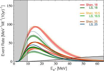
As for the neutrino oscillation pattern induced by the matter effect (Dighe & Smirnov 2000), there are two possible cases according to the classification introduced in Paper I, i.e., either a normal or inverted mass hierarchy associated with complete non-adiabatic mixing (Case I) or an inverted mass hierarchy associated with complete adiabatic mixing (Case II) through the MSW high-density resonance. In Case I, the detected flux would be

while in Case II, if there is no effect from shock wave propagation which may induce non-adiabatic transition, the flux would be

Since it is known that the  mixing angle is as large as
  (An et al. 2012),
  (Ahn et al. 2012),
  (Abe et al. 2012), which is consistent with
  (Abe et al. 2011b), one can expect a complete swap of energy spectra between
  and
and  as in case II defined above. Figures 2 and 3 show the calculated results without and with the effects of neutrino oscillations, respectively, for this case of an inverted mass hierarchy and complete adiabatic mixing. In these figures we include the LS and Shen-EOS for fSNe. Three different scenarios are shown, for which use
  or
or  . Here, we do not show the Case I result because it is similar to the results without oscillation (within 30%) at low energies including the peak as is evident from the above expression. The high energy part is slightly different in the two cases, but the atmospheric neutrino background obscures the interesting difference between the two cases.
Figure 3. Same as Figure 2, but with the neutrino oscillations included for the case of complete adiabatic mixing.
Download figure:
Standard image High-resolution image
As mentioned in Section 6, there might be a SN 1987A-like BSG progenitor in the mass range up to  . It is likely, however, that they do not influence the SRN spectrum significantly and their effect is not discernible when we allow the possibility that 3% of the progenitors in the mass range are SNe of this type. The total event numbers above the atmospheric background are summarized in Tables 3 and 4.
Table 3. Total Events Over 10 years Running Assuming the Shen-EOS
| w/o Osc. | w Osc. | |||||
|---|---|---|---|---|---|---|
| MRSGmax (M⊙) | 16.5 | 18 | 25 | 16.5 | 18 | 25 |
| Best fit | 1595 | 1447 | 1023 | 967 | 937 | 856 |
| Upper limit | 3108 | 2827 | 2013 | 1924 | 1862 | 1691 |
| Lower limit | 981 | 888 | 626 | 582 | 565 | 519 |
Note.
Upper and lower limits are variations.
Download table as: ASCIITypeset image
Table 4. Total Events Over 10 years Running Assuming the LS(220)-EOS
| w/o Osc. | w Osc. | |||||
|---|---|---|---|---|---|---|
| MRSGmax (M⊙) | 16.5 | 18 | 25 | 16.5 | 18 | 25 |
| Best fit | 524 | 512 | 478 | 546 | 569 | 635 |
| Upper limit | 1032 | 1007 | 935 | 1089 | 1131 | 1253 |
| Lower limit | 322 | 315 | 296 | 328 | 343 | 387 |
Note.
Upper and lower limits are variations.
Download table as: ASCIITypeset image
The event rate based upon fSNe with the Shen-EOS overwhelms the case of the soft LS-EOS. In general, a stiff EOS leads to a larger mass of accreted material onto the proto-neutron star. This implies a longer duration of the neutrino burst before collapse to a black hole. Increasing the relative abundance of fSNe boosts the number of energetic neutrinos. This makes for a distinct EOS dependence, although the two cases significantly overlap each other when including error bands. These arise mostly from the uncertainties of the observed cosmic SFR in addition to the detector statistics, particularly in the lower energy range. This feature is basically the same as that reported in Paper I except for the magnitude of the event rates. We also note that in this figure the contributions from the LS and Shen EOS are opposite to that of Paper I due to a mislabeling of the similar figure in that paper.
More importantly, however, there is another intriguing aspect in the RSN spectrum seen in the high energy tail. The locations where the event rates exceed the atmospheric background are well separated. Therefore, a detection of the RSN spectrum can give insight into the SN explosion mechanism in terms of the nuclear matter properties.
Finally, we comment briefly about the same calculation with the SFR of Horiuchi et al. (2009). With the same value for MSNlum, the separation between the spectra in the lower energy range for the different EOSs becomes much larger than in the present work. A higher value of  for their SFR explains this trend. However, neither 16.5 nor
  for the upper limit of MSNlum are low enough to solve the supernova rate problem entirely for the Horiuchi et al. (2009) SFR while the combination of the SFR and MSNlum in this paper solves both problems together (see Figure 1). Although this result is intriguing, it is important to keep in mind that more accurate observational data for the cosmic SFR is needed to make a definitive explanation of the SN-rate problem.
8. CONCLUSION
We have adopted a new parameterization for the SFR along with the assumption that fSNe occur for progenitors with masses above  . This scheme provides a simultaneous solution to both the supernova rate problem and the RSG problem. Moreover, the RSN spectrum based upon this is sensitive to the nuclear matter EOS inside the core, and thereby offers a possible means to gain insight into the physics of core-collapse supernovae.
We thank K. Sumiyoshi and T. Yoshida for productive suggestions. This work was supported in part by Grants-in-Aid for Scientific Research of JSPS (26105517, 24340060) of the Ministry of Education, Culture, Sports, Science and Technology of Japan. Work at the University of Notre Dame (GJM) supported by the U.S. Department of Energy under Nuclear Theory Grant DE-FG02-95-ER40934.