
Multi-Terminal DC Grid with Wind Power Injection
by
 , , and
Lilantha Samaranayake
1,* ,
,
Carlos E. Ugalde-Loo
2,
Oluwole D. Adeuyi
3,
John Licari
4 and
Janaka B. Ekanayake
2 1
Faculty of Engineering, University of Peradeniya, Peradeniya 20400, Sri Lanka
2
School of Engineering, Cardiff University, Wales CF24 3AA, UK
3
SSE Renewables, Waterloo Street, Glasgow G2 6AY, UK
4
Faculty of Engineering, University of Malta, MSD 2080 Msida, Malta
*
Author to whom correspondence should be addressed.
Wind 2022, 2(1), 17-36; https://doi.org/10.3390/wind2010002
Submission received: 27 October 2021
/
Revised: 31 December 2021
/
Accepted: 4 January 2022
/
Published: 7 January 2022
Abstract
:With the development of offshore wind generation, the interest in cross-country connections is also increasing, which requires models to study their complex static and dynamic behaviors. This paper presents the mathematical modeling of an offshore wind farm integrated into a cross-country HVDC network forming a multi-terminal high-voltage DC (MTDC) network. The voltage source converter models were added with the control of active power, reactive power, frequency, and DC link voltages at appropriate nodes in the MTDC, resembling a typical cross-country multi-terminal type of HVDC scenario. The mathematical model for the network together with the controllers were simulated in MATLABTM and experimentally verified using a real-time digital simulator hardware setup. The resulting static and dynamic responses from the hardware setup agreed well with those from simulations of the developed models.
1. Introduction
The goal to limit climate-change-induced temperature increases to 1.5 °C is at best uncertain, with analyses predicting that even with the implementation of the current commitments [1,2,3], the global average temperature increase will be close to 2.4 °C and will be catastrophic for environmental systems. While technological developments to replace fossil-fuel-based energy systems are challenging, it is becoming increasingly clear that decarbonizing electricity grids is a must. During this journey, the development of renewable energy sources (RESs) both onshore and offshore will play a key role. Of the different RESs, the offshore wind capacity continues to increase and was not impacted by the COVID-19 pandemic. In 2020, more than 6 GW of offshore wind power capacity was added globally, bringing the cumulative global capacity to 34 GW. It is expected that approximately 83 GW of offshore wind will be connected to the North Sea regional grid in Europe by 2030 [4,5].
When considering offshore wind farms, the challenge lies in how this wind power can be harvested efficiently, in terms of both cost and performance. The extent of the challenge is largely dependent on the scale of the project considered, pace of growth and the distance at which it is to be located offshore. In fact, many of the largest wind farms are located at considerable distances from shore. This causes problems in the transmission of energy using conventional high-voltage alternating current transmission cables, because the capacitance of the cables causes excessive charging currents, leaving less capacity for useful current flow [6,7,8,9]. High-voltage direct current (HVDC) transmission, by its very nature, does not involve oscillatory charging currents. As such, it has been thoroughly explored as a solution to overcome the limitations of AC connections for offshore wind farms [10,11].
With the development of offshore wind generation, the interest in cross-country connections is also increasing. The Airtricity Foundation proposes a 10 GW offshore wind farm (OWF) located between the UK, Germany, and the Netherlands as a foundation project for a European supergrid [12]. Greenpeace suggests approximately 65 GW of offshore wind capacity to be connected to 7 countries [13]. Seven European transmission system operators have signed a Memorandum of Understanding for the launch of Eurobar, an initiative for interconnecting offshore wind platforms across Europe [14]. Even though many possible options are available for these cross-country connections, multi-terminal high-voltage DC (HVDC) grids (MTDC) that utilize voltage source converters (VSCs) have been widely investigated [13,14,15,16,17,18].
Current XLPE cable technology permits voltages of up to 420 kV AC for single-core cables and 275 kV AC for triple-core cables. Although single-core cables typically provide higher ratings, three separate conductors must be laid, which increases the installation costs [19]. Compared to AC connections, HVDC requires a lower number of cables and for the distances associated with cross-country connections, while limitations due to increased capacitance generating a large amount of reactive power along the cable’s length do not exist.
If more offshore wind farms and countries are connected through MTDC networks, the resulting DC grid could be very complex, requiring models to study the static and dynamic behaviors. Even though the connections can be complex, the basic building blocks of the network will involve AC grids to which the MTDC network is connected through VSCs, wind farms, and HVDC lines. In order to study the dynamic behavior of MTDC grids, it is essential to develop mathematical models for these building blocks. In [20], a small-signal model of a voltage source converter-based multi-terminal direct current system was presented by constructing a non-linear state-space model and linking equations for each subsystem. Step-by-step modeling of the MTDC network using average-value models of VSCs with a systematic approach for steady-state and dynamic operation studies was presented in [21]. Based on the small-signal model, the coupling mechanism between converter stations and on the AC/DC side of the converter stations in a VSC-MTDC was presented in [22]. In addition, such models have been presented in [23,24,25,26,27]. However, their validation for MTDC networks, especially using a prototype, is not found in the literature. Furthermore, such models are not used to assess the capacity of wind farms that can be connected to MTDC networks.
In this paper, grid component models are developed from the first principles to investigate MTDC grids, which are validated using a scaled-down three-terminal MTDC test rig. Dynamic studies are carried out to assess the stability of the MTDC network with wind power injection, and the stability is also demonstrated using a case study. Although the case study involves a simplified network, the approach followed in this work enables future system expansion for more detailed studies. Mathematical modeling is carried out in MATLAB using state-space representations suitable for small-signal stability assessments through eigenvalue analysis.
To validate these results, the system is implemented on a scaled-down experimental three-terminal MTDC test rig. The experimental results show good consistency with the eigenvalue analysis.
In this paper, Section 2 highlights the development of modeling tools from fundamentals, while Section 3 covers the hardware-in-the-loop experimental verification of the modeling tools developed in the previous section. The results of the experimental verification of the modeling tools presented and discussed in Section 4 and the conclusions are presented in Section 5.
2. System Modeling Tools
In this section, we develop modeling tools consisting of state-space models of the fundamental components of wind-farm-connected MTDC networks. The modeling will include:
- A wind farm with an AC-to-DC converter for frequency control and reactive power flow control;
- A grid-connected converter to control the DC link voltage and reactive power flow;
- A grid-connected converter to control the active power flow and reactive power flow;
- The models for points 2 and 3 above are similar up to the inner current control, with only the outer most control loops differing.
2.1. Wind Farm with AC-to-DC Converter for Frequency Control and Reactive Power Flow Control
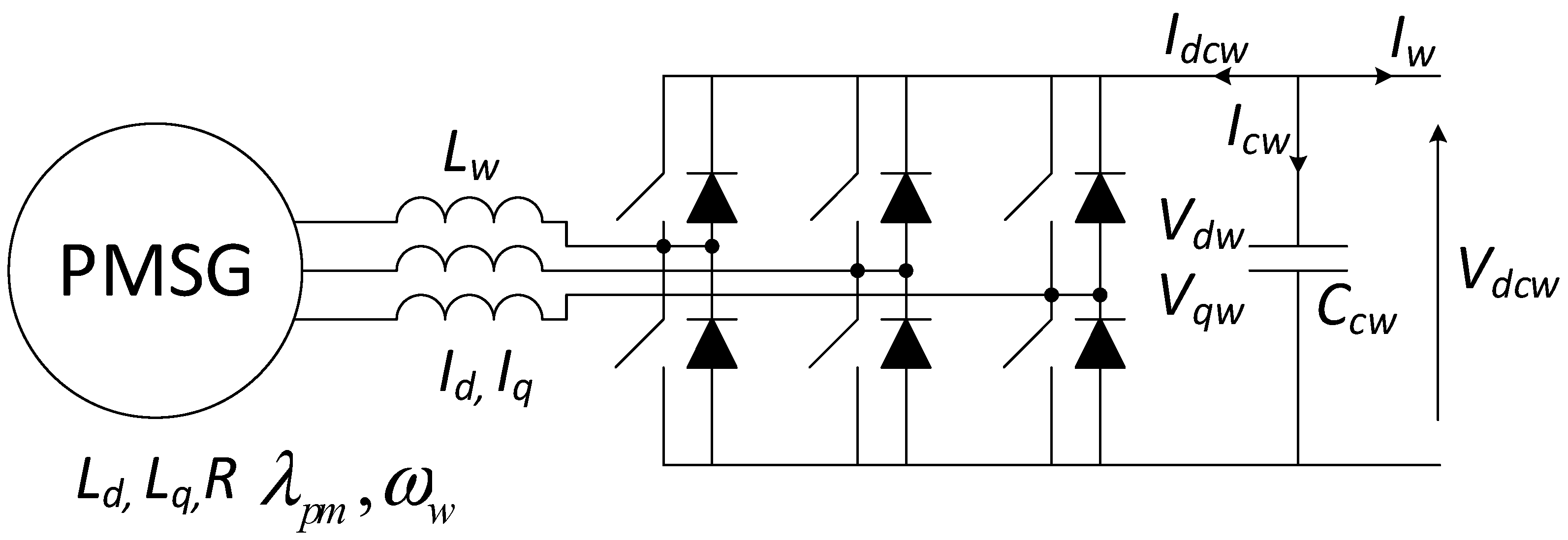
In this section, a model of a wind farm scenario based on wind turbines equipped with a permanent magnet synchronous generator (PMSG) is considered. The PMSG is mechanically connected to a wind turbine and is electrically connected to a transmission line. The other end of the transmission line is connected to an AC-to-DC converter. The output of the AC-to-DC converter is connected to the DC grid. The corresponding configuration is shown in Figure 1.
The fundamental voltage relationships were derived for each component as outlined below.
2.1.1. PMSG, Transmission Line, and Converter Model
Inner current controllers consisting of proportional and integral controllers were introduced to the d and q loops as follows:
where:
and = respective dq reference currents;
and = proportional and integral gains, respectively, of the controller on the d-axis;
and = proportional and integral gains, respectively, of the controller on the q-axis.
The outer control loops for frequency control and reactive power flow control were introduced as:
where Q is the reactive power, Qref is the desired reactive power, f is the frequency, and fref is the desired frequency.
2.1.2. Rotor Dynamics Model
For the PMSG, the rotor dynamics can be given by:
Since , (8) was written as:
Assuming that the PMSG is a non-salient pole type, the induced torque was written as:
Hence:
2.1.3. Reactive Power Dynamic Model
The reactive power was expressed as:
Since and Equation (12) was modified as:
Assuming that Vdcw can reach Vdcwref fast enough, then:
By taking the first derivative with respect to time:
2.1.4. DC Link Voltage Dynamic Model
By taking the active power in the converter on AC side and DC side into consideration and assuming a loss-less converter, then:
By using the definitions of the modulation indexes, then:
With and since the DC link capacitor , the DC link dynamic model becomes:
2.1.5. State-Space Model of the Wind Farm with AC-to-DC Converter for Frequency Control and Reactive Power Flow Control
In order to simplify the PI controllers, four new state variables were defined as:
, ,
and .
Then, by defining the states as:
and the input as
, the state-space model of the wind farm with the AC-to-DC converter for frequency control and reactive power flow control can be simplified. The state equations are given in (19) to (27):
2.2. Grid-Connected Converter to Control the DC Link Voltage and Reactive Power Flow
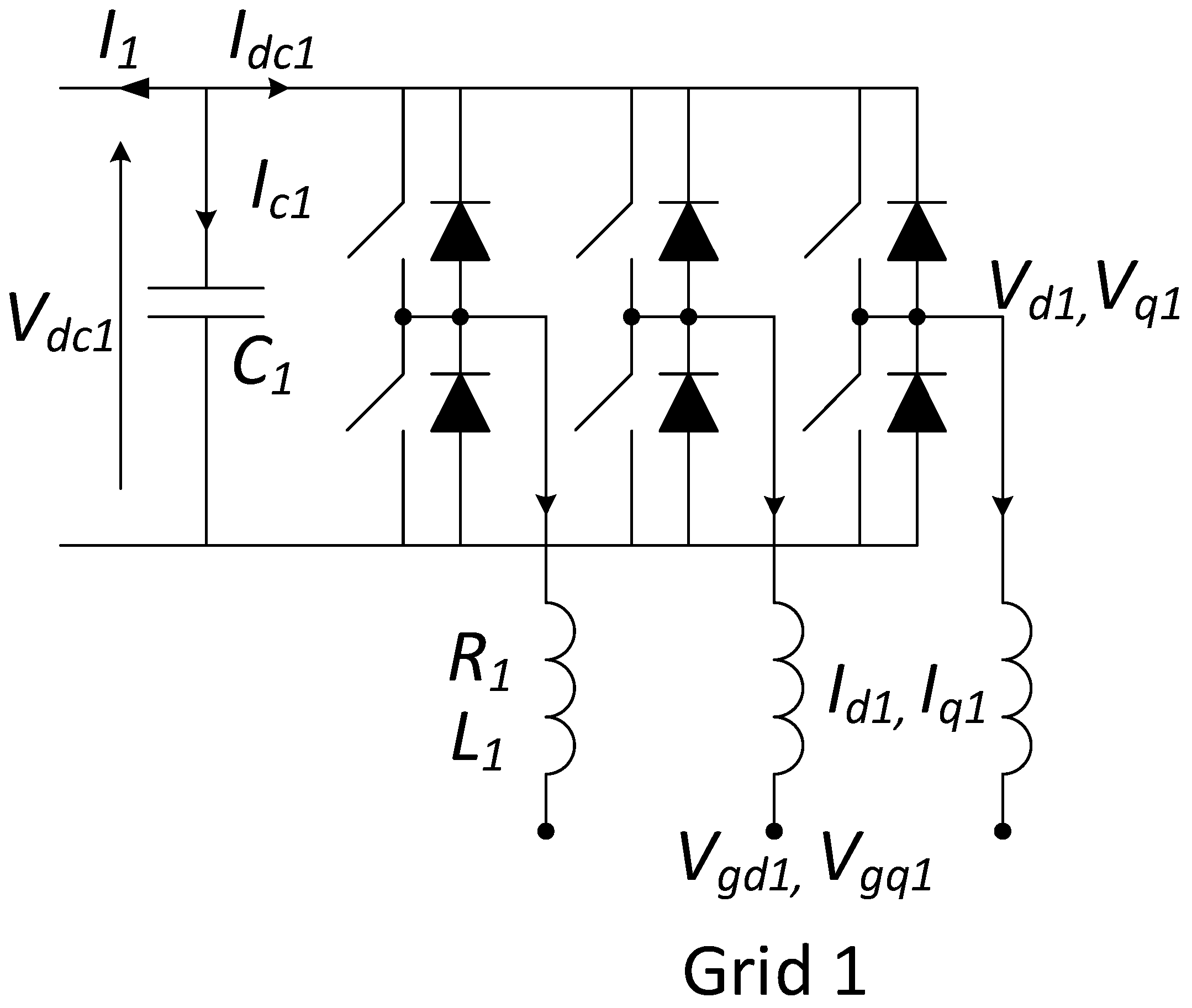
This setup consists of the DC–AC converter, where the DC side is connected to the MTDC network and the AC side is connected to a transmission line. The other end of the transmission line is connected to an AC power grid, as shown in Figure 2.
2.2.1. Grid-Connected Transmission Line Model
The following equations were obtained in the dq reference frame:
2.2.2. Inner Current Controller Model
The inner current controllers formed using PI controllers were obtained as:
where:
and = respective dq reference currents;
and = proportional and integral gains of the controller on the d-axis;
and = proportional and integral gains of the controller on the q-axis.
2.2.3. DC Link Voltage and Reactive Power Flow Controller Model
The current references were obtained using a PI controller as:
where Q1 is the reactive power, Q1ref is the desired reactive power, Vdc1 is the grid side DC link voltage, and Vdc1ref is the desired grid side DC link voltage.
The derivations of the dynamic models of reactive power flow and the DC link voltage were obtained following a similar procedure to those presented in Section 2.1.3 and Section 2.1.4, respectively. The respective dynamic models are:
2.2.4. State-Space Model of the Grid-Connected Converter Used to Control the DC Link Voltage and Reactive Power Flow
As in the previous case, to simplify the PI controllers, four new state variables were defined as:
; ;
; .
Then, by defining the states as:
and the input as
, the state equations were obtained as in (36) to (43):
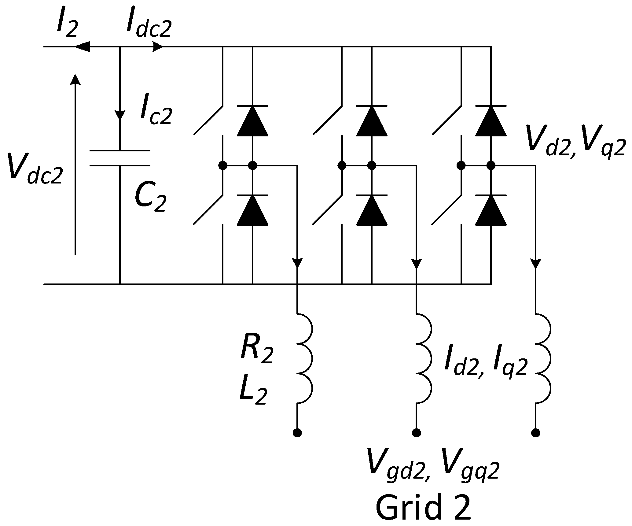
2.3. Grid-Connected Converter Used to Control the Active Power Flow and Reactive Power Flow
The setup shown in Figure 3 is exactly the same as in Section 2.2, except that the DC link voltage control in the outer loop is replaced with the active power flow control. Therefore, all derivations up to the inner current control are the same except for the use of subscript 2 in place of subscript 1. However, the outer most control loop consists of active power flow control.
2.3.1. Active Power and Reactive Power Controller
The current references were obtained using a PI controller as:
where Q2 is the reactive power flow and Q2ref is the desired reactive power flow, while P2 is the active power flow and P2ref is the desired active power flow of the converter.
2.3.2. Active Power Dynamic Model
The active power flowing to the grid is expressed as:
By considering the d and q axis modulation indexes () of the converter are as follows:
Assuming that Vdc2 reaches Vdc2ref fast enough:
By taking the time derivative:
2.3.3. State-Space Model of the Grid-Connected Converter to Control the Active Power Flow and Reactive Power Flow
To simplify the PI controllers, four new state variables were defined as:
; ;
; .
By choosing the state vector as and the input vector as , the state equations were obtained as in (50) to (58):
3. Hardware-in-the-Loop Experimental Verification of Modeling Tools
Next, the models derived in Section 2 were experimentally verified using a hardware-in-the-loop test-rig. These were referred to as:
- WFC: Wind farm with AC-to-DC converter with frequency control and reactive power control;
- GSC 1: Grid-connected converter used to control the DC link voltage and reactive power flow;
- GSC 2: Grid-connected converter used to control the active power flow and reactive power flow.
These were in the same order as those derived in the Section 2. Figure 4 shows the overall hardware system block diagram, which corresponds to the MTDC network. Different configurations such as GSC1 only, GSC1 connected to GSC2, GSC1 connected to WFC, and GSC1 connected to GSC2 and WFC were used to highlight the respective controller implementations in the model verification process.
3.1. Hardware-in-the-Loop Experimental Setup
The main components of the hardware-in-the-loop (HIL) experimental platform are shown in Figure 5. These comprise a real time digital simulator (RTDS), a grid simulator (GS), and an HVDC test rig.
3.1.1. Main AC Grid Model in RTDS
For simplicity, the mainland AC grid was modeled as a 400 kV single-bus system connected to a load and a fault resistance instrument using the RSCAD software in RTDS. However, this network can be easily expanded to represent generators, loads, transformers, and transmission lines of more complex AC systems.
3.1.2. Grid Simulator
The major function of the grid simulator is to produce a three-phase mains supply voltage from the analog outputs of the RTDS. This is achieved using a four-quadrant amplifier rated at 2 kVA and 270 V (L-G rms). In this study, the output of the grid simulator was connected to the DC GSC1 of the HVDC test rig.
3.1.3. Three-Terminal HVDC Test Rig
The AC grids were represented using a 415 V AC mains supply. An autotransformer was used to regulate the supply voltage of the grid-side converter (GSCs) to 140 V. The wind farm was implemented using a motor–generator set with permanent magnet synchronous machines.
The motor torque, T3, was controlled using a UnidriveTM inverter. The reference torque was multiplied by a droop gain, kT, with a droop constant of 0.001. The output of the droop gain was fed through a rate limiter with a slew rate of ±0.5. The generator’s synchronous speed was controlled using the WFC, as illustrated in Figure 4. The DC cable parameters shown in Figure 4 were L23 = 2.4 mH, R23 = 0.045 Ω, L13 = 3.4 mH, R13 = 0.064 Ω. Figure 5 shows the hardware setup.
3.2. Controllers
The implementation of the controllers in GSC1, GSC2, and WFC is presented in this section.
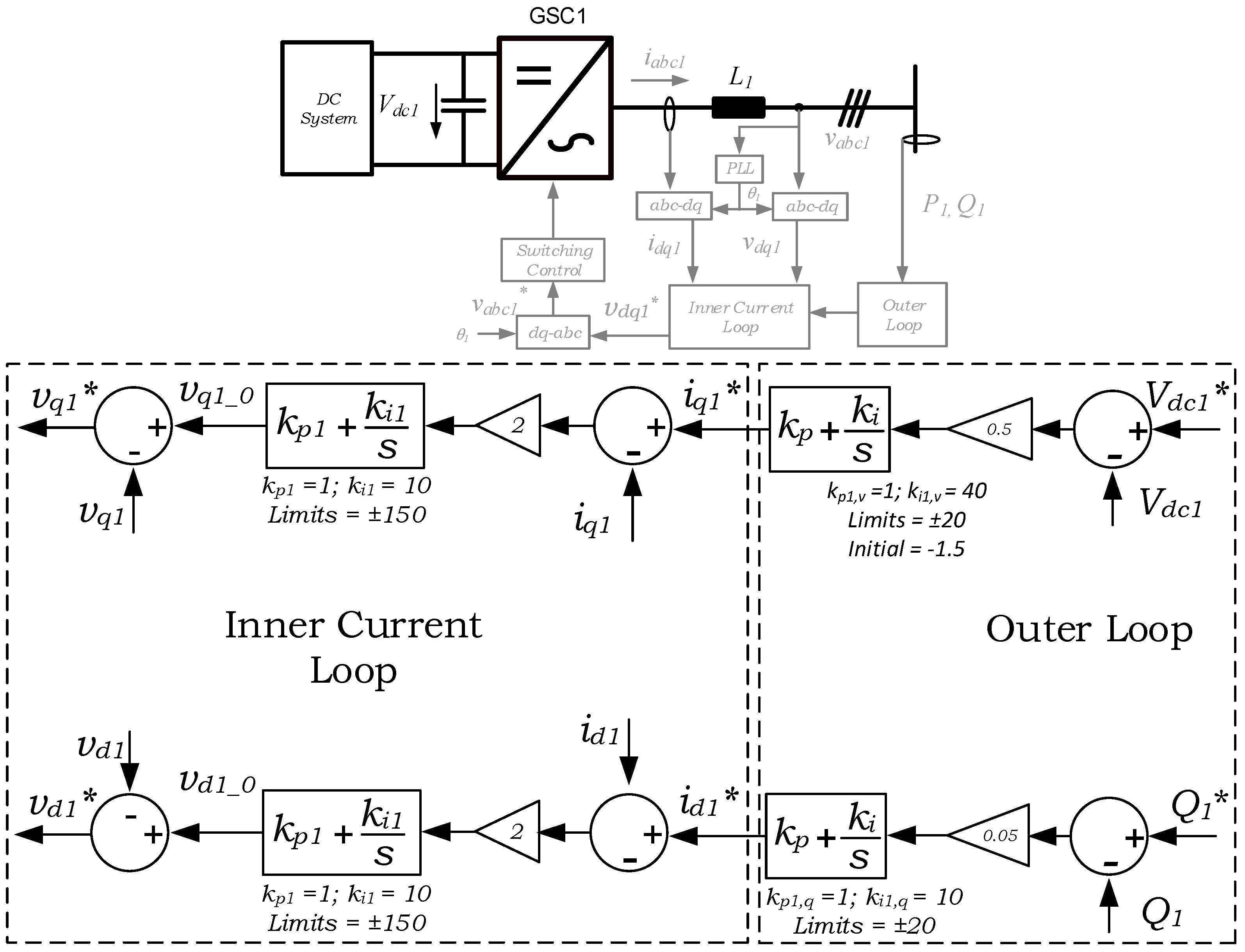
3.2.1. DC Link Voltage and Reactive Power Controllers
Figure 6 shows the DC link voltage and reactive power control scheme for GSC1. This consists of the inner current control loops in the dq-reference frame. The outer control loop provides the references for the inner current controllers. As such, the outer DC link voltage () control loop provides the q-axis current reference and the outer reactive power () control loop provides the d-axis current reference. The and are the ac voltages and currents in the three phases and .
The reference value of DC link voltage, Vdc1*, is compared with its actual value, Vdc1. The error between the two DC voltages is fed to a proportional gain, whose output is processed using a PI controller. The output of the PI controller is the reference q-axis current, iq1*, flowing through the inductance, L1, of the GSC1.
The iq1* is compared with the actual q-axis current, iq1. The error between the two current signals is fed to a proportional gain, whose output is processed using a PI controller. The output of the PI controller is a voltage signal, vq1_0, which is compared with the measured q-axis voltage, vq1, in order to compute the reference q-axis voltage, vq1*.
The reference reactive power, Q1*, is compared with its actual values, Q1. The error between the two reactive power signals is fed to a proportional gain, whose output is processed using a PI controller. The output of the PI controller is the reference d-axis current, id1*, flowing through the AC grid inductance, L1.
The id1* is compared with the actual d-axis current, iq1. The error between the two current signals is fed to a proportional gain, whose output is processed using a PI controller. The output of the PI controller is a voltage signal, vd1_0, which is compared with the measured d-axis voltage, vd1, in order to compute the reference d-axis voltage, vd1*.
3.2.2. Active and Reactive Power Controllers
Figure 7 shows the active power and reactive power controllers for GSC2. The active power, P2, is controlled using the q-axis, while the reactive power, Q2, is controlled using the d-axis.
The reference value of active power, P2*, is compared with its actual value, P2. The error between the two active power signals is fed to a proportional gain, whose output is processed using a PI controller. The output of the PI controller is the reference q-axis current, iq2*, flowing through the inductance, L2, for GSC2. The iq2* is compared with the actual q-axis current, iq2. The error between the two current signals is processed using a PI controller, whose output is added to a term Lq.iq2, to produce a voltage signal, vq2_0, as shown in Figure 7. The vq2_0 is compared with the measured q-axis voltage, vq2, in order to compute the reference q-axis voltage, vq2*. Similarly, the reactive power loop is used to in order to compute the reference d-axis voltage, vd2*.
3.2.3. Frequency Controller and Reactive Power Controller
Figure 8 shows the wind farm frequency and reactive power controller of the wind farm converter. The frequency is controlled using the q-axis and the reactive power is controller using the d-axis. The reference value of offshore frequency, f *, is compared with the actual frequency, f, of the synchronous generator. The error between the two signals is fed to a proportional gain, whose output is processed using a PI controller. The output of the PI controller is the reference q-axis current, iq*.
Here, iq* is compared with the actual q-axis current, iq. The error between the two current signals is fed to a proportional gain, whose output is processed using a PI controller. A cross-coupling term, is added to the PI controller output, vq, to compute the reference q-axis voltage, vq*, where Lq is the q-axis inductance of the PMSG. The reactive power controller has a similar design as the grid-side converter computing the reference d-axis voltage, vd*.
4. Results and Discussion
In this section, the simulation results are compared against the experimental results for verification of the four cases, namely GSC1 only, GSC1 connected to GSC2, GSC1 connected to WFC, and GSC1 connected to GSC2 and WFC.
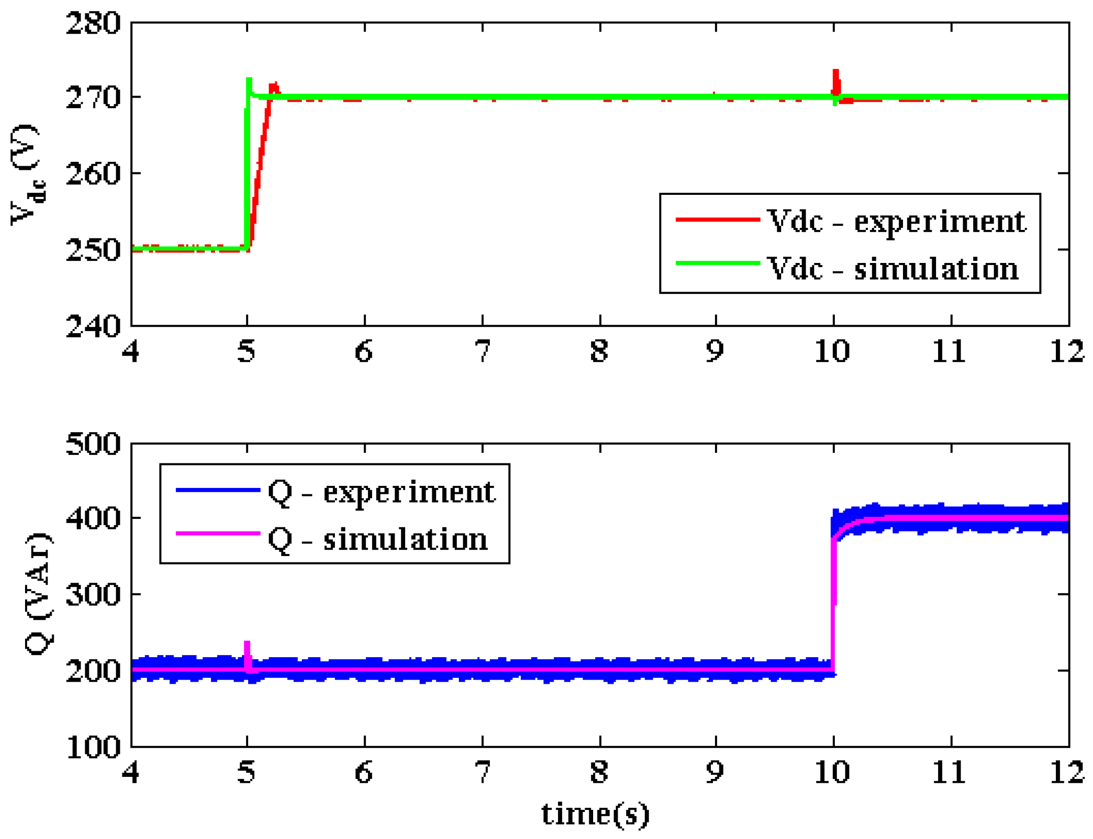
4.1. Verification 1: GSC1 Only
The objective of this verification step was to verify the DC link voltage and reactive power flow control implementation of GSC1. In the test, the following step changes were applied:
- Step change in DC voltage reference, Vdc1*, from 250 V to 270 V at t = 5 s;
- Step change in reactive power reference, Q1*, from 200 VAr to 400 VAr at t = 10 s.
The resulting Vdc1 response to the step change in Vdc1* is shown in the upper part of Figure 9. Further, the resulting Q1 response to the step in Q1* is shown in the lower part of Figure 9.
It can be observed that the Vdc1 follows the reference Vdc1* in principle, although the experimental transient results are slower than the simulation model results in the step change, which may be attributed to possible parameter mismatches in the controller implementations. However, this trend is not prominent in the Q1 response, which follows the reference well. In addition, the dq cross-coupling is present to different degrees in the two cases. In the Vdc1 control, cross-coupling in the simulation is lower than the experimental corresponding to the step change in Q1*. In the Q1 control, however, the cross-coupling in the simulation is larger than in the experiment.
4.2. Verification 2: GSC1 Connected to GSC2
The objective of this verification step was to test the active power and reactive power flow control implementation for GSC2. The following step changes were applied:
- Step change in active power reference, P2*, from 100 W to 600 W at t = 5 s;
- Step change in reactive power reference, Q2*, from 100 VAr to 600 VAr at t = 10 s.
The resulting P2 response to the step change in P2* is shown in the upper part of Figure 10. Further, the resulting Q2 response to the step in Q2* is shown in the lower part of Figure 10.
As observed in Figure 10, both controllers follow their respective references. The simulated P2 response is faster and with virtually no overshoot, while the experimental version has non-zero overshoot that is not significant. In addition, the dq cross-coupling is also present. However, the Q2 responses in the simulation and experiment are similar, with no overshoot or cross-coupling. Hence, the mismatches in the former case may be attributed to possible parameter mismatches and unmodeled dynamics.
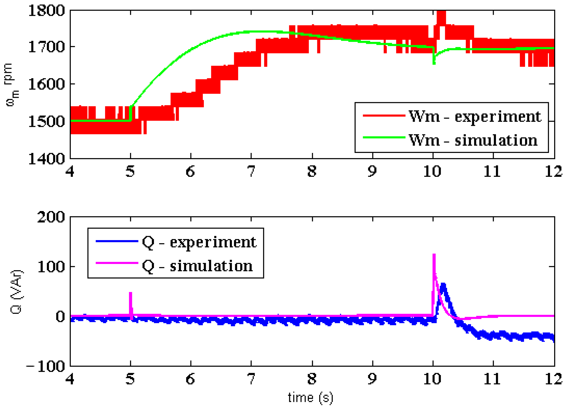
4.3. Verification 3: GSC1 Connected to WFC
The objective of this verification step was to test the AC frequency control and wind turbine torque control implementation for WFC. The following step changes were applied:
- Step change in frequency reference, f3*, from 75 Hz to 85 Hz at t = 5 s.
- Step change in torque reference, T3*, from 5.6 Nm to 10 Nm at t = 10 s.
The resulting f2 response, which is observed as the mechanical shaft speed ωm response to the step change in f3*, is shown in the upper part of Figure 11. The operation of the Q2 controller is shown in the lower part of Figure 11, which is achieved by holding its reference despite the change in the input torque.
In this verification step, the f2 control and Q2 control follow their respective references. The experimental f2 transients are slower, most probably because of unmodeled dynamics in the experimental setup. In addition, the dq cross-coupling is also present in both scenarios.
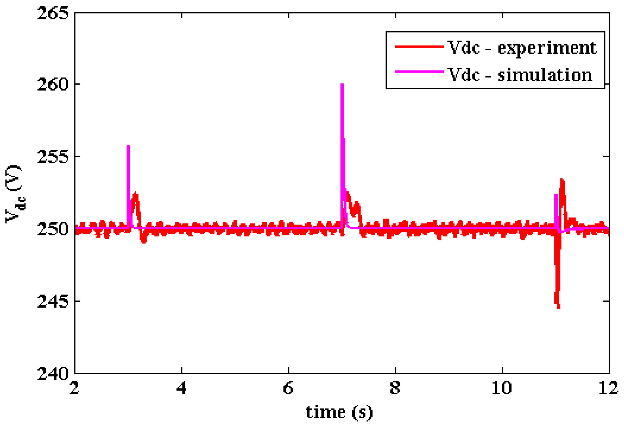
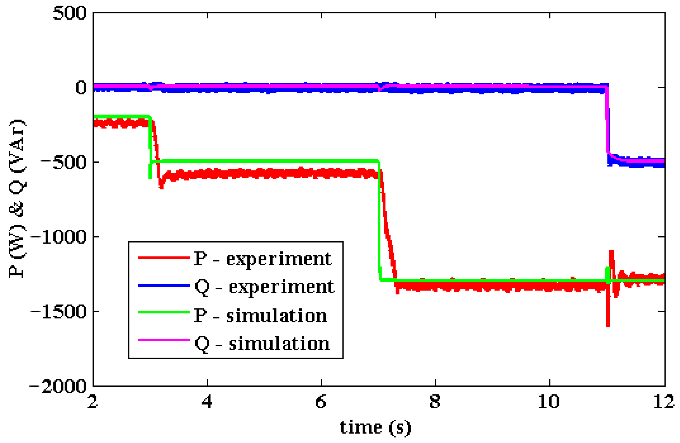
4.4. Verification 4: GSC1 Connected to GSC2 and WFC
The objective of this verification step was to demonstrate the power transfer capability of the MTDC systems. The following step changes were applied:
- Step change in wind turbine torque reference, T3*, from 7 Nm to 12.8 Nm at t = 3 s;
- Step change in GSC2 active power reference, P2*, from 100 W to 900 W at t = 7 s;
- Step change in GSC2 reactive power reference, Q3*, from 0 VAr to −500 VAr at t = 11 s.
The resulting Vdc response is shown in Figure 12, where the system tries to maintain the 250 V reference despite the above step changes. Further, the active power flow control and the reactive power flow control operations are shown in the upper and lower sections of Figure 13, respectively.
As can be observed in Figure 12, the experimental and simulated results are in agreement in terms of reactions to the transients caused by the step changes in the reference inputs. However, the experimental transient responses are slower and show less overshoot, while the simulated ones are faster with higher overshoots.
In Figure 13, it can be observed that the reactive power Q3 follows the reference with some insignificant dq cross-coupling in both the experimental and simulation results. The active power P2 also follows its reference, although with some DC shifts at lower power levels, which may be due to unmodeled non-linearities.
4.5. Discussion
Generally, in all control verifications considered in this study, the hardware verifications showed slower responses compared to their simulation model counterparts. The possible reasons for this could have been that linear models were used as the simulation models, while the actual systems may have contained unmodeled non-linearities. In addition, cross-coupling was observed between the DC link voltage control loop and the reactive power control loop in GSC1, between the active and reactive power control loops in GSC2, and between the frequency control loop and reactive power control loop in WFC, which is why there were disturbances on one loop when the reference on the other loop was changed. This may be treated using line resistance corrections in the controller implementations.
5. Conclusions
The mathematical modeling of an offshore wind farm integrated with a cross-country HVDC network, i.e., MTDC network, has been presented along with simulation results relating to the dynamic behavior and backed up by experimental verifications.
The dynamic behavior results for the GSC1 system equipped with DC link voltage control and reactive power control agreed with the simulation results for the mathematical modeling. Similarly, the experimental results for the dynamic behavior of GSC1 and GSC2 connected configurations, with the latter equipped with active and reactive power control, matched the results obtained in the simulation. In addition, for the same scenario with the WFC equipped with frequency and reactive power control, forming the full MTDC, the dynamic behavior obtained from the hardware experiment and the simulation results agreed.
Despite the unmodeled nonlinearities and mild cross-coupling between control loops, the modeling tools followed the actual behavior of the MTDC under both dynamic and steady-state conditions. Hence, it was concluded that the developed tools can be used to conduct dynamic studies of cross-country MTDCs.
Author Contributions
Conceptualization, L.S., C.E.U.-L., J.B.E. and O.D.A.; methodology, L.S. and C.E.U.-L.; software, L.S. and O.D.A.; validation, L.S. and O.D.A.; formal analysis, L.S., C.E.U.-L., J.B.E. and J.L.; investigation, L.S. and J.B.E.; resources, C.E.U.-L., J.B.E. and O.D.A.; data curation, L.S. and O.D.A.; writing—original draft preparation, L.S., C.E.U.-L., J.B.E. and O.D.A.; writing—review and editing, J.L.; visualization, L.S., C.E.U.-L. and O.D.A.; supervision, J.B.E.; project administration, J.B.E. All authors have read and agreed to the published version of the manuscript.
Funding
This research received no external funding.
Institutional Review Board Statement
Not applicable.
Informed Consent Statement
Not applicable.
Data Availability Statement
The data used and generated in this study will be made available on demand.
Conflicts of Interest
The authors declare no conflict of interest.
References
- Ullah, N.; Sami, I.; Chowdhury, M.S.; Techato, K.; Alkhammash, H.I. Artificial Intelligence Integrated Fractional Order Control of Doubly Fed Induction Generator-Based Wind Energy System. IEEE Access 2021, 9, 5734–5748. [Google Scholar] [CrossRef]
- Almutairi, K.; Mostafaeipour, A.; Jahanshahi, E.; Jooyandeh, E.; Himri, Y.; Jahangiri, M.; Issakhov, A.; Chowdhury, S.; Hosseini Dehshiri, S.J.; Hosseini Dehshiri, S.S.; et al. Ranking Locations for Hydrogen Production Using Hybrid Wind-Solar: A Case Study. Sustainability 2021, 13, 4524. [Google Scholar] [CrossRef]
- Chowdhury, M.S.; Rahman, K.S.; Selvanathan, V.; Nuthammachot, N.; Suklueng, M.; Mostafaeipour, A.; Habib, A.; Akhtaruzzaman, M.; Amin, N.; Techato, K. Current trends and prospects of tidal energy technology. Environ. Dev. Sustain. 2021, 23, 8179–8194. [Google Scholar] [CrossRef] [PubMed]
- Stern, N. Stern Review: The Economics of Climate Change. 2006. Available online: http://mudancasclimaticas.cptec.inpe.br/~rmclima/pdfs/destaques/sternreview_report_complete.pdf (accessed on 20 October 2021).
- World Energy Council. World Energy Trilemma. In Time to Get Real—The Case for Sustainable Energy Investment; World Energy Council: London, UK, 2013. [Google Scholar]
- Ryndzionek, R.; Sienkiewicz, Ł. Evolution of the HVDC Link Connecting Offshore Wind Farms to Onshore Power Systems. Energies 2020, 13, 1914. [Google Scholar] [CrossRef] [Green Version]
- Pecoraro, G.; Pascucci, A.; Carlini, E.M.; Contu, M.; Cortese, M.; Gnudi, R.; Allella, F.; Bruno, G.; Michi, L. HVDC link between Italy and Montenegro: Impact of the commissioning on the real-time operation. In Proceedings of the 2019 AEIT International Annual Conference (AEIT), Florence, Italy, 18–20 September 2019; pp. 1–6. [Google Scholar] [CrossRef]
- Iaria, A.; Rapizza, M.R.; Marzinotto, M. Control functions for a radially operated three-terminal VSC-HVDC system: The SA.CO.I. HVDC case. In Proceedings of the 2018 IEEE International Conference on Industrial Technology (ICIT), Lyon, France, 20–22 February 2018; pp. 1679–1684. [Google Scholar] [CrossRef]
- Giorgi, A.; Rendina, R.; Georgantzis, G.; Marchiori, C.; Pazienza, G.; Corsi, S.; Pincella, C.; Pozzi, M.; Danielsson, K.G.; Jonasson, H.; et al. The Italy-Greece HVDC Link. Cigré Session. 2002. Available online: https://library.e.abb.com/public/a759b260ee9d2d78c1256fda004aeab3/THE%20ITALY-GREECE%20HVDC%20LINK%20.pdf (accessed on 20 October 2021).
- Andersen, B.R. HVDC transmission-opportunities and challenges. In Proceedings of the 8th IEE International Conference on AC and DC Power Transmission (ACDC 2006), London, UK, 28–31 March 2006; pp. 24–29. [Google Scholar]
- Bahrman, M.P. HVDC transmission overview. In Proceedings of the 2008 IEEE/PES Transmission and Distribution Conference and Exposition, Chicago, IL, USA, 21–24 April 2008; pp. 1–7. [Google Scholar]
- European Offshore Supergrid Proposal, Airtricity. Available online: airtricity_supergrid_V1.4.pdf (accessed on 12 October 2021).
- Veum, K. Roadmap to the Deployment of Offshore Wind Energy in the Central and Southern North Sea (2020–2030); ECN: Petten, The Netherlands, 2011. [Google Scholar]
- Durakovic, A. European TSOs Form Eurobar to Standardise Offshore Grids. 15 April 2021. Available online: https://www.offshorewind.biz/2021/04/15/european-tsos-form-eurobar-to-standardise-offshore-grids/ (accessed on 20 October 2021).
- Ye, Y.; Qiao, Y.; Xie, L.; Lu, Z. A Comprehensive Power Flow Approach for Multi-terminal VSC-HVDC System Considering Cross-regional Primary Frequency Responses. J. Mod. Power Syst. Clean Energy 2020, 8, 238–248. [Google Scholar] [CrossRef]
- Raza, A.; Dianguo, X.; Xunwen, S.; Weixing, L.; Williams, B.W. A Novel Multiterminal VSC-HVdc Transmission Topology for Offshore Wind Farms. IEEE Trans. Ind. Appl. 2017, 53, 1316–1325. [Google Scholar] [CrossRef]
- Torbaghan, S.S.; Gibescu, M.; Rawn, B.G.; Van der Meijden, M. A Market-Based Transmission Planning for HVDC Grid—Case Study of the North Sea. IEEE Trans. Power Syst. 2014, 30, 784–794. [Google Scholar] [CrossRef] [Green Version]
- Rodrigues, S.; Pinto, R.T.; Bauer, P.; Pierik, J. Optimal Power Flow Control of VSC-Based Multi-terminal DC Network for Offshore Wind Integration in the North Sea. IEEE J. Emerg. Sel. Top. Power Electron. 2013, 1, 260–268. [Google Scholar] [CrossRef]
- ABB. XLPE Submarine Cable Systems Attachment to XLPE Land Cable Systems—User’s Guide. Available online: https://new.abb.com/docs/default-source/ewea-doc/xlpe-submarine-cable-systems-2gm5007.pdf (accessed on 20 October 2021).
- Su, M.; Dong, H.; Chen, X.; Liu, K. Modeling and Analysis of VSC-MTDC Transmission Systems. In Proceedings of the 2019 IEEE Innovative Smart Grid Technologies—Asia (ISGT Asia), Chengdu, China, 21–25 May 2019; pp. 445–450. [Google Scholar] [CrossRef]
- Sayed, S.; Massoud, A. A Matlab/Simulink-Based Average-Value Model of Multi-Terminal HVDC Network. In Proceedings of the 2019 2nd International Conference on Smart Grid and Renewable Energy (SGRE), Doha, Qatar, 19–21 November 2019; pp. 1–6. [Google Scholar] [CrossRef]
- Zou, W.; Dong, H.; Chen, X.; Liu, K. Small Signal Modeling and Decoupling Control of VSC-MTDC. In Proceedings of the 2020 Chinese Control and Decision Conference (CCDC), Hefei, China, 22–24 August 2020; pp. 2786–2792. [Google Scholar] [CrossRef]
- De Decker, J. An offshore transmission grid for wind power integration: The European techno-economic study OffshoreGrid. In Proceedings of the IEEE PES General Meeting, Minneapolis, MN, USA, 25–29 July 2010; pp. 1–8. [Google Scholar]
- Ugalde-Loo, C.E.; Liang, J.; Ekanayake, J.; Jenkins, N. State-Space Modelling of Variable-Speed Wind Turbines for Power System Studies. IEEE Trans. Ind. Appl. Soc. 2013, 49, 223–231. [Google Scholar] [CrossRef]
- Castro, L.M.; Acha, E. A Unified Modeling Approach of Multi-Terminal VSC-HVDC Links for Dynamic Simulations of Large-Scale Power Systems. IEEE Trans. Power Syst. 2016, 31, 5051–5060. [Google Scholar] [CrossRef]
- Pinares, G.; Tjernberg, L.B.; Tuan, L.A.; Breitholtz, C.; Edris, A.A. On the analysis of the dc dynamics of multi-terminal VSC-HVDC systems using small signal modelling. In Proceedings of the 2013 IEEE Grenoble Conference, Grenoble, France, 16–20 June 2013; pp. 1–6. [Google Scholar] [CrossRef] [Green Version]
- Adam, G.P.; Ahmed, K.H.; Finney, S.J.; Williams, B.W. Generalized modeling of DC grid for stability studies. In Proceedings of the 4th International Conference on Power Engineering, Energy and Electrical Drives, Istanbul, Turkey, 13–17 May 2013; pp. 1168–1174. [Google Scholar] [CrossRef]
Figure 1.
Block diagram of the wind farm, transmission line, and AC-to-DC converter.

Figure 2.
Grid-connected converter with DC link voltage control and reactive power control.

Figure 3.
Grid-connected converter with active power control and reactive power control.

Figure 4.
Overall system block diagram for the MTDC network.

Figure 5.
Hardware-in-the-loop experimental platform: (a) VSC-MTDC test rig and dSPACETM graphical user interface; (b) power amplifier (left) interfacing the MTDC test rig and the RTDS (right); (c) 10 kW PMSGs in the WFG.
Figure 5.
Hardware-in-the-loop experimental platform: (a) VSC-MTDC test rig and dSPACETM graphical user interface; (b) power amplifier (left) interfacing the MTDC test rig and the RTDS (right); (c) 10 kW PMSGs in the WFG.

Figure 6.
Reactive power and DC link voltage control schemes for GSC1.

Figure 7.
Active and reactive power control schemes for GSC2.

Figure 8.
Frequency and reactive power control for WFC.

Figure 9.
Comparison of experimental and simulation step responses in DC link voltage and reactive power flow for GSC1 only.
Figure 9.
Comparison of experimental and simulation step responses in DC link voltage and reactive power flow for GSC1 only.

Figure 10.
Comparison of experimental and simulation step responses in active power flow and reactive power flow for GSC1 connected to GSC2.
Figure 10.
Comparison of experimental and simulation step responses in active power flow and reactive power flow for GSC1 connected to GSC2.

Figure 11.
Comparison of experimental and simulation step responses in wind farm frequency and reactive power flow for GSC1 connected to WFC.
Figure 11.
Comparison of experimental and simulation step responses in wind farm frequency and reactive power flow for GSC1 connected to WFC.

Figure 12.
Comparison of experimental and simulation results in terms of DC link voltage for GSC1 connected to GSC2 and WFC.
Figure 12.
Comparison of experimental and simulation results in terms of DC link voltage for GSC1 connected to GSC2 and WFC.

Figure 13.
Comparison of experimental and simulation step responses in active power flow and reactive power flow for GSC1 connected to GSC2 and WFC.
Figure 13.
Comparison of experimental and simulation step responses in active power flow and reactive power flow for GSC1 connected to GSC2 and WFC.


Table 1.
Definitions of symbols used in Figure 1.
Table 1.
Definitions of symbols used in Figure 1.
| Symbol | Definition |
|---|---|
| Vdw, Vqw | dq voltages of the AC side of the converter; |
| Vd, Vq | dq voltages of the generator output; |
| Id, Iq | dq currents on the AC side of the converter; |
| Ld, Lq | dq axis inductances of the PMSG; |
| R | winding resistance of the PMSG; |
| λpm | flux linkage of the PMSG; |
| ωw | electrical speed of the PMSG; |
| rotor speed of the PMSG; | |
| number of pole pairs of the PMSG; | |
| Lw | transmission line inductance; |
| τ | induced torque; |
| τm | mechanical torque given by the turbine; |
| DC voltage of the converter; | |
| reference DC voltage of the converter; | |
| d and q modulation indexes of the converter; |
Table 2.
Definitions of symbols used in Figure 2.
Table 2.
Definitions of symbols used in Figure 2.
| Symbol | Definition |
|---|---|
| Vd1, Vq1 | dq voltages of converter AC side; |
| Vgd1,Vgq1 | dq voltages of grid; 1 |
| Id1, Iq1 | dq currents of the AC side of the converter; |
| R1 | transmission line resistance; |
| L1 | transmission line inductance; |
| grid 1 frequency in rad/s; | |
| DC voltage of the converter; | |
| reference DC voltage of the converter; | |
| dq modulation indexes of the converter. |
Publisher’s Note: MDPI stays neutral with regard to jurisdictional claims in published maps and institutional affiliations. |
© 2022 by the authors. Licensee MDPI, Basel, Switzerland. This article is an open access article distributed under the terms and conditions of the Creative Commons Attribution (CC BY) license (https://creativecommons.org/licenses/by/4.0/).
Share and Cite
MDPI and ACS Style
Samaranayake, L.; Ugalde-Loo, C.E.; Adeuyi, O.D.; Licari, J.; Ekanayake, J.B. Multi-Terminal DC Grid with Wind Power Injection. Wind 2022, 2, 17-36. https://doi.org/10.3390/wind2010002
AMA Style
Samaranayake L, Ugalde-Loo CE, Adeuyi OD, Licari J, Ekanayake JB. Multi-Terminal DC Grid with Wind Power Injection. Wind. 2022; 2(1):17-36. https://doi.org/10.3390/wind2010002
Chicago/Turabian StyleSamaranayake, Lilantha, Carlos E. Ugalde-Loo, Oluwole D. Adeuyi, John Licari, and Janaka B. Ekanayake. 2022. "Multi-Terminal DC Grid with Wind Power Injection" Wind 2, no. 1: 17-36. https://doi.org/10.3390/wind2010002