Article

A Novel Algorithm for Controlling Active and Reactive Power Flows of Electric Vehicles in Buildings and Its Impact on the Distribution Network

1
Department of Electrical Engineering, Concordia University, Montreal, QC H3G 1M8, Canada
2
Department of Electrical Engineering, Ecole de Technologie Superieure, Montreal, QC H3C 1K3, Canada
3
Mechanical Engineering Department, McGill University, Montreal, QC H3A 0G4, Canada
4
Department of Electrical Engineering, Faculty of Technology, University of Batna 2, Fesdis 05078, Batna, Algeria
*
Author to whom correspondence should be addressed.
World Electr. Veh. J. 2020, 11(2), 43; https://doi.org/10.3390/wevj11020043
Submission received: 10 February 2020 / Revised: 25 May 2020 / Accepted: 29 May 2020 / Published: 30 May 2020

Abstract

:
In the literature, many optimization algorithms were developed to control electrical loads, especially Electric Vehicles (EVs) in buildings. Despite the success of the existing algorithms in improving the power profile of charging EVs and reducing the total electricity bill of the end-users, these algorithms didn’t show significant contribution in improving the voltage profile on the network, especially with the existence of highly inductive loads. The control of the active power may not be sufficient to regulate the voltage, even if sophisticated optimization algorithms and control strategies are used. To fill the gap in the literature, we propose a new algorithm that is able to control both the active and reactive power flows using electric vehicles in buildings and homes. The algorithm is composed of two parts; the first part uses optimization to control the active power and minimize the electricity bill, while the second part controls the reactive power using the bidirectional converter in the EV in a way that the voltage profile on the distribution transformer respects its limits. The new approach is validated through a comparative study of four different scenarios, (i) without EV, (ii) with EV using uncoordinated charging, (iii) with EV using coordinated charging, (iv) with EV using our proposed algorithm. Results show that our algorithm has maintained the voltage within the recommended limits, and it has minimized the peak load, the electricity cost, and the techno-economic losses on the network.

Graphical Abstract

1. Introduction

1.1. Problem Statement

Plug-in electric vehicles (EVs) are considered as a promising technology to reduce the consumption of fossil fuel and the emission of CO2 and other harmful gases (SO2, NOx, etc.) [1]. Plug-in hybrid electric vehicles (PHEVs) and fully battery electric vehicles (BEVs) are lumped together in this study by (EVs), in which the vehicles can be connected to the grid. EVs will definitely support the future deployment of smart grids because they are considered as a spinning reserve and able to store and deliver energy whenever it is needed. The integration of EVs has many benefits, such as providing ancillary services to the grid [2,3], and providing stability when fluctuant renewable energy sources are connected to the network [1,4,5]. Despite all the advantages that EVs can provide the smart grid, their integration should be supervised and controlled to maximize the profit from their existence. Hence, extensive studies should be conducted to propose the best optimization algorithms and control strategies that maximize the benefit of integrating EVs into the distribution systems.

1.2. Literature Review

The study of the integration of electric vehicles into the distribution system goes back to the 1980s, when the coordinated charging of EVs was examined and papers published as in [6]. Since then, the integration of EVs has become a hot topic, and scientists started to study how to charge EVs in a way to minimize the negative impact of their charging on the distribution network [7,8,9]. Some papers studied how to control the charging of EVs using unidirectional converters, while others studied the impact of controlling the charging and discharging of EVs on the network using bidirectional converters and charging strategies [10,11,12,13,14,15,16,17,18]. Usually, each charging strategy (uni- or bi-directional) has its advantages and barriers. The bidirectional charging strategies have many more benefits than the other method since they provide more ancillary services even during peak demand periods [2,16,19,20,21]. Such benefits include: voltage regulation [15,22,23], frequency regulation [24], spinning reserve participation [19], supporting the integration of renewable energy sources (RES) [2,5,19,25] etc. It is important to note that uncoordinated charging and discharging strategies do not have a positive impact on the network, even if EVs are introduced in small quantities [26,27]. Therefore, it is always recommended to use coordinated charging strategies, although their implementation implies complexity and higher cost.

1.3. Impediments and Barriers of Other Studies

In recent years, the integration of EVs into buildings becomes an interesting topic to study [28,29,30,31]. Studies used many optimization algorithms and control strategies to get the most from their integration. The mostly used objective function was to minimize the electricity cost at home by optimizing the charging of EVs and other loads [32,33]. Regarding the constraints to be considered for optimal operation, many papers did not consider the active power limit of a distribution transformer ( P t T L ), the active power limit at home level ( P t H L ), and the active power limit of the main circuit breaker at home ( P t H L _ C B ) [25,34]. Exceeding P t T L may result in an overload on the distribution transformer (DT) and may reduce its lifetime and increase the electrical and financial losses [35]. The transformer’s lifetime and its voltage profile are negatively affected even when optimization algorithms are used without considering the limits at homes and the distribution network. Other papers considered the limit on the transformer as constant [23], or variable [36], depending on the internal characteristics of the DT, such as temperature. The problem in these studies is that the proposed limits do not consider the electrical loads that exist on other transformers connected to the network. Hence, the total load demand of all electrical loads may highly affect the stability and create severe voltage drop on certain transformers, especially when high energy-demanding loads such as EVs are connected. Moreover, the reactive power has a much higher impact on the voltage profile compared to the active power. Therefore, a house/building with high consumption of reactive power may worsen the voltage profile drastically, not just on the local transformer, but also it might affect other vulnerable transformers on the network. To make things much clearer, Figure 1 shows two different cases for the same electrical network. Transformer 1 is supplying 2 other transformers (2 and 3). Each transformer is feeding a certain number of houses or buildings. In the first scenario, homes are considered without connecting EVs, while in the second case, and on the second transformer “2”, EVs are plugged-in at homes. On the right side of the figure, there are some voltage profiles that represent how the voltage varies in time on each transformer. The first two voltage profiles in case 1 respect the minimum and maximum limits (a minimum of 0.95, and a maximum of 1.05 per unit [pu]). In this example, everything seems to be all right before connecting EVs. In the second case, when EVs are connected to the second transformer, there might not be a severe voltage deviation on the transformer. However, the increasing demand for “transformer 2” due to EVs may affect the voltage profile on the transformer 3 even if its total load demand did not change. Moreover, homes on transformer 3 are not supposed to reduce their load demands because the power consumption did not change, and homes on transformer 2 will not reduce their power demand because the voltage profile on the transformer respects the limits. What will be the solution in this case? Which customer is responsible for the voltage deviation on transformer 3? This problem was not addressed in previous papers to the best of the authors’ knowledge.
In order to avoid such problems, in this paper, both active and reactive power are considered in order to reduce the voltage deviation on the DTs and minimize the electrical and economic losses on the network. The regulation of the reactive power flow from EVs has a better impact on improving the voltage profile than the active power flow, which will be demonstrated in this paper. Hence, in the previous example, homes on the second transformer can use the bidirectional converters to inject reactive power to the grid in order to improve the voltage profile on their transformer and on the transformer of their neighbors, as presented in Figure 2.

1.4. Contributions

The contribution of this paper is presented in the development of a novel algorithm that is able to optimize and control the active and reactive power flow of the EVs at homes and buildings. The proposed algorithm minimizes the electricity cost at home or building, respects the active, reactive power and voltage limits on the distribution transformer, reduces the techno-economic losses on the network even under different pricing mechanisms (such as a Fixed price, Time-of-Use and Real-Time price). In addition, the algorithm considers the following:
  • Main and branch circuit breaker rating into the optimization model,
  • Upper and lower limits of both active and reactive power on the distribution transformer,
  • real charging and discharging power profiles of the EVs,
  • It predicts and calculates the available power to be consumed at each instant and inform the end-user how much energy is left to use every day to charge his EV while respecting the power and energy limits at home,
  • It informs the end-user how much energy he should reduce at home in order to attain the desired State of Charge level,
  • The discharging mode could be selected according to the EV owner’s desire,
  • The algorithm gives the EV owner the choice to participate or not in the ancillary services such as voltage and power flow regulations.
The study is realized for a single EV at home, and then it is generalized to a large area of homes supplied by the same transformer. The EVs penetration level is 100%, which means that every home has its own EV. A comparative study between four different scenarios is presented in order to validate the suggested algorithm: (a) a home without EV; (b) a home with EV using uncoordinated charging; (c) a home with EV using coordinated charging; (d) and home with EV using our proposed algorithm to charge and discharge the EV.

1.5. Paper Organization

Section 2 presents the problem formulation. Results and discussions for a single home are shown in Section 3. In Section 4, the study is generalized to a cluster of homes supplied by the same bus using IEEE (Institute of Electrical and Electronic Engineering) 13 node test feeder as standard. Section 5 shows a summary of the main outcomes of the proposed algorithm. Section 6 presents the conclusion and future work. Finally, the nomenclature is given.

2. Problem Formulation

The problem formulation consists of introducing both active and reactive power in the optimization model and the algorithm. Static, dynamic, and discrete constraints related to the EV, the owner, the power and energy demand, the transformer capacity, and the grid are considered in order to guarantee an optimal solution.

2.1. Objective Function

The objective of the optimization is to minimize the electricity cost at home by controlling the charging and discharging of the EV as in Equation (1), where T is the period of time for the study; t A is the arrival time when the EV at home is plugged-in; Δ t is the time step interval. P L o a d ( t ) is the baseload power demand of the home without the presence of the EV;   C E l e c ( t ) is the cost of electricity at instant “ t ” ($/kWh); S C ( t ) and S D C ( t ) are respectively the binary flags of the charging, and discharging modes (“1” means the mode is turned on; otherwise it is “0”, and just one mode at a time could be applied) [19]; P C ( t ) and P D C ( t ) are the absorbed and injected active power by the EV using charging and discharging modes, respectively.
M i n i m i z e   t = t A t A + T Δ t ( C E l e c ( t ) · ( P L o a d ( t ) + S C ( t ) · P C ( t ) S D C ( t ) ·   P D C ( t ) ) · Δ t )

2.2. Constraints

2.2.1. Mode of Operation

The EV battery status has one among three modes of operations represented by binary variables in Equation (2):
S C ( t ) + S D C ( t ) + S I ( t ) = 1
where, S C ( t ) , S D C ( t ) and S I ( t ) are respectively the binary flags of the charging, discharging, and idle modes (“1” means the mode is turned on; otherwise, it is “0”, and just one mode at a time could be applied) [19]. The defined charging and discharging mode flags in (2) are proposed in this paper as in (3) and (4). They provide a safe functionality of the connected EV.
S C ( t ) = S P l u g ( t ) · S g ( t ) · S A ( t )
S D C ( t ) = S P l u g ( t ) · S l ( t ) · S A ( t )
where, S P l u g ( t ) is the plug status of the EV, it is equal to “1” if the vehicle is connected to the grid, and “0” otherwise; S A ( k ) is the algorithm decision result, it is equal to 1 if the decision is about performing charging or discharging, and 0 if no action should be performed. It is controlled by the arrival and departure time of the EV at home. S l ( t ) = 1 if R U L P ( t ) P L o a d ( t ) < 0 , and “0” otherwise. S g ( t ) = 1 if R U L P ( t ) P L o a d ( t ) > 0 , and “0” otherwise.

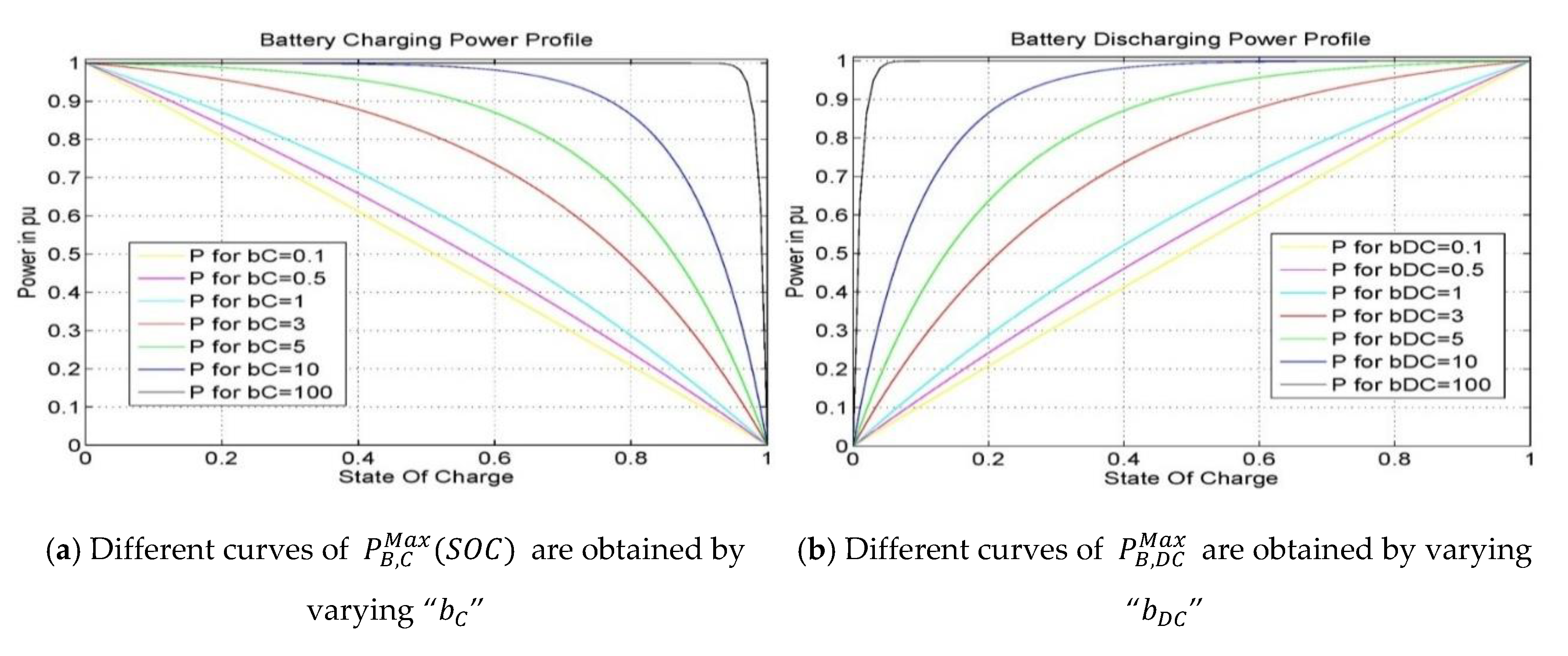
2.2.2. Active Power Constraints

A total load of active power is obtained from (5), where,   P C ( t ) and P D C ( t ) are the absorbed and injected active power by the EV using charging and discharging modes.
P T o t a l ( t ) = P L o a d ( t ) + S C ( t ) · P C ( t ) S D C ( t ) ·   P D C ( t )
The power limits not to be exceeded on the home’s main circuit breaker (MCB) and on the EV branch circuit breaker (BCB) are proposed in this paper as in (6) and (7), respectively. Respecting these limits avoids the voltage deviation and tripping of the circuit breakers. If these limits are not considered, the total power may exceed the limits and may create lots of problems at home and on the bus.
R U L P ( t ) = V · ( C B N R · α M C B ( t ) ) M C B   c u r r e n t · cos ( φ ( t ) )
P B C B R L ( t ) = V · ( C B N R P E V · α B C B ( t ) ) B C B   c u r r e n t · cos ( φ ( t ) )
where V is the nominal voltage; C B N R and C B N R P E V are the main and branch circuit breaker nominal rates;   φ ( t ) is the phase angle; α M C B ( t ) and α B C B ( t ) are the avoiding tripping factors of the circuit breakers. They are affected by internal factors such as temperature, and age. α M C B ( t ) takes a dynamic value that could change during the time in order to limit the active power absorption, it is controlled by the distribution system operator (DSO), and it helps in the participation of the ancillary services and voltage regulation.
The maximum available active power at home at instant “ t ” is proposed in this paper and described in (8), which could be used by the EV to charge its battery. If this limit is not considered, the total power may exceed the limits.
P A M a x ( t ) = R U L P ( t ) P L o a d ( t )
The respected upper and lower limits of active power at instant “ t ” for the total load, including the EV are proposed in this paper as in (9):
R L L P ( t ) P T o t a l ( t ) R U L P ( t )
where R L L P ( t ) is set to zero. P L o a d ( t ) should be less than R U L P ( t ) otherwise, the discharging mode is activated.
Most of the existing studies consider constant charging and discharging power profiles in the optimization model, which may reduce the accuracy in the results, especially because they are highly non-linear equations. To improve the accuracy in the simulation, we suggest using non-linear power profiles for both charging and discharging processes, as suggested in [37]; these non-linear profiles were applied, and their accuracies were demonstrated in [28,38,39,40]. The maximum charging and discharging power limits for a certain state of charge (SOC) of the battery are considered in this paper as in (10) and (11), respectively. These limits protect the battery from high charging and discharging power rates. Therefore, they protect the battery from overheating and increase their lifetime. The mathematical models are developed to describe charging and discharging power rates for different EVs, as in [41] and [42]. Various mathematical models could be applied for different types of EVs, but the main idea in this study is to introduce these expressions in the optimization models. Where, P B , C M a x ( t ) and P B , D C M a x ( t ) depend on the SOC of the battery [42]; P B , C L and P B , D C L are respectively the maximum allowed power limits to charge and discharge the EV’s battery, they are defined by the manufacturer. These constraints protect the battery from overheating, overcharging, and reducing its life loss. b C and b D C are the charging and discharging rate factors which determine the curve form of P B , C M a x ( t ) and P B , D C M a x ( t ) respectively. S O C M a x is the maximum SOC of the EV battery.
0 P B , C M a x ( t ) P B , C L · ( e b C · S O C ( t ) + e b C · S O C M a x e b C · ( S O C M a x ) 1 )
0 P B , D C M a x ( t ) P B , D C L · ( e b D C · ( 1 S O C ( t ) ) + e b D C · S O C M a x e b D C · ( S O C M a x ) 1 )
The maximum charging and discharging power profile limits described in Equations (10) and (11) are depicted in Figure 3. It can be seen that the profiles are highly non-linear and can affect the results whenever they are considered constants.
The maximum SOC for charging and discharging power which is proposed in this paper as in (12) and (13) respectively, guarantee that the battery energy will never overpass the desired final energy ( B C · S O C D F ) and will never be lower than ( B C · S O C M i n ). If the user wants to fully charge his battery, he just needs to set S O C D F = 1 :
0 P C S O C ( t ) B C · ( S O C D F S O C ( t ) ) η C · Δ t  
0 P D C S O C ( t ) B C · ( S O C ( t ) S O C M i n ) Δ t  
0 P D C , 2 S O C ( t ) B C · η D C · ( S O C D E ( i ) + S O C D C S O C i ) Δ t  
where, S O C D F is the EV desired final SOC at the end of the charging;   η C is the charging efficiency [25]; S O C D E ( i ) is the SOC of the discharged energy at iteration “ i ”. Equation (14) is introduced to limit the discharged energy. If it is not introduced, the discharging process may not respect the SOC limits.
The EV maximum charging and discharging active power rates are proposed in this paper as in (15) and (16) considering other power limits in this paper. The minimum value is chosen among all the values which determine the charging and discharging power of the EV. If they are not considered, the charging and discharging powers may overpass the recommended limits and create additional problems for the system.
P C M a x ( t ) = m i n ( P A M a x ( t ) ; P B , C M a x ( t ) ; P C h M a x ; P C , P E V M a x ( t ) ; P S , C M a x ; P B C B R L ( t ) ; P C S O C ( t ) )
P D C M a x ( t ) = m i n ( P A M a x ( t ) ; P B , D C M a x ( t ) ; P C h M a x ; P D C , P E V M a x ( t ) ; P S , D C M a x ; P B C B R L ( t ) ; P D C S O C ( t ) · η D C ; P D C , 2 S O C ( t ) · η D C )
where, P C h M a x is the maximum allowed charging or discharging power rate set by the charger; P C , P E V M a x ( t ) and P D C , P E V M a x ( t ) are the maximum charging and discharging power rates set by the EV owner; P S , C M a x and P S , D C M a x are the maximum charging and discharging power rates allowed by standards, there is no standard for the discharging mode up to now; both P S , C M a x and P C , P E V M a x values could be regulated by the algorithm if higher values do not affect the performance of the system, the reason for this is to satisfy the client by attaining a SOC level close to the desired level when the period of charging is short; η D C is the discharging efficiency.
It is not recommended to discharge the EV battery more than the calculated limits for many reasons: (i) energy loss due to the efficiencies of discharging and charging processes; (ii) the battery life would be shortened; (iii) the charging rate may increase over its limit; and (iv) the SOC may not attain the desired level. This minimal overpassing load has to be reached while also searching for an optimal value of a second objective that consists of minimizing the total consumed electricity cost.
The absorbed and injected active power rates by the battery are bounded as in (17) and (18) by dynamic limits varying according to the charging and discharging conditions of operations. In the literature, they are considered constant, while in this paper, they are considered dynamic, which gives a realistic and good functioning of the system.
P C M i n ( t ) P C ( t ) P C M a x ( t )
P D C M i n ( t ) P D C ( t ) P D C M a x ( t )
where, P C M i n ( t ) and P D C M i n ( t ) are usually equal to zero in a normal case, but they could be variable according to the needs on the bus.

2.2.3. State of Charge (SOC) Constraints

Equation (19) represents the cumulative SOC in the battery starting from an initial value S O C ( t A ) = S O C i until instant “t”. starting from an initial value.
S O C ( t ) = j = 1 ( t t A ) / Δ t Δ S O C ( t j · Δ t )  
The predicted available SOC at home is proposed in this paper as in (20). The available energy is the energy value that could be used to charge the EV’s battery for reaching the previously defined objectives without exceeding the predefined limits. If this equation is not calculated, the EV owner may not be able to predict what will be the final SOC of his battery. The battery may not be charged to the desired level, and the discharging process is undefined.
S O C A = 1 B C t = t A S t e p Δ t   t D Δ t [ ( 1 U ( P L o a d ( t ) R U L P ( t ) ) ) · ( R U L P ( t ) P L o a d ( t ) ) · Δ t ]
The discharged SOC ( S O C D E ) should follow Equation (21), where S O C D E ( i = 0 ) = S O C i . The iteration i counts the number of occurred discharging at different instant “ t ”. i = 1 means the first occurred discharging, etc. If this equation is not introduced, the discharging mode may not respect the SOC limits.
S O C D E ( i + 1 ) = S O C D E ( i ) S D C ( t ) · P D C M a x ( t ) · Δ t B C  
Equations (22)–(24) are proposed in this paper. They ensure that the total electrical energy used for discharging the battery ( S O C D C ) should be within upper and lower limits. It is set by the user. Where, S O C i = S O C ( t A ) is the initial SOC of the battery.
0 S O C D C ( S O C A ( S O C D F S O C i ) ) · U ( S O C A ( S O C D F S O C i ) )
S O C D F S O C i S O C D C
0 1 B C t = t A t D Δ t ( P D C M a x ( t ) · Δ t ) S O C D C
The used energy in the battery should be between its minimum and maximum limits as in (25):
B C · S O C M i n B C · S O C i + t = t A t D Δ t ( S C ( t ) · P C ( t ) · η C S D C ( t ) · P D C ( t ) ) · Δ t B C · S O C M a x  
If the EV is in the discharging mode, and the battery’s energy becomes equal to the lower limit, the discharging mode is turned off, and the idle mode is turned on until the energy in the battery becomes greater than the lower limit. If the EV is in the charging mode and the battery’s energy becomes equal to the upper limit, the charging mode is turned off, and the idle mode is turned on until the energy in the battery becomes lower than the upper limit.
At the departure time t D , Equation (26) may guarantee that the battery’s energy is equal to the desired final energy ( B C · S O C D F ). But it could be lower if there is not enough available energy at home.
B C · S O C i + t = t A t D Δ t ( S C ( t ) · P C ( t ) · η C S D C ( t ) ·   P D C ( t ) ) · Δ t B C · S O C D F  

2.2.4. Reactive Power Constraints

All the reactive power equations presented in this subsection are mainly proposed in this paper to regulate the voltage deviation on the power grid and limit the absorption and injection of the reactive power. In the literature, these limits are not considered, which may create problems on the power factor limits if the injected or absorbed quantity of reactive power is not controlled.
Q T o t a l ( t ) = Q L o a d ( t ) + Q A ( t ) Q I ( t )
Q T o t a l ( t ) = S T o t a l ( t ) · sin ( cos 1 ( P T o t a l ( t ) S T o t a l ( t ) ) )
A total load of reactive power is obtained from (27) or (28). Equation (27) is used when the DSO orders the EV charger to inject ( Q I ( t ) ) or absorb ( Q A ( t ) ) reactive power. Equation (28) calculates the total reactive power at home. Both equations give the same result. Where, Q L o a d ( t ) is the reactive power demand of the home without EV; S T o t a l ( t ) is the total apparent power.
The respected upper and lower limits of the reactive power are calculated in (29) and (30):
R L L Q ( t ) = V · I · sin ( c o s 1 ( P F M a x ) )
R U L Q ( t ) = V · I · sin ( c o s 1 ( P F M i n ) )
where,   P F M i n and P F M a x are the minimum and maximum power factor limits (between 0.8 and 1.0 for residential buildings [43]). The reactive power is used to regulate the voltage profile in case the active power is not sufficient to maintain the voltage within the standard values. It is assumed that the charger is able to inject and absorb reactive power between values calculated in (32). These limits are set by the DSO.
The total load reactive power at home, including EV must satisfy (31).
R L L Q ( t ) Q T o t a l ( t ) R U L Q ( t )
The charger is able to inject and absorb reactive power between the minimum and maximum limits as in (32):
Q C h M i n Q C h ( t ) Q C h M a x

2.2.5. Voltage Constraint

Equation (33) defines the voltage at home between the minimum and maximum limits. The voltage on the transformer has to be confined between these limits [23].
V m i n D T V ( t ) V m a x D T  

2.3. Management of Home Power

This paper gives priority to the DSO’s satisfaction in which the discharging occurs, and the charging stops when P T o t a l ( t ) R U L P ( t ) . In a few cases, the available energy at home may not be sufficient to charge the battery to the desired level. Therefore, the EV owner may not be satisfied. In order to satisfy the EV owner, there are two possibilities. The first one is to reduce the base load consumption at home. This could be done by managing the loads using smart systems or by informing the user to turn off some electrical appliances. The second one is to increase the circuit breaker nominal rate. Thus, it increases the R U L P ( t ) limit. In this paper, the problem is solved using the first method. Two original equations are proposed for this purpose, as in (34) and (35). The proposed algorithm predicts the available SOC at home ( S O C A ) and if it is less than S O C D F , it notifies the user how much power he should reduce at home in order to attain S O C D F . In another meaning, it notifies him what appliances he should turn off in order to use the vacant energy to charging his EV battery to the desired level. Equation (34) is the general case when the reduced power at home ( P R ) could vary when the EV is plugged-in, and (35) is a particular case when P R is considered constant during the charging process. These two equations are used in the algorithm but they are not constraints.
t = t A t D Δ t P R ( t ) Δ t B C · ( ( S O C D F S O C i ) S O C A ) · ( 1 U ( S O C A ( S O C D F S O C i ) ) )
P R ( t = t A ) B C ( t D t A ) · ( ( S O C D F S O C i ) S O C A ) · ( 1 U ( S O C A ( S O C D F S O C i ) ) )

2.4. Proposed Algorithm to Solve the Problem

The proposed algorithm is divided into two main parts. The first part is the optimization model in which the algorithm starts to control and manage the active power at home by charging and discharging the EV. The main objective is to minimize the electricity cost at home, respecting the constraints mentioned before. Because some constraints are non-linear, the optimization model is considered as non-linear programming in which we have used the “Mixed-Integer Non-linear Programming” (MINLP) algorithm to solve the equations. MATLAB is used for simulation, and the algorithm used is “fmincon” with an interior-point solver, which is able to solve MINLP problems.
The second part consists of regulating both the active and reactive power flow whenever needed in order to reduce the voltage deviation on the transformer, respect its limit, and provide ancillary services to the distribution network.
Proposed Algorithm:
1
Input Data
2
  Electric Vehicle:
3
    -Charging and discharging efficiency
4
    -State of Charge (SOC): Initial, final, minimum, maximum
5
    -Battery Capacity
6
    -Minimum and maximum acceptable charging and discharging power rate
7
    -Arrival and departure time of the EV
8
    -Battery internal characteristics
9
  Power Network:
10
    -Minimum and maximum voltage limits
11
    -Electricity Price
12
    -Transformer active power rating P t D T   L i m i t
13
  Home:
14
    -Main and branch circuit breaker limits and ratings
15
    -Baseload power demand
16
    -Voltage measurement
17
    -Minimum and Maximum Active Power Limits
18
    -Minimum and Maximum Reactive Power Limits          Equations (29)–(31)
19
Calculate the values of:
20
  Respected Upper Limit of the Active Power             Equation (6)
21
  Active Power Limit for the branch circuit breaker         Equation (7)
22
  Maximum available active power at home at instant “t”       Equation (8)
23
  Minimum Active Power Limit                   Equation (9)
24
  Available energy at home to charge the EV            Equation (20)
25
  While “Available energy at home to charge EV” < “Needed energy to
    charge the EV to the desired SOC level” as in Equations (34) and (35),
26
    Ask the user to reduce the power consumption of some appliances at home
27
  End While
28
  Existing reactive power demand at home               Equations (27) and (28)
29
Optimization Process
30
  Optimize the total load according to the objective function     Equation (1)
31
  Subject to the Constraints                      Equations (36) to (26)
32
  Output of the Optimization
33
    -Charging and Discharging Profile of the EV          Equations (10), (11), (17), (18)
34
    -Status of the charging and discharging mode of the EV     Equations (2)–(4)
35
    -Total Active Power demand at home              Equation (5)
36
    -Final State of Charge of the EV’s battery           Equation (19)
37
Calculation on the transformer level (Active and Reactive power demand)
38
  Do the same steps as before for all homes on the same transformer
39
  Calculate the total active power of all homes on the transformer P t D T   L o a d
40
  Calculate the total reactive power of all homes on the transformer Q t D T   L o a d
41
  If P t D T   L o a d > P t D T   L i m i t ,
42
    Reduce R U L P ( t ) and α M C B ( t ) at homes
43
    Go back to Step 19 and start recalculating all the values
44
  End If    %(steps from 19 to 41 are repeated until P t DT   Load P t DT   Limit )
45
  Measure the voltage on the transformer V t DT
46
  If V t DT < V min DT ,
47
    EVs inject reactive power respecting its maximum and minimum limits as in Equations (31) and (32)
48
    Go back to Step 45 and measure V t DT
49
  End If   %(steps are repeated until V t DT V min DT )
50
  If V t DT > V max DT ,
51
    EVs absorb reactive power respecting its maximum and minimum limits as in Equations (31) and (32)
52
    Go back to Step 45 and measure V t DT
53
  End If   %(steps are repeated until V t DT < V max DT )
54
Repeat the whole procedure for the next time interval t next = t initial + Δ t
End of the Algorithm

3. Results and Discussions for a Single Home

3.1. Different Scenarios Are Studied at Home

This paper studies four different scenarios for a home with a single EV: (i) a home without EV (named BL); (ii) a home with EV using the uncoordinated charging strategy (named U); (iii) a home with EV using coordinated charging (only), (named CC), the discharging mode is deactivated; and (iv) a home with EV using coordinated charging and discharging (named CCD). All these scenarios are studied for 3 different pricing mechanisms: (i) fixed price, (ii) time-of-use, and (iii) dynamic price (Figure 4).

3.2. Considerations for a Single Home

The following values are considered for calculation: C B N R = 40 A , V = 230 V , cos ( φ ) = 0.8 ,   C B N R P E V = 16 A , R U L P ( t ) = 7.36 kW . Nissan Leaf is used as EV and B C = 24 kWh [44]. P S , C M a x = P S , D C M a x = 1.92 kW at home [45], and SAE J1772 Standard. P S , D C M a x is supposed to be equal to 1.92 kW for level 1, 5 kW and 10 kW for level 2 and higher levels respectively.   S O C M i n = 0.2 , η C = η D C = 93 % .

3.3. Results for a Single Home

In this subsection, the previously described algorithm is validated by means of simulations performed for each scenario mentioned before. Validation is performed through a comparative study on the following profiles: (i) the total power, (ii) the EV charging and discharging power rates, (iii) the voltage on the distribution board, (iv) the energy cost, (v) and the power losses.

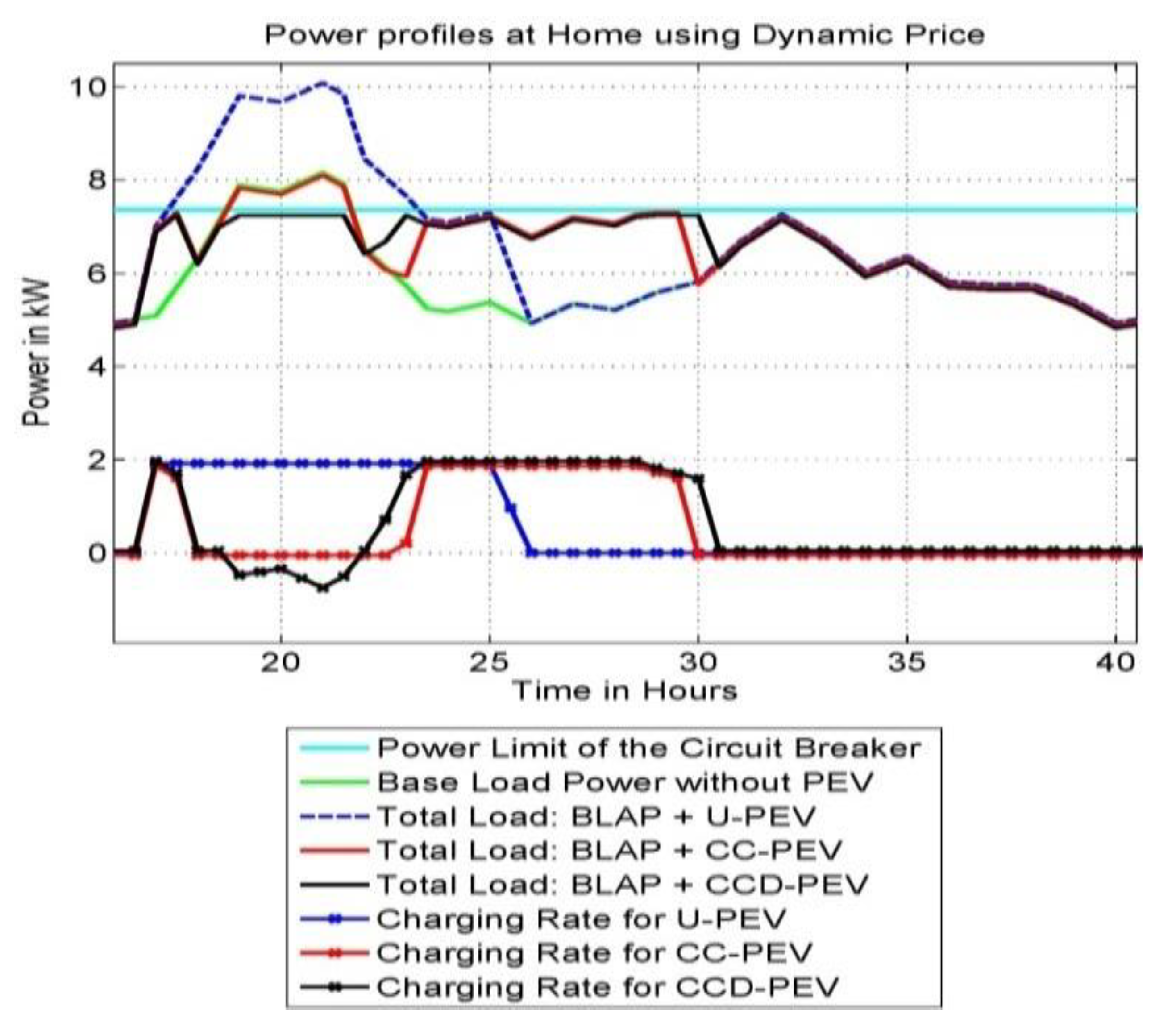
3.3.1. Power and Charging Rates Profiles

The baseload power profile is considered deterministic [46], and according to [34], although a stochastic model is realistic, it will not affect the results significantly. This is assuming, as in Figure 5, RULP is constant.
Results in Figure 5 show that the CCD strategy is the best one, in which the total load respects the limits imposed by the circuit breakers. The EV battery is also charged to the desired level.

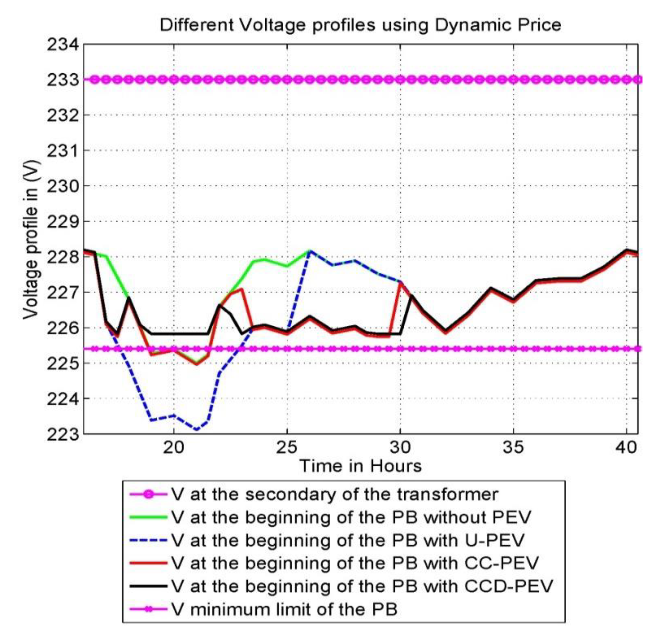
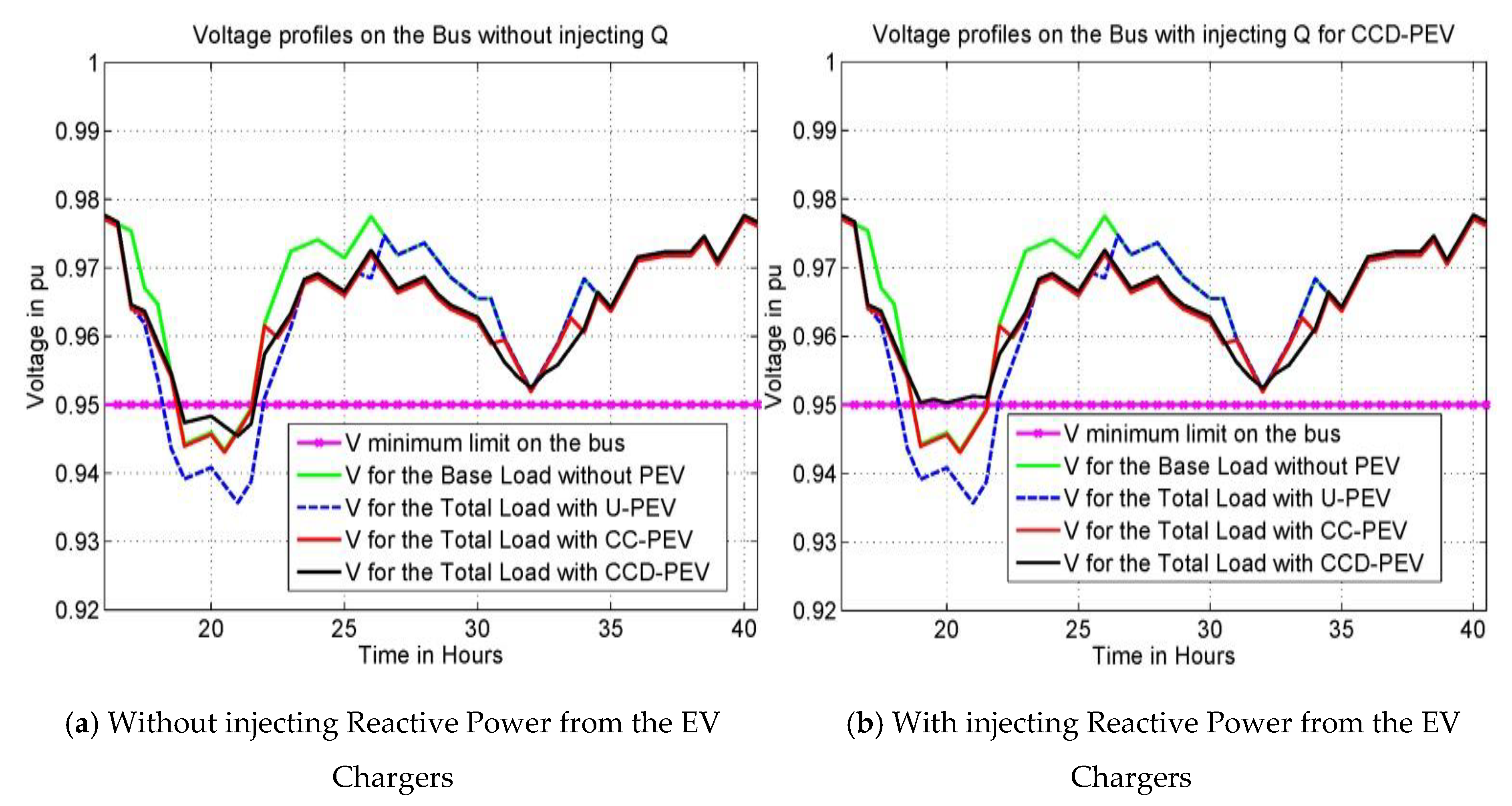
3.3.2. Voltage Profiles

The voltage profiles of the four mentioned scenarios are presented in Figure 6. The results show that the CCD strategy is the best one, in which the voltage profile is maintained within the required limits. Moreover, one has to mention that CCD strategy helps the user to improve the power quality. The installation of capacitor banks or tap transformers is then avoided, and the total cost of the electrical installation is reduced. It is important to mention that the control of the reactive power could be done using only the charger without putting any stress on the battery in order to reduce its life loss.

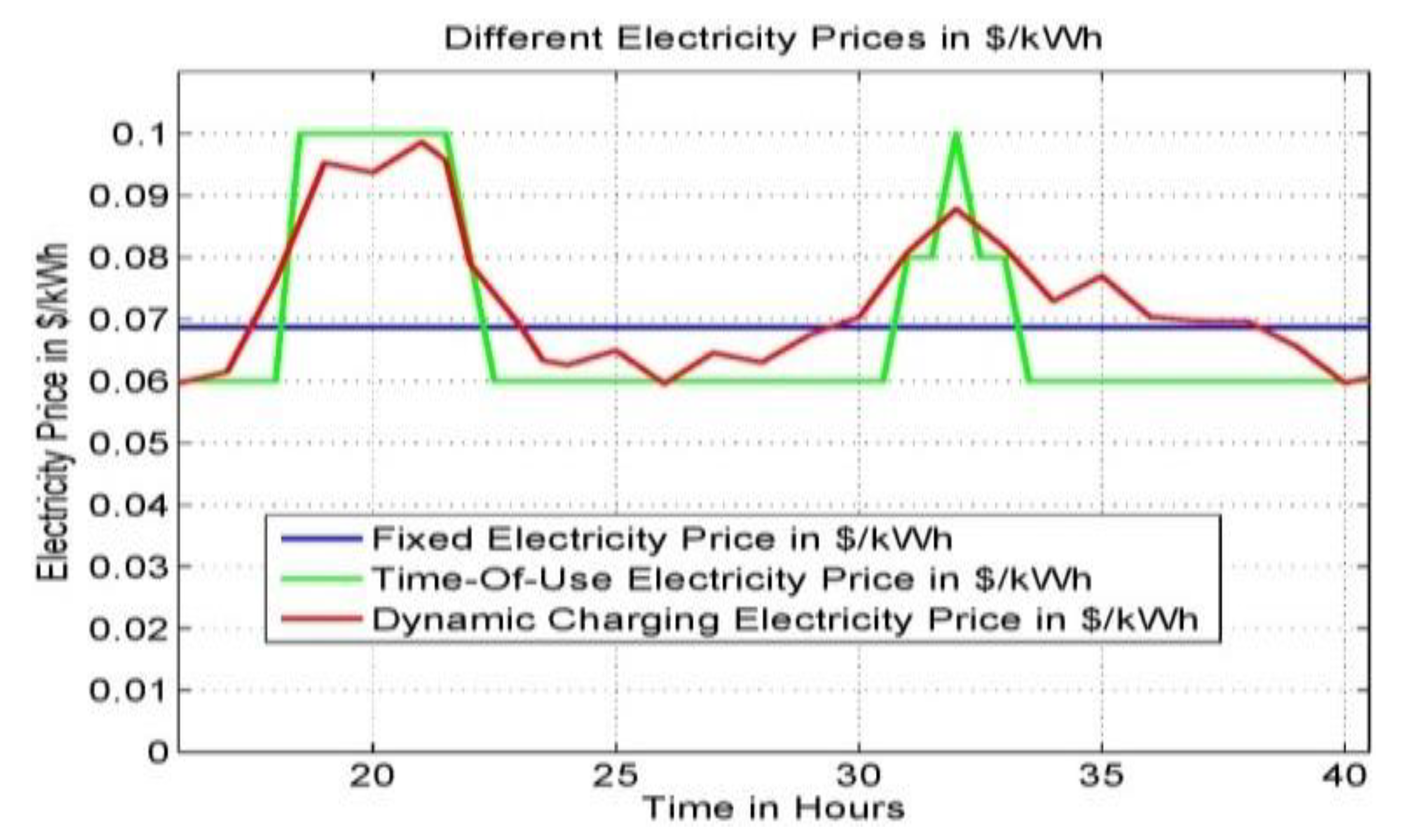
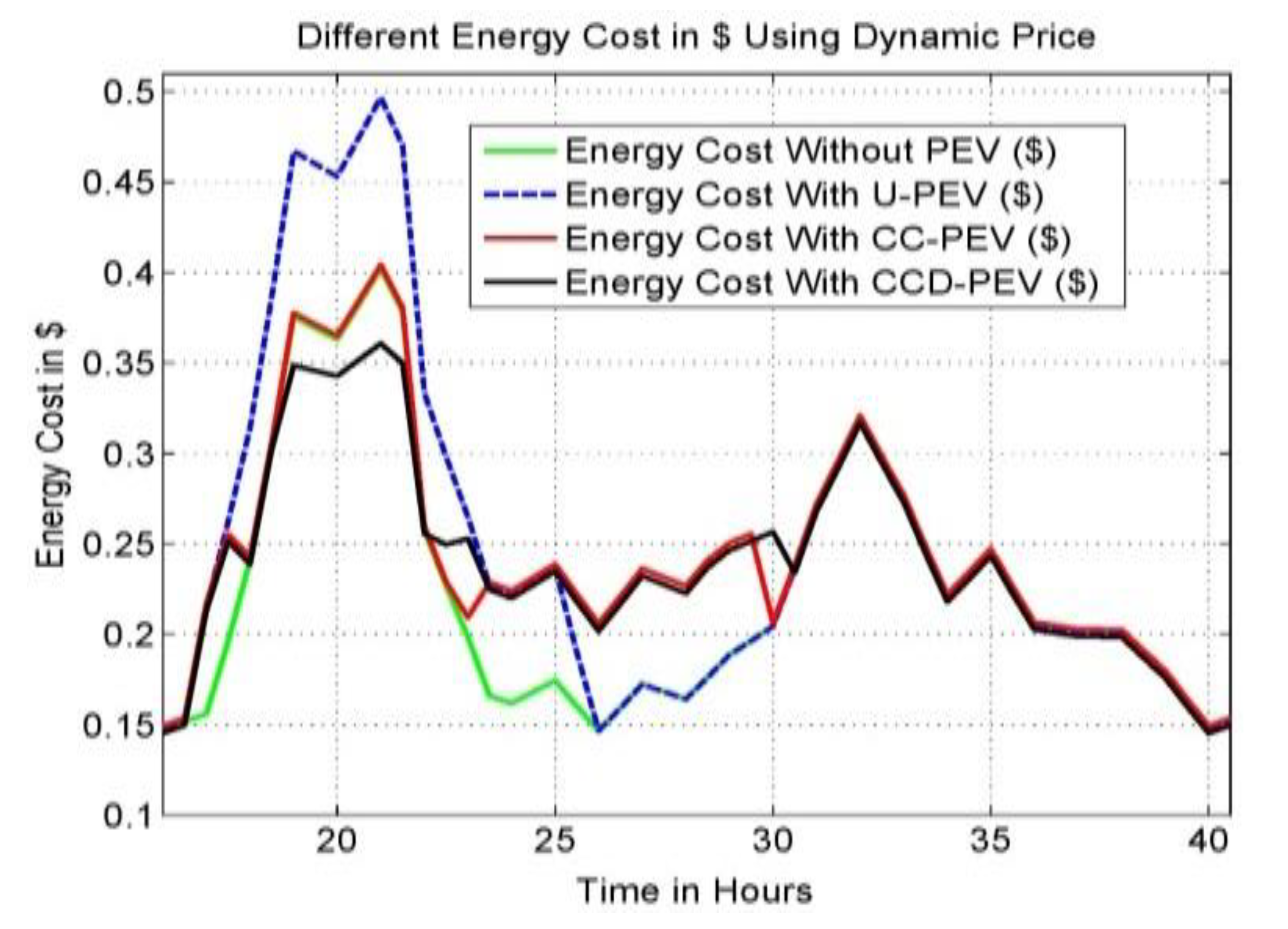
3.3.3. Energy Cost Profiles

The energy cost profiles of the four mentioned scenarios are presented in Figure 7. S O C D F = 0.85 for the CC and CCD strategies, and 1 for the U strategy, while Table 1 represents the study of S O C D F = 1 for the CC, CCD and U strategies.
Table 1 presents a comparison between the four different scenarios stated before. The studies shown are for a dynamic electricity price, and S O C D F = 1 for coordinated charging (CC), coordinated charging and discharging (CCD), and uncoordinated charging (U) strategies. The power loss in percentage is the difference between the total power loss of the Home + EV and the total power loss due to the baseload only. It is obvious that our proposed strategy “CCD-EV” has reduced peak demand compared to other strategies, which becomes 7.36 kW instead of 10.079 kW for the uncoordinated strategy U-EV and 8.159 kW for the coordinated strategy CC-EV. Moreover, it shows that the current value has respected the circuit breaker limit of 40 A, while other strategies have exceeded this limit, 54.777 A for U-EV and 44.342 A for CC-EV. In addition, our proposed strategy CCD-EV has respected the voltage drop within the limit of 2% while other strategies did not, in which the value is 2.993% for U-EV and 2.174% for CC-EV. Regarding the power losses, there are also improvements, in which the losses using our proposed strategy (CCD-EV) are almost 24.8466% while U-EV has a power loss of 28.8594% and the CC-EV also has 24.8875% of power loss compared to the initial case without EV.
It can be concluded from this table that our proposed strategy has improved the performance of the low-voltage electrical network.
Table 2 shows the energy cost at home, including the EV using three different pricing mechanisms represented in Figure 4. The study is done where S O C D F = 1 for U, CC and CCD strategies. It can be seen that all strategies U-EV, CC-EV and CCD-EV have the same electricity cost when a fixed electricity tariff is used as shown in the second row. However, our proposed strategy shows better results when Time-of-Use (TOU) and dynamic pricing are used as shown in the rows 3 and 4. This is due to the fact that our strategy can discharge when the electricity price is high and charge when the electricity price is low in order to minimize the electricity cost at home and maximize the profit from selling electricity to the network.

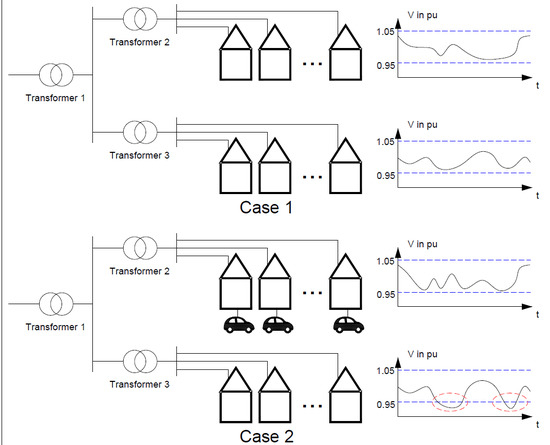
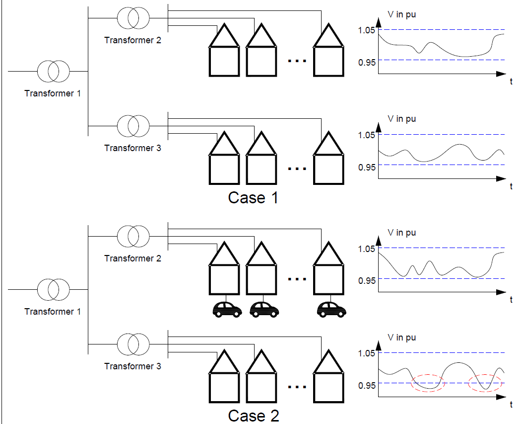
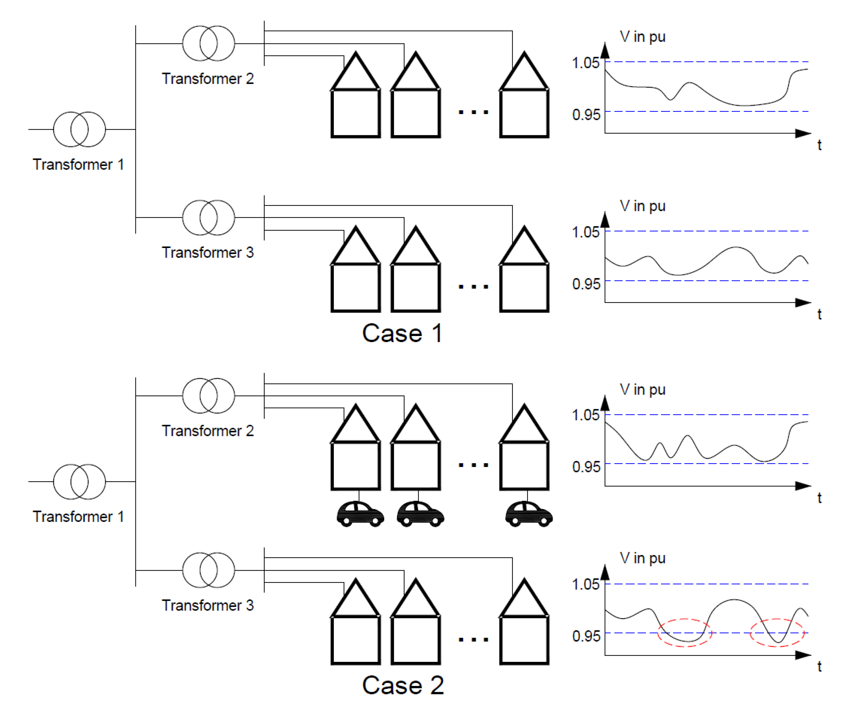
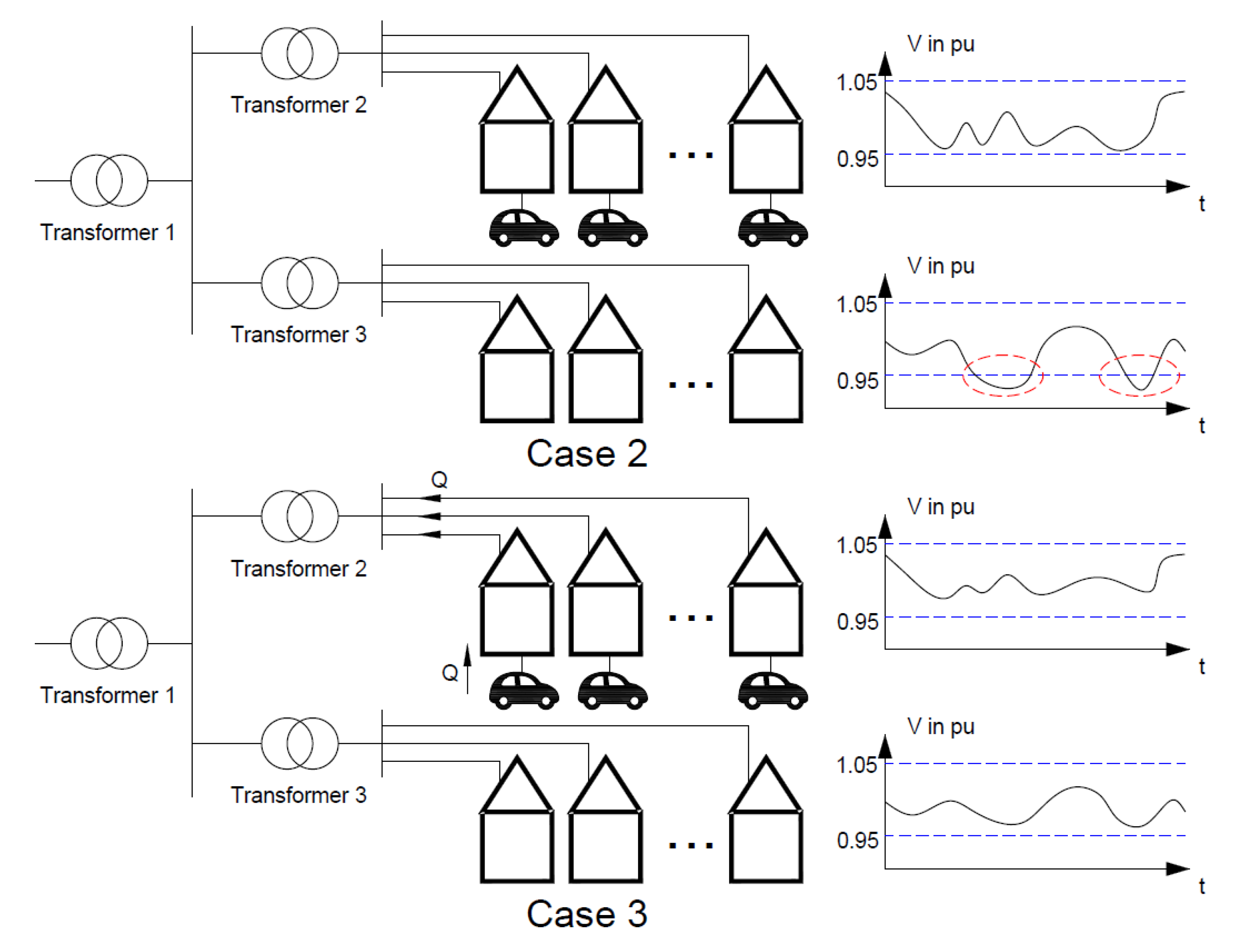
4. Results and Discussions for a Cluster of Homes in the Same Bus

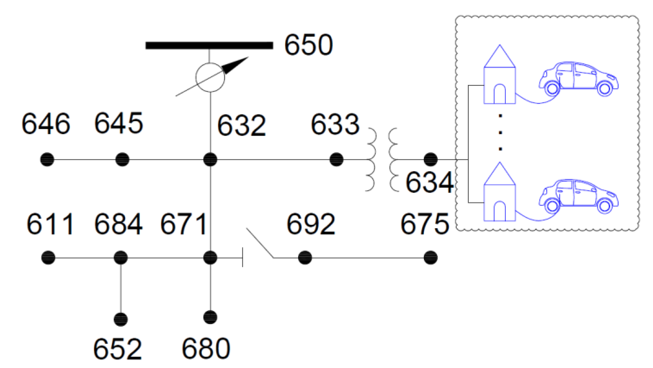
4.1. Considerations for a Cluster of Homes on the Same Bus

The presented study in the previous section is generalized to a larger area of homes on the same bus. The four presented scenarios will be considered in this section in order to see their impact on the bus and on the distribution grid. In this study, the IEEE 13 node distribution test feeder is considered (Figure 8) [47], the simulation is done using OpenDSS and MATLAB. The EV owners and their houses are located on bus 634 in which the penetration level of EVs is equal to 100%, in another meaning, every home has its own EV. Two different studies are undertaken; the first one is when the EVs are able to supply only active power to the grid, and the second one is when the EVs and their chargers are able to supply active and reactive power to the grid, respectively. OpenDSS is software that simulates a distribution network. In this paper, it is used in order to see the impact of the proposed algorithm not just at home levels but on the distribution network also. The software gives detailed results regarding the voltage drop, line and transformer losses, active and reactive power flow, and many others. For the studied case in this paper, we firstly considered a single home, then a cluster of homes on the same bus. The bus is a part of a network. Hence, it is necessary to study the complete network in order to see what will be the impact of different scenarios on the whole system, not just on a single transformer. OpenDSS is a powerful tool that allows the user to do a load flow analysis once it is run. It simulates and calculates the active and reactive power flow, the voltage, the current, and the phasing angle on each element of the system.

4.2. Results for a Cluster of Homes on the Same Bus

Figure 9a,b present the voltage profiles of the total load on the bus for the four mentioned scenarios. In Figure 9a, EVs are used to supply only active power to the grid for the CCD strategy. It can be seen that all strategies have exceeded the voltage limit imposed by the bus during the on-peak period, although active power is injected for the CCD strategy. Moreover, due to the previously mentioned constraints, the injection of the active power cannot exceed the imposed limits. In Figure 9b, the EV chargers at homes have injected a small amount of reactive power to the grid when the CCD strategy is considered. In this case, the voltage profile is improved, and it is confined within the required limits on the bus.

5. Summary of the Main Outcomes of the Proposed Algorithm

To summarize the study, the algorithm controls the flow of the active and reactive power from the EV by using its bidirectional converter. The control of both active and reactive power brought significant improvement at home and distribution network levels. The main outcomes of the proposed algorithm are stated as follows:
  • The power limit of the transformer is respected,
  • The techno-economic losses on the transformer and lines of the network are reduced,
  • Voltage limits on the network and transformer are respected,
  • The electricity cost at home is minimized.

6. Conclusions and Future Work

This paper has suggested an algorithm for improving the voltage profile, reducing the energy losses, controlling the active and the reactive power flows, and minimizing the electricity cost during the charging and discharging modes of an EV at home. Simulation results obtained for a small scale (a home with one EV) as well as for a large-scale system (a cluster of homes on the same bus) show that the proposed algorithm guarantees a better performance of the whole system in difficult situations. It lets the householder avoids installing a higher rating circuit breaker, thus, reducing the electricity bill. It also allows the DSO to avoid installing capacitor banks and tap changing transformers, thus reducing the total electricity cost of the infrastructure. In this paper, we take a home as an example, but the same concept can be applied to any type of building such as residential commercial, industrial, institution, even parking lots etc. Moreover, the deployment of electric vehicles (EVs) helps the distribution system operator (DSO) to reduce the investment cost by discarding the installation of new capacitor banks in buildings and on the grid. This can be done by using the existing bidirectional converters in the EVs in order to absorb and inject reactive power in order to increase the stability of the grid and provide ancillary services. From the results obtained, the proposed algorithm shows that it is even worth using EV in homes to manage the active and reactive power flow. In future work, this study will be completed by introducing renewable energy sources and considering the stochastic power profile instead of the deterministic one.

Author Contributions

Writing—original draft, C.Z.E.-B.; Writing—review and editing, K.A., B.B. and M.Z. All authors have read and agreed to the published version of the manuscript.

Funding

This research received no external funding.

Conflicts of Interest

The authors declare no conflict of interest.

Nomenclature

Abbreviations
DSODistribution system operator
DTDistribution transformer
EVElectric vehicle
IEEEInstitute of Electrical and Electronic Engineering
RESRenewable energy sources
SOCState of charge of the battery in the electric vehicle
U-EVUncoordinated Charging Strategy for Electric Vehicles
CC-EVCoordinated Charging Strategy for Electric Vehicles
CCD-EVOur proposed Coordinated Charging and Discharging Strategy for Electric Vehicles
Symbols
α M C B ( t ) , α B C B ( t ) Avoiding tripping factors of the main and branch circuit breakers [-]
Δ t Time step interval, e.g., 0.5 h in this study [h]
φ ( t ) Phase angle
C B N R , C B N R P E V Main and branch circuit breaker nominal rates, respectively [kW]
C E l e c ( t ) Electricity cost at instant “ t ” [$/kWh]
P A M a x ( t ) Maximum available active power at home at instant “ t ” [kW]
P B , C M a x ( t ) Maximum charging power limit for a certain SOC of the battery [kW]
P B , D C M a x ( t ) Maximum discharging power limits for a certain SOC of the battery [kW]
P C ( t ) Absorbed active power by the EV using charging mode [kW]
P D C ( t ) Injected active power by the EV using discharging mode [kW]
P L o a d ( t ) Baseload power demand of the home without EV [kW]
P B C B R L ( t ) Power limit not to be overpassed on the EV branch circuit breaker (BCB) [kW]
P t H L Active power limit at home [kW]
P t H L _ C B Active power limit of the main circuit breaker at home [kW]
P t T L Active power limit on the distribution transformer [kW]
P F M i n , P F M a x Minimum and maximum power factor limits
Q A ( t ) Absorbed reactive power by the EV [kVAR]
Q I ( t ) Injective reactive power by the EV [kVAR]
Q L o a d ( t ) Reactive power demand of the home without EV [kVAR]
R L L P ( t ) Respected Lower Limit of the Active Power for the total load including the EV at instant “ t ” [kW]
R L L Q ( t ) Respected Lower Limit of the Reactive Power for the total load including the EV at instant “ t ” [kVAR]
R U L P ( t ) Respected upper limit of active power at instant “ t ” for the total load [kW]
R U L Q ( t ) Respected upper limit of reactive power at instant “ t ” for the total load [kVAR]
S A ( t ) Algorithm decision result, it is equal to 1 if the decision is about performing charging or discharging, and 0 if no action should be performed [-]
S C ( t ) , S D C ( t ) ,   S I ( t ) Binary flags of the charging, discharging, and idle modes, respectively. (“1” means the mode is turned on; otherwise, it is “0”, and just one mode at a time could be applied) [-]
S g ( t ) Status of the load, R U L P ( t ) P L o a d ( t ) > 0 , and “0” otherwise [-]
S l ( t ) Status of the load,   S l ( t ) = 1 if R U L P ( t ) P L o a d ( t ) < 0 , and “0” otherwise [-]
S P l u g ( t ) Plug status of the EV, it is equal to “1” if the vehicle is connected to the grid, and “0” otherwise [-]
S T o t a l ( t ) Total apparent power at home
S O C D F Desired final state of charge of the battery in the EV
T Period of time for the study [h]
t A Arrival time of the EV to the home when it is plugged-in [h]
U ( x ) Binary function that is equal to one when x > 0 , otherwise it is zero [-]
V Nominal voltage, (i.e., 220 V) [V]
V t D T Voltage measured on the transformer [V]
V m i n D T , V m a x D T Minimum and maximum voltage limits on the transformer [V]

References

  1. Marano, V.; Rizzoni, G. Energy and economic evaluation of PHEVs and their interaction with renewable energy sources and the power grid. In Proceedings of the 2008 IEEE International Conference on Vehicular Electronics and Safety, Columbus, OH, USA, 22–24 September 2008; pp. 84–89. [Google Scholar] [CrossRef]
  2. Kempton, W.; Tomić, J. Vehicle-to-grid power implementation: From stabilizing the grid to supporting large-scale renewable energy. J. Power Sources 2005, 144, 280–294. [Google Scholar] [CrossRef]
  3. Tomić, J.; Kempton, W. Using fleets of electric-Drive vehicles for grid support. J. Power Sources 2007, 168, 459–468. [Google Scholar] [CrossRef]
  4. Al-Awami, A.T.; Sortomme, E. Coordinating Vehicle-to-Grid Services With Energy Trading. IEEE Trans. Smart Grid 2011, 3, 453–462. [Google Scholar] [CrossRef]
  5. Aravinthan, V.; Jewell, W. Controlled Electric Vehicle Charging for Mitigating Impacts on Distribution Assets. IEEE Trans. Smart Grid 2015, 6, 999–1009. [Google Scholar] [CrossRef]
  6. Khodayar, M.E.; Wu, L.; Shahidehpour, M. Hourly Coordination of Electric Vehicle Operation and Volatile Wind Power Generation in SCUC. IEEE Trans. Smart Grid 2012, 3, 1271–1279. [Google Scholar] [CrossRef]
  7. Saber, A.Y.; Venayagamoorthy, G.K. Plug-in Vehicles and Renewable Energy Sources for Cost and Emission Reductions. IEEE Trans. Ind. Electron. 2010, 58, 1229–1238. [Google Scholar] [CrossRef]
  8. Heydt, G. The Impact of Electric Vehicle Deployment on Load Management Straregies. IEEE Trans. Power Appar. Syst. 1983, 102, 1253–1259. [Google Scholar] [CrossRef]
  9. Rajakaruna, S.; Shahnia, F.; Ghosh, A. Plug in Electric Vehicles in Smart Grids; Springer: Berlin, Germany, 2016. [Google Scholar]
  10. Lu, J.; Hossain, J. Vehicle-to-Grid: Linking Electric Vehicles to the Smart Grid; IET: Stevenage, UK, 2015. [Google Scholar]
  11. Williamson, S.S. Energy Management Strategies for Electric and Plug-in Hybrid Electric Vehicles; Springer Science and Business Media LLC: New York, NY, USA, 2013. [Google Scholar]
  12. Yao, L.; Lim, W.H.; Tsai, T.S. A Real-Time Charging Scheme for Demand Response in Electric Vehicle Parking Station. IEEE Trans. Smart Grid 2016, 8, 52–62. [Google Scholar] [CrossRef]
  13. Amjad, M.; Ahmad, A.; Rehmani, M.H.; Umer, T. A review of EVs charging: From the perspective of energy optimization, optimization approaches, and charging techniques. Transp. Res. Part D Transp. Environ. 2018, 62, 386–417. [Google Scholar] [CrossRef]
  14. Wang, R.; Xiao, G.; Wang, P. Hybrid Centralized-Decentralized (HCD) Charging Control of Electric Vehicles. IEEE Trans. Veh. Technol. 2017, 66, 6728–6741. [Google Scholar] [CrossRef]
  15. Wang, R.; Wang, P.; Xiao, G. Intelligent Microgrid Management and EV Control under Uncertainties in Smart Grid; Springer Science and Business Media LLC. Springer: Berlin, Germany, 2018. [Google Scholar]
  16. Verma, A.K.; Singh, B.; Shahani, D. New topology for management of bi-directional power flow between vehicle and grid with reduced ripple current at unity power factor. Int. J. Power Electron. 2013, 5, 216. [Google Scholar] [CrossRef]
  17. Yilmaz, M.; Krein, P.T. Review of Battery Charger Topologies, Charging Power Levels, and Infrastructure for Plug-In Electric and Hybrid Vehicles. IEEE Trans. Power Electron. 2013, 28, 2151–2169. [Google Scholar] [CrossRef]
  18. Yilmaz, M.; Krein, P.T. Review of the Impact of Vehicle-to-Grid Technologies on Distribution Systems and Utility Interfaces. IEEE Trans. Power Electron. 2013, 28, 5673–5689. [Google Scholar] [CrossRef]
  19. Su, W. Smart Grid Operations Integrated with Plug-in Electric Vehicles and Renewable Energy Resources. Ph.D. Thesis, Electrical Engineering, North Carolina State University, Raleigh, NC, USA, 2013. Available online: http://gradworks.umi.com/35/75/3575845.html (accessed on 20 March 2020).
  20. Su, W.; Eichi, H.; Zeng, W.; Chow, M.-Y. A Survey on the Electrification of Transportation in a Smart Grid Environment. IEEE Trans. Ind. Inform. 2011, 8, 1–10. [Google Scholar] [CrossRef]
  21. Sortomme, E.; El-Sharkawi, M.A. Optimal Charging Strategies for Unidirectional Vehicle-to-Grid. IEEE Trans. Smart Grid 2010, 2, 131–138. [Google Scholar] [CrossRef]
  22. Pillai, J.R.; Bak-Jensen, B. Integration of Vehicle-to-Grid in the Western Danish Power System. IEEE Trans. Sustain. Energy 2010, 2, 12–19. [Google Scholar] [CrossRef]
  23. Masoum, A.S.; Deilami, S.; Abu-Siada, A.; Masoum, M.A.S. Fuzzy Approach for Online Coordination of Plug-In Electric Vehicle Charging in Smart Grid. IEEE Trans. Sustain. Energy 2014, 6, 1–10. [Google Scholar] [CrossRef] [Green Version]
  24. Deilami, S.; Masoum, A.S.; Moses, P.S.; Masoum, M.A.S. Real-Time Coordination of Plug-In Electric Vehicle Charging in Smart Grids to Minimize Power Losses and Improve Voltage Profile. IEEE Trans. Smart Grid 2011, 2, 456–467. [Google Scholar] [CrossRef]
  25. Sekyung, H.; Soohee, H.; Sezaki, K. Development of an Optimal Vehicle-to-Grid Aggregator for Frequency Regulation. IEEE Trans. Smart Grid 2010, 1, 65–72. [Google Scholar] [CrossRef]
  26. Schuller, A.; Ilg, J.; Van Dinther, C. Benchmarking electric vehicle charging control strategies. In Proceedings of the 2012 IEEE PES Innovative Smart Grid Technologies (ISGT), Washington, DC, USA, 16–20 January 2012; pp. 1–8. [Google Scholar] [CrossRef]
  27. Hua, L.; Wang, J.; Zhou, C. Adaptive Electric Vehicle Charging Coordination on Distribution Network. IEEE Trans. Smart Grid 2014, 5, 2666–2675. [Google Scholar] [CrossRef]
  28. Clement-Nyns, K.; Haesen, E.; Driesen, J. The Impact of Charging Plug-In Hybrid Electric Vehicles on a Residential Distribution Grid. IEEE Trans. Power Syst. 2009, 25, 371–380. [Google Scholar] [CrossRef] [Green Version]
  29. El-Bayeh, C.; Mougharbel, I.; Saad, M.; Chandra, A.; Lefebvre, S.; Asber, D. Novel Multilevel Soft Constraints at Homes for Improving the Integration of Plug-in Electric Vehicles. In Proceedings of the 2018 4th International Conference on Renewable Energies for Developing Countries (REDEC), Beirut, Lebanon, 1–2 November 2018; pp. 1–9. [Google Scholar] [CrossRef]
  30. El-Bayeh, C.; Mougharbel, I.; Saad, M.; Chandra, A.; Asber, D.; Lenoir, L.; Lefebvre, S. Novel Soft-Constrained Distributed Strategy to meet high penetration trend of PEVs at homes. Energy Build. 2018, 178, 331–346. [Google Scholar] [CrossRef]
  31. Yang, X.; Zhang, Y.; Zhao, B.; Huang, F.; Chen, Y.; Ren, S. Optimal energy flow control strategy for a residential energy local network combined with demand-side management and real-time pricing. Energy Build. 2017, 150, 177–188. [Google Scholar] [CrossRef]
  32. Wu, X.; Hu, X.; Teng, Y.; Qian, S.; Cheng, R. Optimal integration of a hybrid solar-battery power source into smart home nanogrid with plug-in electric vehicle. J. Power Sources 2017, 363, 277–283. [Google Scholar] [CrossRef] [Green Version]
  33. Wu, X.; Hu, X.; Yin, X.; Moura, S.J. Stochastic Optimal Energy Management of Smart Home with PEV Energy Storage. IEEE Trans. Smart Grid 2018, 9, 2065–2075. [Google Scholar] [CrossRef]
  34. Ghazvini, M.A.F.; Soares, J.; Abrishambaf, O.; Castro, R.; Vale, Z. Demand response implementation in smart households. Energy Build. 2017, 143, 129–148. [Google Scholar] [CrossRef] [Green Version]
  35. Leou, R.-C.; Su, C.-L.; Lu, C.-N. Stochastic Analyses of Electric Vehicle Charging Impacts on Distribution Network. IEEE Trans. Power Syst. 2014, 29, 1055–1063. [Google Scholar] [CrossRef]
  36. El-Bayeh, C. Novel Approaches to Optimize and Mitigate the Impact of High Penetration Level of Electric Vehicles on the Distribution Network. Ph.D. Thesis, 2019. Available online: https://espace.etsmtl.ca/id/eprint/2362/1/EL-BAYEH_Claude.pdf (accessed on 29 May 2020).
  37. El-Bayeh, C.; Mougharbel, I.; Saad, M.; Chandra, A.; Asber, D.; Lefebvre, S. Impact of Considering Variable Battery Power Profile of Electric Vehicles on the Distribution Network. In Proceedings of the 2018 4th International Conference on Renewable Energies for Developing Countries (REDEC), Beirut, Lebanon, 1–2 November 2018; pp. 1–8. [Google Scholar]
  38. El-Bayeh, C.; Mougharbel, I.; Saad, M.; Chandra, A.; Lefebvre, S.; Asber, D.; Lenoir, L. A novel approach for sizing electric vehicles Parking Lot located at any bus on a network. In Proceedings of the 2016 IEEE Power and Energy Society General Meeting (PESGM), Boston, MA, USA, 17–21 July 2016; pp. 1–5. [Google Scholar] [CrossRef]
  39. El-Bayeh, C.; Mougharbel, I.; Saad, M.; Chandra, A.; Lefebvre, S.; Asber, D.; Lenoir, L. A detailed review on the parameters to be considered for an accurate estimation on the Plug-in Electric Vehicle’s final State of Charge. In Proceedings of the 2016 3rd International Conference on Renewable Energies for Developing Countries (REDEC), Boston, MA, USA, 13–15 July 2016; pp. 1–6. [Google Scholar] [CrossRef]
  40. El-Bayeh, C.; Mougharbel, I.; Asber, D.; Saad, M.; Chandra, A.; Lefebvre, S. Novel Approach for Optimizing the Transformer’s Critical Power Limit. IEEE Access 2018, 6, 55870–55882. [Google Scholar] [CrossRef]
  41. Qian, K.; Allan, M.; Zhou, C.; Yuan, Y. Modeling of Load Demand Due to EV Battery Charging in Distribution Systems. IEEE Trans. Power Syst. 2010, 26, 802–810. [Google Scholar] [CrossRef]
  42. Cao, Y.; Tang, S.; Li, C.; Zhang, P.; Tan, Y.; Zhang, Z.; Li, J. An Optimized EV Charging Model Considering TOU Price and SOC Curve. IEEE Trans. Smart Grid 2012, 3, 388–393. [Google Scholar] [CrossRef]
  43. Bhatia, A. Power factor in electrical energy Management. PDH Online Course E 2012, 144, 1–42. [Google Scholar]
  44. The Impact of Distributed Generation and Electric Vehicles. In The Future of the Electric Grid; MITei Ed.; MIT Energy Initiative: Cambridge, MA, USA, 2011; Volume 5, pp. 109–126.
  45. Electric Vehicles Charging Options. PG&E. Available online: http://www.pge.com/en/myhome/saveenergymoney/pev/charging/index.page (accessed on 20 February 2015).
  46. Hourly Load Profiles Appendix D. Xcel Energy, Report 2012. Available online: http://www.xcelenergy.com/staticfiles/xe/Corporate/Corporate%20PDFs/AppendixD-Hourly_Load_Profiles.pdf (accessed on 20 September 2016).
  47. OpenDSS EPRI Distribution System Simulator. EPRI. Available online: https://sourceforge.net/projects/electricdss/ (accessed on 20 October 2016).
Figure 1. Example of voltage profiles on the distribution transformers for two cases.
Wevj 11 00043 g001
Figure 2. Impact of reactive power on the voltage profile. Case 2, without injecting reactive power, Case 3 with injecting reactive power.
Wevj 11 00043 g002
Figure 3. Different charging (a) and discharging (b) power profiles using Equations (10) and (11).
Wevj 11 00043 g003
Figure 4. Electricity cost (electricity rate) profile for, fixed price, time-of-use price, and dynamic price.
Wevj 11 00043 g004
Figure 5. Power profiles and charging rate profiles at home.
Wevj 11 00043 g005
Figure 6. Voltage profiles at home.
Wevj 11 00043 g006
Figure 7. Total cost profiles at home.
Wevj 11 00043 g007
Figure 8. IEEE 13 distribution node test feeder with homes and EVs.
Wevj 11 00043 g008
Figure 9. Voltage profiles on the bus (a) without and (b) with (injecting reactive power.
Wevj 11 00043 g009
Table 1. Power quality and losses at home (dynamic price).
ParametersWithout EVsU-EVCC-EVCCD-EV
Circuit Breaker (kW)7.36 kW7.36 kW7.36 kW7.36 kW
Load in (kW)4.9282 Min
8.1590 Max
4.9385 Min
10.079 Max
4.9385 Min
8.1590 Max
4.9385 Min
7.3600 Max
Circuit Breaker (A)40A40A40A40A
Line current in (A)26.783 Min
44.342 Max
26.839 Min
54.777 Max
26.839 Min
44.342 Max
26.839 Min
40.000 Max
Voltage (V)225 Min
228.17 Max
223.12 Min
228.17 Max
225 Min
228.16 Max
225.78 Min
228.16 Max
Voltage Drop in (%)
Advised limit is 2%
0.797 Min
2.1747 Max
0.797 Min
2.993 Max
0.801 Min
2.174 Max
0.801 Min
1.834 Max
Power Losses (kW)0.0809 Min
0.2218 Max
6.128 Total
0.0000%
0.0812 Min
0.3384 Max
7.896 Total
+28.8594%
0.0812 Min
0.2218 Max
7.653 Total
+24.8875%
0.0812 Min
0.1805 Max
7.650 Total
+24.8466%
Table 2. Energy cost at home.
ParametersWithout EVU-EVCC-EVCCD-EV
Fixed Cost ($)0.1692 Min
0.2802 Max
10.023 Total
0.1692 Min
0.3462 Max
11.264 Total
0.1692 Min
0.2802 Max
11.264 Total
0.1692 Min
0.2802 Max
11.264 Total
Time-Of-Use ($)0.1478 Min
0.4079 Max
10.330 Total
0.1478 Min
0.5039 Max
11.702 Total
0.1478 Min
0.4079 Max
11.414 Total
0.1478 Min
0.4079 Max
11.382 Total
Dynamic Price ($)0.1467 Min
0.4022 Max
10.960 Total
0.1467 Min
0.4969 Max
12.356 Total
0.1467 Min
0.4022 Max
12.151 Total
0.1467 Min
0.4022 Max
12.135 Total

