Spatial and Temporal Variations of Snow Cover in the Karoon River Basin, Iran, 2003–2015
by
Mohammad Sadegh Keikhosravi Kiany
1, 
Seyed Abolfazl Masoodian
1,*,
Robert C. Balling
2 and
Bohumil M. Svoma
3 1
Faculty of Geographical Sciences and Planning, University of Isfahan, Isfahan 81331-83791, Iran
2
School of Geographical Sciences and Urban Planning, Arizona State University, Tempe, AZ 85281, USA
3
Salt River Project, Surface Water Resources, Tempe, AZ 85281, USA
*
Author to whom correspondence should be addressed.
Water 2017, 9(12), 965; https://doi.org/10.3390/w9120965
Submission received: 25 September 2017
/
Revised: 17 November 2017
/
Accepted: 6 December 2017
/
Published: 11 December 2017
(This article belongs to the Special Issue Effects of Climate Change on the Hydrology and Water Quality of Snow-Dominated Mountainous Environments)
Abstract
:The Karoon River Basin, with an area of about 67,000 km2, is located in the southern part of Iran and has a complex mountainous terrain. No comprehensive study has been done on the spatial and temporal variations of snow cover in this region to date. In this paper, daily snow data of Moderate Resolution Imaging Spectroradiometer MODIS Terra (MOD10A1) and MODIS Aqua (MYD10A1) were examined from 1 January 2003 to 31 December 2015, to analyze snow cover variations. Due to difficulties created by cloud cover effects, it was crucial to reduce cloud contamination in the daily time series. Therefore, two common cloud removal methods were applied on the daily data. The results suggested that in winter nearly 43% of the Basin’s area experienced a negative trend, while only 1.4% of the Basin had a positive trend for snow-covered days (SCD); trends in fall and spring were less evident in the data. Using a digital elevation model of the Basin, the trends of SCD in 100 m elevation intervals were calculated, indicating a significant positive trend in SCD during the fall season above 3500 m.
1. Introduction
The impact of snow cover on climate is intricate because of its feedback with the air temperature [1,2] and is a major facet in the study of global climate change [3]. Seasonal information on the distribution of snow cover is crucial to predict soil moisture, estimate available surface water potential, and for numerical weather forecasting [4]. In the past, snow cover data were only available from ground observation data. Because of the high spatial and temporal variability in mountainous areas, collecting snow observations and modeling the snowpack in such regions can be extremely challenging [5,6,7]. As a result of their free availability, appropriate resolution, and high accuracy, MODIS snow cover products have been used as the main remote sensors for spatial and temporal snow cover studies [8]. Many research projects were carried out using MODIS snow cover products. For instance, Tang et al. [9] used the MOD10A1 product to examine the temporal and spatial variations of snow cover across the Tibetan Plateau from 2001 to 2011. Maskey et al. [10] applied the MOD10A2 product to study the temporal and spatial snow cover variations in the Himalayas from 2000 to 2008. Many other studies were conducted that focused on determining snow cover variations and trends in other regions of the world [11,12,13,14].
The purpose of this study was to examine the spatial and temporal variability of seasonal snow-covered days (SCD) and snow-covered areas (SCA) over the Karoon River Basin. As leading rivers of the country originate from the snow cover areas of the Basin, any changes in SCD and SCA could have important consequences for water availability in the Basin. The largest reservoirs of the country were constructed along rivers originating in this region, and a downstream human population of nearly 4 million is highly dependent on the water resources of these rivers.
2. Study Region
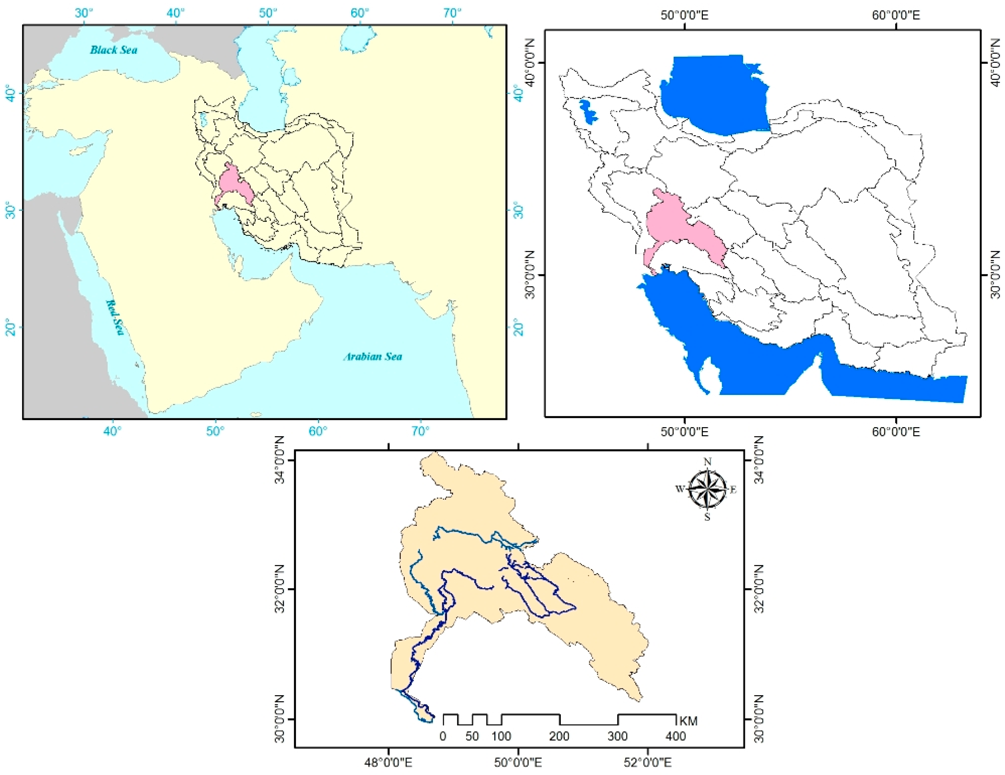
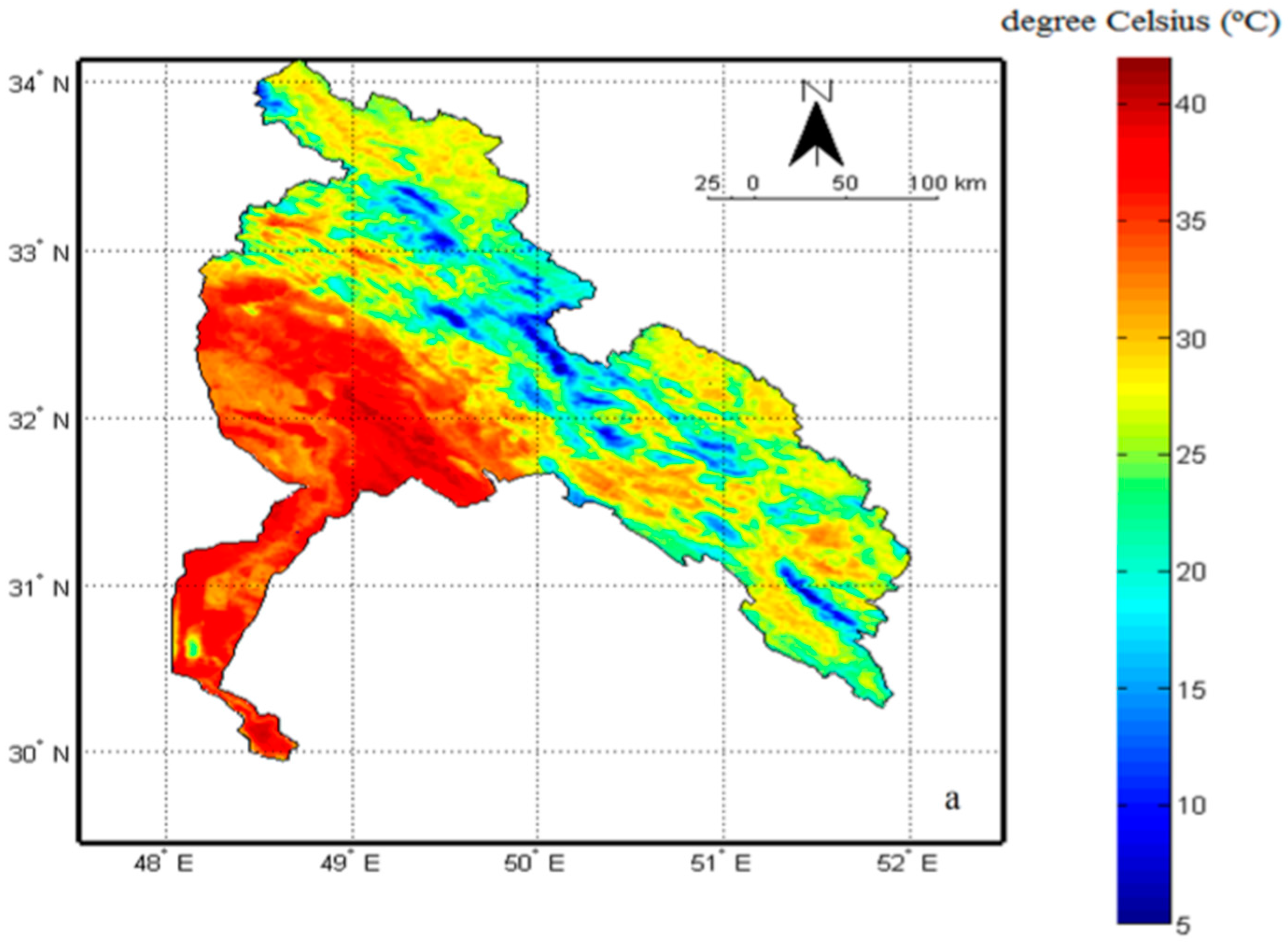
The Karoon River Basin is located in southwestern Iran with a total area of about 67,000 km2 and has a complex mountainous terrain. The largest rivers of Iran originate from the snow-covered areas of the Zagros Mountains that are located in this Basin, and the biggest dam reservoirs of the country are in this Basin as well. A location map of the study area is shown in Figure 1. The northern and eastern regions are characterized by mountains with elevations above 3000 m (Figure 2), while the south and southwestern regions are characterized by low elevations that rarely experience a seasonal snow cover because of a warm climate. The elevation ranges from 0 m at the Basin outlet to 4290 m at the highest point in the northern part of the Basin. The mean annual land surface temperature (LST) derived from MODIS Terra Land Surface Temperature (MOD11A1) (Figure 3a) is closely related to the elevation (Figure 2).
3. Data and Methods
3.1. Data
3.1.1. Snow Cover Products
In this study, the MODIS Terra (MOD10A1) and MODIS Aqua (MYD10A1) collection-5 products provided by the National Snow and Ice Data Center (NSIDC) were selected to examine seasonal spatial and temporal trends for SCD and SCA over the Karoon River Basin. The MODIS Terra (MOD10A1) and MODIS Aqua (MYD10A1) Snow Cover Daily L3 Global 500 m Grid contain data including snow cover, snow albedo, fractional snow cover, and quality assessment (QA) in the compressed Hierarchical Data Format-Earth Observing System (HDF-EOS) format. The spatial resolution of these products is 500 m and the projection is an equal area sinusoidal grid [15]. The time span of this study covered from 1 January 2003 to 31 December 2015. The h22v05 and h22v06 tile numbers covered the entire Basin and were selected for the analysis. In this study, more than 18,000 snow tiles were analyzed to illustrate snow cover changes over the Basin.
3.1.2. Station Data
In this investigation, daily snow depth data from nine synoptic stations operated by the Islamic Republic of Iran Meteorological Organization (IRIMO) were obtained from 1 January 2003 to 31 December 2012. The stations are mainly located in the lower elevations of the Basin (Figure 2). Snow depths of less than 1 cm were not included in the analysis. The snow depth data were used to evaluate the accuracy of the MODIS data in the study area.
3.1.3. Land Surface Temperature Data
We obtained MODIS Terra land surface temperature (LST) data (MOD11A1) that are freely available from (http://modis.gsfc.nasa.gov) for the time span from 1 January 2003 to 31 December 2015. The product is produced in tiles, with each tile containing 1200 rows by 1200 columns. The spatial resolution of the product is approximately 1 × 1 km on a daily time scale and is published in a sinusoidal projection [16]. The data are available from March 2000 to present. We used the tile numbers of h22v05 and h22v06 that entirely cover the study region. More than 9000 LST tiles were applied to analyze LST changes over the Basin. LST data were used to reveal the LST role on snow cover changes in the Basin.
3.1.4. Digital Elevation Model (DEM)
The Digital Elevation Model (DEM) for the tile numbers of h22v05 and h22v06 was downloaded from (ftp://landsc1.nascom.nasa.gov/outgoing/c6_dem/sin_500 m/). This DEM matched the snow data both in spatial resolution and projection system.
3.2. Methods
3.2.1. Cloud Gap-Filling Methods
The clear sky accuracy of MODIS in detecting snow reaches 93% [17]. The high accuracy of MODIS was documented by other studies throughout the world [18,19,20,21,22]. However, when clouds are present, the optical sensors cannot see through the clouds to identify the objects on the surface, so cloud cover is regarded as an important obstacle to surface snow detection. The application of methods aimed at minimizing the cloud cover effects is important for the use of daily snow cover data. In this study, we selected two common cloud removal methods to reduce cloud contamination [23,24]. In the first approach, MODIS Terra (MOD10A1) and MODIS Aqua (MYD10A1) were combined into a new data set. In this method, if a pixel value is coded snow (200) in either image, the pixel value of the resulting combined image is then coded snow. The theory of this method is based on the different pass times of Terra (morning) and Aqua (afternoon). Gao et al. [25,26] demonstrated that the combination of Terra and Aqua data could reduce the cloud cover effect by about 10%.
In the second approach, a temporal filtering was carried out for the combined data set. The temporal filtering was applied to determine the condition of cloud-covered pixels based on values from one day forward (t + 1) and one day backward (t − 1) with respect to a pixel on day t [26]. Thus, if the corresponding pixel of both the previous and following day were classified as snow, the cloudy pixel was also reclassified as snow [27]. This temporal combination method was also applied by [28,29]. Based on our newly developed data set (MOYD), we studied the seasonal trends in the SCD and SCA over the Karoon River Basin. We defined winter as the period from January to March, spring as the period from April to June, summer as the period from July to September, and fall as the period from October to December. After the preparation of the newly developed snow data set, we calculated the slope of the regression equations for all the pixels in the Basin, and the Mann–Kendall Rank Statistic was also applied to reveal temporal trends. As there is no snow cover in the Basin in summer, we only examined the trends for fall, winter, and spring.
The method is as follow:
The Mann–Kendall Rank Statistic, τ, was originally proposed by Mann (1945) and later improved by Kendall (1948), and determines if a trend exists in a series of xi values. To operationalize the calculations, all the xi values are replaced by their relative ranks, ki, ranging from 1 to N (lowest to highest values). The first term, k1, is compared with all later terms in the series from k2 to kN. A count is produced, n1, of the later terms whose values exceed k1. Next, a count is produced, n2, of the number of values from k3 to kN that exceed k2. This process continues, ending with the count for kN−1. A value of P is determined as:
and τ is then calculated as:
with the statistical significance of τ determined as:
where tg is the desired probability point of the Gaussian normal distribution appropriate to a two-tailed test. The value of the Mann–Kendall statistic approaches +1 for a strong upward trend and −1 for a strong downward trend (similar to the interpretation for a Pearson product-moment correlation coefficient).
In the case of simple regression, the dependent (climatological) variable, Y, is compared to the time variable, X, which represents the year of record. The slope, b, represents the change in Y with a change in X and is computed as:
which shows the annual linear change in Y. The significance of b is determined using a t-statistic, calculated simply as:
where sb is the standard error of b determined as:
where are the estimates of Yi based on the linear regression equation.
3.2.2. Trend Analysis
Before calculating the trend for the time series of SCD and SCA, the data were tested for normality (a Gaussian distribution) using the Kolmogorov–Smirnov one-sample test in which a variable is tested against another variable defined as having a normal distribution [30,31,32,33]. This test is similar to a t-test determining whether two variables were drawn from different populations. If the Kolmogorov–Smirnov test was statistically significant, we rejected the hypothesis that the observed data follow the normal distribution. Having tested the data for normality, we tested for trends using the simple regression analysis to determine if a significant linear trend existed in any of the seasonal variables. The climate values (SCD and SCA) were the dependent variables and the year of record served as the independent variable in the simple regression analyses. We also calculated the Mann–Kendall Trend Statistic for the various time series; this robust test does not assume a normal distribution in the variables being tested.
4. Results
4.1. Accuracy Assessment
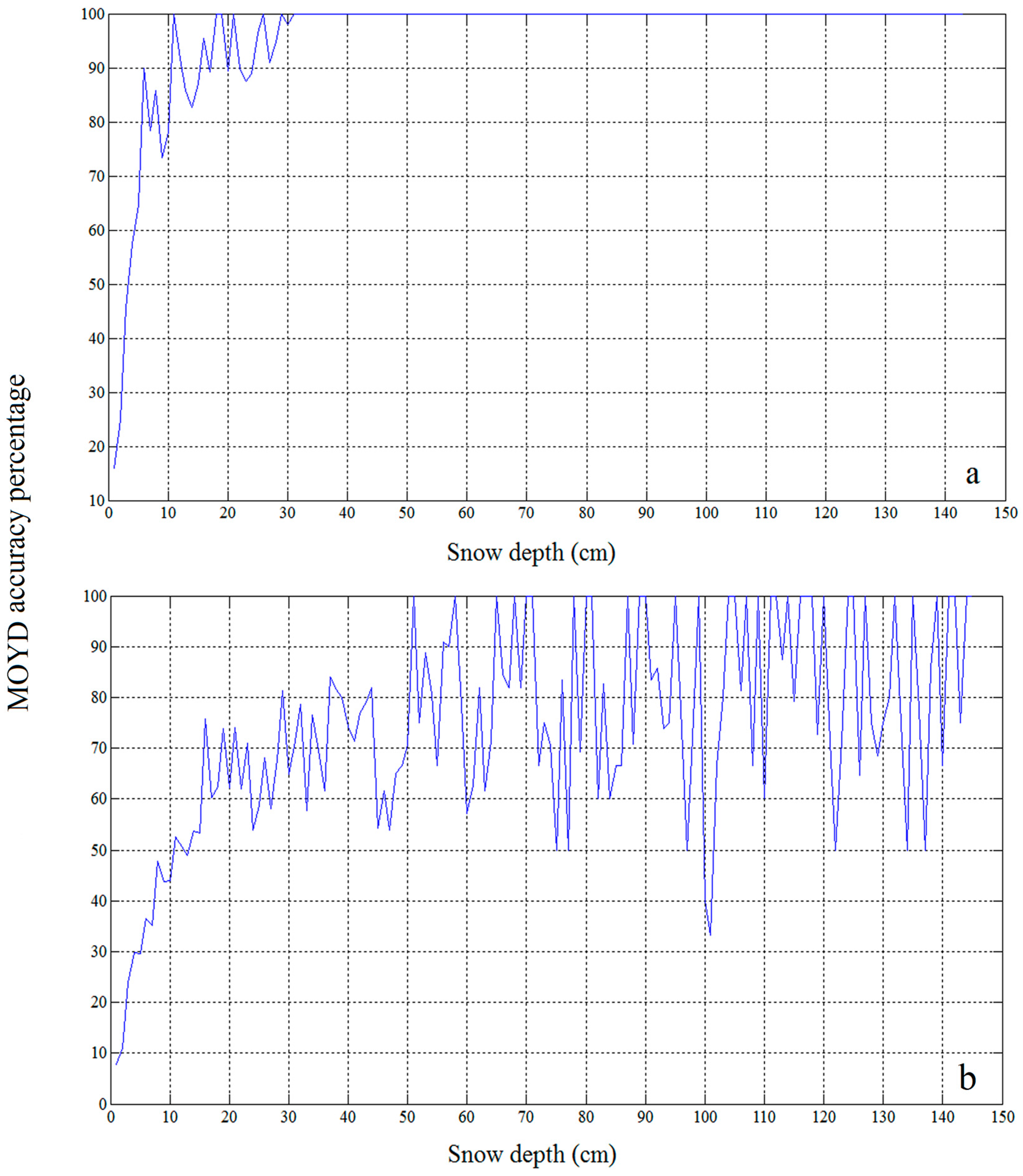
Snow depth observations at the selected stations were considered as ground truth for the pixel that was closest to each station. These pixels were regarded as snow-covered when the measured snow depth exceeded or was equal to 1 cm, and snow-free otherwise. Only snow depths ≥1 cm were included in the analysis. Also, only the cloud-free observations of the representative pixels were considered to evaluate MOYD accuracy under clear sky conditions (Figure 4a). If the MODIS pixel recorded snow and the station observation recorded snow as well, then for that time and that station we put “1”, but if the MODIS pixel recorded no snow and the station recorded snow, we put “0”. We then summed up all the “1” and divided the result by the number of observations. The few instances when no data could be produced in the cloud gap-filled MOYD dataset (<1%) were not included in the analysis. The results of the accuracy assessment of MOYD under clear sky for each snow depth classification are depicted in Figure 4a. It is important to note that the snow depths were not binned into categories in Figure 4. The accuracy percentage was above 80% for snow depth greater than 10 cm for clear sky conditions. The accuracy percentage increased to 100% for snow depths greater than 30 cm (Figure 4a). The detection of thin snow covers (e.g., <5 cm) is problematic even in clear sky conditions. Our findings are comparable to those from other studies: using the snow depth data of 20 climatic stations in Northern Xinjiang, China, Wang et al. [34] found that under clear sky conditions, the MODIS had high accuracy when mapping snow (94%) at snow depth ≥4 cm, but a very low accuracy (39%) for patchy snow or thin snow depths (<4 cm). Using 15 stations over the Upper Rio Grande Basin (Colorado and New Mexico), Klein and Bernett [18] showed that the majority of the days when MODIS failed to map snow occured when snow depth was less than 4 cm.
Snow depths were reported from the stations at 6:00 a.m. local time. However, the satellite pass time was several hours later. This time lag could allow a thin snow depth to be melted before the pass of the satellite. Therefore, part of the error in detecting thin snow cover may be attributable to this time difference.
The effectiveness of the MOYD data set in minimizing cloud cover effects was also calculated. The accuracy assessment described above was repeated without screening for cloud-free conditions in the MOYD. The results are depicted in Figure 4b. As can be seen from Figure 4b, the accuracy percentage decreased when cloudy sky conditions were taken into consideration. The accuracy percentage was ~50% for snow depths of 10 cm (Figure 4b). While the accuracy percentage generally increases with depth during cloudy conditions, reaching 100% for numerous depths, it was highly variable in our observations (Figure 4b). This was likely due to the lower frequency of deep snow covers at the observation sites. For example, ~1% of the observations displayed depths between 95 cm and 105 cm, and the accuracy percentage ranged from 35% to 100% over these depths (Figure 4b), owing to the great range in cloud cover during these infrequent observations. It is important to note that, by applying the cloud removal methods, up to 30 SCD were added to the annual mean compared to the raw data (MOD10A1) (Figure 5).
4.2. Karoon River Basin Snow Cover
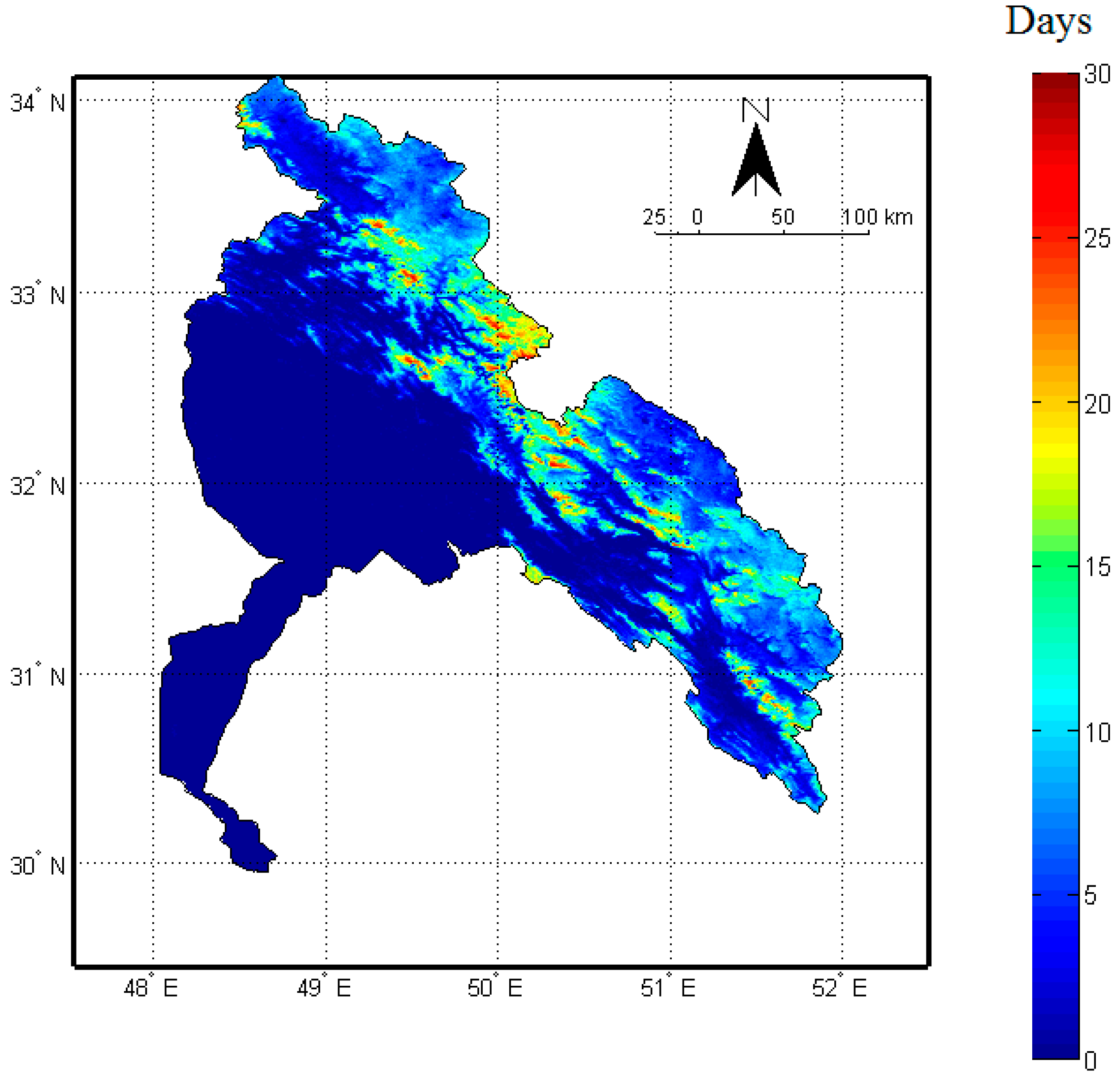
In the studied period, the annual average of SCD per year on the Karoon River Basin was less than 20 days for the majority of the area (Figure 3b). The average annual SCD exceeded 80 days over the higher elevation areas, with the highest elevations averaging more than 120 SCD (Figure 2 and Figure 3b). SCD is strongly related to elevation and temperature. A nearly perfect linear relationship (r2 = 0.92) exists between SCD and elevation, with a one-day increase occurring for every 15.4 m of elevation (Equation (1)). The relationship is even stronger (r2 = 0.98) when SCD is compared directly with the LST: SCD decreases by 5.5 days for every increase of 1 °C (Equation (2)). These results suggest that the elevation (and the highly-related mean temperature) controls SCD significantly. As the snowline responds to temperature, a warmer climate leads to a higher snowline, and the area available for the snow to accumulate decreases with increasing elevation. Therefore, the SCD–Elevation relation may be useful for understanding the shrinkage of the snow reservoirs.
SCD = −110.91 + 0.06472 Mean of Elevation
SCD = 168.59 − 5.4831 Mean of LST
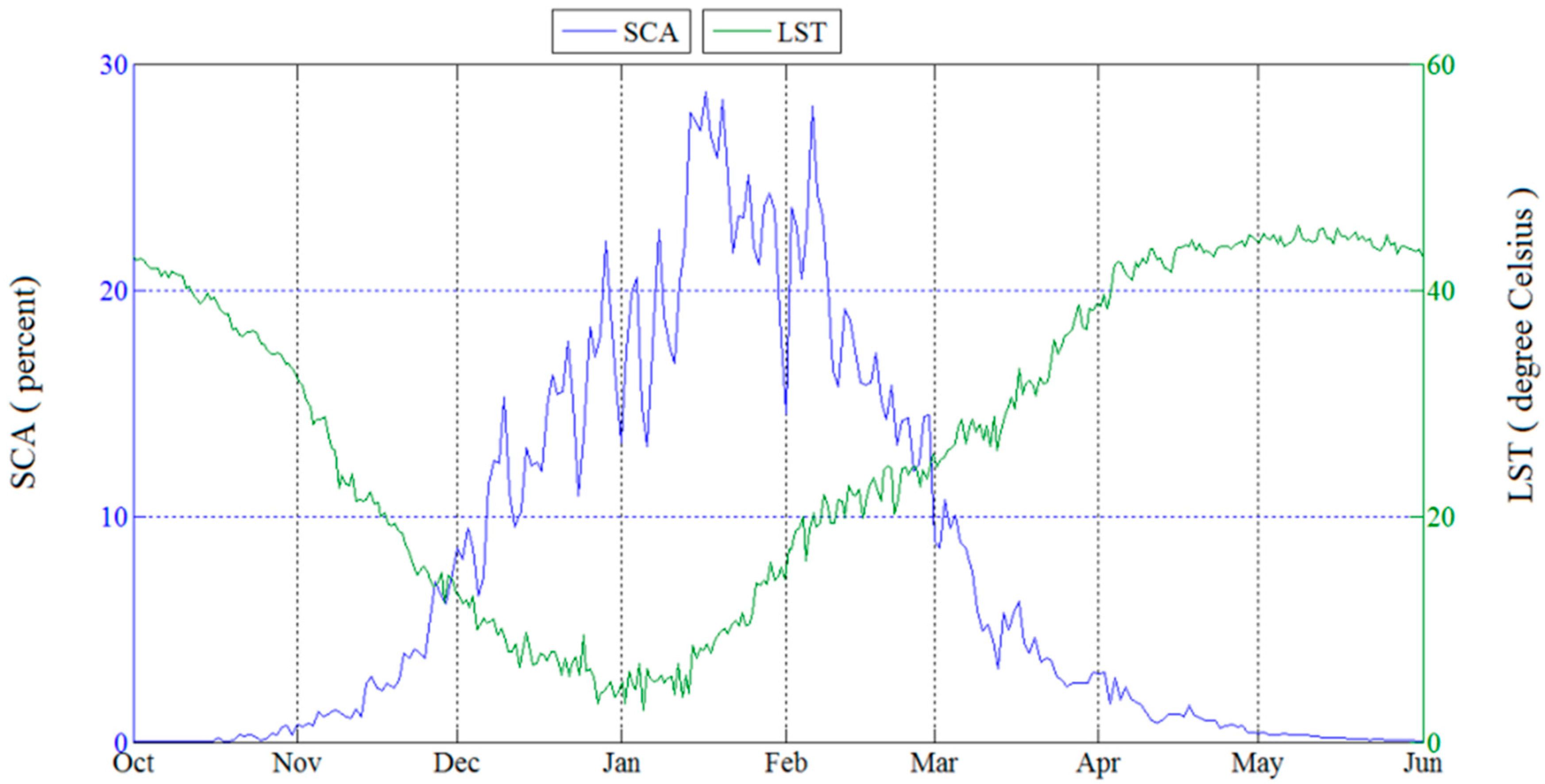
The seasonal evolution of the Basin SCA appeared to peak in mid-January, approximately two weeks after the minimum in LST occured in early January (Figure 6). From December to early February, the variability in SCA was large (Figure 6). For example, there was nearly 30% SCA in mid-January, decreasing to 15% by February, and then increasing to above 25% before mid-February. The majority of the Basin was warmer than the melting point in winter, suggesting that the SCA variability was caused by storm events depositing snowfall at low elevations, thus greatly increasing SCA, with the snowline rapidly retreating to higher elevations after the storm. In late February, the LST was the warmest (>12 °C) since early November and the SCA was less variable, declining steadily and rapidly (~10% per month) until late-March (Figure 6). The rate of SCA decrease slowed substantially after late-March, as snow cover persisted for more than 100 days at elevations above 3260 m, and for nearly 150 days at 4000 m elevation (Equation (2)). It is important to note that care needs to be taken when investigating the correlation between snow products, LST, and elevation because the MODIS collection 5 snow products also has a significant cutoff based on LST thresholds, e.g., if LST >283 K, the snow flag is set to no snow.
4.3. Trends in SCA and SCD
The seasonal SCA data showed no deviation from normality for the fall, winter, or spring seasons. The simple regression analysis revealed no significant trends in the seasonal data, and none of the Mann–Kendall trend statistics had an absolute value >0.393, which is needed for significance at the 0.05 level of confidence. While there were no significant trends in the SCA data, the regression analysis revealed that variations in SCA were strongly (p < 0.01) related to variations in LST.
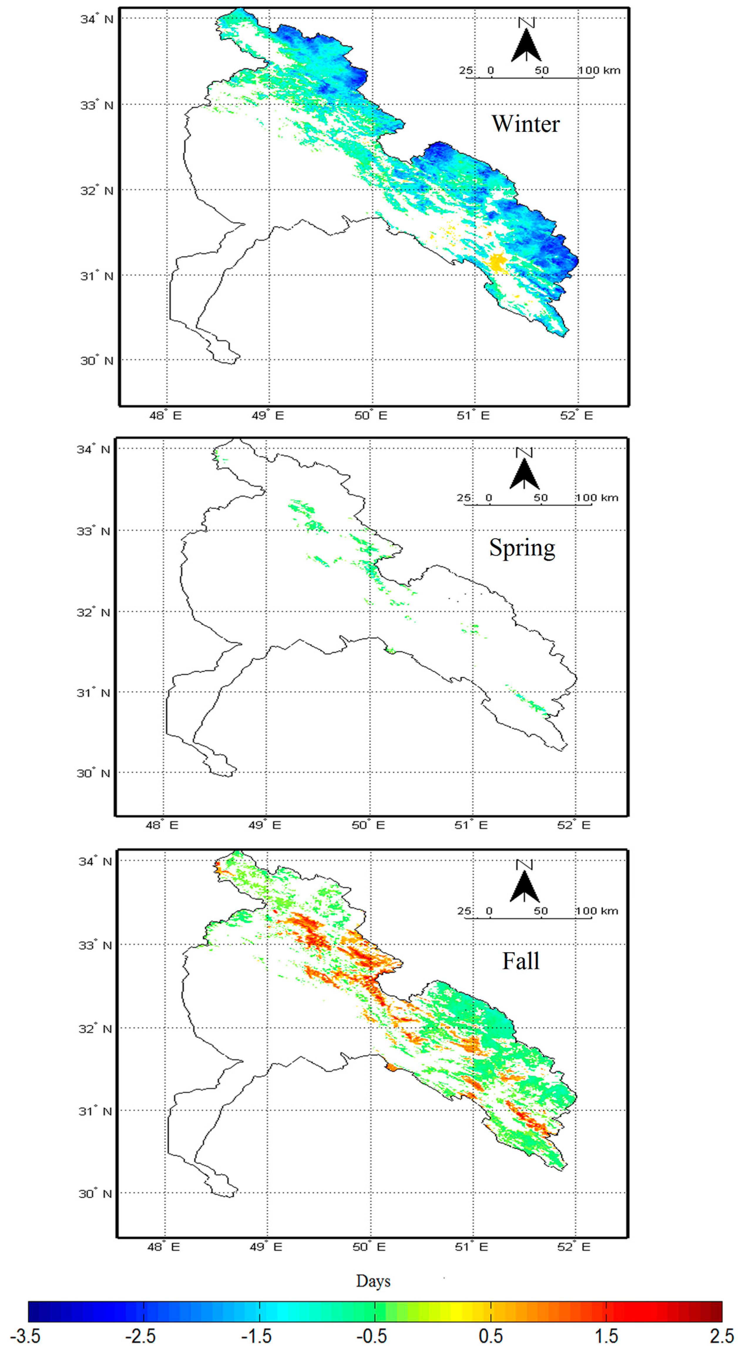
A significantly decreasing linear trend in winter SCD was evident (Figure 7), with the rate of the decrease reaching more than 2.5 days per year in some parts of the Basin, especially along the northeast border of the Basin. A significantly increasing trend of SCD could be seen in southern parts of the Basin, with a rate of nearly 1 day per year. In winter, nearly 43% of the Basin displayed a negative trend and only 1.4% experienced a positive trend for SCD (Table 1). The regression equation over the entire Basin with SCD as the dependent variable and Basin-wide LST as the independent variable was
Winter SCD = 42.82 − 2.536 Winter LST
The r2 value was 0.77 and the p value associated with the regression coefficient was <0.01. This highly significant result indicated a strong covariance between SCD and temperature across the Karoon Basin.
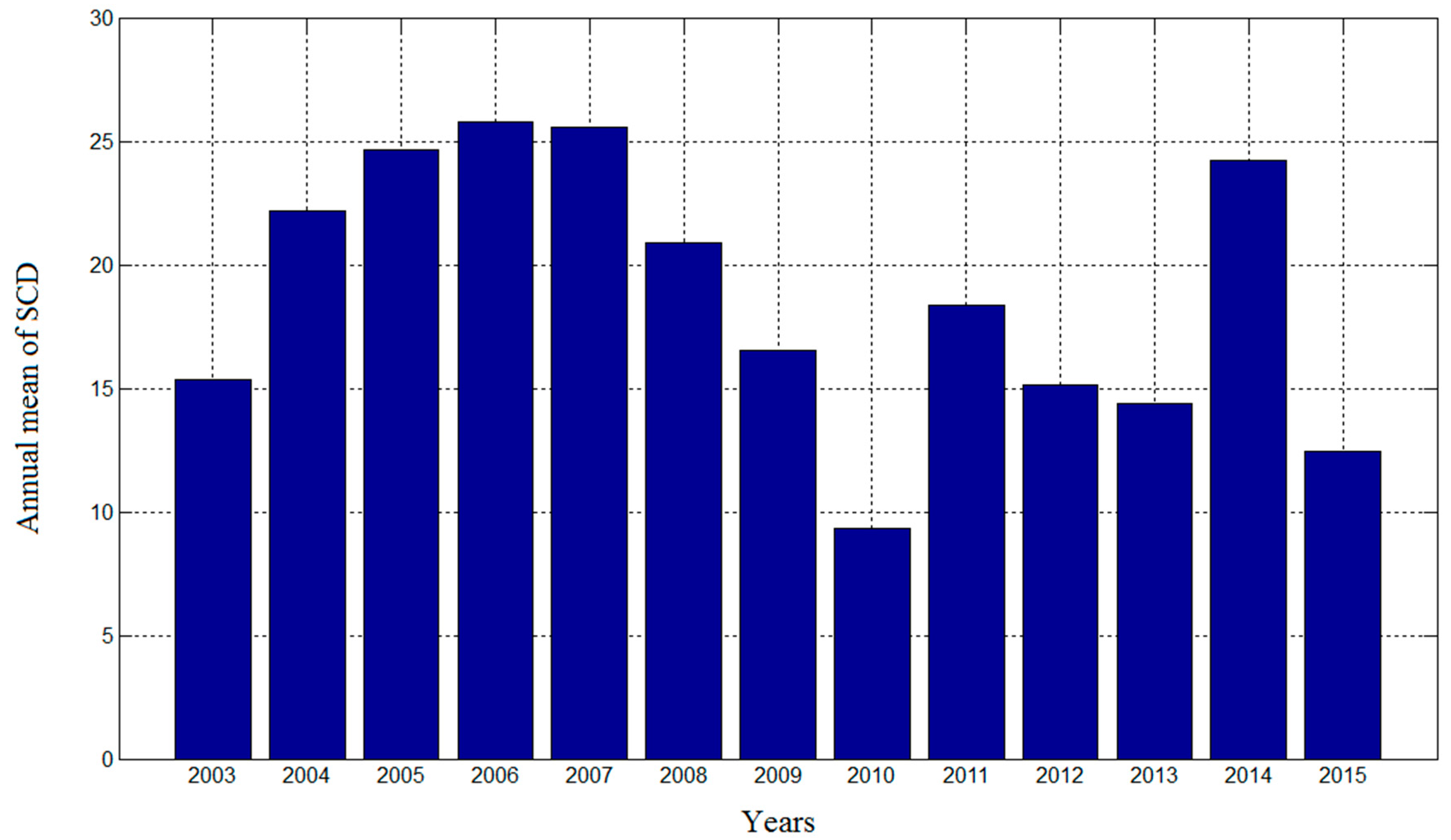
Trends in SCD in the fall and spring seasons were far less evident compared to winter. In fall, the areas with significant decreasing or increasing trends covered 25.35% and 10.38% of the Basin, respectively (Table 1). Similar to winter, the regression analysis showed a highly significant (p < 0.01) relationship with LST, with a loss of 1.21 SCD per 1 °C increase in temperature. In spring season, nearly 3.5% of the Basin had a significant negative trend but only 0.01% had a significantly increasing trend (Table 1). We produced an annual time series of SCD values from 2003 to 2015; the linear regression (and a Mann–Kendall test) indicated a slight downward trend that was not statistically significant. (Figure 8).
4.4. Trend in SCD in Elevation Classes
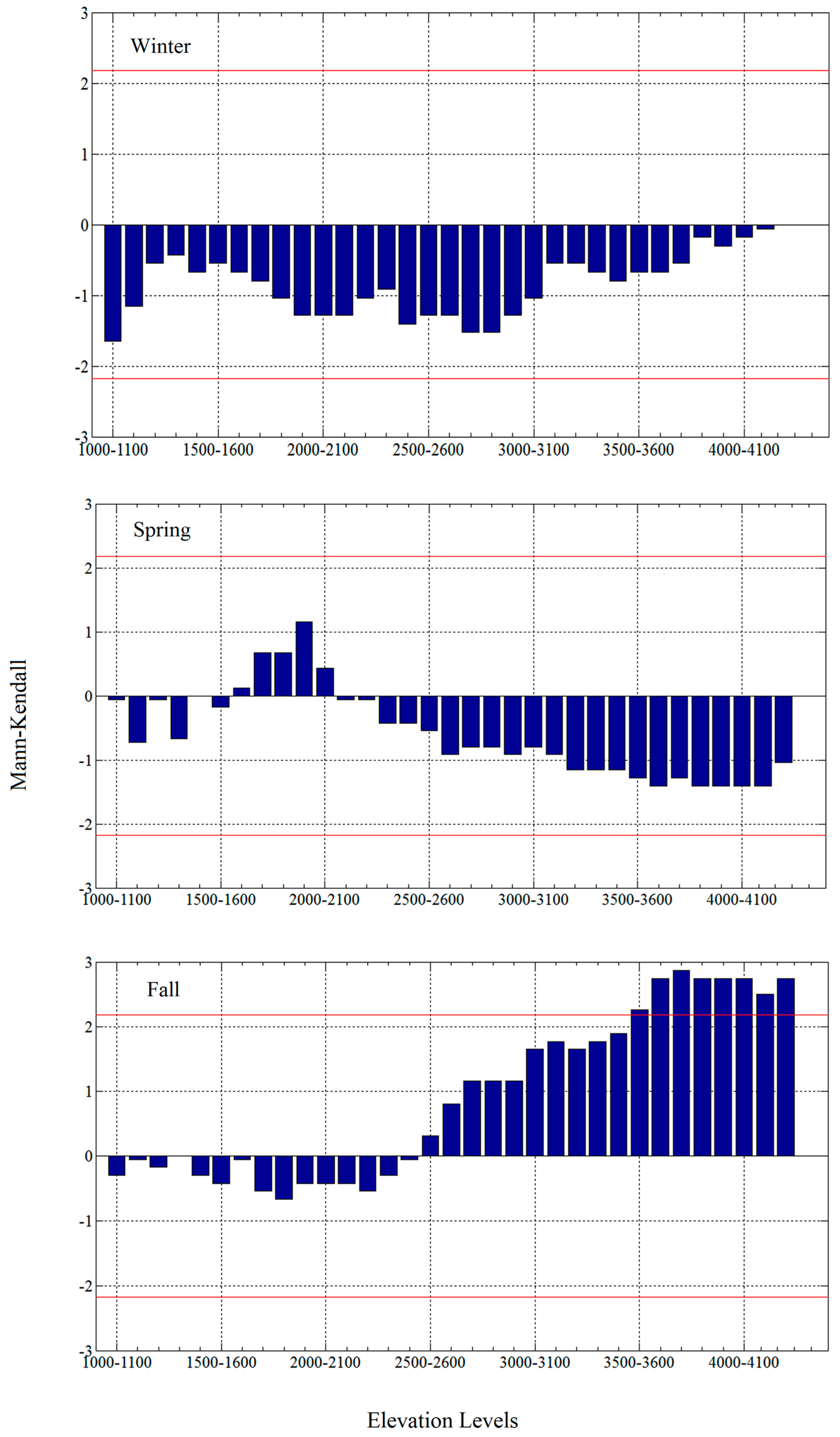
Figure 9 shows the Mann–Kendall scores for the elevation levels in winter, spring, and fall, respectively. We calculated the mean of SCD for each elevation interval of 100 m in each year from 2003 to 2015, and then we performed the Mann–Kendall trend test for the SCD in each of the intervals. Since at elevations below 1000 m no snow cover was seen, these elevations were excluded from the analysis. In winter, the values showed a decline at all elevation classes, but this decline was not statistically significant. The decreasing trends in winter approached zero when increasing in elevation from 2500 m to 4000 m (Figure 9). This was likely due to persistent subfreezing temperatures at the highest elevations in winter, limiting the variability of SCD in winter.
The values in spring were also negative for most levels, but, as in winter, the trends were not significant, given the relatively short period of record. Above 2500 m, the negative trends in spring increased in magnitude with the elevation (Figure 9). The average annual SCD increased from ~40 days at 2500 m to greater than 100 days for elevations above ~3250 m. This suggested an increased persistence of the snowpack in spring at high elevations, possibly reducing the noise in the spring SCD time series.
The fall values revealed little changes in snow-covered days below 2500 m, but an upward trend in the time series appeared above that level. The critical t-values in the fall season exceeded the 2.18 value needed to be judged significant at the 0.05 level of confidence for all elevation classes above 3500 m. This somewhat unexpected finding may be related to the variability of the total precipitation or its frequency in the fall, as there was a small trend in the LST (−0.02 °C year−1) during fall across the Basin.
5. Discussion
The primary findings from this study were: (1) trends toward less SCD in winter (although not statistically significant) were most evident at mid-elevations (2000–3000 m above sea level); (2) while there was little evidence for an SCD trend in winter at high elevations (>3000 m above sea level), trends of less SCD in spring were most evident at high elevations; (3) high elevations displayed increases in SCD during the fall. Over 2 °C of warming is projected to occur over this region by the end of the 21st century [35]. Given the negative relationship between temperature and SCD (Equations (2) and (3)), it is possible that the trends toward lower SCD will continue in the future. However, given the positive relationship between elevation and SCD (Equation (1)), future trends could be modulated by both the elevation and the precipitation trends. It is possible that the lack of winter trends at high elevations is due to temperatures that are consistently sub-freezing. However, given the trends toward more SCD in fall at high elevations (Figure 2, Figure 7 and Figure 9), when solar radiation and melt rates are generally low compared to spring, it is possible that trends in the precipitations contribute to the trends in SCD found in this study. A more detailed future investigation of how precipitation and temperature impact SCD is necessary to fully support these claims. Knowing the elevations and seasons that are most sensitive to temperature and those that are most sensitive to precipitation would help identify areas of the basin that are most sensitive to future changes in the climate.
Many studies were performed to reveal trends for snow cover using remote sensing data. For instance, Singh et al. [11] examined the trend of snow cover over the Indus, Ganga, and Brahmaputra river Basins over 2000–2011. The findings revealed that the Indus Basin had a unique increasing trend in snow cover, whereas the Ganga and Brahmaputra Basins had no significant trend over this period. In another investigation, Sönmez et al. [36] examined the trend of snow cover over Turkey from 2002 to 2012 using Interactive Multisensor Snow and Ice Mapping System (IMS) data and, at the significance level of 0.95, they detected a negative trend for spring and summer, a positive trend for autumn, and a combination of negative and no trend for winter. Using the MODIS snow data from 2000 to 2009, Khadka et al. [37] revealed that over the Tamakoshi Basin in the Hindu Kush Himalayan region there was a negative trend in winter and spring snow cover, while autumn snow cover showed a positive trend for this period, but the results were not found to be significant at the 95% confidence level. In the two previous investigations, an upward trend in fall snow cover was reported, which is consistent with our results.
Investigations at similar latitudes with longer records revealed trends in the annual maximum snow line [36] and in the elevation at which snowfall transitions to rainfall [37], and both variables impact SCD. In the Pir-Panjal range of the Himalayas (~32.33° N, 77.50° E), Verdhen et al. [38] suggested that the yearly maximum snow line altitude increased by 11 m per year from 1983 to 2009. In the Salt River Basin of central Arizona USA (~33.90° N, 110.50° W), Svoma [39] found increasing trends in the elevation at which snowfall transitions to rainfall (a parameter also known as the snow level) from 1934 to 2007. Also in the Salt River Basin, Ellis and Sauter [40] found a positive statistical relationship between the fraction of precipitation falling as snow and the ratio of runoff to precipitation, suggesting that a more efficient runoff on the Basin occurred with lower snow levels. The fraction of precipitation falling as snow was also found to influence the seasonal distribution of the runoff, suggesting that higher snow levels result in a higher portion of annual runoff occurring in winter [40]. Future research on the Karoon River Basin should focus on the effects of snow cover on runoff efficiency and timing. This information could be useful for water resource management if declining trends in SCD continue.
6. Conclusions
Daily time series of MOD10A1 and MYD10A1 from 2003 to 2015 were processed in order to reveal possible trends in snow covered days (SCD) and snow covered areas (SCA) in the Karoon River Basin. Land surface temperature data (MOD11A1) were also obtained to explore LST relation with SCD. Both positive and negative trends for SCD could be seen on seasonal scales. In winter, the area which had a significant negative trend covered 43% of the Basin, while only 1.4% of the Basin experienced a positive trend in SCD. In spring, nearly 3.5% of the Basin had a decreasing trend, while 0.01% area showed a positive trend. In fall, nearly 10.3% of the Basin's areas showed a positive tendency for SCD, while nearly 25% experienced a negative trend. The seasonal trend analysis of SCD for each of the elevation groups revealed decreasing trends at most of the elevation levels in winter and spring, although none were significant at the 0.05 level of confidence. In contrast, during fall, all elevation classes above 3500 m were judged to have a significant increasing trend at the 0.05 level of confidence. The results for seasonal SCA revealed that snow cover in winter, spring, and fall declined over the studied period, but in no case was the trend judged to be statistically significant at the 0.05 level of confidence.
The decreasing tendency of snow cover in the Basin could have many adverse effects for this region given that the largest rivers in the country flow in this Basin, and given that the projected winter warming over the region of 2–3 °C by 2100 [35] can exacerbate the conditions in the region even more. Further study on the Karoon River Basin should focus on the effects of precipitation and temperature on snow cover, which could identify areas of the Basin most sensitive to future warming.
Supplementary Materials
Supplementary File 1Acknowledgments
We are grateful to Ross Brown for all of the contributions to this paper. We certify that none of the authors of this paper has any conflict of interest.
Author Contributions
Mohammad Sadegh Keikhosravi Kiany and Seyed Ablofazl Masoodian analyzed the satellite data along with writing some parts of the paper. Robert C. Balling, Jr. and Bohumil M. Svoma contributed to the interpretation of the results and in the discussion. All authors contributed equally to the research.
Conflicts of Interest
The authors declare no conflict of interest.
References
- Brown, R.D. Northern hemisphere snow cover variability and change, 1915–97. J. Clim. 2000, 13, 2339–2355. [Google Scholar] [CrossRef]
- Leathers, D.J.; Mote, T.L.; Grendstein, A.J.; Robinson, D.A.; Felter, K.; Conrad, K.; Sedywitz, L. Associations between continental-scale snow cover anomalies and air mass frequencies across eastern North America. Int. J. Climatol. 2002, 22, 1473–1494. [Google Scholar] [CrossRef]
- Turner, J. Atlas of satellite observations related to global change. Weather 1994, 49, 226–227. [Google Scholar] [CrossRef]
- Tekeli, Y.; Tekeli, A.E. A technique for improving MODIS standard snow products for snow cover monitoring over Eastern Turkey. Arab. J. Geosci. 2012, 5, 353–363. [Google Scholar] [CrossRef]
- Elder, K.; Dozier, J.; Michaelsen, J. Snow accumulation and distribution in an alpine watershed. Water Resour. Res. 1991, 27, 1541–1552. [Google Scholar] [CrossRef]
- Anderton, S.P.; White, S.M.; Alvera, B. Evaluation of spatial variability in snow water equivalent for a high mountain catchment. Hydrol. Process. 2004, 18, 435–453. [Google Scholar] [CrossRef]
- Trujillo, E.; Ramfrez, J.A.; Elder, K.J. Topographic, meteorologic, and canopy controls on scaling characteristics of the spatial distribution of snow depth fields. Water Resour. Res. 2007, 43. [Google Scholar] [CrossRef]
- Zhou, X.; Xie, H.; Hendrickx, J.M.H. Statistical evaluation of remotely sensed snow-cover products with constraints from streamflow and SNOTEL measurements. Remote Sens. Environ. 2005, 94, 214–231. [Google Scholar] [CrossRef]
- Tang, Z.; Wang, J.; Li, H.; Yan, L. Spatiotemporal changes of snow cover over the Tibetan plateau based on cloud-removed moderate resolution imaging spectroradiometer fractional snow cover product from 2001 to 2011. J. Appl. Remote Sens. 2013, 7. [Google Scholar] [CrossRef]
- Maskey, S.; Uhlenbrook, S.; Ojha, S. An analysis of snow cover changes in the Himalayan region using MODIS snow products and in-situ temperature data. Clim. Chang. 2011, 108, 391–400. [Google Scholar] [CrossRef]
- Singh, S.K.; Rathore, B.P.; Bahuguna, I.M.; Ajai. Snow cover variability in the Himalayan—Tibetan region. Int. J. Climatol. 2011, 34, 446–452. [Google Scholar] [CrossRef]
- Wang, W.; Huang, X.; Deng, J.; Xie, H.; Liang, T. Spatio-temporal change of snow cover and its response to climate over the Tibetan Plateau based on and improved daily cloud-free snow cover product. Remote Sens. 2015, 7, 169–194. [Google Scholar] [CrossRef]
- Tahir, A.A.; Chevallier, P.; Arnaud, Y.; Ashraf, M.; Bhatti, M.T. Snow cover trend and hydrological characteristics of the Astore River Basin (Western Himalayas) and its comparison to the Hunza Basin (Karakoram region). Sci. Total Environ. 2015, 505, 748–761. [Google Scholar] [CrossRef] [PubMed]
- Jin, X.; Ke, C.Q.; Xu, Y.Y.; Li, X.C. Spatial and temporal variations of snow cover in the Loess Plateau, China. Int. J. Climatol. 2014, 35, 1721–1731. [Google Scholar] [CrossRef]
- Riggs, G.; Hall, D.; Salomonson, V. MODIS Snow Products User Guide to Collection 5, 2006, Retrieved 15 January 2013. Available online: http://www.nsidc.org/data/docs/daac/modis_v5/dorothy_snow_doc.pdf (accessed on 21 October 2016).
- Crosson, W.L.; Al-Hamdan, M.Z.; Hemmings, S.N.J.; Wade, G.M. A daily merged MODIS Aqua–Terra land surface temperature data set for the conterminous United States. Remote Sens. Environ. 2012, 119, 315–324. [Google Scholar] [CrossRef]
- Hall, D.K.; Riggs, G.A. Accuracy assessment of the MODIS snow products. Hydrol. Process. 2007, 21, 1534–1547. [Google Scholar] [CrossRef]
- Klein, A.G.; Barnett, A.C. Validation of daily MODIS snow cover maps of the Upper Rio Grande River Basin for the 2000–2001 snow year. Remote Sens. Environ. 2003, 86, 162–176. [Google Scholar] [CrossRef]
- Maurer, E.P.; Rhoads, J.D.; Dubayah, R.O.; Lettenmaier, D.P. Evaluation of the snow-covered area data product from MODIS. Hydrol. Process. 2003, 17, 59–71. [Google Scholar] [CrossRef]
- Simic, A.; Fernandes, R.; Brown, R.; Romanov, P.; Park, W. Validation of vegetation, MODIS, and GOESCSSM/I snow-cover products over Canada based on surface snow depth observations. Hydrol. Process. 2004, 18, 1089–1104. [Google Scholar] [CrossRef]
- Parajika, J.; Blosch, G. Validation of MODIS snow cover images over Austria. Hydrol. Earth Syst. Sci. 2006, 10, 679–689. [Google Scholar] [CrossRef]
- Huang, X.; Liang, T.; Zhang, X.; Guo, Z. Validation of MODIS snow cover products using Landsat and ground measurements during the 2001–2005 snow seasons over Northern Xinjiang, China. Int. J. Remote Sens. 2011, 32, 133–152. [Google Scholar] [CrossRef]
- Wang, X.; Xie, H.; Liang, T.; Huang, X. Comparison and validation of MODIS standard and new combination of Terra and Aqua snow cover products in Northern Xinjiang, China. Hydrol. Process. 2009, 23, 419–429. [Google Scholar] [CrossRef]
- Xie, H.; Wang, X.; Liang, T. Development and assessment of combined Terra and Aqua snow cover products in Colorado Plateau, USA and Northern Xinjiang, China. J. Appl. Remote Sens. 2009, 3. [Google Scholar] [CrossRef]
- Gao, Y.; Xie, H.; Lu, N.; Yao, T.; Liang, T. Toward advanced daily cloud-free snow cover and snow water equivalent products from Terra-Aqua MODIS and Aqua AMSR-E measurements. J. Hydrol. 2010, 385, 23–35. [Google Scholar] [CrossRef]
- Gao, Y.; Xie, H.; Yao, T.; Xue, C. Integrated assessment on multi-temporal and multi-sensor combinations for reducing cloud obscuration of MODIS snow cover products of the Pacific Northwest USA. Remote Sens. Environ. 2010, 114, 1662–1675. [Google Scholar] [CrossRef]
- Paudel, K.P.; Andersen, P. Monitoring snow cover variability in an agropastoral area in the Trans Himalayan Region of Nepal using MODIS data with improved cloud removal methodology. Remote Sens. Environ. 2011, 115, 1234–1246. [Google Scholar] [CrossRef]
- Hall, D.K.; Riggs, G.A.; Foster, J.L.; Kumar, S.V. Development and evaluation of a cloud-gap-filled MODIS daily snow-cover product. Remote Sens. Environ. 2010, 114, 496–503. [Google Scholar] [CrossRef]
- She, J.; Zhang, Y.; Li, X.; Feng, X. Spatial and Temporal Characteristics of Snow Cover in the Tizinafu Watershed of the Western Kunlun Mountains. Remote Sens. 2015, 7, 3426–3445. [Google Scholar] [CrossRef]
- Kolmogorov, A. Confidence limits for an unknown distribution function. Ann. Math. Stat. 1941, 12, 461–463. [Google Scholar] [CrossRef]
- Smirnov, N.V. Table for estimating the goodness of fit of empirical distributions. Ann. Math. Stat. 1948, 19, 279–281. [Google Scholar] [CrossRef]
- Massey, F.J. The Kolmogorov-Smirnov test for goodness of fit. J. Am. Stat. Assoc. 1951, 46, 68–78. [Google Scholar] [CrossRef]
- Birnbaum, Z.W. Numerical tabulation of the distribution of Kolmogorov’s statistic for finite sample values. J. Am. Stat. Assoc. 1952, 47, 425–441. [Google Scholar] [CrossRef]
- Wang, X.; Xie, H.; Liang, T. Evaluation of MODIS snow cover and cloud mask and its application in Northern Xinjiang, China. Remote Sens. Environ. 2008, 112, 1497–1513. [Google Scholar] [CrossRef]
- Intergovernmental Panel on Climate Change (IPCC). 2013: Annex I: Atlas of Global and Regional Climate Projections; van Oldenborgh, G.J., Collins, M., Arblaster, J., Christensen, J.H., Marotzke, J., Power, S.B., Rummukainen, M., Zhou, T., Eds.; Cambridge University Press: Cambridge, UK; New York, NY, USA, 2013. [Google Scholar]
- Sönmez, I.; Tekeli, A.E.; Erdi, E. Snow cover trend analysis using Interactive Multisensor Snow and Ice Mapping System data over Turkey. Int. J. Climatol. 2014, 34, 2349–2361. [Google Scholar] [CrossRef]
- Khadka, D.; Babel, M.S.; Shrestha, S.; Tripathi, N.K. Climate change impact on glacier and snow melt and runoff in Tamakoshi Basin in the Hindu Kush Himalayan (HKH) region. J. Hydrol. 2014, 511, 49–60. [Google Scholar] [CrossRef]
- Verdhen, A.; Chahar, B.R.; Ashwagosha, G.; Sharma, O.M.P. Modeling Snow Line Altitudes in the Himalayan Watershed. J. Hydrol. Eng. 2015, 21. [Google Scholar] [CrossRef]
- Svoma, B.M. Trends in snow level elevation in the mountains of central Arizona. Int. J. Climatol. 2011, 31, 87–94. [Google Scholar] [CrossRef]
- Ellis, A.W.; Sauter, K. The significance of snow to surface water supply: An empirical case study from the Southwestern United States. Phys. Geogr. 2017, 38, 211–230. [Google Scholar] [CrossRef]
Figure 1.
General location of the Karoon River Basin in Iran.

Figure 2.
Digital elevation model and distribution of the applied synoptic stations across the Basin.
Figure 2.
Digital elevation model and distribution of the applied synoptic stations across the Basin.

Figure 3.
Mean annual land surface temperature (LST) based on MOD11A1 (2003–2015) (a); Mean annual snow-covered days (SCD) (days) across the basin based on MOYD (2003–2015) (b).
Figure 3.
Mean annual land surface temperature (LST) based on MOD11A1 (2003–2015) (a); Mean annual snow-covered days (SCD) (days) across the basin based on MOYD (2003–2015) (b).


Figure 4.
Accuracy of MOYD snow cover with respect to snow depth classes under clear sky (a) and under clear and cloudy sky (b). The accuracy percentage is 100% for clear sky conditions when the snow depth is greater than 35 cm.
Figure 4.
Accuracy of MOYD snow cover with respect to snow depth classes under clear sky (a) and under clear and cloudy sky (b). The accuracy percentage is 100% for clear sky conditions when the snow depth is greater than 35 cm.

Figure 5.
Map of the snow covered days (MOYD vs. MOD10A1).

Figure 6.
Seasonal evolution of the mean daily SCA and LST over the period 2003–2015.

Figure 7.
Spatial distribution of trends in SCD (days per year). Only statistically significant trends are displayed, otherwise the area is considered to have no trend (see Table 1).
Figure 7.
Spatial distribution of trends in SCD (days per year). Only statistically significant trends are displayed, otherwise the area is considered to have no trend (see Table 1).

Figure 8.
Annual time series of mean SCD from 2003 to 2015 in the Basin.

Figure 9.
Trends in the mean of SCD for each elevation level.


Table 1.
Percentage of the Basin area with positive, negative, and nonexistent trends in SCD at the 0.05 level of confidence.
Table 1.
Percentage of the Basin area with positive, negative, and nonexistent trends in SCD at the 0.05 level of confidence.
| Decreasing Trend | No Trend | Increasing Trend | |
|---|---|---|---|
| Winter | 42.98 | 55.61 | 1.40 |
| Spring | 3.48 | 96.49 | 0.01 |
| Fall | 25.35 | 64.26 | 10.38 |
© 2017 by the authors. Licensee MDPI, Basel, Switzerland. This article is an open access article distributed under the terms and conditions of the Creative Commons Attribution (CC BY) license (http://creativecommons.org/licenses/by/4.0/).
Share and Cite
MDPI and ACS Style
Keikhosravi Kiany, M.S.; Masoodian, S.A.; Balling, R.C.; Svoma, B.M. Spatial and Temporal Variations of Snow Cover in the Karoon River Basin, Iran, 2003–2015. Water 2017, 9, 965. https://doi.org/10.3390/w9120965
AMA Style
Keikhosravi Kiany MS, Masoodian SA, Balling RC, Svoma BM. Spatial and Temporal Variations of Snow Cover in the Karoon River Basin, Iran, 2003–2015. Water. 2017; 9(12):965. https://doi.org/10.3390/w9120965
Chicago/Turabian StyleKeikhosravi Kiany, Mohammad Sadegh, Seyed Abolfazl Masoodian, Robert C. Balling, and Bohumil M. Svoma. 2017. "Spatial and Temporal Variations of Snow Cover in the Karoon River Basin, Iran, 2003–2015" Water 9, no. 12: 965. https://doi.org/10.3390/w9120965
Note that from the first issue of 2016, this journal uses article numbers instead of page numbers. See further details here.