Spatial Downscaling of Suomi NPP–VIIRS Image for Lake Mapping †


1
Shaanxi Key Laboratory of Earth Surface System and Environmental Carrying Capacity, Northwest University, Xi’an 710127, China
2
College of Urban and Environmental Sciences, Northwest University, Xi’an 710127, China
3
CSIRO Land and Water, Canberra ACT 2601, Australia
4
School of Remote Sensing and Information Engineering, Wuhan University, Wuhan 430079, China
5
Chongqing Key Laboratory of Karst Environment, School of Geographical Sciences, Southwest University, Chongqing 400715, China
6
Beijing Laboratory of Water Resource Security, Capital Normal University, Beijing 100048, China
*
Author to whom correspondence should be addressed.
†
This is an extended work of the following conference paper: Huang, C.; Chen, Y.; Zhang, S. Mapping Lakewater area at sub-pixel scale using Suomi NPP-VIIRS imagery. In Proceedings of the 1st International Electronic Conference on Water Sciences, 15–29 November 2016; Sciforum Electronic Conference Series, Volume 1, 2016, f001; doi:10.3390/ecws-1-f001.
Water 2017, 9(11), 834; https://doi.org/10.3390/w9110834
Submission received: 29 July 2017
/
Revised: 26 October 2017
/
Accepted: 27 October 2017
/
Published: 30 October 2017
(This article belongs to the Special Issue Selected Papers from the 1st International Electronic Conference on Water Science)
Abstract
:Capturing the dynamics of a lake-water area using remotely sensed images has always been an essential task. Most of the fine spatial resolution data are unsuitable for this purpose because of their low temporal resolution and limited scene coverage. A Visible Infrared Imaging Radiometer Suite on board the Suomi National Polar-orbiting Partnership (Suomi NPP–VIIRS) is a newly-available and appropriate sensor for monitoring large lakes due to its frequent revisits and wide swath (more than 3000 km). However, it provides visible and infrared images at relatively coarse spatial resolutions, which would sometimes hamper the accurate mapping of lake shorelines. This study, therefore, proposes a two-step downscaling method that combines spectral unmixing and subpixel mapping to produce a finer resolution lake map from NPP–VIIRS imagery, which is then applied to delineate the shorelines of five plateau lakes in Yunnan Province, as well as the shoreline dynamics of Poyang Lake at three separate times. A newly published global water dynamic dataset is employed in this study to improve the downscaling method. Results suggest that the proposed method can generate a finer resolution lake map that exhibits more details of the shoreline than hard classification. The downscaling results of the Suomi NPP–VIIRS generally achieve higher than 75% accuracy, while the downscaling results of a Landsat-simulated fraction map could have accuracy higher than 85%. This reveals that errors and uncertainties exist in both procedures, but mainly come from the spectral unmixing procedure which retrieves water fractions from NPP–VIIRS data.
1. Introduction
Lakes are an important component of the regional water cycle. They play a significant role in the regional water balance of ecosystems. Lake water can sometimes change drastically because of climate change, irregular precipitation and varying consumption in arid and semi-arid regions [1,2]. Therefore, intensive mapping is necessary to capture the dynamics of lake-water areas for the purpose of water resource balance analysis [3,4].
Satellite imagery is an essential data source for lake-area monitoring because of its wide coverage and repeated observations [5]. Various remotely sensed images have been employed to serve this purpose, including synthetic aperture radar (SAR) images and optical images. SAR images, including Envisat [6] and Sentinel-1 [7,8], have been proven to be effective in mapping surface water dynamics or monitoring lake areas because they are not restricted to weather conditions or sunlight. Optical images, such as those of the Landsat Thematic Mapper (TM)/Enhanced Thematic Mapper plus (ETM+)/Operational Land Imager (OLI) [9,10,11], Advanced Very High Resolution Radiometer (AVHRR) [12,13], and Moderate Resolution Imaging Spectroradiometer (MODIS) [14,15,16], have also been widely used for lake-area monitoring because of their high data availability and suitable resolutions. Most of these prior studies have proved that the near-infrared (NIR) and short-wave infrared (SWIR) channels are most suitable for delineating water from land. In particular, the spectral characteristics of water in the SWIR channel are much more stable than those in the NIR channel [17,18].
The Suomi National Polar-orbiting Partnership (Suomi NPP) is a new generation of satellites intended to replace the Earth Observation System satellites [19]. The Visible Infrared Imaging Radiometer Suite on board Suomi NPP (Suomi NPP–VIIRS) provides a range of visible and infrared bands at a moderate resolution for observing the Earth’s surface. It is considered to be an upgrade and replacement of the AVHRR and MODIS as a wide-swath and multispectral sensor [20]. Its ability to detect surface water and lake-water areas has been tested in an exploratory study [21].
Landsat imagery is one of the most popular remote sensing data sources that have been used for mapping lakes or other types of surface water bodies because of its fine spatial resolution, mostly at regional or continental scale [22,23]. With the assistance of Google Earth Engine (http://earthengine.google.com), a new cloud platform for large satellite data analysis, several studies have mapped surface water dynamics at a global scale using Landsat data archives [24,25]. The results of Pekel et al. [24], in particular, have been recommended as providing the best understanding of global surface water dynamics so far [26]. However, restricted by the low temporal frequency of Landsat coverage, their results only provide monthly occurrences of water inundation. Therefore, their dataset might have missed some rapid surface water dynamics, especially those caused by flood events.
On the contrary, like other coarse resolution sensors, the Suomi NPP–VIIRS scans the Earth’s surface frequently with a broad view. It acquires images that provide a timely, cost-effective, and spatially comprehensive view of lake coverage. Unfortunately, these images have medium to coarse spatial resolutions, which hinders the accurate mapping and monitoring of lake-water areas. A traditional and widely used approach to overcome this limitation is the spatial downscaling method [12,18] that consists of the spectral unmixing method, which estimates the percentage of water (water fraction) in each mixed pixel, and the subpixel mapping (SPM) method, which allocates the water subpixels within the mixed coarse pixel.
Spectral unmixing is a procedure by which the measured spectrum of a mixed pixel is decomposed into a collection of endmembers, and a set of corresponding fractions that indicate the proportion of each endmember presented in the mixed pixel [27]. Owing to its definite physical meaning and simple calculation, the unmixing method based on the linear spectral mixture model (LSMM) is one of the most popular approaches [28]. It has been implemented in many studies for extracting surface water or lake-water areas [12,18,21,29]. There is a consensus that the major difficulty of LSMM is endmember selection [12,18,21], including the selection of water endmembers and non-water endmembers.
Subpixel mapping, or super-resolution mapping, is a technique generally used to retrieve a finer resolution land cover map from fraction images [30]. Many algorithms have been developed to spatially allocate subpixels within each coarse pixel of fraction maps, such as the Hopfield Neural Network [31], genetic algorithm [32,33], pixel-attraction models [34,35,36], pixel-swapping algorithms [37,38,39,40], and particle swarm algorithms [41]. Although these algorithms use different approaches, they are all based on the spatial correlation of land cover information, referring to the tendency of a land cover feature to be more alike than more distant observations. Therefore, it is obvious that this kind of method is applicable for mapping lake shorelines at subpixel scale. Several studies have implemented different subpixel mapping methods to derive finer-resolution shorelines or lake areas [42,43,44,45,46,47].
Although there are many studies, as mentioned above, that have either tried to retrieve water fractions using spectral unmixing, or allocate subpixel location using subpixel mapping, few of them integrate both together. This is because both procedures introduce uncertainties and errors once combined, and it would be difficult to evaluate and optimize each of them individually. This study, therefore, aims to present a complete spatial downscaling procedure from spectral unmixing to subpixel mapping, in order to produce finer resolution lake maps from Suomi NPP–VIIRS data. The global water dynamic dataset published by Pekel et al. [24] was employed to assist endmember selection and also subpixel allocation processes. The uncertainties introduced by each step of the procedure were carefully tested and examined. By doing this, this study aims to reveal whether the spatial downscaling method is able to describe lake shorelines at a higher spatial resolution and accuracy, and how reliable the downscaling results are. This paper is organized as follows. Study areas and materials involved are presented in Section 2. The section also gives a detailed description of the proposed downscaling method and the method for accuracy assessment. Section 3 shows the downscaling results and discusses their accuracy against Landsat data. The conclusions are presented in Section 4.
2. Materials and Methods
2.1. Study Areas and Materials
2.1.1. Study Areas
In order to demonstrate the applicability and generality of the proposed method in lake downscale mapping, two groups of case studies were selected. The first one is a large area that covers five lakes. While the water boundaries of these lakes are relatively stable, this case study intended to reveal the generality of the downscaling method in different lakes. The second group is a single lake with obvious water dynamics, intended to demonstrate the applicability of the downscaling method for monitoring lake-water variation at subpixel scale.
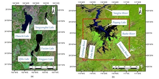
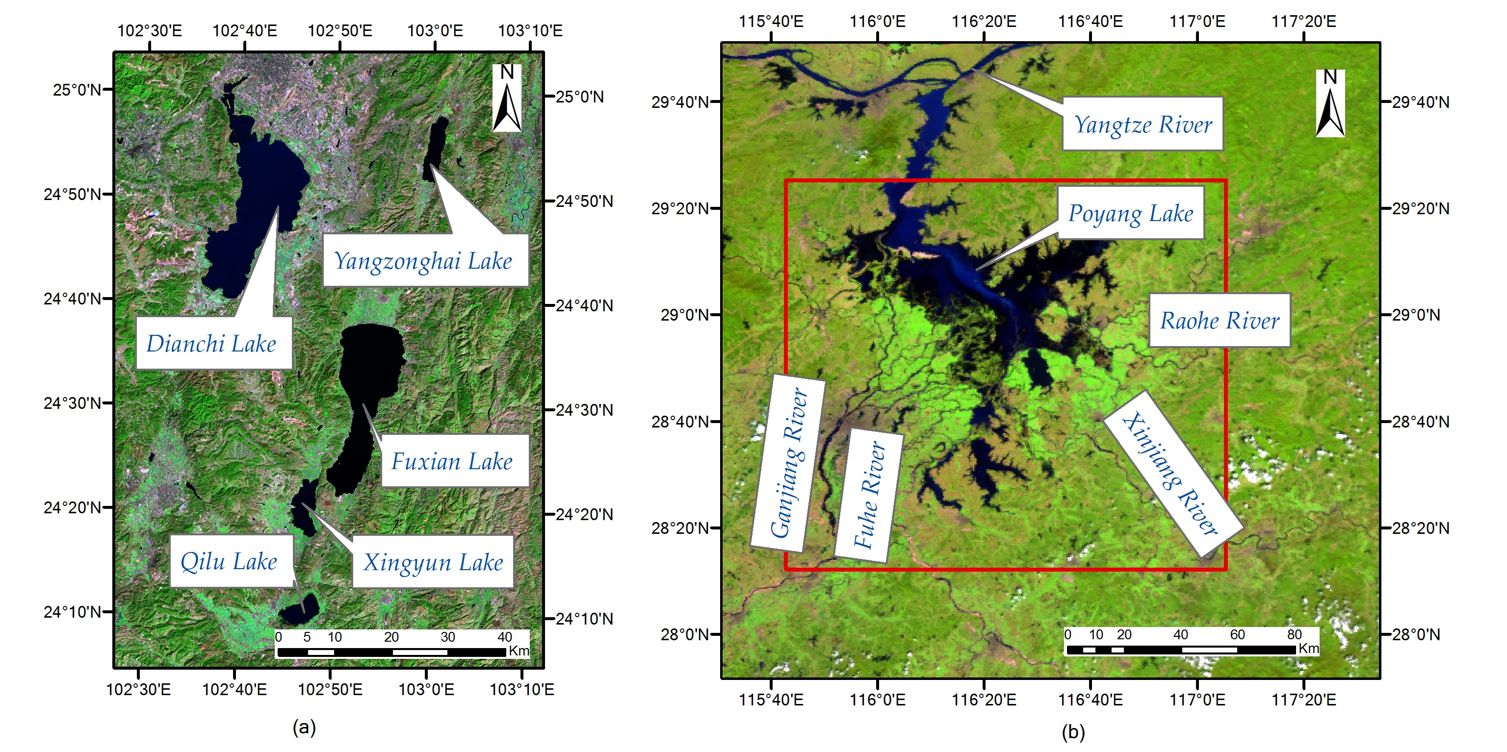
For the first group, an area that covers five of the largest plateau lakes in Yunnan Province of China, including Dianchi Lake, Fuxian Lake, Yangzonghai Lake, Xingyun Lake and Qilu Lake, was selected. It is located between 24°0′–25°1′ N and 102°5′–103°1′ E (Figure 1a). All these lakes are essential water resources for Yunnan Province. On one hand, they provide physical conditions for human life and socio-economic development. On the other hand, each of them is a key element of its local ecosystem and a major driver of changes in the ecosystem. The shapes of these lakes are quite different from each other. Dianchi Lake is the largest and its shape is also more intricate than the others, with a sand levee on the north splitting the lake into two parts. The smaller part on the north side is called the inner lake, with an area of approximately 10 km2. The other part is the outer lake with an area of almost 300 km2. The shorelines of the other four lakes are relatively simpler, except that there is a big wetland on the south-west of Qilu Lake which makes the mapping of its shoreline difficult. Furthermore, there are some tiny tributaries on the west of Xingyun Lake and south-west of Qilu Lake, which would also be difficult to map on coarse resolution images.
For the second group, Poyang Lake located on the south bank of the middle and lower reaches of the Yangtze River (Figure 1b), was selected as the study area. As the largest freshwater lake in China, Poyang Lake has a drainage area of more than 160,000 km2. With an overall decreasing trend, the water area of this lake fluctuates drastically between the wet and dry seasons. During the wet season, the floodplains are inundated, forming a big lake with a more than 3000 km2 water area. In the dry season, the water area can shrink to less than 1000 km2, leaving a narrow meandering channel [48]. For the sake of flood control and other management purposes, levees have been built around the lake, which creates numerous small lakes [49]. During the dry season in particular, the lake is usually divided into many connected and disconnected patches. Therefore, it is always difficult to define the exact boundary of Poyang Lake, because it changes obviously over time.
2.1.2. Materials
Two sets of image data, namely Suomi NPP–VIIRS and Landsat OLI, were used in this study. For the Yunnan lakes, only one pair of images acquired on 2 February 2014 were selected, while for Poyang Lake, three pairs of NPP–VIIRS and Landsat images, acquired either in the wet season or the dry season, were selected, considering data availability and cloud cover issues. There were drastic water-area changes between these three dates (T1, T2 and T3). The selected images are listed in Table 1.
Suomi NPP–VIIRS images were downloaded from the National Oceanic and Atmospheric Administration (NOAA)/Comprehensive Large Array-data Stewardship System (CLASS) (http://www.class.ncdc.noaa.gov/saa/products/search?datatype_family=VIIRS). Suomi NPP-VIIRS sensors provide 22 visible and infrared bands with wavelength ranging from 0.4 to 12.5 μm. Sixteen of them are moderate resolution bands (M-bands) at a resolution of 750 m. There is also a day/night band with 750 m resolution and five imagery resolution bands (I-bands) with 375 m resolution. The third I-band (I3), an SWIR band with a spectral range from 1.58 to 1.64 μm, was employed in this study to estimate water fraction because of the high separability of land and water in this part of the spectrum [17,18].
Landsat OLI images at 30 m resolution acquired on the same day as Suomi NPP–VIIRS images were downloaded from United States Geological Survey (USGS) EarthExplorer platform (https://earthexplorer.usgs.gov/). They were the standard terrain correction (Level 1T) product that has been radiometrically and geometrically corrected. They were used as the reference data to evaluate the accuracy of the downscaling results of the Suomi NPP–VIIRS because of their relatively finer spatial resolution. The time lag between the acquisition of NPP–VIIRS and Landsat is about 3 h. Band 6 of Landsat OLI has a wavelength range from 1.56 to 1.66 μm, which is close to that of the NPP–VIIRS I3 band. Both types of images have been atmospherically corrected and processed to surface reflectance in ENVI 5.1, and then co-registered with each other.
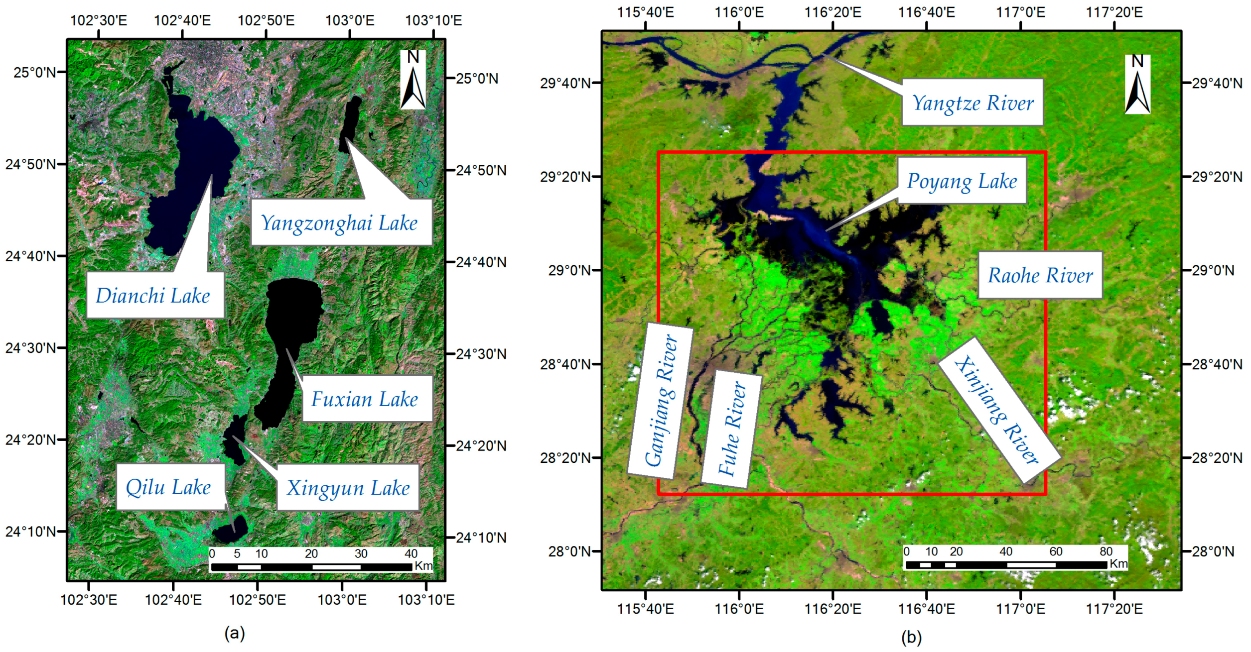
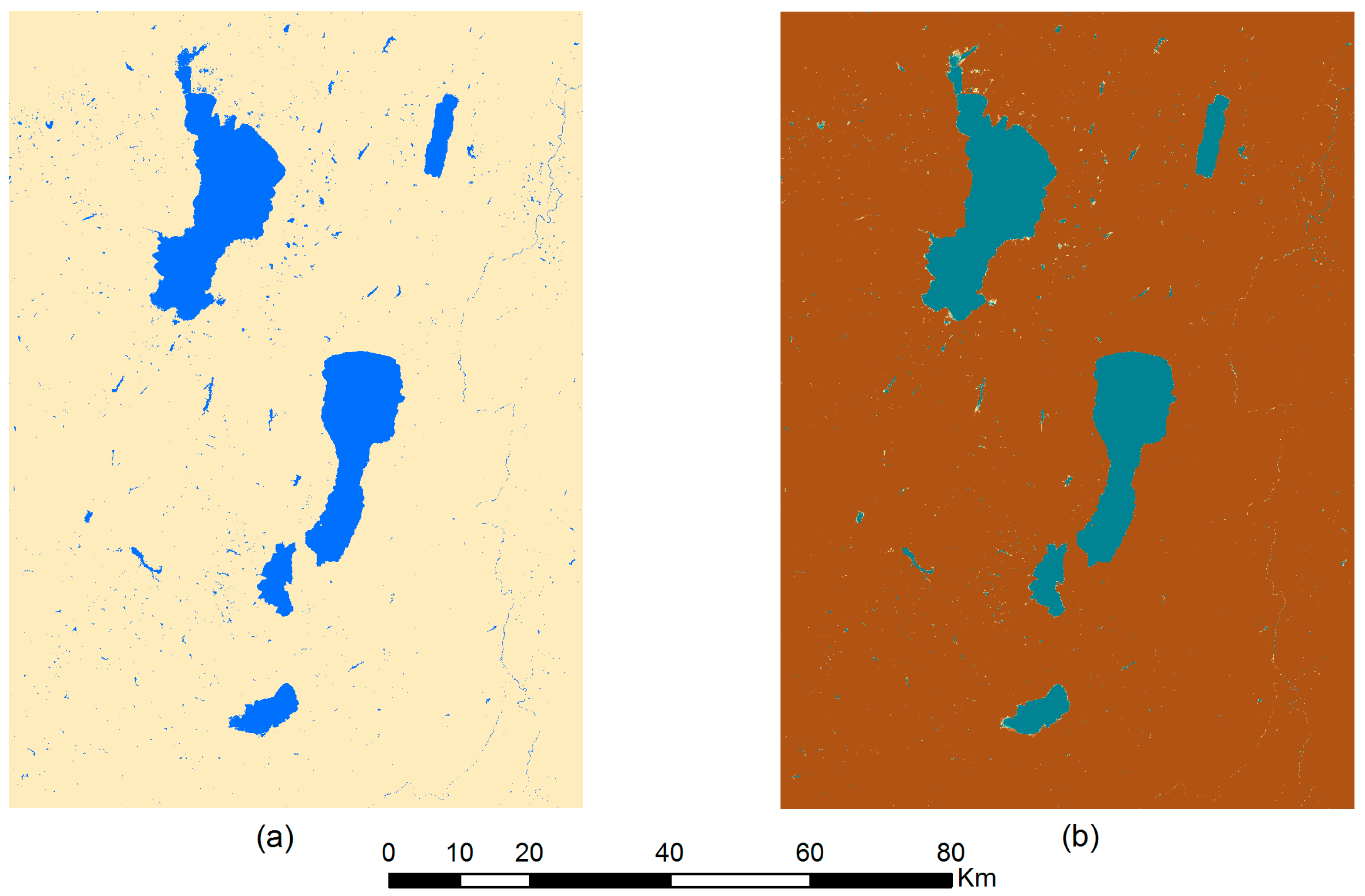
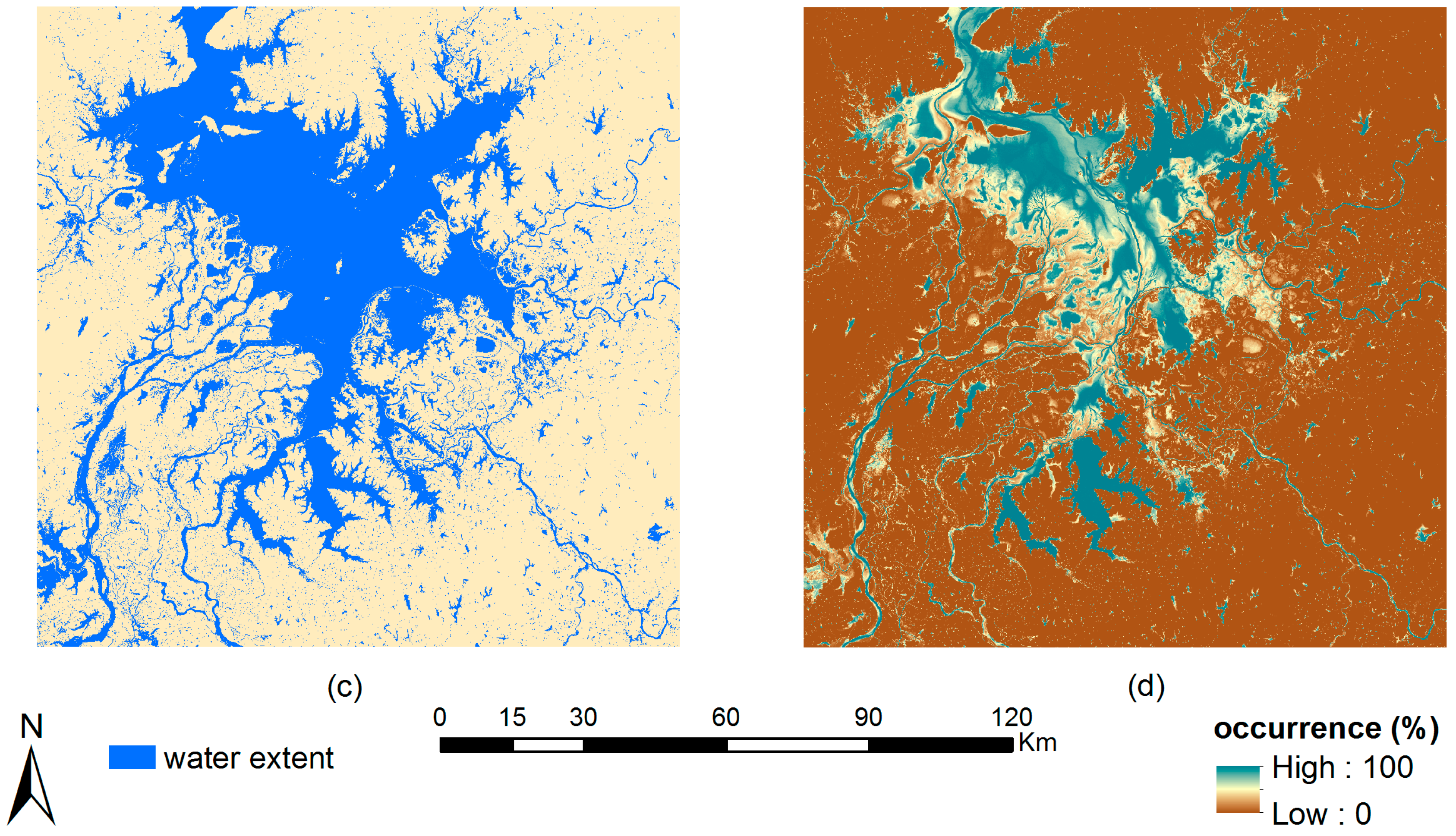
A 30 m resolution global surface water dynamic dataset (https://global-surface-water.appspot.com/), which was derived by Pekel et al. [24] using more than 3 million Landsat images over the past 32 years, was employed in this study as auxiliary data. This dataset includes a series of raster layers such as occurrence, change, seasonality, recurrence, transitions, and extent. Here, only extent and occurrence layers were used. The extent layer (e.g., Figure 2a,c) records the maximum water extent over the last 32 years. The occurrence layer (e.g., Figure 2b,d) maintains the frequency of water occurrence over the whole observation period in monthly time-steps. Permanent water bodies would in theory have an occurrence value of 100%, but this value is sometimes affected by cloud cover, which means some of the permanent water bodies have less than 100% occurrence. Through careful visual inspection, pixels with occurrence values greater than 90% were considered as permanent water bodies in these lake areas.
2.2. Methods
2.2.1. Water Fraction Retrieval
Water fraction retrieval was conducted on the basis of LSMM theory [50] which assumes the reflectance of a mixed pixel to be a linear combination of all its endmembers’ reflectance. According to LSMM, water fraction f can be estimated using the following equation:
where Rmix is the reflectance of a mixed pixel containing both water and land fractions; and Rwater and Rland are the reflectance of pure water and land, respectively.
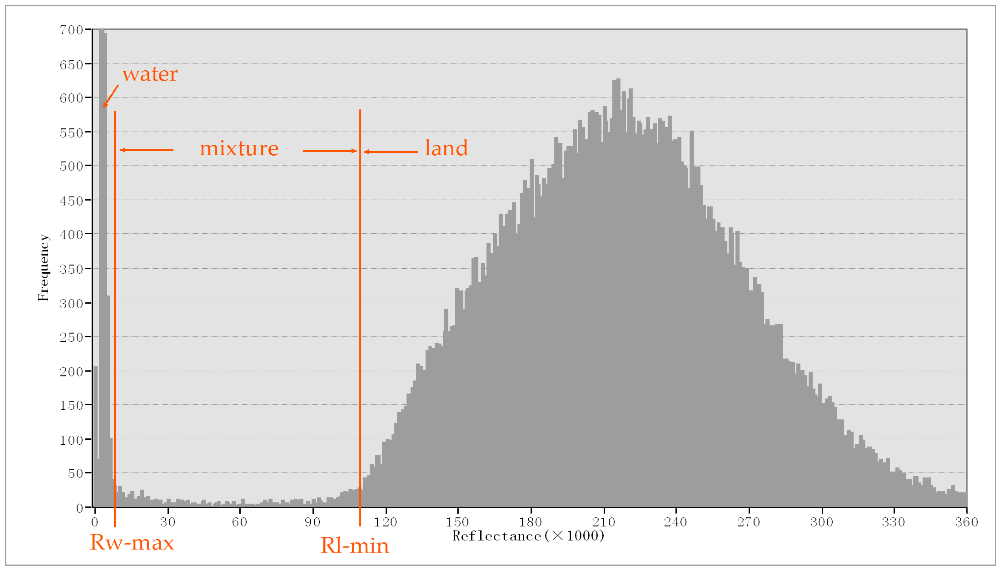
The value of Rmix can be identified directly from the reflectance image. Therefore, the most difficult part of using Equation (1) to estimate water fraction is to find optimal candidate pure pixels that can be used as Rwater and Rland. Huang et al. [21] determined feasible value ranges for Rwater and Rland from the histogram of the SWIR band (I3) of the NPP–VIIRS, considering this histogram generally appears as two peaks when there are enough water and land pixels on the image (an example is shown as Figure 3). The feasible range for pure water pixels starts from the minimum reflectance value of the whole image and ends with the maximum reflectance of a pure water pixel, while the feasible range for pure land pixels starts from the minimum reflectance of a pure land pixel and ends with the maximum reflectance value of the whole image. Therefore, the determination of feasible ranges is actually determining the upper limit of the pure water pixel range (Rw-max in Figure 3) and the lower limit of the pure land pixel range (Rl-min in Figure 3). A moving window was then applied to search for candidate pure pixels that have reflectance values within the feasible ranges. While the moving window approach reduced the uncertainties of reflectance variations of water and land objects to some extent, the determination of feasible ranges from the histogram still needs manual intervention, which introduces additional uncertainties [21].
In this study, the extent layer (e.g., Figure 2a,c) was employed to generate the maximum water mask to exclude possible water areas and extract pure land pixels. It was first resampled to a 15 m binary water map and then aggregated to 375 m resolution. The aggregated pixel would be considered as a pure land pixel if all the 15 m pixels in the aggregation window are non-water. The minimum reflectance of all these pure land pixels was selected as the lower limit for the feasible value range of pure land pixels (Rl-min in Figure 3). The occurrence layer (e.g., Figure 2b,d) was used to generate the permanent water mask at 375 m resolution, also through resampling and then aggregating. The aggregated pixel would be considered as a permanent water pixel only if all the 15 m pixels in the aggregation window are water. The maximum reflectance of all permanent water pixels was used as the upper limit for the feasible value range of pure water pixels (Rw-max in Figure 3). It has to be noted that when selecting the minimum reflectance of all pure land pixels and the maximum reflectance of all pure water pixels, the three-sigma rule was applied in order to avoid abnormal values being wrongly selected. The three-sigma rule considers values that lie out of three standard deviations of the mean to be outliers, which are usually taken as abnormal values.
Once the feasible ranges for both pure water and pure land pixels were determined, mixed pixels could be identified easily. A 3 × 3 moving window was applied to determine the endmembers for each mixed pixel. Among all the pure land pixels within the moving window, the one that has the lowest reflectance value was taken as the endmember of land (Rland). The endmember of water (Rwater) was determined similarly by taking the highest reflectance value of all the pure water pixels within the moving window. These two endmembers were then employed to estimate the water fraction of each mixed pixel using Equation (1).
2.2.2. Subpixel Mapping
After the derivation of the water fraction, subpixel mapping is needed to allocate subpixels within each mixed pixel. The pixel-swapping algorithm was adopted in this study for subpixel mapping because of its simplicity and efficiency. It was initially proposed by Atkinson [37] to achieve maximum attractiveness between same-class fractions. The attractiveness of all subpixels was calculated based on their initial locations, which are allocated randomly at the beginning of the algorithm. For each subpixel i, its attractiveness Ai was calculated as a distance-weighted function of its j = 1,2,…, J neighbouring subpixels (Equation (2)):
where α is the exponential parameter of the distance-decay model; Cj is the binary class (1 for the target class and 0 for the other) of the jth pixel; and hij is the Euclidean distance between the location of subpixel i and a neighbouring subpixel j. The total number of neighbouring pixels (J) is determined by the size of the predefined moving window (r).
The attractiveness of subpixels was then ranked within each coarse pixel on a pixel-by-pixel basis. The general procedures are: (1) Subpixel classes are swapped if the attractiveness at the least attractive location of class 1 is less than that at the most attractive location of class 0. Otherwise, no operation would be conducted; (2) The related attractiveness would be recalculated and updated whenever a change has been made. This pixel-swapping process is repeated iteratively. It stops either at a fixed number of iterations or when the algorithm converges to a solution.
In this study, two modifications were made for improving the efficiency of lake mapping. The first one is to replace the random initial allocation of water subpixels with the lake-center oriented allocation. Subpixels that are closer to the center of lake have higher priorities to be assigned as water at the initialization process. This modification helps reduce iteration times and reach a convergence faster. The other one is to assign a higher C value (instead of 1, the same value of r was used as C) to pure lake-water pixels, which gives the main lake body pixels higher attractiveness to the water subpixels within the mixed pixel. This makes the final subpixel mapping result more compact around lakes.
2.2.3. Accuracy Assessment
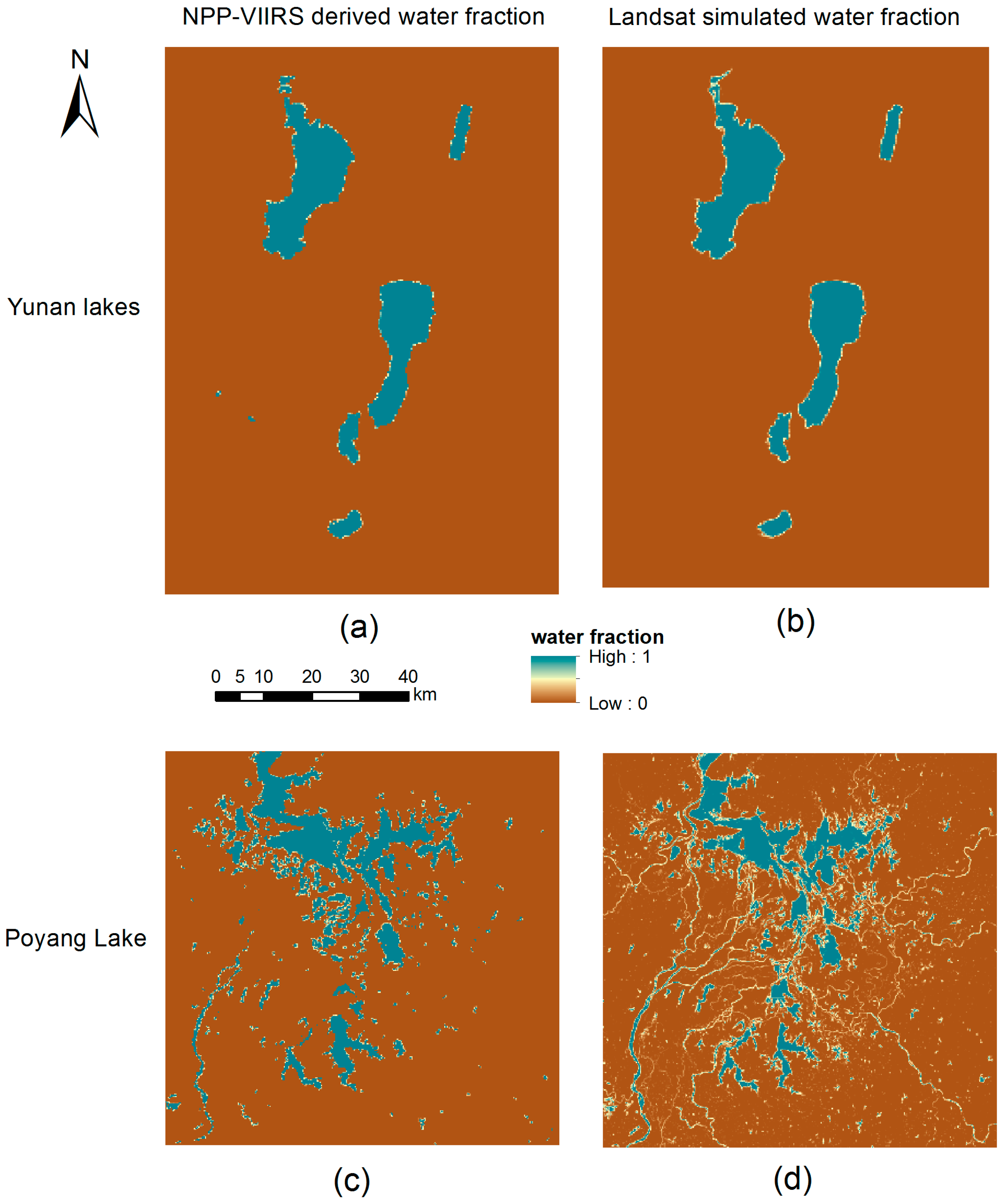
Accuracy assessment in this study includes two aspects, evaluating the accuracy of the water fraction estimation and evaluating the accuracy of subpixel mapping. For both aspects, the referencing data are water cover information derived from corresponding Landsat images. Since Landsat has a much finer resolution than NPP–VIIRS, all Landsat pixels were considered as pure pixels here. A binary water/land classification can be generated using a threshold to the SWIR band (band 6) of the Landsat image [22]. Reflectance values of this band equal to or below the threshold were assigned to water, while those above were classified as land. It can be noted that the threshold must be determined very carefully, because the optimal threshold differs from case to case. In this study, the thresholds were adjusted carefully for each case study with the aid of visual interpretation. For the Yunnan lakes especially, pixels that are far away from the lakes were manually excluded. Binary lake maps with a value of 1 as the lake-water area and 0 as the land were derived, which were then resampled to 15 m resolution using the nearest neighbor method. Landsat-simulated water fraction maps (e.g., Figure 4c,d) were then generated by aggregating the 15 m Landsat lake map to 375 m resolution with a scale factor of 25. Each pixel of these maps maintains the water percentage within its 375 m × 375 m area. These fraction maps were used as the reference to evaluate the accuracy of fraction maps derived from the 375 m resolution NPP–VIIRS. Evaluation was first based on a pixel-by-pixel fraction difference, since they have exactly the same resolution.
Another easy way to validate water fraction results is to compare the satellite-observed lake areas calculated from both estimated and referenced water fraction maps using the following equation [51]:
where fwi is the water fraction of pixel i; si is the area of pixel i; and n stands for the total number of pixels that comprise the lake.
A generalized cross-tabulation matrix (CTM) was proposed by Pontius and Cheuk [52] to evaluate soft classified maps at multiple resolutions. On the basis of CTM, Silván-Cárdenas and Wang [53] developed a subpixel confusion–uncertainty matrix (SCM) to assess sub-pixel mapping accuracy and uncertainties. Compared to the traditional evaluation methods, such as root mean square error (RMSE), SCM is able to provide detailed information on subpixel confusion and uncertainty. It was, therefore, also adopted in this study to evaluate the water fraction estimation results. Accuracy–uncertainty indices were calculated from traditional indices such as overall accuracy and the Kappa coefficient, based on SCM.
Landsat-simulated water fraction maps were also used for subpixel mapping, which provides a comparison for the subpixel mapping results of the NPP–VIIRS-derived water fraction. Subpixel mapping results of both data sources (Landsat-simulated and NPP–VIIRS-derived) were evaluated using the initial resampled 15 m resolution water maps as references. Validation maps were produced by overlaying the subpixel mapping results with reference maps pixel-by-pixel. Some accuracy indices, such as the commission and omission errors, overall accuracy and Kappa coefficient, were calculated from these validation maps to provide an intuitive assessment of the accuracy.
3. Results and Discussion
3.1. Water Fraction Map and Its Accuracy
The I3 bands of the Suomi NPP–VIIRS images as listed in Table 1 were employed as the input of the water fraction retrieval method. Water fraction maps at a spatial resolution of 375 m were then derived (e.g., Figure 4a,c). Corresponding Landsat-simulated water fraction maps (e.g., Figure 4b,d) are displayed for reference.
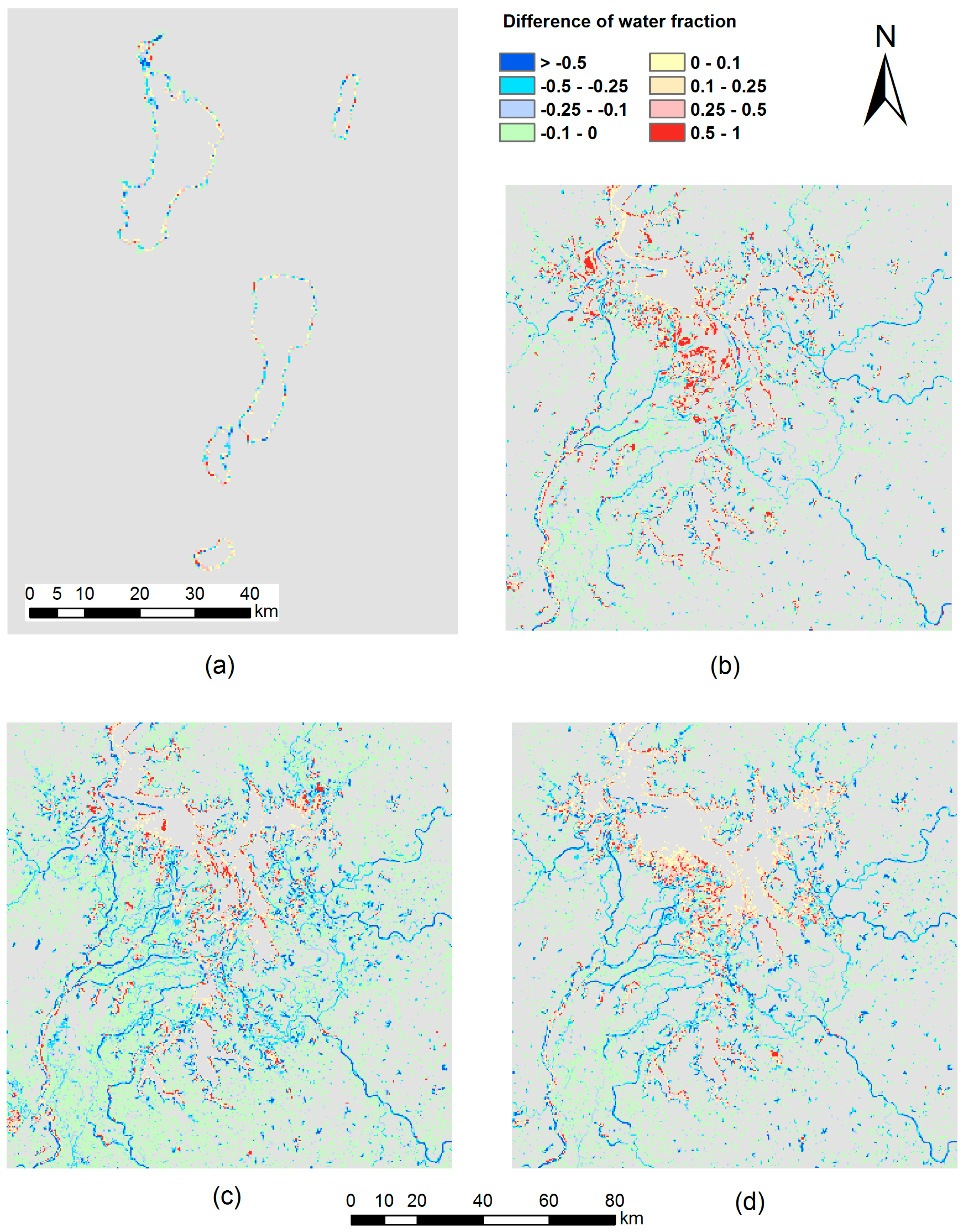
In order to quantify the accuracy of the NPP–VIIRS retrieved water fraction, the corresponding Landsat-simulated water fraction map was employed as the reference. Two maps were overlaid pixel by pixel, generating a difference map as shown in Figure 5. A difference value greater than 0 indicates that water fraction has been overestimated by the NPP–VIIRS image. From Figure 5, the water fraction for Yunnan lakes was slightly underestimated by the NPP–VIIRS in general, because a substantial proportion of pixels have fraction difference values smaller than 0. For Poyang Lake, overestimation is much more common, especially for the result of 5 October 2013 (T1). Underestimation also exists, but mainly occurs in the river channels.
The absolute difference was divided into four levels, less than 0.10, 0.10–0.25, 0.25–0.50, and greater than 0.50. The percentage of pixels that belonged to each level was counted in Table 2. It is clear that most of the pixels have been estimated properly. For the Yunnan lakes, about 66% of the pixels have an absolute difference of less than 0.25. There are only 10% mixed pixels that have an absolute difference greater than 0.5. For all the three cases of Poyang Lake, over 50% mixed pixels have an absolute difference of less than 0.10. There are also about 10% of the mixed pixels whose water fraction has been estimated improperly, with an absolute difference greater than 0.50. This indicates that the water fraction has been retrieved from the NPP–VIIRS image with acceptable accuracy in general, bearing in mind that deviations still exist, some of them are even significant.
The areas of these lakes were calculated using Equation (3) from the NPP–VIIRS-derived and Landsat-simulated fraction maps, respectively (Table 3). Note that for the Poyang Lake cases, the lake area here refers to the total water area in the whole study area. It is obvious that the areas of all the lakes have been estimated properly by the NPP–VIIRS. Qilu Lake has the highest estimation difference, which is about 5%, mainly due to its relatively smaller lake-water area and intricate water body. The area of Poyang Lake varies at three selected dates, which has been captured successfully by both the NPP–VIIRS and Landsat. Estimation for T2 (1 May 2014) has the highest difference (more than 7%) among all three. Based on these results, downscaling the NPP–VIIRS image is proved to be able to achieve generally accurate lake-water coverage estimation.
Accuracy–uncertainty indices, including producer accuracy, user accuracy, overall accuracy and the Kappa coefficient, were calculated based on SCM for lakes in each case study (Table 4). From Table 4, center values of traditional accuracy indices demonstrate the baseline of the accuracy for lakes in each case study. It is found that although the overall accuracy for all the lakes is over 90%, the producer accuracy (PA), user accuracy (UA) and Kappa coefficient are quite different. Dianchi Lake, Yangzonghai Lake and Fuxian Lake in the Yunnan lakes case study have relatively higher accuracy than the others. Corresponding uncertainties for these indices were appended as plus–minus values behind each index. It is found that uncertainties for most of these indices are around 1–2%. Uncertainties for the Kappa coefficient are generally less than 0.03. It is noted that the larger the uncertainty of an index, the less useful the center value will be. In general, the water fractions of lakes for all the case studies have been estimated properly, with some of the Yunnan lakes having relatively higher accuracy and fewer uncertainties.
3.2. Subpixel Mapping Results and Their Accuracy
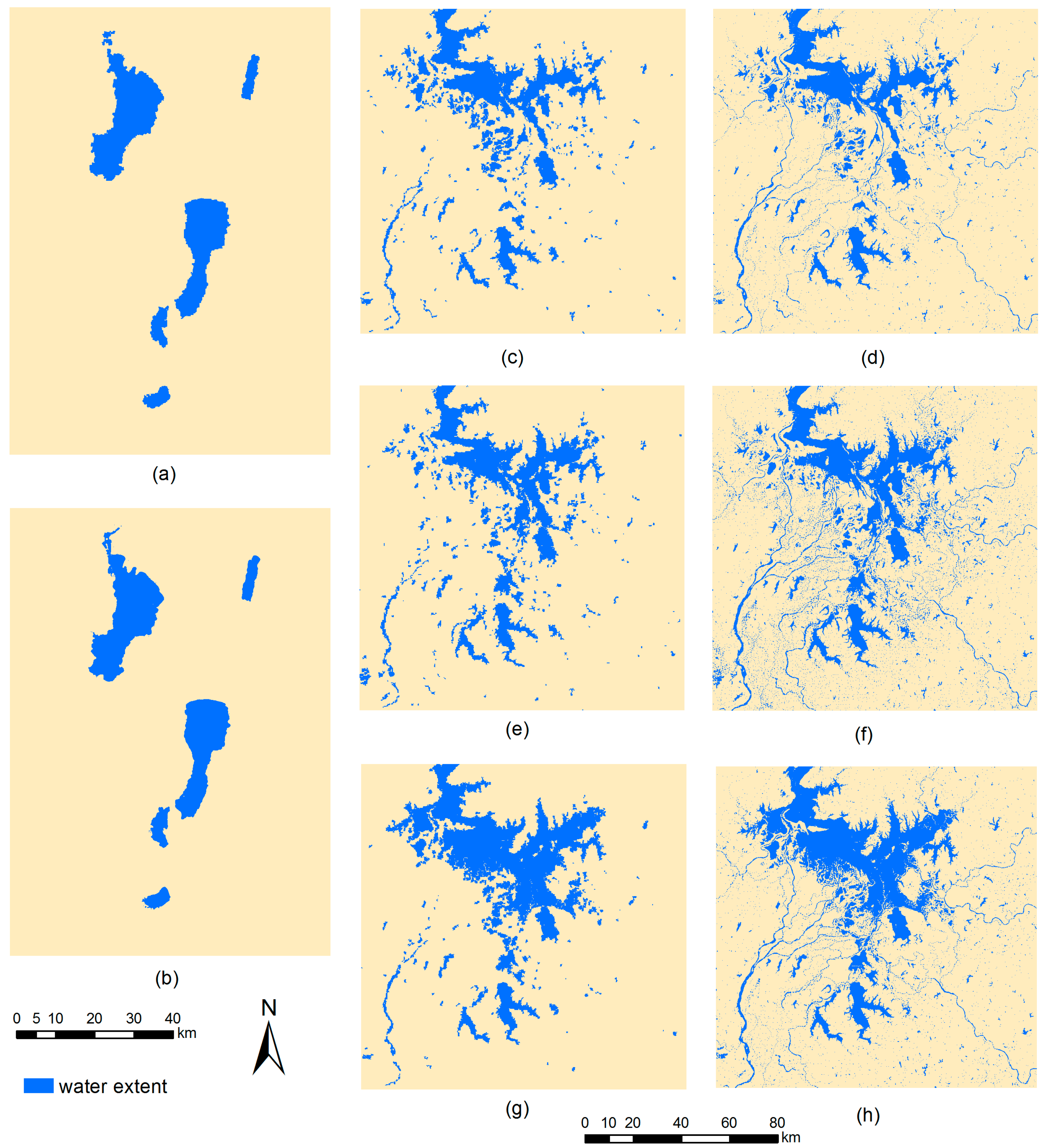
Both the NPP–VIIRS-derived water fraction map (e.g., Figure 4a,c) and the Landsat-simulated water fraction map (e.g., Figure 4b,d) were employed as the input of a subpixel mapping algorithm with a scale factor of 25, respectively. The other parameters of the SPM algorithm, such as the moving window size (r) and exponential parameter of the distance-decay model (α), were adjusted and determined carefully through a series of experiments. Ultimately, the window size was set to 13 and the exponential parameter was given an optimal value of 10 for all cases. With these parameters, downscaled lake maps at a spatial resolution of 15 m were produced and are presented in Figure 6.
It can be observed from Figure 6a that the overall shapes of five Yunnan lakes have been generated appropriately by subpixel mapping the NPP–VIIRS-derived water fraction map. Some subtle parts of the shorelines can even be restored. However, it has also been noted that the downscaled lake shorelines are not as smooth as the actual shorelines portrayed by the Landsat image (Figure 1a). Some delicate areas, such as the inner lake on the north of Dianchi Lake and the wetland on the south-west of Qilu Lake, have not been mapped reasonably. The boundaries of these areas are obviously incorrect compared with those observed from the Landsat image; while the subpixel mapping result of the Landsat-simulated water fraction map (Figure 6b) looks reasonable. The shorelines of all lakes were properly restored, even in the intricate areas.
For Poyang Lake at three different times, the subpixel mapping results of the NPP–VIIRS (Figure 6c,e,g) look inferior to that of the Yunnan lakes, due to its much more complicated shoreline, as well as its rich and small river tributaries. The main lake bodies were retrieved appropriately, but small patches, as well as rivers, were failed to be restored. Nevertheless, the subpixel mapping results of the Landsat-simulated water fraction (Figure 6d,f,h) appear to be much more reasonable. The main lake bodies, small patches and even some small rivers were properly derived.
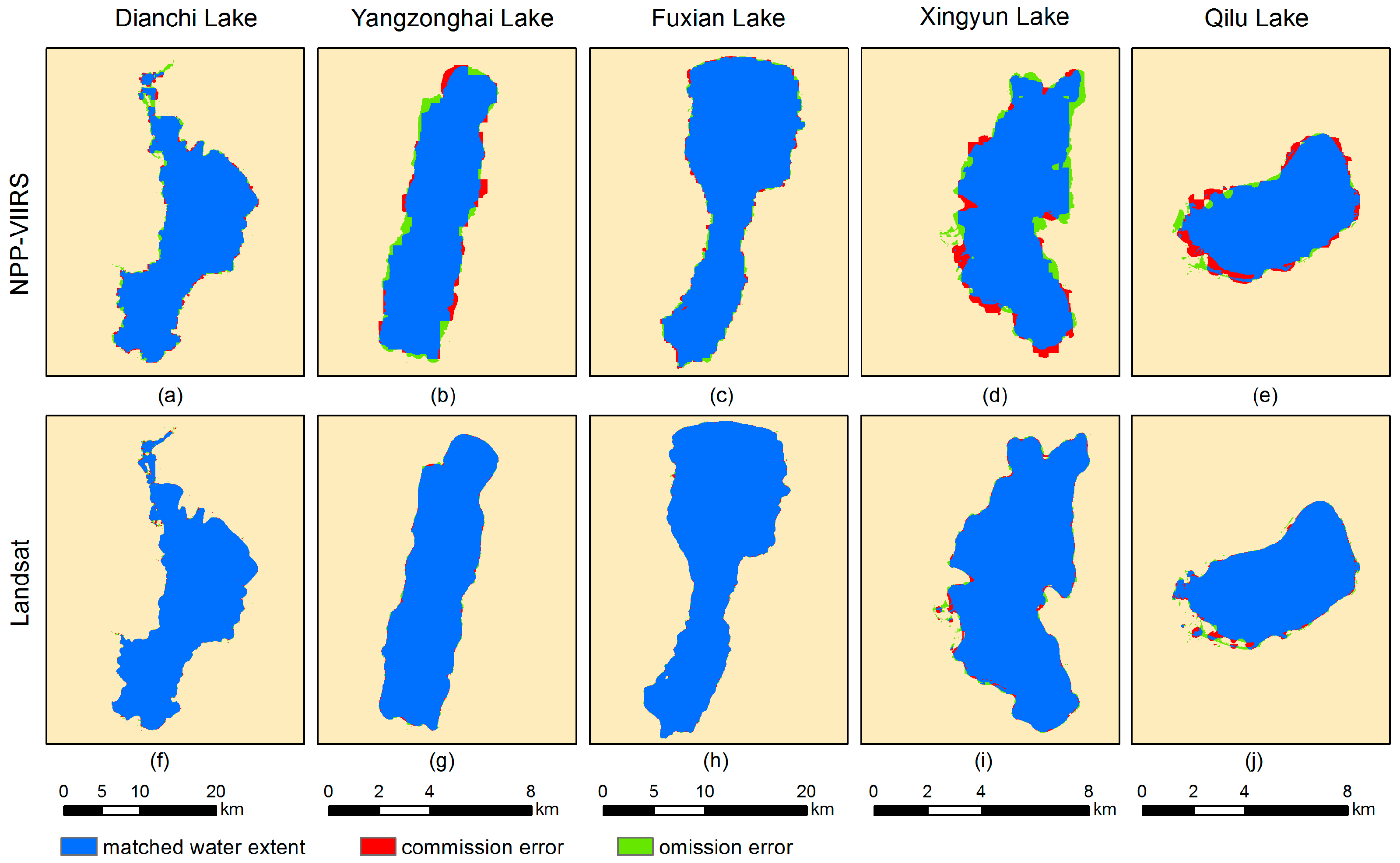
All subpixel mapping results in Figure 6 were overlaid pixel-by-pixel with the corresponding referencing water maps that were derived directly from Landsat images to achieve a quantitative accuracy assessment. The validation maps of the Yunnan lakes are shown in Figure 7. For a better visual effect, five Yunnan lakes were split into separated map frames with different scales. Commission and omission errors can be identified directly from Figure 7. It is clear that errors mainly occur in those parts where the lakes have relatively delicate shorelines. This is even obvious in the NPP–VIIRS derived results (Figure 7a–e). Significant omission errors (green), as well as commission errors (red) occur in the northern part of Dianchi Lake, and also in the south-west boundary of Qilu Lake, while the results that are derived from the Landsat-simulated water fraction (Figure 7f–j) have much higher accuracy, apparently. Even in some intricate areas, errors are very limited. Only some tiny and delicate water areas, for example the small tributaries on the south-west of Qilu Lake and tributaries on the west of Xingyun Lake, have obvious errors.
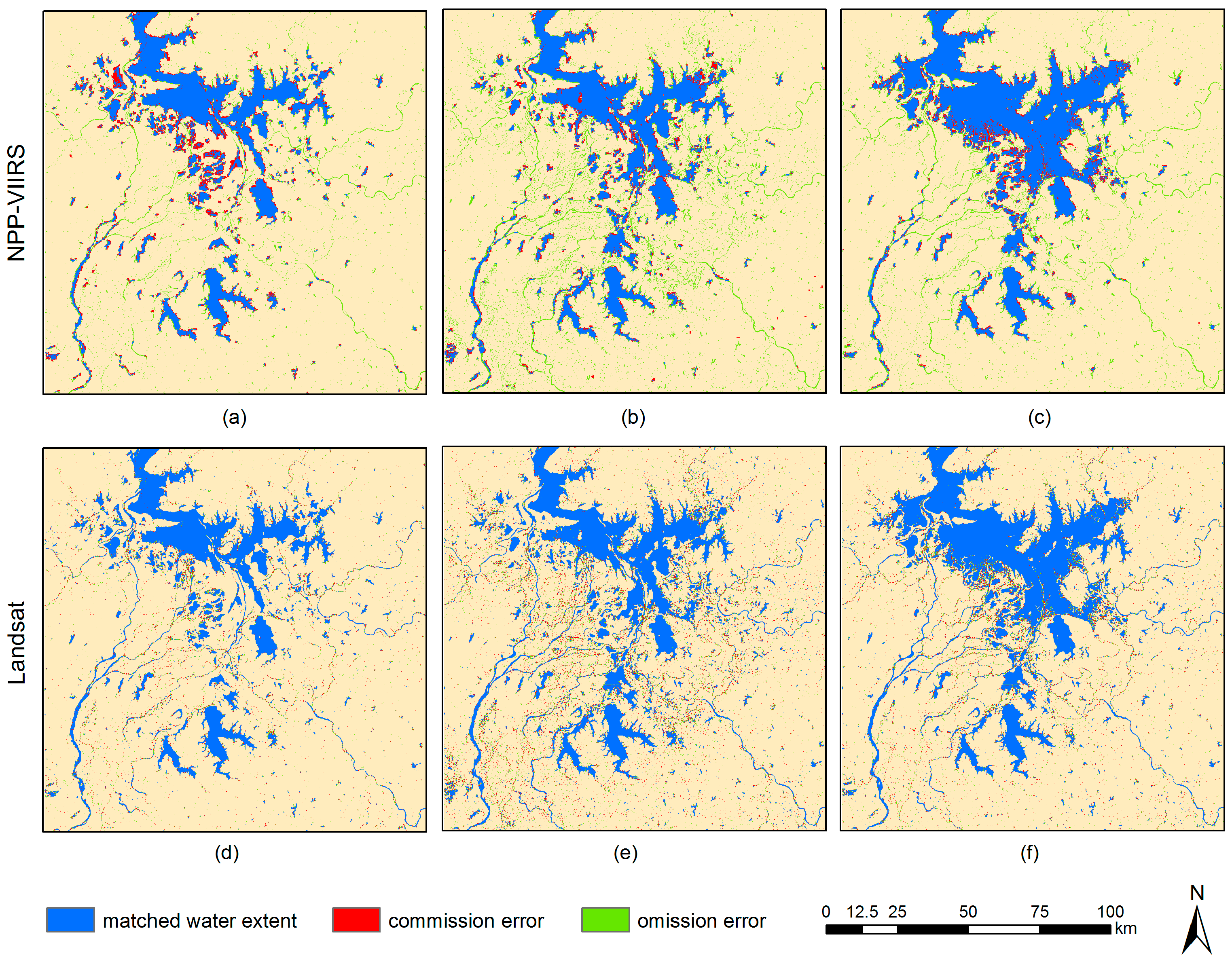
The validation maps of Poyang Lake in Figure 8 reveal that the main lake body has been retrieved correctly at all three times. It is also noted that errors exist substantially in the downscaling results of the NPP–VIIRS data. Commission errors (red) occur mainly in the isolated patches that were formed when the water level dropped in the dry season, while omissions (green) generally happen in narrow river channels. It seems that those fine water bodies cannot be correctly retrieved by downscaling the NPP–VIIRS. On the contrary, the downscaling results of simulated Landsat data have very limited errors, either commission or omission, and even some small rivers can be restored properly.
Percentage of errors, as well as overall accuracy and Kappa coefficient, were calculated based on the overlaying maps. As suggested by Mertens et al. [32], a mask was applied to exclude all pure pixels from the water fraction map in order to achieve a more precise accuracy assessment. These indices were calculated for each lake individually and listed in Table 5.
It is obvious from Table 5 that the accuracy of downscaled maps differs across lakes, dates, and data sources. Lakes downscaled from the Landsat-simulated water fraction maps have many fewer errors than those derived from the NPP–VIIRS water fraction maps. For all the five Yunnan lakes individually, high accuracy has been achieved using the Landsat-simulated water fraction map. Even the worst one, Qilu Lake, has an overall accuracy of 91.32% and a Kappa coefficient of 0.82, which represent a close-to-perfect agreement according to Landis and Koch [54]. While using the NPP–VIIRS-retrieved water fraction map, the downscaling results for the Yunnan lakes have relatively lower accuracy. Dianchi Lake has the highest accuracy, with an overall accuracy of 80.50%, a commission error of 6.81%, and an omission error of 12.69%. Its Kappa coefficient is 0.61 which, according to Landis and Koch [54], is a medium above agreement. The accuracy of the other lakes is a little bit lower than that of Dianchi Lake, indicating that the method of downscaling NPP–VIIRS for lake-water mapping is applicable for the Yunnan lakes, but still needs to be improved. For the three cases of Poyang Lake, bearing in mind that the water bodies are much more complicated, the downscaling results have lower accuracy than those of Yunnan lakes. The downscaling results of the NPP–VIIRS have overall accuracy about 80%, with generally more than 10% omission errors. These errors are largely due to the failure of restoring fine river channels, as shown in Figure 8a–c. When using simulated Landsat, the overall accuracy reaches around 88% for all cases, and the Kappa coefficients are between 0.62 and 0.69. The Poyang Lake cases also suggest that the downscaling method is applicable but imperfect. The accuracy comparison between different downscaling data sources in Table 5 reveals the uncertainties introduced only by fraction errors. It is therefore suggested that water fraction estimation errors, even if sometimes limited (see Table 4), would affect the final downscaling results significantly.
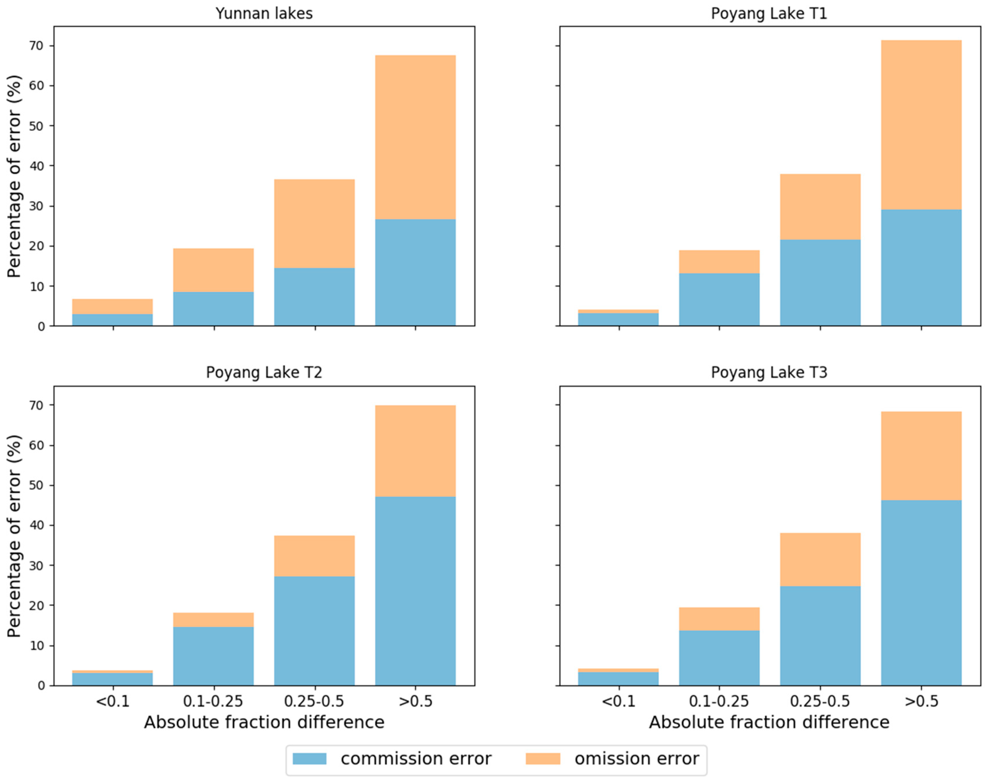
Based on the four levels of absolute fraction difference in Table 2, the NPP–VIIRS mixed pixels were divided into four groups. For each group, percentages of commission and omission errors in the subpixel mapping result were recalculated through dividing the error pixel numbers by total pixel numbers. These percentages of errors for all the four case studies have been displayed as bar charts in Figure 9. It is obvious that as the absolute fraction difference increases, which means the water fraction estimation accuracy decreases, the percentage of commission and omission errors increases significantly, from less than 5% to nearly 70%. This demonstrates that the water fraction estimation results affect the subpixel mapping results seriously.
4. Conclusions
Due to their fine temporal resolution and wide spatial coverage, Suomi NPP–VIIRS data have begun to show their value in surface water and lake-water detection. However, the effective and wide application of this data source is still challenging because of its medium to coarse spatial resolution [21]. The mixed pixel issue seriously affects the accurate detection of land cover, which includes the mapping of lake shorelines. This study has demonstrated the potential of downscaling the 375 m Suomi NPP–VIIRS SWIR band for lake-water area extraction. The purpose is to devise an effective method that improves the spatial resolution as well as the mapping accuracy by combining the spectral unmixing method and subpixel mapping method.
For spectral unmixing, a low-cost, easy-to-implement method was proposed to automatically extract endmembers from the image for estimating water fraction based on the principle of the linear spectral mixture model. An accurate and globally available water dynamic dataset was employed to automatically refine the feasible value ranges of pure water and pure land reflectance, which helps avoid uncertainties introduced by human intervention. Through either lake area comparison or the subpixel confusion–uncertainty matrix, it was proved that the water fraction had been properly estimated from the NPP–VIIRS. By directly comparing this with the referencing fraction map, a limited proportion of pixels was found to have large fraction deviations (greater than 0.50). However, it is also noted that water and land endmembers acquired with the proposed method are sometimes unable to reflect the real land cover types in the study area precisely, especially for the land endmember, because the non-water land cover type varies from place to place. The reflectance of these land cover types is also quite different from others. It is almost impossible to select a single endmember to represent all non-water land covers exactly, although the moving window approach does make the selected endmembers more representative to some extent.
When subpixel mapping a lake area, it would be helpful to make some modifications to the traditional subpixel mapping algorithms, such as modifications to the random initialization and attractiveness calculation, since the location of main lake body is easily acquired from the water product involved. These modifications would enhance the subpixel mapping algorithms by either reducing the calculation or improving the final result.
It is demonstrated that by downscaling NPP–VIIRS data using the proposed two-step process, lake maps at finer resolution can be generated with proper accuracy. This methodology could also be easily applied to other similar sensors such as MODIS. This could be useful because these coarse resolution data usually have fine temporal resolution, which means they are usually available while other finer spatial resolution data are not. Spatial downscaling these data produces lake maps with finer spatial resolution and higher accuracy compared to their hard classification results. Daily lake water products at fine spatial resolutions could be produced from daily MODIS or NPP–VIIRS time-series using the downscaling method, bearing in mind that uncertainties may be introduced by the downscaling process. It also has to be noted that while having all these advantages, the downscaling process sometimes requires intensive additional computation.
Based on the downscaling results of both the NPP–VIIRS-derived and Landsat-simulated water fraction maps, it has been found that the water fraction retrieval process introduced more uncertainties and errors into the final result than the subpixel mapping process. The subpixel mapping result of the Landsat-simulated water fraction map that has the exact water fraction values entails very limited errors, while the downscaling fraction map that is derived from the actual NPP–VIIRS image produced much more errors, although the validation results reveal that the NPP–VIIRS-derived water fraction has acceptable accuracy. Only a small proportion of the pixels have fraction deviations greater than 0.50. Most of the estimated water fractions have deviations smaller than that. However, it seems that these deviations, even though sometimes small, may still affect subpixel mapping results. This is because the spatial allocation of water subpixels is based on the water fraction within each coarse mixed pixel. When the fraction is not accurate, it is difficult for any type of optimal method to restore the correct subpixel mapping results. On the contrary, if the water fraction was retrieved correctly, the shoreline of lakes could be easily restored at the subpixel scale with high accuracy. It is therefore suggested that future work on downscale lake mapping should focus more on improving the unmixing procedure. It is hoped that this study could promote the application of some moderate resolution sensors, such as the Suomi NPP–VIIRS and MODIS, in monitoring lake-water areas. It is anticipated that in the near future, after the downscaling method has been significantly improved, a daily lake-water product at fine spatial resolutions could be generated from time-series MODIS and NPP–VIIRS data.
Acknowledgments
This is an extended work of a conference paper that was presented at the 1st International Electronic Conference on Water Science. This work was supported by the National Key Research and Development Plan (2017YFC0404302) and Natural Science Foundation of China (41501460, 41671056, and 41601353). We would like to thank Tingbao Xu for his help in initially reviewing this paper. Furthermore, we highly appreciate valuable and constructive comments on the manuscript provided by the anonymous reviewers.
Author Contributions
Chang Huang, Yun Chen and Shiqiang Zhang contributed the main idea and designed the experiments; Linyi Li performed the experiments; Kaifang Shi and Rui Liu analyzed the remote sensing data; and Chang Huang wrote the manuscript, which was then improved by the contribution of all the co-authors.
Conflicts of Interest
The authors declare no conflict of interest.
References
- Singh, A.; Seitz, F.; Schwatke, C. Inter-annual water storage changes in the Aral Sea from multi-mission satellite altimetry, optical remote sensing, and GRACE satellite gravimetry. Remote Sens. Environ. 2012, 123, 187–195. [Google Scholar] [CrossRef]
- Lee, H.; Durand, M.; Jung, H.C.; Alsdorf, D.; Shum, C.K.; Sheng, Y. Characterization of surface water storage changes in arctic lakes using simulated SWOT measurements. Int. J. Remote Sens. 2010, 31, 3931–3953. [Google Scholar] [CrossRef]
- Haas, E.M.; Bartholomé, E.; Lambin, E.F.; Vanacker, V. Remotely sensed surface water extent as an indicator of short-term changes in ecohydrological processes in sub-Saharan Western Africa. Remote Sens. Environ. 2011, 115, 3436–3445. [Google Scholar] [CrossRef]
- Huang, S.; Dahal, D.; Young, C.; Chander, G.; Liu, S. Integration of palmer drought severity index and remote sensing data to simulate wetland water surface from 1910 to 2009 in Cottonwood Lake area, North Dakota. Remote Sens. Environ. 2011, 115, 3377–3389. [Google Scholar] [CrossRef]
- McCullough, I.M.; Loftin, C.S.; Sader, S.A. Combining lake and watershed characteristics with Landsat TM data for remote estimation of regional lake clarity. Remote Sens. Environ. 2012, 123, 109–115. [Google Scholar] [CrossRef]
- Ding, X.W.; Li, X.F. Monitoring of the water-area variations of Lake Dongting in China with ENVISAT ASAR images. Int. J. Appl. Earth Obs. Geoinf. 2011, 13, 894–901. [Google Scholar] [CrossRef]
- Zeng, L.; Schmitt, M.; Li, L.; Zhu, X.X. Analysing changes of the Poyang Lake water area using Sentinel-1 synthetic aperture radar imagery. Int. J. Remote Sens. 2017, 38, 7041–7069. [Google Scholar] [CrossRef]
- Huang, C.; Nguyen, B.D.; Zhang, S.Q.; Cao, S.M.; Wagner, W. A Comparison of Terrain Indices toward Their Ability in Assisting Surface Water Mapping from Sentinel-1 Data. ISPRS Int. J. Geo-Inf. 2017, 6, 140. [Google Scholar] [CrossRef]
- Frazier, P.S.; Page, K.J. Water body detection and delineation with Landsat TM data. Photogramm. Eng. Remote Sens. 2000, 66, 1461–1467. [Google Scholar]
- Chen, Y.; Wang, B.; Pollino, C.A.; Cuddy, S.M.; Merrin, L.E.; Huang, C. Estimate of flood inundation and retention on wetlands using remote sensing and GIS. Ecohydrology 2014, 7, 1412–1420. [Google Scholar] [CrossRef]
- Du, Z.; Li, W.; Zhou, D.; Tian, L.; Ling, F.; Wang, H.; Gui, Y.; Sun, B. Analysis of Landsat-8 OLI imagery for land surface water mapping. Remote Sens. Lett. 2014, 5, 672–681. [Google Scholar] [CrossRef]
- Sheng, Y.; Gong, P.; Xiao, Q. Quantitative dynamic flood monitoring with NOAA AVHRR. Int. J. Remote Sens. 2001, 22, 1709–1724. [Google Scholar] [CrossRef]
- Barton, I.J.; Bathols, J.M. Monitoring floods with AVHRR. Remote Sens. Environ. 1989, 30, 89–94. [Google Scholar] [CrossRef]
- Chen, Y.; Huang, C.; Ticehurst, C.; Merrin, L.; Thew, P. An evaluation of MODIS daily and 8-day composite products for floodplain and wetland inundation mapping. Wetlands 2013, 33, 823–835. [Google Scholar] [CrossRef]
- Huang, C.; Chen, Y.; Wu, J. Mapping spatio-temporal flood inundation dynamics at large river basin scale using time-series flow data and MODIS imagery. Int. J. Appl. Earth Obs. Geoinf. 2014, 26, 350–362. [Google Scholar] [CrossRef]
- Feng, L.; Hu, C.M.; Chen, X.L.; Cai, X.B.; Tian, L.Q.; Gan, W.X. Assessment of inundation changes of Poyang Lake using MODIS observations between 2000 and 2010. Remote Sens. Environ. 2012, 121, 80–92. [Google Scholar] [CrossRef]
- Xu, H.Q. Modification of normalised difference water index (NDWI) to enhance open water features in remotely sensed imagery. Int. J. Remote Sens. 2006, 27, 3025–3033. [Google Scholar] [CrossRef]
- Li, S.; Sun, D.; Yu, Y.; Csiszar, I.; Stefanidis, A.; Goldberg, M.D. A new short-wave infrared (SWIR) method for quantitative water fraction derivation and evaluation with EOS/MODIS and Landsat/TM data. IEEE Trans. Geosci. Remote Sens. 2013, 51, 1852–1862. [Google Scholar] [CrossRef]
- Shi, K.; Huang, C.; Yu, B.; Yin, B.; Huang, Y.; Wu, J. Evaluation of NPP-VIIRS night-time light composite data for extracting built-up urban areas. Remote Sens. Lett. 2014, 5, 358–366. [Google Scholar] [CrossRef]
- Yu, Y.; Privette, J.L.; Pinheiro, A.C. Analysis of the NPOESS VIIRS land surface temperature algorithm using MODIS data. IEEE Trans. Geosci. Remote Sens. 2005, 43, 2340–2350. [Google Scholar]
- Huang, C.; Chen, Y.; Wu, J.; Li, L.; Liu, R. An evaluation of Suomi NPP-VIIRS data for surface water detection. Remote Sens. Lett. 2015, 6, 155–164. [Google Scholar] [CrossRef]
- Olthof, I.; Fraser, R.H.; Schmitt, C. Landsat-based mapping of thermokarst lake dynamics on the Tuktoyaktuk Coastal Plain, Northwest Territories, Canada since 1985. Remote Sens. Environ. 2015, 168, 194–204. [Google Scholar] [CrossRef]
- Mueller, N.; Lewis, A.; Roberts, D.; Ring, S.; Melrose, R.; Sixsmith, J.; Lymburner, L.; McIntyre, A.; Tan, P.; Curnow, S.; et al. Water observations from space: Mapping surface water from 25 years of Landsat imagery across Australia. Remote Sens. Environ. 2016, 174, 341–352. [Google Scholar] [CrossRef]
- Pekel, J.-F.; Cottam, A.; Gorelick, N.; Belward, A.S. High-resolution mapping of global surface water and its long-term changes. Nature 2016, 540, 418–422. [Google Scholar] [CrossRef] [PubMed]
- Donchyts, G.; Baart, F.; Winsemius, H.; Gorelick, N.; Kwadijk, J.; van de Giesen, N. Earth’s surface water change over the past 30 years. Nat. Clim. Chang. 2016, 6, 810–813. [Google Scholar] [CrossRef]
- Yamazaki, D.; Trigg, M.A. Hydrology: The dynamics of earth’s surface water. Nature 2016, 540, 348–349. [Google Scholar] [CrossRef] [PubMed]
- Keshava, N.; Mustard, J.F. Spectral unmixing. IEEE Signal Process. Mag. 2002, 19, 44–57. [Google Scholar] [CrossRef]
- Keshava, N. A survey of spectral unmixing algorithms. Linc. Lab. J. 2003, 14, 55–78. [Google Scholar]
- Ma, B.; Wu, L.; Zhang, X.; Li, X.; Liu, Y.; Wang, S. Locally adaptive unmixing method for lake-water area extraction based on MODIS 250m bands. Int. J. Appl. Earth Obs. Geoinf. 2014, 33, 109–118. [Google Scholar] [CrossRef]
- Atkinson, P.M.; Cutler, M.E.J.; Lewis, H. Mapping sub-pixel proportional land cover with AVHRR imagery. Int. J. Remote Sens. 1997, 18, 917–935. [Google Scholar] [CrossRef]
- Tatem, A.J.; Lewis, H.G.; Atkinson, P.M.; Nixon, M.S. Super-resolution land cover pattern prediction using a hopfield neural network. Remote Sens. Environ. 2002, 79, 1–14. [Google Scholar] [CrossRef]
- Mertens, K.C.; Verbeke, L.P.C.; Ducheyne, E.I.; De Wulf, R.R. Using genetic algorithms in sub-pixel mapping. Int. J. Remote Sens. 2003, 24, 4241–4247. [Google Scholar] [CrossRef]
- Li, L.; Chen, Y.; Xu, T.; Liu, R.; Shi, K.; Huang, C. Super-resolution mapping of wetland inundation from remote sensing imagery based on integration of back-propagation neural network and genetic algorithm. Remote Sens. Environ. 2015, 164, 142–154. [Google Scholar] [CrossRef]
- Mertens, K.C.; De Baets, B.; Verbeke, L.P.C.; De Wulf, R.R. A sub-pixel mapping algorithm based on sub-pixel/pixel spatial attraction models. Int. J. Remote Sens. 2006, 27, 3293–3310. [Google Scholar] [CrossRef]
- Ling, F.; Li, X.D.; Du, Y.; Xiao, F. Sub-pixel mapping of remotely sensed imagery with hybrid intra- and inter-pixel dependence. Int. J. Remote Sens. 2013, 34, 341–357. [Google Scholar] [CrossRef]
- Ling, F.; Du, Y.; Xiao, F.; Xue, H.P.; Wu, S.J. Super-resolution land-cover mapping using multiple sub-pixel shifted remotely sensed images. Int. J. Remote Sens. 2010, 31, 5023–5040. [Google Scholar] [CrossRef]
- Atkinson, P.M. Sub-pixel target mapping from soft-classified, remotely sensed imagery. Photogramm. Eng. Remote Sens. 2005, 71, 839–846. [Google Scholar] [CrossRef]
- Thornton, M.W.; Atkinson, P.M.; Holland, D.A. A linearised pixel-swapping method for mapping rural linear land cover features from fine spatial resolution remotely sensed imagery. Comput. Geosci. 2007, 33, 1261–1272. [Google Scholar] [CrossRef]
- Huang, C.; Chen, Y.; Wu, J.P. Dem-based modification of pixel-swapping algorithm for enhancing floodplain inundation mapping. Int. J. Remote Sens. 2014, 35, 365–381. [Google Scholar] [CrossRef]
- Ling, F.; Fang, S.; Li, W.; Li, X.; Xiao, F.; Zhang, Y.; Du, Y. Post-processing of interpolation-based super-resolution mapping with morphological filtering and fraction refilling. Int. J. Remote Sens. 2014, 35, 5251–5262. [Google Scholar] [CrossRef]
- Li, L.; Chen, Y.; Yu, X.; Liu, R.; Huang, C. Sub-pixel flood inundation mapping from multispectral remotely sensed images based on discrete particle swarm optimization. ISPRS J. Photogramm. Remote Sens. 2015, 101, 10–21. [Google Scholar] [CrossRef]
- Foody, G.M.; Muslim, A.M.; Atkinson, P.M. Super-resolution mapping of the waterline from remotely sensed data. Int. J. Remote Sens. 2005, 26, 5381–5392. [Google Scholar] [CrossRef]
- Ling, F.; Xiao, F.; Du, Y.; Xue, H.P.; Ren, X.Y. Waterline mapping at the subpixel scale from remote sensing imagery with high-resolution digital elevation models. Int. J. Remote Sens. 2008, 29, 1809–1815. [Google Scholar] [CrossRef]
- Muslim, A.M.; Foody, G.M.; Atkinson, P.M. Localized soft classification for super-resolution mapping of the shoreline. Int. J. Remote Sens. 2006, 27, 2271–2285. [Google Scholar] [CrossRef]
- Muad, A.M.; Foody, G.M. Super-resolution mapping of lakes from imagery with a coarse spatial and fine temporal resolution. Int. J. Appl. Earth Obs. Geoinf. 2012, 15, 79–91. [Google Scholar] [CrossRef]
- Shah, C.A. Automated lake shoreline mapping at subpixel accuracy. IEEE Geosci. Remote Sens. Lett. 2011, 8, 1125–1129. [Google Scholar] [CrossRef]
- Pardo-Pascual, J.E.; Almonacid-Caballer, J.; Ruiz, L.A.; Palomar-Vazquez, J. Automatic extraction of shorelines from Landsat TM and ETM+ multi-temporal images with subpixel precision. Remote Sens. Environ. 2012, 123, 1–11. [Google Scholar] [CrossRef]
- Xu, G.; Qin, Z. Flood estimation methods for Poyang Lake area. J. Lake Sci. 1998, 10, 31–36. [Google Scholar]
- Shankman, D.; Keim, B.D.; Song, J. Flood frequency in China’s Poyang Lake region: Trends and teleconnections. Int. J. Climatol. 2006, 26, 1255–1266. [Google Scholar] [CrossRef]
- Haertel, V.F.; Shimabukuro, Y.E. Spectral linear mixing model in low spatial resolution image data. IEEE Trans. Geosci. Remote Sens. 2005, 43, 2555–2562. [Google Scholar] [CrossRef]
- Verdin, J.P. Remote sensing of ephemeral water bodies in western Niger. Int. J. Remote Sens. 1996, 17, 733–748. [Google Scholar] [CrossRef]
- Pontius, R.G., Jr.; Cheuk, M.L. A generalized cross-tabulation matrix to compare soft-classified maps at multiple resolutions. Int. J. Geogr. Inf. Sci. 2006, 20, 1–30. [Google Scholar] [CrossRef]
- Silván-Cárdenas, J.L.; Wang, L. Sub-pixel confusion–uncertainty matrix for assessing soft classifications. Remote Sens. Environ. 2008, 112, 1081–1095. [Google Scholar] [CrossRef]
- Landis, J.R.; Koch, G.G. The measurement of observer agreement for categorical data. Biometrics 1977, 33, 159–174. [Google Scholar] [CrossRef] [PubMed]
Figure 1.
Maps of study areas showing the locations of (a) Yunnan lakes, and (b) Poyang Lake.

Figure 2.
(a) Water extent of Yunnan lakes; (b) water occurrence of Yunnan Lakes; (c) water extent of Poyang Lake; and (d) water occurrence of Poyang Lake, extracted from the global water dynamic dataset published by Pekel et al. [24].
Figure 2.
(a) Water extent of Yunnan lakes; (b) water occurrence of Yunnan Lakes; (c) water extent of Poyang Lake; and (d) water occurrence of Poyang Lake, extracted from the global water dynamic dataset published by Pekel et al. [24].


Figure 3.
An example of the two-peak histogram of the NPP–VIIRS short-wave infrared (SWIR) band, and the demonstration of feasible ranges.
Figure 3.
An example of the two-peak histogram of the NPP–VIIRS short-wave infrared (SWIR) band, and the demonstration of feasible ranges.

Figure 4.
(a) Water fraction map derived from the Suomi NPP–VIIRS I3 band for Yunnan lakes on 2 February 2014; (b) water fraction map derived from Landsat band 6 for Yunnan lakes on 2 February 2014; (c) water fraction map derived from Suomi NPP–VIIRS I3 band for Poyang Lake on 5 October 2013; (d) water fraction map derived from Landsat band 6 for Poyang Lake on 5 October 2013.

Figure 5.
Difference between the NPP–VIIRS water fraction and the Landsat-simulated water fraction for the four case studies in Table 1: (a) Yunnan lakes; (b) Poyang Lake T1; (c) Poyang Lake T2; (d) Poyang Lake T3.
Figure 5.
Difference between the NPP–VIIRS water fraction and the Landsat-simulated water fraction for the four case studies in Table 1: (a) Yunnan lakes; (b) Poyang Lake T1; (c) Poyang Lake T2; (d) Poyang Lake T3.

Figure 6.
(a) Subpixel mapping result of NPP–VIIRS-derived water fraction for Yunnan lakes on 2 February 2014; (b) subpixel mapping result of Landsat-simulated water fraction for Yunnan lakes on 2 February 2014; (c) subpixel mapping result of NPP–VIIRS-derived water fraction for Poyang Lake on 5 October 2013; (d) subpixel mapping result of Landsat-simulated water fraction for Poyang Lake on 5 October 2013; (e) subpixel mapping result of NPP–VIIRS-derived water fraction for Poyang Lake on 1 May 2014; (f) subpixel mapping result of Landsat-simulated water fraction for Poyang Lake on 1 May 2014; (g) subpixel mapping result of NPP–VIIRS-derived water fraction for Poyang Lake on 8 October 2014; and (h) subpixel mapping result of Landsat-simulated water fraction for Poyang Lake on 8 October 2014.

Figure 7.
Validation results of subpixel mapping of: (a) Dianchi Lake from the NPP–VIIRS; (b) Yangzonghai Lake from the NPP–VIIRS; (c) Fuxian Lake from the NPP–VIIRS; (d) Xingyun Lake from the NPP–VIIRS; (e) Qilu Lake from the NPP–VIIRS; (f) Dianchi Lake from the Landsat; (g) Yangzonghai Lake from the Landsat; (h) Fuxian Lake from the Landsat; (i) Xingyun Lake from the Landsat; and (j) Qilu Lake from the Landsat.

Figure 8.
Validation results of subpixel mapping of Poyang Lake (a) from the NPP–VIIRS on 5 October 2013; (b) from the NPP–VIIRS on 1 May 2014; (c) from the NPP–VIIRS on 8 October 2014; (d) from the Landsat on 5 October 2013; (e) from the Landsat on 1 May 2014; (f) from the Landsat on 8 October 2014.

Figure 9.
Commission and omission errors of subpixel mapping of mixed pixels with different levels of absolute difference.
Figure 9.
Commission and omission errors of subpixel mapping of mixed pixels with different levels of absolute difference.


Table 1.
Selected case studies and remotely sensed images involved.
| Case Study | Image Type | Image Date | Acquisition Time | Path/Row | Spatial Resolution |
|---|---|---|---|---|---|
| Yunnan lakes | NPP-VIIRS | 2 February 2014 | 06:39:57 | -- | 375 m |
| Landsat OLI | 2 February 2014 | 03:36:02 | 129/43 | 30 m | |
| Poyang Lake T1 | NPP-VIIRS | 5 October 2013 | 05:52:14 | -- | 375 m |
| Landsat OLI | 5 October 2013 | 02:46:14 | 121/40 | 30 m | |
| Poyang Lake T2 | NPP-VIIRS | 1 May 2014 | 05:53:21 | -- | 375 m |
| Landsat OLI | 1 May 2014 | 02:44:05 | 121/40 | 30 m | |
| Poyang Lake T3 | NPP-VIIRS | 8 October 2014 | 05:52:50 | -- | 375 m |
| Landsat OLI | 8 October 2014 | 02:44:32 | 121/40 | 30 m |
Table 2.
Percentage of mixed pixels with four levels of absolute difference.
| Case Study | Percentage of Pixels that Have an Absolute Difference | |||
|---|---|---|---|---|
| <0.10 | 0.10–0.25 | 0.25–0.50 | >0.50 | |
| Yunnan lakes | 39% | 27% | 24% | 10% |
| Poyang Lake T1 | 53% | 19% | 16% | 12% |
| Poyang Lake T2 | 61% | 18% | 13% | 8% |
| Poyang Lake T3 | 54% | 20% | 16% | 10% |
Table 3.
Difference of lake areas * calculated from the NPP–VIIRS and Landsat.
| Case Study | Lake | Lake Area on NPP-VIIRS (km2) | Lake Area on Landsat (km2) | Difference (%) |
|---|---|---|---|---|
| Yunnan lakes | Dianchi Lake | 289.30 | 294.26 | 1.69 |
| Yangzonghai Lake | 28.84 | 29.47 | 2.14 | |
| Fuxian Lake | 212.40 | 213.83 | 0.67 | |
| Xingyun Lake | 31.13 | 31.86 | 2.29 | |
| Qilu Lake | 23.80 | 22.59 | 5.36 | |
| Poyang Lake T1 | Poyang Lake | 2011.32 | 2093.30 | 3.92 |
| Poyang Lake T2 | Poyang Lake | 2107.93 | 2277.45 | 7.44 |
| Poyang Lake T3 | Poyang Lake | 2666.81 | 2766.85 | 3.62 |
Note: * For the Poyang Lake cases, lake area refers to the total water area in the whole study area.
Table 4.
Accuracy assessment of lake-water fraction estimation based on the subpixel confusion–uncertainty matrix (SCM).
Table 4.
Accuracy assessment of lake-water fraction estimation based on the subpixel confusion–uncertainty matrix (SCM).
| Case Study | Lake | Producer Accuracy (%) with Uncertainty | User Accuracy (%) with Uncertainty | Overall Accuracy (%) with Uncertainty | Kappa Coefficient with Uncertainty |
|---|---|---|---|---|---|
| Yunnan lakes | Dianchi Lake | 95.33 ± 1.05 | 96.95 ± 1.09 | 97.94 ± 0.58 | 0.95 ± 0.02 |
| Yangzonghai Lake | 92.09 ± 1.78 | 94.09 ± 1.86 | 98.26 ± 0.48 | 0.92 ± 0.02 | |
| Fuxian Lake | 96.91 ± 0.80 | 97.56 ± 0.81 | 97.94 ± 0.60 | 0.96 ± 0.01 | |
| Xingyun Lake | 90.17 ± 1.92 | 92.22 ± 2.01 | 95.09 ± 1.14 | 0.88 ± 0.03 | |
| Qilu Lake | 93.94 ± 2.52 | 89.29 ± 2.28 | 95.93 ± 1.20 | 0.89 ± 0.03 | |
| Poyang Lake T1 | Poyang Lake | 75.46 ± 1.72 | 78.47 ± 1.86 | 94.70 ± 0.50 | 0.74 ± 0.03 |
| Poyang Lake T2 | Poyang Lake | 63.28 ± 1.27 | 82.88 ± 2.18 | 92.30 ± 0.57 | 0.67 ± 0.03 |
| Poyang Lake T3 | Poyang Lake | 75.70 ± 1.58 | 86.80 ± 2.07 | 93.88 ± 0.67 | 0.77 ± 0.03 |
Table 5.
Accuracy indices showing the evaluation result of different lakes on both the NPP–VIIRS and Landsat downscaling results for different case studies.
Table 5.
Accuracy indices showing the evaluation result of different lakes on both the NPP–VIIRS and Landsat downscaling results for different case studies.
| Case Study | Lake | Downscaling Data Source | Commission Error (%) | Omission Error (%) | Overall Accuracy (%) | Kappa Coefficient |
|---|---|---|---|---|---|---|
| Yunnan lakes | Dianchi Lake | NPP-VIIRS | 6.81 | 12.69 | 80.50 | 0.61 |
| Landsat | 2.86 | 2.83 | 94.31 | 0.89 | ||
| Yangzonghai Lake | NPP-VIIRS | 8.42 | 13.24 | 78.34 | 0.56 | |
| Landsat | 1.59 | 1.56 | 96.85 | 0.97 | ||
| Fuxian Lake | NPP-VIIRS | 8.75 | 12.27 | 78.98 | 0.59 | |
| Landsat | 2.35 | 2.32 | 95.33 | 0.91 | ||
| Xingyun Lake | NPP-VIIRS | 9.95 | 14.62 | 75.43 | 0.51 | |
| Landsat | 2.71 | 2.66 | 94.63 | 0.89 | ||
| Qilu Lake | NPP-VIIRS | 16.25 | 6.61 | 77.14 | 0.55 | |
| Landsat | 4.34 | 4.34 | 91.32 | 0.82 | ||
| Poyang Lake T1 | Poyang Lake | NPP-VIIRS | 9.20 | 11.01 | 79.79 | 0.42 |
| Landsat | 5.43 | 5.43 | 89.14 | 0.69 | ||
| Poyang Lake T2 | Poyang Lake | NPP-VIIRS | 4.13 | 12.02 | 83.85 | 0.48 |
| Landsat | 5.74 | 5.74 | 88.52 | 0.62 | ||
| Poyang Lake T3 | Poyang Lake | NPP-VIIRS | 5.96 | 12.95 | 81.09 | 0.46 |
| Landsat | 6.26 | 6.26 | 87.48 | 0.67 |
© 2017 by the authors. Licensee MDPI, Basel, Switzerland. This article is an open access article distributed under the terms and conditions of the Creative Commons Attribution (CC BY) license (http://creativecommons.org/licenses/by/4.0/).
Share and Cite
MDPI and ACS Style
Huang, C.; Chen, Y.; Zhang, S.; Li, L.; Shi, K.; Liu, R. Spatial Downscaling of Suomi NPP–VIIRS Image for Lake Mapping. Water 2017, 9, 834. https://doi.org/10.3390/w9110834
AMA Style
Huang C, Chen Y, Zhang S, Li L, Shi K, Liu R. Spatial Downscaling of Suomi NPP–VIIRS Image for Lake Mapping. Water. 2017; 9(11):834. https://doi.org/10.3390/w9110834
Chicago/Turabian StyleHuang, Chang, Yun Chen, Shiqiang Zhang, Linyi Li, Kaifang Shi, and Rui Liu. 2017. "Spatial Downscaling of Suomi NPP–VIIRS Image for Lake Mapping" Water 9, no. 11: 834. https://doi.org/10.3390/w9110834
Note that from the first issue of 2016, this journal uses article numbers instead of page numbers. See further details here.