
Abiotic–Biotic Interrelations in the Context of Stabilized Ecological Potential of Post-Mining Waters

1
Department of Ichthyology, Hydrobiology and Aquatic Ecology, National Inland Fisheries Research Institute, Oczapowskiego St. 10, 10-719 Olsztyn, Poland
2
Institute of Engineering and Environmental Protection, Faculty of Geoengineering, University of Warmia and Mazury, Oczapowskiego St. 5, 10-719 Olsztyn, Poland
3
Department of Environmental Protection, Faculty of Geology, Geophysics and Environmental Protection, AGH University of Science and Technology, Mickiewicza 30 Ave., 30-059 Kraków, Poland
*
Author to whom correspondence should be addressed.
Water 2023, 15(19), 3328; https://doi.org/10.3390/w15193328
Submission received: 3 June 2023
/
Revised: 10 September 2023
/
Accepted: 13 September 2023
/
Published: 22 September 2023
(This article belongs to the Section Water Quality and Contamination)
Abstract
:The creation of man-made reservoirs has become more common globally and provides many important technical, biological, and socio-economic functions. The study focused on abiotic–biotic and trophic interrelations responsible for ecological potential and biodiversity in potentially stabilized conditions of the aquatic ecosystem. Therefore, the analyses concerned 2014–2015 and 2018–2019, assuming repeatable hydrochemical conditions, in three chambers (C1–C3) of the Kamień sedimentation pond supplied through opencast mine drainage. The studies indicated eutrophic levels and at least good ecological potential. Phytoplankton were quite abundant at an average biomass of 10.0 mg L−1, while zooplankton and planktivorous fish were estimated at 0.51 mg L−1 and 74.3 g m−2, respectively The general order of the growth level in chambers was C-1 > C-2 > C-3, C-1 < C-2 < C-3, and C-1 < C-3 < C-2 for phytoplankton, zooplankton, and planktivorous fish, respectively, and indicated clear differences. Both mechanisms of the top-down and bottom-up effects were revealed in all chambers. Some significant differences between abiotic and biotic (i.e., fish density and biomass, phytoplankton density) factors were recorded on a temporal scale, whereas the density and biomass of planktivorous fish were significantly differentiated on a spatial scale. The stabilized conditions concerned relatively high biodiversity but quite abundant phytoplankton and lower zooplankton abundances, trophic efficiency, and eutrophy under the maximum ecological potential.
1. Introduction
The common water policy established in the European countries assumes ensuring access to good water quality, i.e., at least good ecological status (for natural water bodies) or potential (for heavily modified or artificial water bodies), for all water bodies across Europe, in sufficient quantity as well. The creation of new man-made water reservoirs have become more common in Europe [1,2], and, therefore, such water bodies are also of special concern. They play an important role in the functioning of urbanized areas, providing a new means to secure an emergency water supply [3], and supporting the provision of crucial water resources to local communities. Therefore, the water quality of such artificial, small or large, water bodies should also be monitored in terms of achieving at least the good ecological potential required to meet the key objective of the Water Framework Directive [4]. This means that they should be maintained in conditions with no, or very minor, anthropogenic alterations to the values of the biological (especially low phytoplankton biomass), physical and chemical (e.g., low concentrations of nutrients and trace elements), and hydromorphological (e.g., water flow, retention time, depth) quality elements from those normally associated with the surface water body type under undisturbed conditions. Disturbed conditions, in turn, lead to the deterioration of water quality related to increased eutrophication, a reduction in biodiversity, and other effects on aquatic organisms as well as the functioning of the whole aquatic ecosystem, and even threats to water users.
The use of post-mining excavations for water retention can significantly increase small-scale water storage [5], and, for flood management, it is preferred in many countries. All these constructed as well as newly planned water reservoirs may constitute new, permanent elements to the landscape and co-create the hydrographic network, especially within a river catchment system [6]. Water may be used for the irrigation of agricultural areas, and the reservoir can help in reducing both economic and natural losses in case of flooding.
The other roles of such reservoirs concern the technical function, e.g., for the sedimentation of suspended particles in the pretreatment of mine water [7,8]. These reservoirs offer, however, new habitats for aquatic organisms, including planktonic and benthic organisms, macrophytes, and fish, supporting the European Union Biodiversity Strategy for 2030 [9] and the Green Deal [10]. It is important to ensure that the world’s ecosystems will be restored, resilient, and adequately protected to improve water regulation, flood protection, proper habitats for fish, and the removal of nutrient pollution. The achievement of such goals to halt biodiversity loss moves towards sustainable development, and a focus on the restoring of degraded habitats, at both continental and global scales, prevailed in the recent water policy [9], as well as in the goal of Europe becoming climate-neutral by 2050 [11]. Global biodiversity is still declining under strong pressure from anthropogenic activities related to eutrophication [12] and water pollution with trace elements, including As, Ba, Be, Cu, Cr, Co, Ni, Zn, Mn, Pb, Cd, and Hg, which are recognized as toxic pollutants altering the natural mechanisms in the genetic systems of organisms [13,14]. Therefore, there is an urgent need to observe, maintain, restore, and protect biodiversity, as well as to ensure water supplies, sanitation, and flood protection. Scientific questions arise in relation to the ecosystem’s resilience, adaptation to changes, turnover, the mortality of species, and the functioning of the whole. Therefore, the understanding of the functioning of a new habitat connected with mining activity and the possible impact on aquatic communities and a shift in taxonomic composition should be monitored to ensure that there are not any biodiversity losses [15,16].
This study aimed to (1) determine the abiotic and biotic factors responsible for the ecological and trophic conditions of artificial small water bodies supplied with water from opencast mines; (2) check their spatial and temporal variations, if any; and (3) assess the stabilized conditions of such ecosystems to determine whether high biodiversity can exist. Therefore, three chambers of the sedimentation pond were studied in two biennial periods: 2014–2015 and 2018–2019. We hypothesized that maintaining at least good ecological potential and a low trophic level would be possible by ensuring appropriate relationships between phytoplankton, zooplankton, planktivorous ichthyofauna, and physicochemical parameters as well. The understanding of the ecological–trophic relations in the artificial small water bodies situated in urbanized and post-industrial areas is necessary for the rational management of the new water resources and optimal use to ensure their ecological functioning and the fulfilment of social needs.
2. Materials and Methods
2.1. Study Area
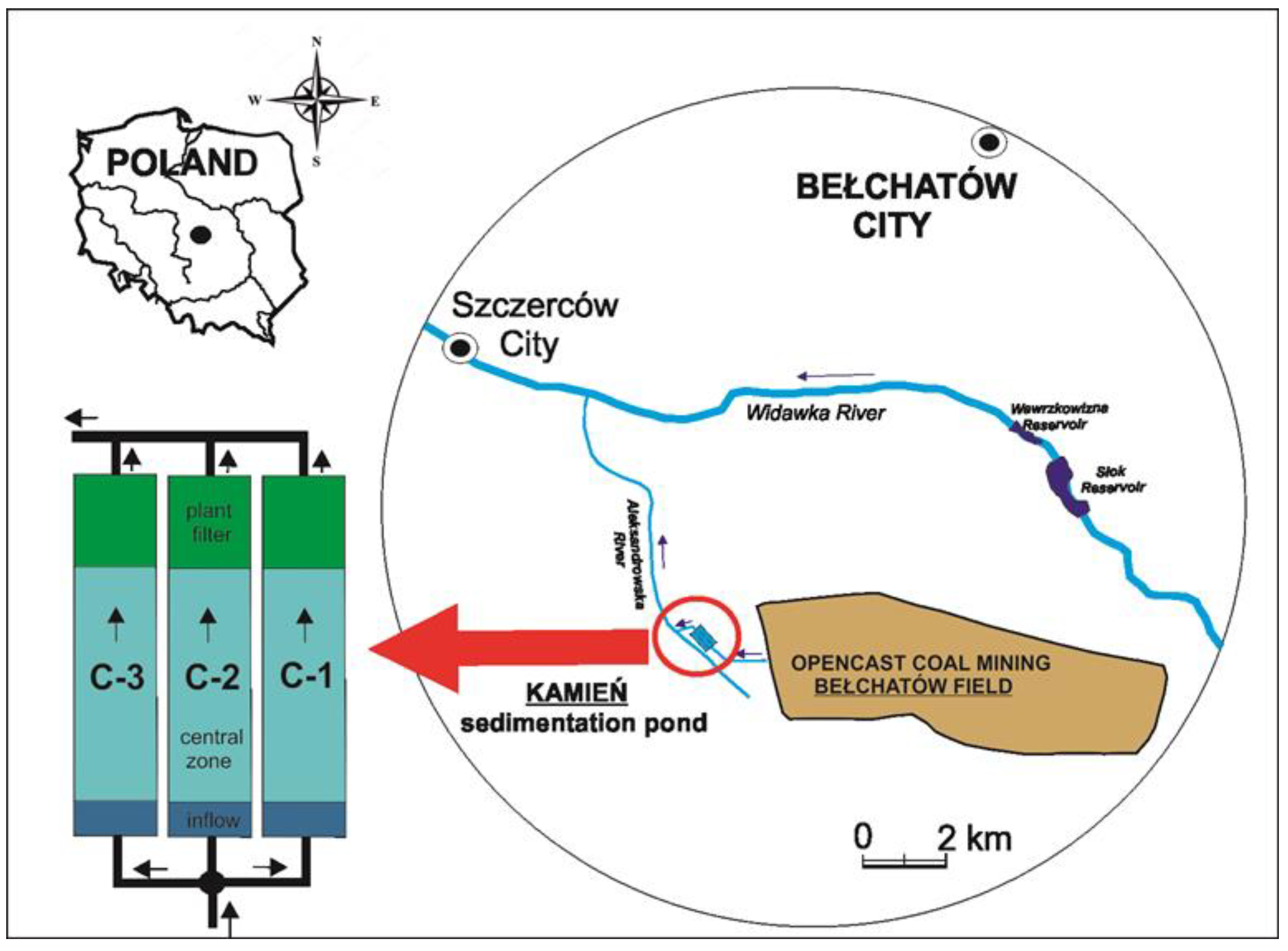
The study was conducted in the reservoirs supplied with water from a dewatering system of the largest opencast brown coal mine, “Bełchatów”, in Poland, in use since 1975. The reservoir complex, named Kamień, is located at the WGS84 point: 51°15′18.9″ N, 19°12′15.4″ E. It is composed of three separate earthen chambers (C-1, C-2, and C-3) situated parallel to each other and separated by dikes ≈ 3.5 m high (Figure 1). The area of each of these ponds is 7.5 ha. The surface drainage system collects water from precipitation and the pit surface. Through pumping stations, this water is directed by pipelines to an open channel that leads to the reservoir complex. A separating well directs a similar volume of water to each of the earthen chambers. With a maximum allowable inflow of 1.8 m3 s−1, the water retention time in each reservoir is approximately 16 h. The complex of the three chambers is used for water treatment by the gravitational sedimentation of colloidal and pseudocolloidal particles suspended in the water. Each chamber consists of three functional zones (Figure 1). The first inflow zone, with an area of approximately 0.1 ha, is used to remove the coarsest fractions of suspended matter. Then, the water flows through an overflowing comb baffle and enters the central zone, which is the main zone of the chamber (area 5.65 ha; maximum depth 2.2 m; capacity 103,000 m3). The process of sedimentation and water clarification is finished in the plant filter zone. This filter (area 0.75 ha; average depth 0.50 m) includes macrophytes such as Phragmites australis (Cav.) Trin. ex Steud., Typha latifolia L., Glyceria maxima (Hartm.) Holmb., Phalaris arundinacea L., Acorus calamus L., and Carex acutiformis L. [6]. There is an outlet behind the filter and the water flows into a collective discharge channel.
2.2. Physicochemical Parameters: Sampling and Analyses
Field surveys were conducted in two biennial cycles, i.e., in 2014/2015 and 2018/2019, including a five-times sampling regime throughout the growing season. Water samples for physicochemical parameters were collected at the main inflow and in the central part of each of the three chambers (C-1, C-2, and C-3) of the Kamień sedimentation pond as representative sampling sites, at the depth of 1 m below the water surface.
Field measurements were performed in situ at each sampling occasion. Water temperature (T), dissolved oxygen (DO) content, and oxygen saturation (%) were measured using the Multi-Parameter Water Quality Sonde YSI 6600 V2, whereas pH and total dissolved solids (TDS) were measured with the digital multimeter HQ30D. In each chamber, the water transparency was measured with a Secchi disk and expressed as the Secchi disk depth (SDD). The ions and trace elements selected for the study were analyzed based on the results of a hydrogeochemical background performed for the area covering the mining activities [17,18], and they were studied at the same sampling sites. Such a range of hydro-analyses coincided with the cyclic monitoring of the mine water quality supervised by the Polish National Hydrogeological Service [19]. The laboratory analyses included total suspended solids (TSS), inorganic suspended solids (ISS), turbidity, total organic carbon (TOC), chlorophyll a (Chl a), total nitrogen (TN), total phosphorous (TP), silicon (Si), calcium (Ca), iron (FeTot), manganese (Mn), phosphate (PO43–), nitrate (NO3–), ammonium nitrogen (NH4+), bicarbonate (HCO3-), sulfate (SO42–), magnesium (Mg2+), and chlorides (Cl−). The hydrochemical analyses were conducted according to the APHA guidelines [20]. Furthermore, the concentrations of selected trace elements, Ag, Al, As, B, Ba, Br, Cd, Cr, Co, Cu, Hg, I, Mo, Ni, Pb, Rb, Se, Sr, Ti, Tl, V, Y, Zn, Zr, were determined with the accuracy of 0.01 μg L−1 according to a methodology based on elementary coupled plasma ionization mass spectrometry (ICP-MS) using an emission spectrometer, Elan ICP-MS (Perkin Elmer).
2.3. Biological Parameters: Sampling and Analyses
The phytoplankton and zooplankton samples were collected five times a year, including the spring, summer, and autumn seasons of each year of the study, from the same sites described for the physicochemical variables. Samples at 1 m depth were taken using the Ruttner sampler (5 L) from the deepest (representative) site. The phytoplankton samples for quantitative analysis were not concentrated, whereas, for taxonomic analysis, they were additionally taken using the plankton net with a 10 μm mesh size. Regarding the zooplankton, the sampled material of 10 L was filtered by a plankton net (a mesh size of 25 μm) for both quantitative and qualitative analyses. The standard Lugol’s solution (I2 in KI) and ethyl alcohol were used to preserve the samples.
The quantitative analysis of phytoplankton, including density (ind. L−1) and biomass (mg L−1), was performed using an inverted microscope according to the standard Utermöhl method [21]. The counted organisms (single cells, colonies, or filaments) were examined at different magnifications: 100×, 200×, and 400×, for large-, medium-, and small-sized taxa, respectively. The qualitative analysis (taxonomic identification) was performed using a light microscope at magnifications of 200×, 400×, and 1000× with oil immersion. The total phytoplankton biomass and the biomass of each species were calculated based on the cell biovolume measurements according to the standard and revised method [22]. Taxonomic identifications were based on the latest references and verified according to currently accepted taxonomic names given in AlgaeBase [23].
The identification and measurements of zooplankton were conducted using the Zeiss AXIO Imager microscope and available references [24,25,26]. The zooplankton density was determined by using a Sedgewick rafter. The density (ind. L−1) and total biomass (mg L−1) of zooplankton were calculated by different methods. The biomass of planktonic crustaceans was determined according to Bottrell et al. [27] and Ruttner-Kolisko [28], whereas the individual body weights of rotifers were based on the standard wet weights according to Ejsmont-Karabin [29].
In each chamber, samples of fish were collected using gillnets, which were set annually in the autumn, i.e., 3 October 2014, 2 October 2015, 5 October 2018, and 4 October 2019, according to the CEN standard protocol [30]. At each time, four gillnets, 30 m long by 1.5 m high, were used in each sedimentation chamber. The gillnets were constructed from 12 panels of 2.5 m long with mesh sizes ranging from 5 to 55 mm. The gillnets were set before sunset and removed after dawn, for a total of 12 h [31]. The fish caught were identified to species level, weighed, and measured with accuracy to one gram and one millimeter, respectively.
The ichthyobiotic indices were calculated according to the CEN standard, including the density (number per unit effort, NPUE) and biomass (weight per unit effort, WPUE) of fish [32]. Monitoring of ichthyofauna did not indicate the occurrence of typically planktivorous fish, i.e., species for which zooplankton is the primary food during its whole life cycle. Thus, it was assumed that only juvenile fish of all species in the first and second years of life have potentially the greatest impact on plankton structure. Studies to date clearly indicate that such fish (total body length <100 mm, individual body weight <25 g) can be caught by gillnets with the smallest mesh [32], Therefore, the density (NPUE, ind. m−2) and biomass (WPUE, g m−2) of planktivorous fish were calculated for fish caught by panels with a mesh size of 5.0, 6.25, 8.0, and 10.0 mm (total 15 m−2 in each gillnet). Fish caught by panels with larger meshes were considered unsuitable for analysis and were excluded from comparisons.
2.4. Biodiversity and Ecological and Trophic Indicators
For the biodiversity assessment, the species richness, Shannon–Weaver diversity index (S-WI; [33]), and Pielou’s evenness index (E; [34]) were calculated from the density of phytoplankton and zooplankton.
The assessment of the ecological potential of each chamber of the Kamień sedimentation pond was based on the phytoplankton index called the Phytoplankton Metric for Polish Lakes (PMPL), and the water quality was classified according to the Polish Regulation [35].
The calculations of PMPL were based on equations adapted from Napiórkowska-Krzebietke et al. [36] and references therein and verified based on data from a similar artificial water body [7]. The assumption criteria included small, shallow, and non-stratified artificial water bodies; a very low ratio of catchment area and lake volume (Schindler’s ratio SR = 0 ≈ SR < 2); very high Ca content (>25 mg dm−3); and a sampling regime of five times a year.
The trophic state, as the trophic level index (TLI) according to Burns et al. [37], was determined for each chamber. The TLI comprises four partial indices based on the total phosphorus (TLITP), total nitrogen (TLITN), Secchi disk depth (TLISDD), and chlorophyll a (TLIChl). The rationale for selecting the TLI was to extend the state evaluation to other seasons, besides summer, which was tested and verified on data from Polish lakes [36]. The final TLI considered the average value obtained from four partial indices. Additionally, the trophic efficiency (TE) was calculated based on the total zooplankton biomass to total phytoplankton biomass ratio. The level of efficiency was classified as follows: class I—0–0.20, class II—0.21–0.40, class III—0.41–0.60, class IV—0.61–0.80, and class V—0.81–1.00, i.e., ranging from the lowest to the highest efficiency [38].
2.5. Statistical Analyses
Abiotic and biotic data were checked for normality with the Shapiro–Wilk test, which confirmed that the data were not normally distributed. Thus, nonparametric analysis of variance (ANOVA) with the Kruskal–Wallis test (to compare more than two independent samples) was the primary tool used to identify the statistical significance of differences between environmental variables among the study periods in the three chambers of the sedimentation pond. The general differences between two biennial periods in the analyzed factors were confirmed with the Mann–Whitney U test (to compare two independent groups). The level of significance was set to a p < 0.05. The relationships between plankton, planktivorous ichthyofauna, and environmental variables were tested with the Spearman’s rank correlation coefficient. These analyses were performed with the Statistica software (ver. 13.3 for Windows, Statsoft, Tulsa, OK, USA).
Non-metric multidimensional scaling (NMDS), as a distance-based ordination technique, based on biotic, abiotic, and indices’ data, was used to separate similar or dissimilar samples taken in the three chambers during the growing seasons in 2014–2015 and 2018–2019. Then, the Bray–Curtis distance measure, two axes, and stress formula type 2 were applied for log-transformed abiotic and biotic parameters. The analysis was conducted using Canoco 5.
3. Results
3.1. Abiotic Parameters and Water Quality
Some key abiotic factors showed significant differences as confirmed by the Kruskal–Wallis test (Table 1). In both periods, statistically significant differences (p < 0.05) were recorded in dissolved oxygen (7.78–8.91 mg L−1 in 2014–2015, and 8.36–9.51 mg L−1 in 2018–2019) and pH (7.51–7.58 in 2014–2015, and 7.61–7.79 in 2018–2019). The concentrations of TP (H = 20.67. p = 0.0043), sulfate (H = 19.53. p = 0.0067), and calcium (H = 17.93. p = 0.0123) were statistically different between the studied seasons (p < 0.05). In 2014–2015, the average concentration of TP in the inflow waters was 0.132 mg L−1 and it was significantly higher than in 2018–2019 (0.089 mg L−1). The same trend was noted in each chamber. The highest average concentration of TP was found in chamber C-1 (0.141 mg L−1) and the lowest in chamber C-3 (0.106 mg L−1) in 2014–2015. Meanwhile, in 2018–2019, the average concentration of TP decreased to 0.074 mg L−1 in chambers C-1 and C-2 and to 0.076 mg L−1 in chamber C-3. In 2014–2015, the average concentration of sulfate ions in the inflow waters was 169.8 mg L−1 and was significantly lower than in 2018–2019 (256.7 mg L−1). A similar upward trend was recorded in each chamber of the Kamień sedimentation pond. In 2014–2015, the highest average concentration of SO4 was found in chamber C-1 (157.0 mg L−1) and the lowest in chamber C-3 (141.3 mg L−1). In the second period, the average concentration of sulfate ions in these chambers was statistically higher and amounted to 238.8 mg L−1 and 236.2 mg L−1, respectively. In 2018–2019, a significant increase in the calcium ion concentration was also recorded. This phenomenon was the most dynamic in chamber C-1, where average values ranged from 107.3 mg L−1 (in 2014–2015) to 153.9 mg L−1 (in 2018–2019). The results indicated an increase in the hardness and salinity of all sedimentation ponds, combined with a decrease in total phosphorus caused by a change in the organic phosphorus fraction. Other indicators, including temperature, SDD, turbidity, TSS, phosphates, total nitrogen, nitrates, ammonium nitrogen, chloride ions, and magnesium ions, despite the variability in the recorded concentrations, in the absence of statistically significant differences, should be considered stable (Table S1).
The trace element concentrations in the Kamień sedimentation pond were characterized by moderate and nonsignificant variability (Table S2). The dominant component was Si, and its average concentration was 15.49 mg L−1, followed by Fe with a concentration ranging within 0.03–2.90 mg L−1, and Mn ranging within 0.05–1.85 mg L−1. Among the elements decisive for the water quality classification, the highest average concentration ranges were for Ba (109.25–113.94 µg L−1), Zn (20.30–32.80 µg L−1), Ti (10.76–12.48 µg L−1), and Al (1.34–4.04 µg L−1), whereas the average concentrations of Ag, As, Cd, and Se did not exceed 0.01 µg L−1. These results allowed us to classify the waters of the Kamień sedimentation pond into the I-II quality class, thus confirming the absence of a toxic threat to hydrobionts from trace elements.
3.2. Biotic Abundance-Based Indicators
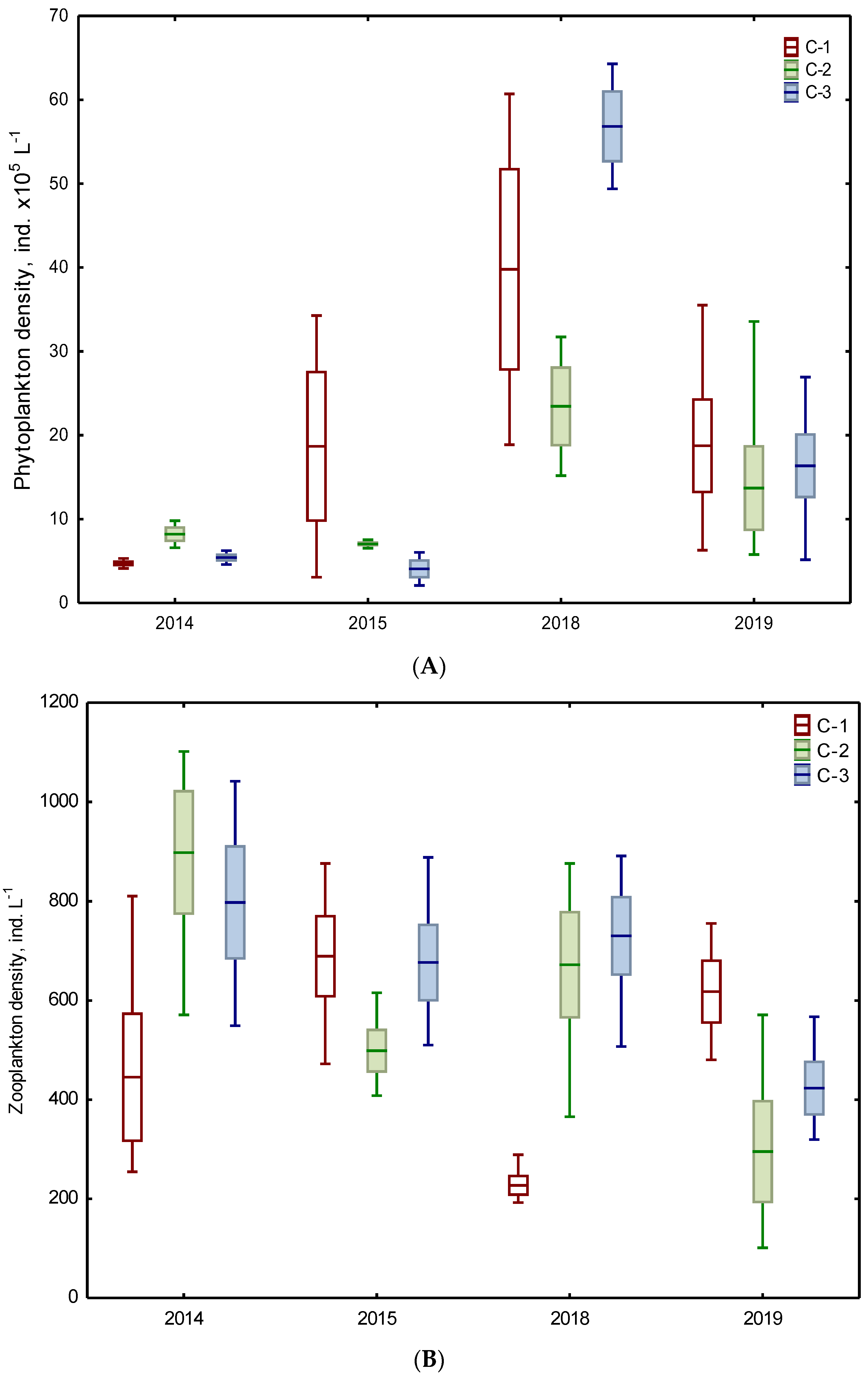
Phytoplankton taxa belonged to eight phyla: Bacillariophyta, Charophyta (planktonic), Chlorophyta, Miozoa, Euglenozoa, Cryptophyta, Ochrophyta, and Cyanobacteria. Phytoplankton density ranged within 3.1–60.7 × 10⁵ ind. L−1, 5.8–33.6 × 10⁵ ind. L−1, and 2.1–64.3 × 10⁵ ind. L−1 in C-1, C-2, and C-3, respectively (Figure 2A). On average, up to 6.7 times lower density was recorded from 2014 to 2015 than between 2018 and 2019. Only the phytoplankton density in chamber C-3 in 2014–2015 was statistically lower than in chamber C-1 in 2018–2019 (Table 2).
The total density of zooplankton ranged generally from ca. 100 ind. L−1 to 1100 ind. L−1 (Figure 2B). On average, the values of density increased from 495 ind. L−1 and 591 ind. L−1 to 657 ind. L−1 in C-1, C-2, and C-3, respectively. However, the higher values were usually noted in the first period of the study (2014–2015).
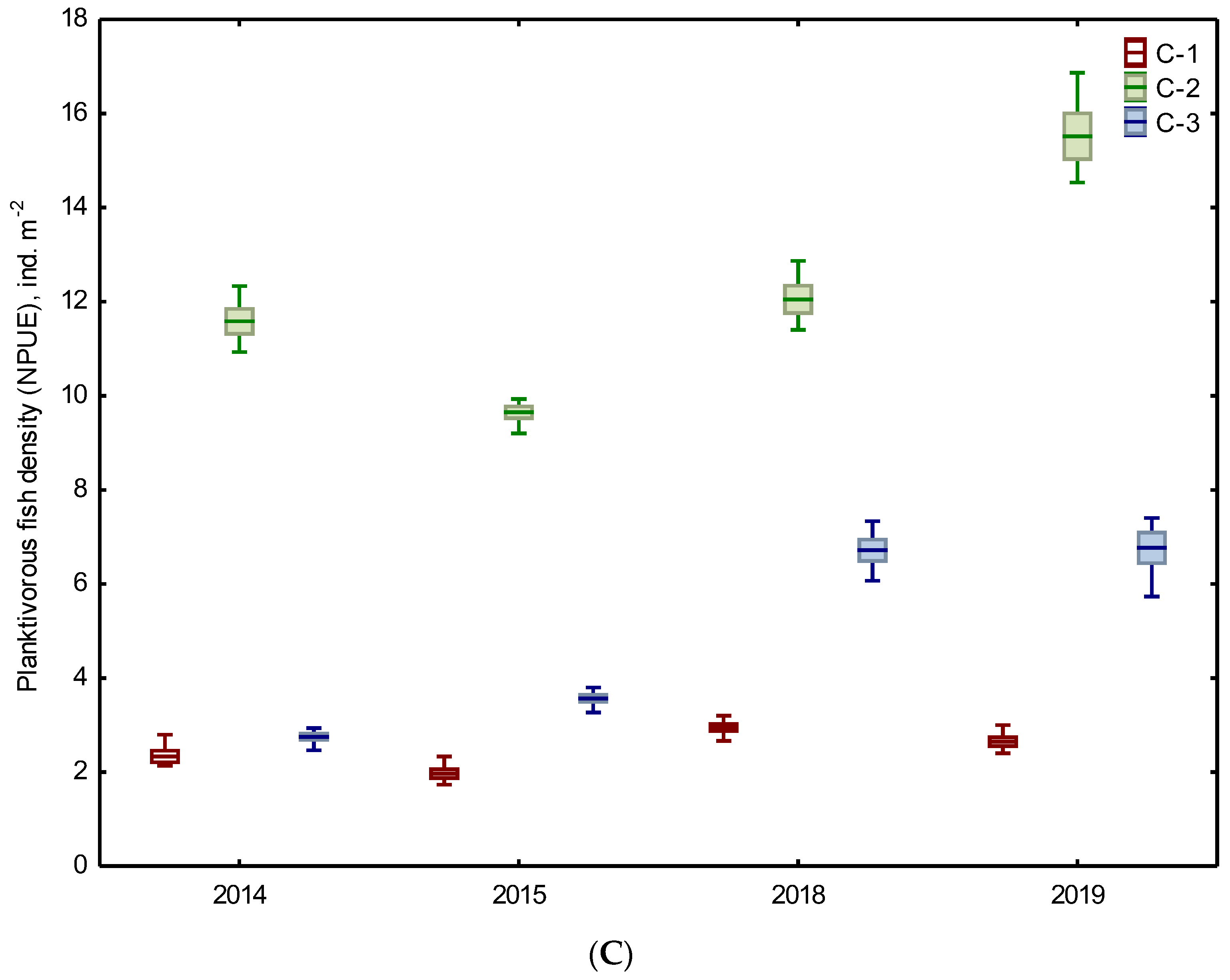
Regarding the planktivorous fish, the average density expressed as NPUE amounted to 2.5 ind. m−2, 12.2 ind. m−2, and 5.0 ind. m−2 in C-1, C-2, and C-3, respectively (Figure 2C). Higher values were recorded from 2018 to 2019 than in 2014–2015 (the Mann–Whitney U test, p = 0.001–0.005). However, in both periods, the fish density in chamber C-1 was the lowest and was statistically different from chamber C-2. In 2018–2019, such differences concerned also the fish density in chamber C-3 (Table 2).
The dominant structure of phytoplankton differed in both the temporal and spatial scales. Based on average values, Cryptophyta had the highest density in 2014, 2018, and 2019 in the selected chambers (Table S3). The most abundant were nanoplanktonic Plagioselmis nannoplanctica (H. Skuja) G. Novarino, I. A. N. Lucas & S. Morrall, and Cryptomonas erosa Ehrenberg. Next, Euglenozoa, including especially Lepocinclis spirogyroides B. Marin & Melkonian, Strombomonas gibberosa (Playfair) Deflandre, Phacus limnophilus (Lemmermann) E. W. Linton & Karnkowska, Phacus longicauda (Ehrenberg) Dujardin, and Phacus tortus (Lemmermann) Skvortsov, dominated or co-dominated the phytoplankton in 2014 and 2015. A high contribution to the total density was noted also for chrysophytes from the genera Chromulina and Dinobryon (dominant in 2018 in C-2 and C-3), large-sized diatoms (2015), and small-sized chlorophytes (2014–2015, and 2019). Among diatoms, these were dominated primarily by Ulnaria acus (Kützing) Aboal, Cymatopleura elliptica (Brébisson) W. Smith, Iconella splendida (Ehrenberg) Ruck & Nakov, and Nitzschia sigmoidea (Nitzsch) W. Smith, which enhanced the total biomass.
Rotifers always prevailed over crustaceans in the zooplankton community (Table S3). The rotifer shares in the total density ranged between 65 and 84% in 2014–2015 and 78 and 92% in 2018–2019, on average, especially due to taxa of the genera Ascomorpha and Polyarthra. The planktivorous fish community constituted ruffle (Gymnocephalus cernua (L.)), bream (Abramis brama (L.)), perch (Perca fluviatilis L.), roach (Rutilus rutilus (L.)), and bleak (Alburnus alburnus (L.)). Roach exclusively dominated in chamber C-2 (72–84%, on average), whereas, in chamber C-3, its share ranged from 31 to 57%, on average. Chamber C-1 was characterized by relatively stable and similar shares of all fish species in the total density. However, a preference for a visibly higher share was seen in the case of roach, especially in 2018–2019.
3.3. Biotic Biomass-Based Indicators
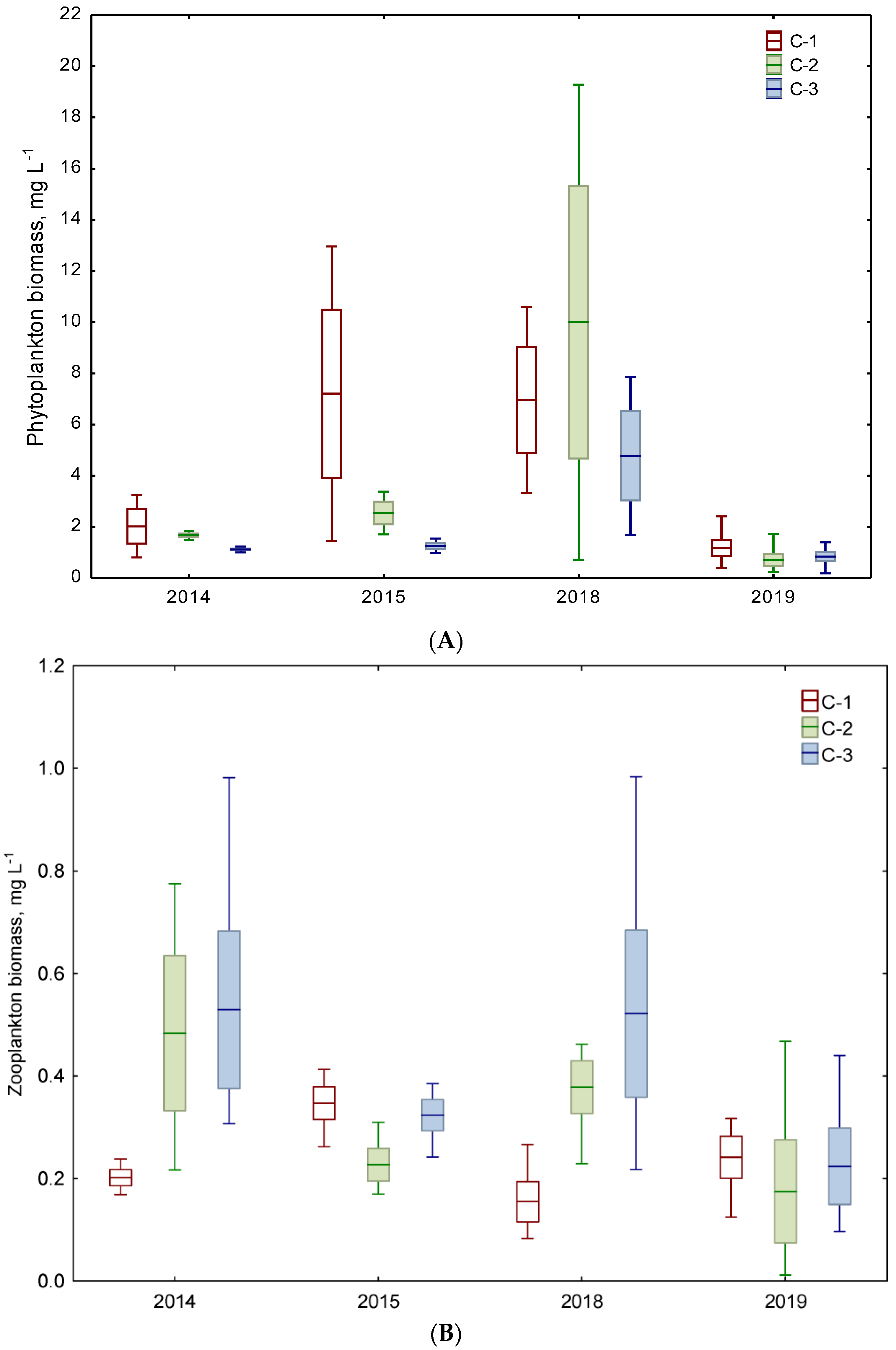
Generally, the average total biomass of phytoplankton in the three chambers ranged between 1.1 and 7.2 mg L−1 and 0.7 and 10.0 mg L−1 in 2014–2015 and 2018–2019, respectively (Figure 3A). However, the differences in the total biomass were not statistically significant in a temporal scale. The only exceptions concerned the significantly different biomasses of Miozoa and Ochrophyta in both periods. The decreasing trend of the total biomass in chambers was as follows: C-1 > C-2 > C-3.
In contrast, a slight increase in zooplankton biomass was noted in the chambers as follows: C-1 < C-2 < C-3. Only a slightly higher average zooplankton biomass was noted in the period of 2014–2015 (0.23–0.51 mg L−1) than in 2018–2019 (0.14–0.49 mg L−1) (Figure 3B).
The lowest average biomass of planktivorous fish (expressed as WPUE) was usually noted in chamber C-1 (8.90–13.20 g m−2), followed by chamber C-3 (15.02–45.30 g m−2), whereas the highest average biomass in chamber C-2 (45.10–74.3 g m−2) showed trends as follows: C-1 < C-3 < C-2 (Figure 3C). Comparing both study periods and each chamber separately, a higher biomass was always recorded in 2018–2019 than in 2014–2015 (the Mann–Whitney U test, p = 0.001–0.004). A significantly different fish biomass was found in chamber C-2 compared to chamber C-1, but not in chamber C-3 (Table 2).
3.4. Biodiversity and Ecological–Trophic Relations
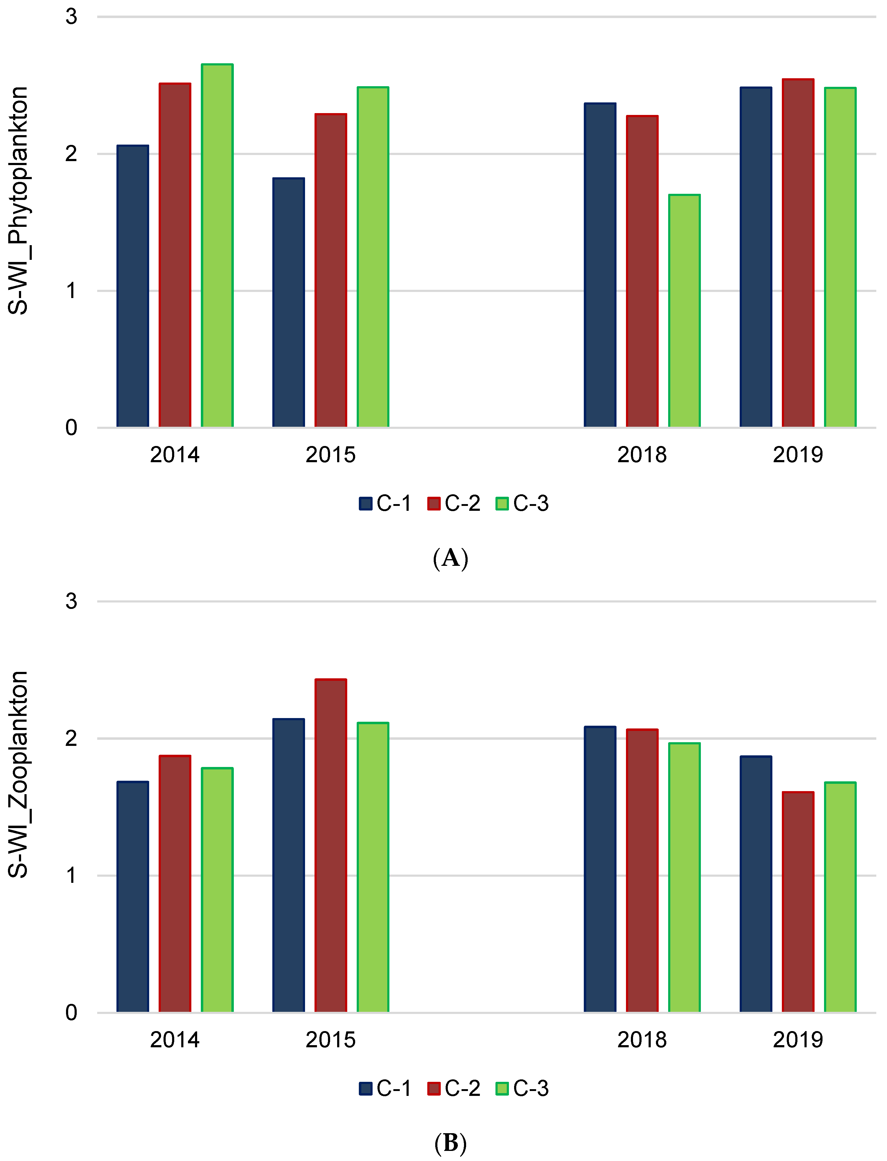
The total phytoplankton species richness of 150 taxa at the level of species, variety, and form was recorded for all chambers, including 107, 118, and 98 taxa in C-1, C-2, and C-3, respectively. Regarding the phytoplankton diversity, the values of the Shannon–Weaver index (S-WI) ranged from 1.6 to 2.6, on average (Figure 4A), and slightly differed spatially (chambers) and temporally (years of study). The evenness ranged, then, from 0.476 to 0.802. The highest biodiversity was recorded in C-3 in 2014, whereas the lowest was found in 2018.
For zooplankton, the total species richness was estimated at 42 for all chambers. The values of S-WI ranged from 1.6 to 2.4, with a minimum in chamber C-2 in 2019 and a maximum in chamber C-2 in 2015 (Figure 4B). Furthermore, the evenness was in the range of 0.638–0.825.
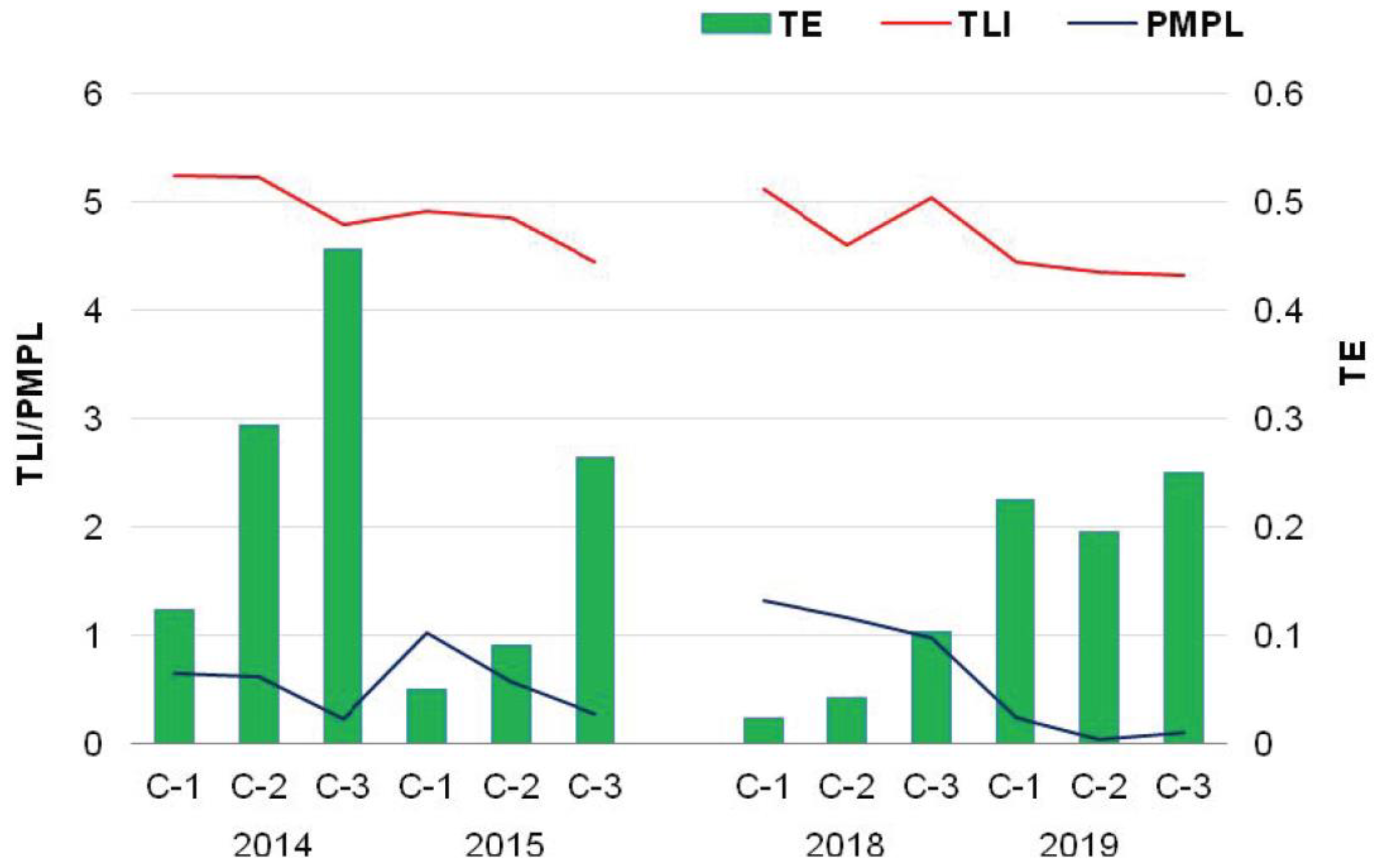
The trophic conditions were analyzed based on the average TLI values obtained from partial indices TLI-TP, TLI-TN, TLI-SDD, and TLI-Chl. The highest values of TLI were recorded in chamber C-1 (4.5–5.3), followed by chamber C-2 (4.4–5.2) and chamber C-3 (4.3–5.1), indicating a general eutrophic level with some exceptions in 2014 and 2018 (Table 3). Higher variability was recorded within partial indices. The highest values were seen for TLI-TP, especially in 2014 (6.6–6.8), and the lowest for TLI-Chl, especially in 2019 (3.1–3.5). The general relations between partial indices were as follows: TLI-TP > TLI-SDD > TLI-TN > TLI-Chl (6.0, 5.5, 4.0, 3.7 on average, respectively).
Similar to the trophic conditions, the values of the final multimetric PMPL were characterized by relatively low variation, i.e., from 0.03 to 1.32, indicating the first and the second class, i.e., maximum or good ecological potential (Table 4). The values of partial metrics changed within wider ranges, especially MTB (0.02–2.84), whereas MCB was stable (0.10). Generally, the best water quality class (maximum ecological potential) was recorded in 2014 and 2019 and the worst water quality in 2018 (good potential in chambers C-1 and C-2).
The zooplankton and phytoplankton dependence expressed as trophic efficiency ranged from 0.02 to 0.46 in all chambers (Figure 5). However, the differences in TE values between chambers were as follows: C-1 < C-2 < C-3, with the average values of 0.11, 0.16, and 0.27 indicating classes I and II. An exception was noted in 2019, when the TE values were very similar in all chambers. This phenomenon suggests that the ecological conditions were intermediate in 2019. Similar trends were also found for the phytoplankton and zooplankton density and ecological and trophic conditions as well.
3.5. Biotic–Abiotic Relationship
Generally, the biotic–abiotic relationships were tested with Spearman’s correlations (Table 5). These results confirmed the strong relations between the total phytoplankton biomass and most of the analyzed parameters. A negative correlation was found with SDD (correlation coefficients R = −0.575). In other cases, there were positive correlations, i.e., between TB_Phyto and TSS, turbidity and color (R ranges 0.520–0.594), TP and Porg (R = 0.452 and R = 0.447, respectively), and nitrogen compounds (TN − R = 0.483, NH43− − R = 0.507, NO3– − R = 0.624). Similarly, positive relations were observed for the phytoplankton density and pH (R = 0.706), TSS (R = 0.467), and turbidity (R = 0.417). Fish biomass (WPUE) and density (NPUE) were negatively correlated with TOC (R = −0.496 and −0.504, respectively).
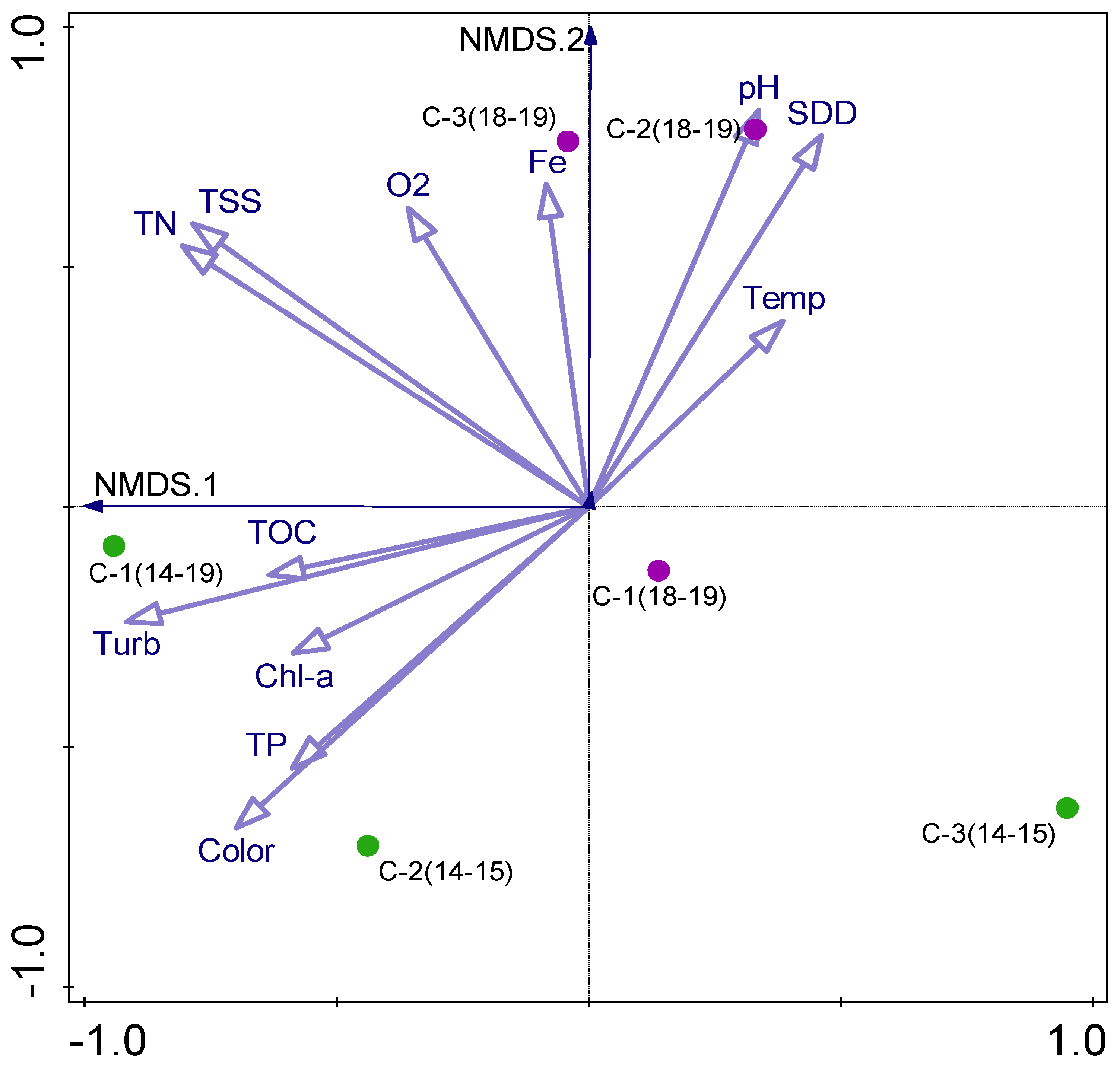
Finally, all multivariate data sets, including key abiotic and biotic factors, and ecological versus trophic interactions in two biennial periods were checked in a reduced ordination space with NMDS. The NMDS analysis, based on physicochemical parameters with a stress value of 0.00040735, allowed us to distinguish two separate groups of samples (Figure 6). The first group comprised samples taken in 2014–2015 from chambers C-1 and C-2, with higher values of the following variables: TOC, Turb, Chl-a, and TP. The second group, with samples taken in 2018–2019 from chambers C-2 and C-3, was separated due to higher values of pH, SDD, Temp, Fe, O2, TSS, and TN. The samples from chambers C-3 (2014–2015) and C-1 (2018–2019) were different from the others, showing lower values mainly of TN, TSS, O2, and Fe.
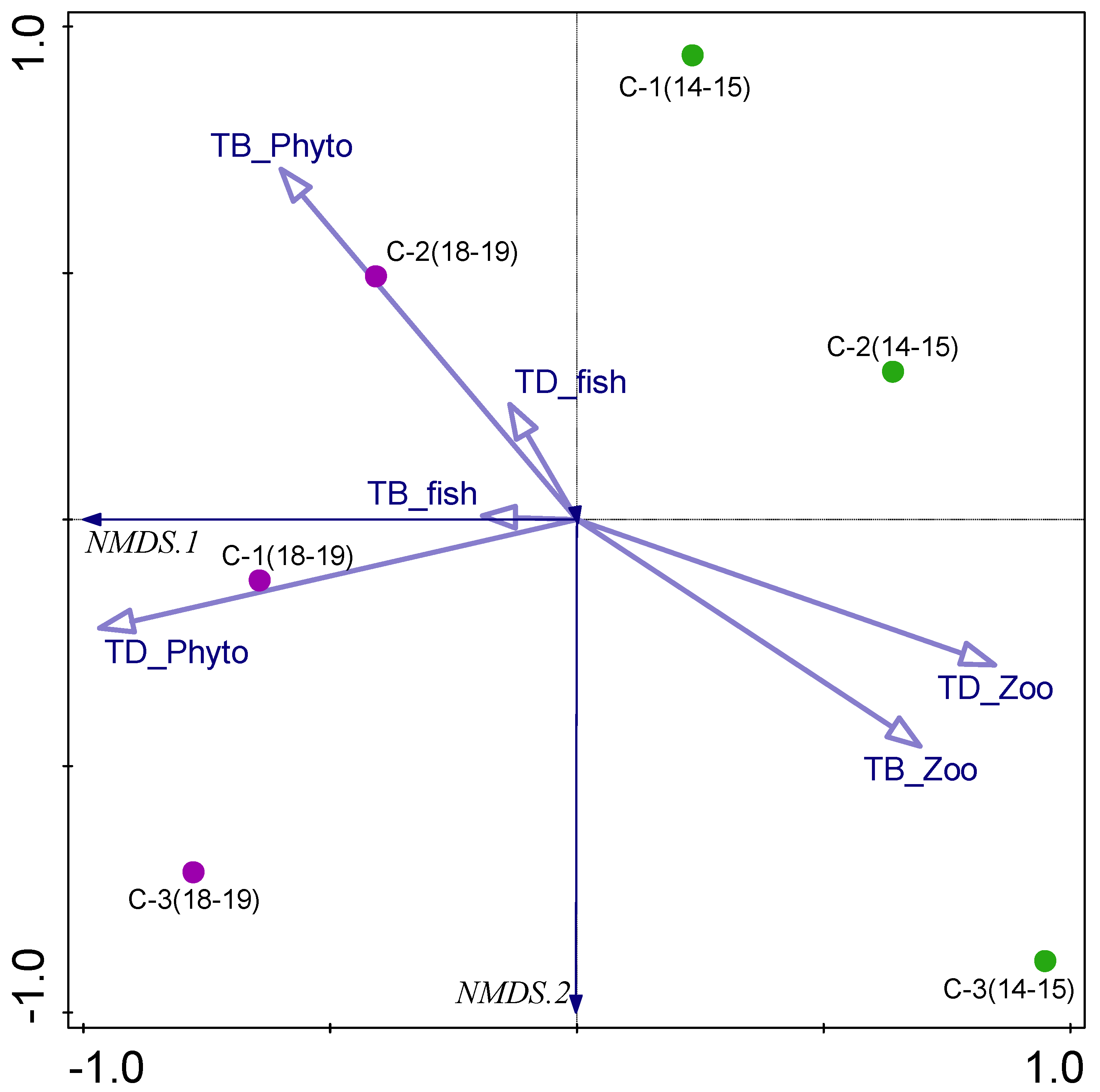
An NMDS analysis based on biological parameters with the stress value of 0.00018004 was able to separate samples taken in 2018–2019 from chambers C-1 and C-3, mostly due to phytoplankton density, and samples from chamber C-2 due to phytoplankton biomass (Figure 7). The zooplankton density and biomass impacted the separation of the samples from chamber C-3 taken in 2014–2015. The samples from chambers C-1 (2014–2015) and C-2 (2014–2015) were different from the others.
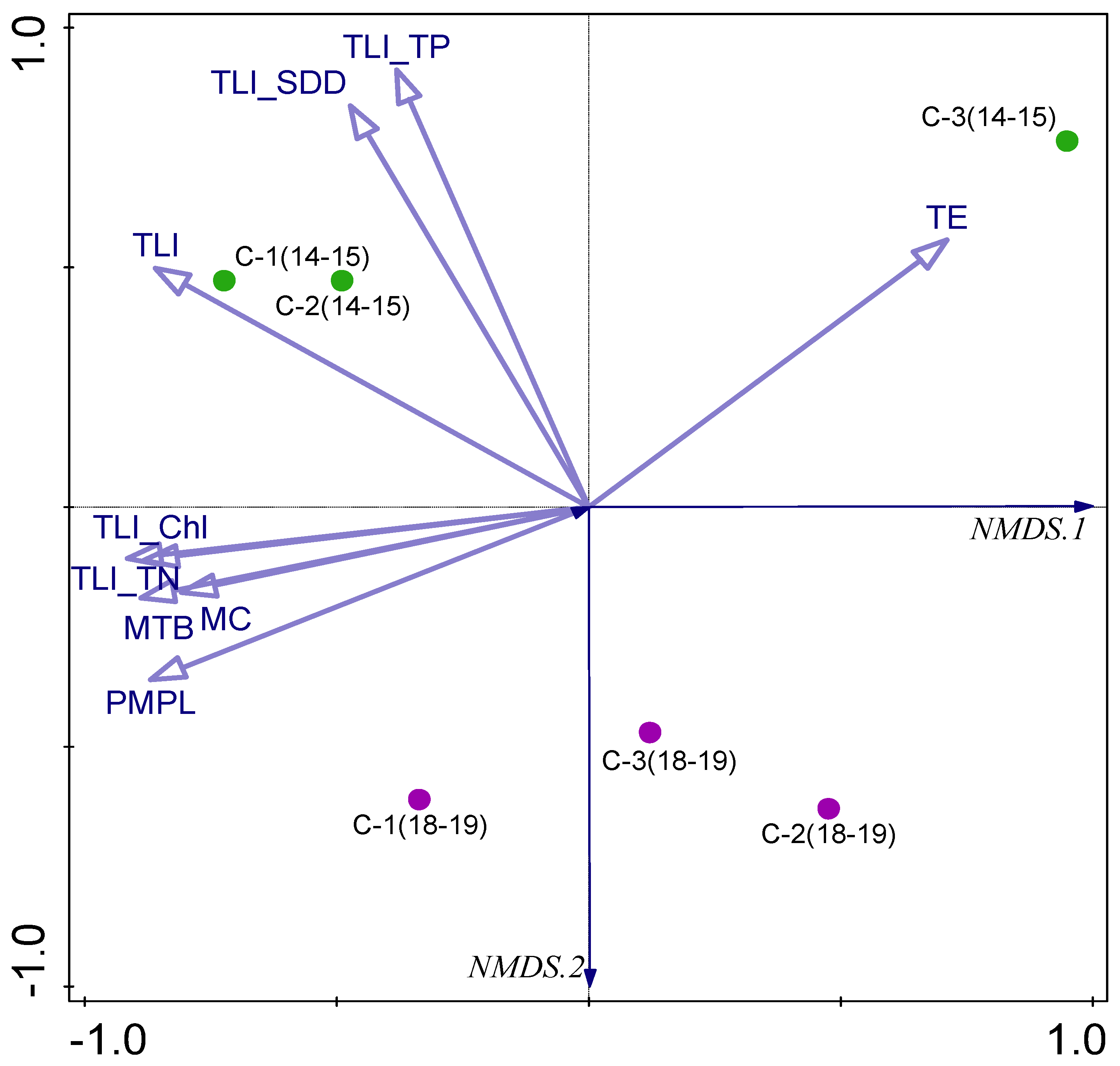
The NMDS analysis based on ecological and trophic indices with the stress value of 0.00028063 also confirmed the above-mentioned differences and showed the general separation of samples taken in 2014–2015 from those taken in 2018–2019 (Figure 8). The TLI and some partial TLI indices impacted the separation of samples from chambers C-1 (2014–2015) and C-2 (2014–2015), other TLI indices and PMPL and partial metrices were mostly connected with chamber C-1 (2018–2019), and TE determined the distinction of samples from chamber C-3 (2014–2015).
4. Discussion
The studied water body (the Kamień sedimentation pond) was supplied with water from an opencast mine characterized by a relatively pristine catchment area. The water chemistry and the dynamics of changes in chemical composition were consistent with the hydrogeochemical background [17,18]. This confirmed that the impact of the catchment area on this pond was not significant. The geochemistry of the rocks in the area of the drained open-pit mine indicates their bicarbonate concentration and organogenic structure [39]. Therefore, the sediment ponds are supplied with weakly alkaline calcium bicarbonate water. The relatively high concentrations of calcium and bicarbonate are beneficial because they stabilize the alkaline water. Phosphate’s affinity for calcium, iron, and manganese ions under stable aerobic conditions and in alkaline water limits primary production. Such relations and increases in the concentrations of calcium and sulfate ions were noted by identifying the hydrochemical properties of the mine water [7,8]. The development of plankton may be limited by the large amount of suspended solids, including mechanical aspects of creating aggregates and causing its sinking, as well as limiting access to light [40,41]. Similar observations were demonstrated in studies of other reservoirs supplied with mine water [8]. Furthermore, the flocculation process involving both the phytoplankton and zooplankton is one of the key factors in suspension sedimentation [42,43].
The current study assessed the phytoplankton and zooplankton assemblages under planktivorous fish pressure, as well as specific environmental conditions. Generally, phytoplankton growth was much higher than zooplankton growth, which was confirmed by the biomass-based trophic efficiency at a low level [38]. However, relatively high biodiversity for both planktonic organisms was recorded and confirmed by the species richness (150 and 42 for phytoplankton and zooplankton, respectively), Shannon–Weaver index (up to 2.6 and 2.4, respectively), and evenness (up to 0.802 and 0.825, respectively), similarly to the biodiversity noted in small and shallow lakes [38]. Phytoplankton were dominated by cryptophytes of the genus Cryptomonas, which are considered to be either phototrophic or mixotrophic and represent codon Y, referring to a wide range of habitats and reflecting their ability to live in almost all lentic ecosystems when the grazing pressure is low [44]. However, the second most dominant group was euglenoids belonging to codon W1, which is typical of ponds, even temporary, rich in organic matter from husbandry or sewages, suggesting a more fertile environment. These two groups were not recorded as dominant groups in the other ponds fed with water of the same origin, and, on the contrary, phytoplankton were dominated primarily by diatoms [7,8]. Large-sized diatoms, which are important for the flocculation process of mineral particles in sedimentation ponds [45], dominated only in 2015 (Kamień sedimentation pond).
The trophic levels were similar in all chambers, indicating eutrophy in general (TLI ranging within 4–5 according to Burns et al. [37]), although they tended to slightly decrease in the order C-1 > C-2 > C-3, with higher values in 2014–2015 than in 2018–2019. A similar trend was noted for the phytoplankton biomass, in contrast to the zooplankton biomass. This is in line with the bottom-up (food availability) and top-down (zooplankton grazing) controls of primary production [46]. The trend in the planktivorous fish biomass was different from the abovementioned one. The top-down and bottom-up effects on plankton–fish dynamics were discussed by Pal and Chatterjee [47,48], who confirmed that fish predation determines the abundance of herbivorous zooplankton, which, in turn, regulates phytoplankton biomass. However, it is also dependent on the growing season, especially due to the widely varied predatory zooplankton pressure on herbivorous zooplankton [49]. Thus, any changes in the abundance of planktivorous fish can directly affect both phytoplankton and zooplankton, but the role of omnivorous or predatory fish is also known. At high fish densities, the zooplankton biomass is controlled by fish predation, and the phytoplankton biomass is limited by light or nutrients [47]. In contrast, at low fish densities, zooplankton growth is limited by food resources, and phytoplankton growth is controlled by zooplankton grazing. Generally, planktivorous fish can be identified as an important factor in maintaining at least a good ecological status in aquatic ecosystems. The positive correlations between phytoplankton and TSS, turbidity, and color compounds indicated its influence on the water quality, connected with the shading conditions in water, and such relationships were opposite to those described for other mine waters [7,8]. Such close relations were not observed either for zooplankton or planktivorous fish, and their role in the flocculation process is not well known yet.
Eutrophication is directly related to an increase in the amount of organic carbon in the aquatic ecosystem and, thus, contributes to the increased rate of deoxygenation in water bodies [12]. Such a process is usually accompanied by relatively high biomasses of phytoplankton and zooplanktivorous fish. In the case of sedimentation ponds, the fish biomass was relatively low, and therefore its impact on zooplankton resources was not significant. However, results from some long-term biomanipulation experiments show that a moderate level of planktivorous fish biomass can optimize and stabilize the water quality indices by suppressing invertebrate predation while maintaining an effective biomass of cladocerans [50]. A prey selection strategy to secure the nutritional needs of juvenile fish has been identified by Reissig et al. [51]. It was confirmed that fish are effective nutrient transporters in the lake and can potentially influence primary production [52]. Furthermore, the direct nutrient transport by animals can be significant when their biomass is high enough [53]. In shallow water habitats, where phytoplankton and submerged plants coexist, the constraints on primary production through the C-N-P relationship and the mechanisms that promote organic carbon formation are poorly understood. At the same time, phytoplankton and submerged plants have been found to contribute similar amounts of TOC to water [54]. If fish accumulate nutrients from zooplankton in their bodies, they may be treated as nitrogen, phosphorus, and carbon sinks in the water column zone [55]. According to Kazama et al. [56], the herbivores to primary producers’ biomass relations reflect the structure of the aquatic community. Furthermore, multiple factors affect these relations, especially the production rate, defense traits, nutrients, and predation.
The PMPL-based assessment indicated the maximum or good ecological potential of the sedimentation pond, i.e., it met the WFD’s required goal to achieve at least good potential of the water body [4]. An analogous situation was confirmed for the trace elements, which are decisive for water quality classification (class I–II, at least good ecological potential). The statistically significant differences in fish density and fish biomass in each chamber between the two biennial periods (2014–2015 and 2018–2019) did not result in any significant variation in zooplankton density or biomass. Ichthyobiotic indices of planktivorous fish showed some variability and maintained relative proportions between chambers in the order C-1 < C-3 < C-2, which also did not correspond with zooplankton.
The sedimentation ponds with recreational and angling functions, including also the Kamień sedimentation pond, are periodically stocked mainly with older non-predatory fish, e.g., carp, tench, and ide, which do not feed on zooplankton [57]. Stocking with predatory fish (mainly pike and pikeperch) was similarly low in each chamber, and also it did not include planktivorous species, which could be caught by anglers. It should be assumed that the planktivorous fish density and biomass are mostly dependent on the effectiveness of natural spawning and food conditions and, furthermore, are subjected to changes as a result of different intensities of predation pressure, the efficiency of natural reproduction, and economic procedures (exploitation and stocking). The mechanisms of the direct and indirect effects of these factors have been investigated with biomanipulation treatments [58]. Potentially greater pressure of predatory fish on zooplanktivorous species may have occurred in chamber C-1, which is an angler-operated chamber following the “Catch and Release” model [57]. Furthermore, it was found that in chambers C-2 and C-3, the planktivorous fish assemblages were dominated by roach, the most common species in European waters. According to Maszczyk et al. [59], roach eat less while feeding in a group, both due to food-grabbing tactics and non-aggressive competition for a space. Nevertheless, it should be considered that ichthyobiotic indicators potentially shaped the ecological and trophic conditions of the studied sediment ponds to the least extent.
Despite some spatial and temporal variations in phytoplankton, zooplankton, and planktivorous fish among all chambers of the Kamień sedimentation pond, it was also possible to note that the last year of study (2019) suggested the stabilized conditions of such ecosystems with relatively high biodiversity, a lower eutrophic level, and maximum ecological potential. A similar phenomenon was verified for the other pond supplied with mine water, where the final water stabilization resulted in the abundant growth of charophyte Nitella mucronate and at least good ecological potential [8].
5. Conclusions
On a temporal scale, some significant variations in abiotic and biotic factors were recorded, especially for pH, DO, PO43−, TP, NH4+, NO3−, and TDS, and for fish density and biomass and phytoplankton density. The assessment of the trophic conditions confirmed the eutrophic level in all chambers, whereas the water quality assessment indicated maximum or good ecological potential, i.e., meeting the WFD’s required goal to achieve at least good water status or potential. The analyses of biological factors proved that phytoplankton were quite abundant, whereas zooplankton and planktivorous fish were limited. Thus, the mechanisms of the top-down and bottom-up effects were revealed in all chambers. Spatial differentiations were not so obvious. However, the most sustainable conditions of such ecosystems concerning relatively high biodiversity, phytoplankton, and zooplankton abundances, biomass-based trophic efficiency, and ecological and trophic conditions were found especially in 2019. The present studies indicated that the biomass and density of planktivorous fish in the sedimentation pond were negatively correlated with the TOC concentration because TOC may not be an adequate indicator to interpret the ecological conditions of sedimentation ponds.
The current studies confirmed that phenomena characteristic of natural shallow water bodies occur in artificial reservoirs fed with water from mine drainage and serve as sedimentation ponds. Furthermore, there is the possibility to stabilize the favorable ecological conditions, which, in turn, are necessary to obtain and maintain the full usable functionality of sedimentation ponds and waters from the surface drainage system of an opencast mine. This all proves the importance of an understanding of ecosystem functioning in newly created water bodies related to new knowledge on aquatic organisms, biodiversity, and ecological–trophic relations. It is especially important in urbanized and post-industrial areas for their rational management and optimal use with respect to their ecological functioning and the fulfilment of social needs.
Supplementary Materials
The following supporting information can be downloaded at: https://www.mdpi.com/article/10.3390/w15193328/s1, Table S1: Physicochemical parameters of water in the Kamień sedimentation pond (inflow and chambers: C-1, C-2, C-3) during the growing seasons in 2014–2015 and 2018–2019 (mean, ±SD); Table S2: Average content of trace elements in the Kamień sedimentation pond during the growing seasons in 2014–2015 and 2018–2019 with classification of water quality [35]; Table S3: An average structure of phytoplankton, zooplankton, and planktivorous fish (% of the total density) in three chambers (C-1, C-2, C-3) of the Kamień sedimentation pond during the growing seasons in 2014–2015 and 2018–2019.
Author Contributions
Conceptualization, A.N.-K. and A.R.S.; methodology, A.N.-K. and A.R.S.; validation, A.N.-K. and A.R.S.; formal analysis, A.N.-K.; investigation, A.N.-K., A.R.S. and A.K.; resources, A.N.-K. and A.R.S.; data curation, A.N.-K. and A.R.S.; writing—original draft preparation, A.N.-K. and A.R.S.; writing—review and editing, A.N.-K., A.R.S. and A.K.; visualization, A.N.-K. and A.R.S. All authors have read and agreed to the published version of the manuscript.
Funding
This study was partly conducted within statutory research topics Z-014 and the publication cost was co-financed by the scholarship fund of the National Inland Fisheries Institute in Olsztyn, Poland. The project was financially supported by the Minister of Education and Science under the program entitled “Regional Initiative of Excellence” for the years 2019–2023, Project No. 010/RID/2018/19, amount of funding 12,000,000 PLN.
Institutional Review Board Statement
We confirm that all data collection and analyses were carried out in accordance with relevant guidelines and regulations including CEN standard protocols. We confirm that all experimental protocols were approved by the Research Ethics Committee of the University of Warmia and Mazury in Olsztyn and it was complied with local and national regulations (Decision No. 74/2022). Samples of fish obtained by gillnetting were taken according to the official CEN standard protocol (CEN, 2005. Water Quality—Sampling of Fish with Multimesh Gillnets. European Committee for Standardization, EN 14757, Brussels. https://doi.org/10.3403/30100308). Fish samples were taken in an artificial water body located in the area of an active mining site. In cooperation with the PGE Mining and Conventional Power Generation SA Branch KWB Bełchatów, for the collection of all samples, all relevant permits and permissions were obtained.
Data Availability Statement
All data generated and analyzed during this study are included in this article and in its Supplementary Materials.
Conflicts of Interest
The authors declare no conflict of interest.
References
- Schultze, M.; Pokrandt, K.-H.; Hille, W. Pit lakes of the Central German lignite mining district: Creation, morphometry and water quality aspects. Limnologica 2010, 40, 148–155. [Google Scholar] [CrossRef]
- Blanchette, M.L.; Lund, M.A. Pit lakes are a global legacy of mining: An integrated approach to achieving sustainable ecosystems and value for communities. Curr. Opin. Sustain. 2016, 23, 28–34. [Google Scholar] [CrossRef]
- Liu, Q.; Sun, Y.; Xu, Z.; Jiang, S.; Zhang, P.; Yang, B. Assessment of Abandoned Coal Mines as Urban Reservoirs. Mine Water Environ. 2019, 38, 215–225. [Google Scholar] [CrossRef]
- The European Parliament. Water Framework Directive (WFD) 2000/60/EC: Directive 2000/60/EC of the European Parliament and of the Council of 23 October 2000 Establishing a Framework for Community Action in the Field of Water Policy; The European Parliament: Strasbourg, France, 2000. [Google Scholar]
- Jawecki, B.; Dąbek, P.B.; Pawęska, K.; Wei, X. Estimating Water Retention in Post-mining Excavations Using LiDAR ALS Data for the Strzelin Quarry, in Lower Silesia. Mine Water Environ. 2018, 37, 744–753. [Google Scholar] [CrossRef]
- Stachowski, P.; Kraczkowska, K.; Liberacki, D.; Oliskiewicz-Krzywicka, A. Water Reservoirs as an Element of Shaping Water Resources of Post-Mining Areas. J. Ecol. Eng. 2018, 19, 217–225. [Google Scholar] [CrossRef]
- Skrzypczak, A.R.; Napiórkowska-Krzebietke, A. Identification of hydrochemical and hydrobiological properties of mine waters for use in aquaculture. Aquac. Rep. 2020, 18, 100460. [Google Scholar] [CrossRef]
- Napiórkowska-Krzebietke, A.; Skrzypczak, A.R. A new charophyte habitat with a stabilized good ecological potential of mine water. Sci. Rep. 2021, 11, 14564. [Google Scholar] [CrossRef]
- European Commission. Communication from the Commission to the European Parliament, the Council, the European Economic and Social Committee and the Committee of the Regions: EU Biodiversity Strategy for 2030. Bringing Nature Back into Our Lives; COM/2020/380 Final; European Commission: Brussels, Belgium, 2020. [Google Scholar]
- Claeys, G.; Tagliapietra, S.; Zachmann, G. How to Make the European Green Deal Work; Bruegel, JSTOR: New York, NY, USA, 2019; pp. 1–21. Available online: http://www.jstor.org/stable/resrep28626 (accessed on 1 December 2022).
- Hermoso, V.; Carvalho, S.B.; Giakoumi, S.; Goldsborough, D.; Katsanevakis, S.; Leontiou, S.; Markantonatou, V.; Rumes, B.; Vogiatzakis, I.N.; Yates, K.L. The EU Biodiversity Strategy for 2030: Opportunities and challenges on the path towards biodiversity recovery. Environ. Sci. Policy 2022, 127, 263–271. [Google Scholar] [CrossRef]
- Anderson, N.J.; Bennion, H.; Lotter, A.F. Lake eutrophication and its implications for organic carbon sequestration in Europe. Glob. Chang. Biol. 2014, 20, 2741–2751. [Google Scholar] [CrossRef]
- Vishnu, D.; Dhandapani, B.; Kumar, K.S.; Balaji, G.; Mahadevan, S. Chapter 8—Removal of heavy metals from mine waters by natural zeolites. In New Trends in Removal of Heavy Metals from Industrial Wastewater; Shah, M.P., Couto, S.R., Kumar, V., Eds.; Elsevier: Amsterdam, The Netherlands, 2021; pp. 161–175. [Google Scholar] [CrossRef]
- Mantero, J.; Thomas, R.; Holm, E.; Rääf, C.; Vioque, I.; Ruiz-Canovas, C.; García-Tenorio, R.; Forssell-Aronsson, E.; Isaksson, M. Pit lakes from Southern Sweden: Natural radioactivity and elementary characterization. Sci. Rep. 2020, 10, 13712. [Google Scholar] [CrossRef]
- Dolný, A.; Harabiš, F. Underground mining can contribute to freshwater biodiversity conservation: Allogenic succession forms suitable habitats for dragonfies. Biol. Conserv. 2012, 145, 109–117. [Google Scholar] [CrossRef]
- St-Gelais, N.F.; Jokela, A.; Beisner, B.E. Limited functional responses of plankton food webs in northern lakes following diamond mining. Can. J. Fish. Aquat. Sci. 2017, 75, 26–35. [Google Scholar] [CrossRef]
- Zdechlik, R.; Kania, J. Hydrogeochemical background and distribution of indicator ion concentrations in the region of the Bełchatów lignite deposit. Contemp. Probl. Hydrogeol. 2003, 11, 327–334. (In Polish) [Google Scholar]
- Pękala, A. The Mineral Character and Geomechanical Properties of the Transitional Rocks from the Mesozoic-Neogene Contact Zone in the Bełchatów Lignite Deposit. J. Sust. 2014, 13, 10–14. [Google Scholar] [CrossRef]
- Gogacz, M. The analysis of the quality of waters from mining plant open pit brown coal „Belchatow” joint—Stock company off the surface waterways. In Proceedings of the Mining Workshops from the Cycle “Natural Hazards in Mining”: Symposium Materials: Occasional Session: Problems of Natural Hazards in Brown Coal Mining, Bełchatów, Poland, 2–4 June 2004; Pilecka, E., Ed.; IGSMiE PAN, Cracow, Series: Symposia and Conferences. Volume 62, pp. 139–151. [Google Scholar]
- APHA. Standard Methods for the Examination of Water and Wastewater, 20th ed.; American Public Health Association: Washington, DC, USA, 1999; Available online: https://www.mwa.co.th/download/file_upload/SMWW_1000-3000.pdf (accessed on 4 January 2019).
- Utermöhl, H. Guidance on the quantitative analysis of phytoplankton—Methods. Mitteilungen Int. Ver. Für Theor. Angew. Limnol. 1958, 9, 1–38. (In German) [Google Scholar]
- Napiórkowska-Krzebietke, A.; Kobos, J. Assessment of the cell biovolume of phytoplankton widespread in coastal and inland water bodies. Water Res. 2016, 104, 532–546. [Google Scholar] [CrossRef]
- Guiry, M.D.; Guiry, G.M. AlgaeBase. In World-Wide Electronic Publication; National University of Ireland: Galway, Ireland, 2013; Available online: http://www.algaebase.org (accessed on 12 July 2022).
- Flössner, D. Krebstiere, Crustacea. In Kiemen- und Blattfüsser, Branchiopoda, Fischläuse, Branchiura; VEB Gustav Fischer Verlag: Jena, Germany, 1972. [Google Scholar]
- Ejsmont-Karabin, J.; Radwan, S.; Bielańska-Grajner, I. Rotifers. Monogononta—Atlas of species. In Polish Freshwater Fauna; University of Łódź: Łódź, Poland, 2004. (In Polish) [Google Scholar]
- Błędzki, L.A.; Rybak, J.I. Freshwater crustacean zooplankton of Europe: Cladocera & Copepoda (Calanoida, Cyclopoida). In Key to Species Identification with Notes on Ecology, Distribution, Methods and Introduction to Data Analysis; Springer International Publishing: Cham, Switzerland, 2016. [Google Scholar]
- Bottrell, H.H.; Duncan, A.; Gliwicz, Z.M.; Grygierek, E.; Herzig, A.; Hillbricht-Ilkowska, A.; Kurasawa, H.; Larsson, P.; Weglenska, T. A review of some problems in zooplankton production studies. Norw. J. Zool. 1976, 24, 419–456. [Google Scholar]
- Ruttner-Kolisko, A. Suggestions for biomass calculation of planktonic rotifers. Arch. Hydrobiol. Beih. Ergebn. Limnol. 1977, 8, 71–76. [Google Scholar]
- Ejsmont-Karabin, J. Empirical equations for biomass calculation of planktonic rotifers. Pol. Arch. Hydr. 1998, 45, 513–522. [Google Scholar]
- BS EN 14757:2005; Water Quality—Sampling of Fish with Multimesh Gillnets. European Committee for Standardization: Brussels, Belgium, 2005. [CrossRef]
- Deceliere-Vergẻs, C.; Argillier, C.; Lanoiselée, C.; De Bortoli, J.; Guillard, J. Stability and precision of the fish metrics obtained using CEN multi-mesh gillnets in natural and artificial lakes in France. Fish. Res. 2009, 99, 17–25. [Google Scholar] [CrossRef]
- Olin, M.; Tiainen, J.; Kurkilahti, M.; Rask, M.; Lehtonen, H. An evaluation of gillnet CPUE as an index of perch density in small forest lakes. Fish. Res. 2015, 173, 20–25. [Google Scholar] [CrossRef]
- Shannon, C.E.; Weaver, W. The mathematical theory of communication. Urbana 1949, 1–117. [Google Scholar]
- Pielou, E.C. The measurement of diversity in different types of biological collections. J. Theor. Biol. 1966, 13, 131–144. [Google Scholar] [CrossRef]
- Minister of Infrastructure. Regulation of the Minister of Infrastructure of 25 June 2021 on the Classification of Ecological Status, Ecological Potential and Chemical Status and the Method of Classification of the Status of Surface Water Bodies, as Well as Environmental Quality Standards for Priority Substances. J. Laws 2021, item 1475. Available online: https://isap.sejm.gov.pl/isap.nsf/DocDetails.xsp?id=WDU20210001475 (accessed on 1 December 2022).
- Napiórkowska-Krzebietke, A.; Chybowski, Ł.; Prus, P.; Adamczyk, M. Assessment criteria and ecological classification of Polish lakes and rivers: Limitations and current state. In Polish River Basins and Lakes—Part II Biological Status and Water Management: The Handbook of Environmental Chemistry; Korzeniewska, E., Harnisz, M., Eds.; Springer: Cham, Switzerland, 2020; Volume 87, pp. 295–325. [Google Scholar]
- Burns, N.; McIntosh, J.; Scholes, P. Strategies for Managing the Lakes of the Rotorua District. New Zealand. Lake Reserv. Manag. 2005, 21, 61–72. [Google Scholar] [CrossRef]
- Napiórkowska-Krzebietke, A. Phytoplankton response to fish-induced environmental changes in a temperate shallow pond-type lake. Arch. Pol. Fish. 2017, 25, 211–264. [Google Scholar] [CrossRef]
- Malina, G.; Niezgoda, G. Redevelopment concept of open pits following lignite exploitation in the area of Belchatow. Ochrona Środowiska 2017, 39, 19–30. [Google Scholar]
- Sobolev, D.; Moore, K.; Morris, A.L. Nutrients and light limitation of phytoplankton biomass in a Turbid Southeastern reservoir. Implic. Water Qual. Southeast Nat. 2009, 8, 255–266. [Google Scholar] [CrossRef]
- Laurenceau-Cornec, E.C.; Trull, T.W.; Davies, D.M.; Bray, S.G.; Doran, J.; Planchon, F.; Carlotti, F.; Jouandet, M.-P.; Cavagna, A.-J.; Waite, A.M.; et al. The relative importance of phytoplankton aggregates and zooplankton fecal pellets to carbon export: Insights from free drifting sediment trap deployments in naturally iron-fertilized waters near the Kerguelen Plateau. Biogeosciences 2015, 12, 1007–1027. [Google Scholar] [CrossRef]
- Maggi, F. Biological flocculation of suspended particles in nutrient-rich aqueous ecosystems. J. Hydrol. 2009, 376, 116–125. [Google Scholar] [CrossRef]
- Ming, Y.; Gao, L. Flocculation of suspended particles during estuarine mixing in the Changjiang estuary-East China Sea. J. Mar. Syst. 2022, 233, 103766. [Google Scholar] [CrossRef]
- Padisák, J.; Crossetti, L.O.; Naselli-Flores, L. Use and misuse in the application of the phytoplankton functional classification: A critical review with updates. Hydrobiologia 2009, 621, 1–19. [Google Scholar] [CrossRef]
- Deng, Z.; He, Q.; Safar, Z.; Chassagne, C. The role of algae in fine sediment flocculation: In-situ and laboratory measurements. Mar. Geol. 2019, 413, 71–84. [Google Scholar] [CrossRef]
- Li, Y.; Meng, J.; Zhang, C.; Ji, S.; Kong, Q.; Wang, R.; Liu, J. Bottom-up and top-down effects on phytoplankton communities in two freshwater lakes. PLoS ONE 2020, 15, e0231357. [Google Scholar] [CrossRef]
- Pal, S.; Chatterjee, A. Role of constant nutrient input and mortality rate of planktivorous fish in plankton community ecosystem with instantaneous nutrient recycling. Can. Appl. Math. Q. 2012, 20, 179–207. [Google Scholar]
- Pal, S.; Chatterjee, A. Dynamics of the interaction of plankton and planktivorous fish with delay. Cogent Math. 2015, 2, 1074337. [Google Scholar] [CrossRef]
- Makler-Pick, V.; Hipsey, M.R.; Zohary, T.; Carmel, Y.; Gal, G. Intraguild Predation Dynamics in a Lake Ecosystem Based on a Coupled Hydrodynamic-Ecological Model: The Example of Lake Kinneret (Israel). Biology 2017, 6, 22. [Google Scholar] [CrossRef]
- Wissel, B.; Freier, K.; Müller, B.; Koop, J.; Benndorf, J. Moderate planktivorous fish biomass stabilizes biomanipulation by suppressing large invertebrate predators of Daphnia. Fundam. Appl. Limnol. 2000, 149, 177–192. [Google Scholar] [CrossRef]
- Reissig, M.; Queimaliños, C.; Modenutti, B.; Balseiro, E. Prey C:P ratio and phosphorus recycling by a planktivorous fish: Advantages of fish selection towards pelagic cladocerans. Ecol. Freshw. Fish 2014, 24, 214–224. [Google Scholar] [CrossRef]
- Vanni, M.J.; Bowling, A.M.; Dickman, E.M.; Hale, R.S.; Higgins, K.A.; Horgan, M.J.; Knoll, L.B.; Renwick, W.H.; Stein, R.A. Nutrient cycling by fish supports relatively more primary production as lake productivity increases. Ecology 2006, 87, 1696–1709. [Google Scholar] [CrossRef]
- McIntyre, P.B.; Flecker, A.S.; Vanni, M.J.; Hood, J.M.; Taylor, B.W.; Thomas, S.A. Fish distributions and nutrient cycling in streams: Can fish create biogeochemical hotspots? Ecology 2008, 89, 2335–2346. [Google Scholar] [CrossRef]
- Bao, Q.; Liu, Z.; Zhao, M.; Hu, Y.; Li, D.; Han, C.; Zeng, C.; Chen, B.; Wei, Y.; Ma, S.; et al. Role of carbon and nutrient exports from different land uses in the aquatic carbon sequestration and eutrophication process. Sci. Total Environ. 2022, 813, 151917. [Google Scholar] [CrossRef]
- Vanni, M.J.; Boros, G.; McIntyre, P.B. When are fish sources vs. sinks of nutrients in lake ecosystems? Ecology 2013, 94, 2195–2206. [Google Scholar] [CrossRef]
- Kazama, T.; Urabe, J.; Yamamichi, M.; Tokita, K.; Yin, X.; Katano, I.; Doi, H.; Yoshida, T.; Hairston, N.G., Jr. A unified framework for herbivore-to-producer biomass ratio reveals the relative influence of four ecological factors. Commun. Biol. 2021, 4, 49. [Google Scholar] [CrossRef] [PubMed]
- Goździejewska, A.M.; Skrzypczak, A.R.; Koszałka, J.; Bowszys, M. Effects of recreational fishing on zooplankton communities of drainage system reservoirs at an open-pit mine. Fish. Manag. Ecol. 2020, 27, 279–291. [Google Scholar] [CrossRef]
- Lyche, A.; Faafeng, B.A.; Brabrand, Å. Predictability and possible mechanisms of plankton response to reduction of planktivorous fish. Hydrobiologia 1990, 200, 251–261. [Google Scholar] [CrossRef]
- Maszczyk, P.; Bartosiewicz, M.; Jurkowski, J.E.; Wyszomirski, T. Interference competition in a planktivorous fish (Rutilus rutilus) at different prey densities and temperatures. Limnology 2014, 15, 155–162. [Google Scholar] [CrossRef]
Figure 1.
Location of the study area and construction diagram of the three chambers C-1, C-2, and C-3 of the Kamień sedimentation pond at the Bełchatów open-pit mine (author’s drafting with graphic software CorelDRAW Graphics Suite X6—Software Number LCCDGSX6MULAA).
Figure 1.
Location of the study area and construction diagram of the three chambers C-1, C-2, and C-3 of the Kamień sedimentation pond at the Bełchatów open-pit mine (author’s drafting with graphic software CorelDRAW Graphics Suite X6—Software Number LCCDGSX6MULAA).

Figure 2.
Total density of phytoplankton (A), zooplankton (B), and planktivorous fish (C) in three chambers (C-1, C-2, C-3) of the Kamień sedimentation pond during the study periods of 2014–2015 and 2018–2019 (mean ± standard error, min–max).
Figure 2.
Total density of phytoplankton (A), zooplankton (B), and planktivorous fish (C) in three chambers (C-1, C-2, C-3) of the Kamień sedimentation pond during the study periods of 2014–2015 and 2018–2019 (mean ± standard error, min–max).


Figure 3.
Total biomass of phytoplankton (A), zooplankton (B), and planktivorous fish (C) in three chambers (C-1, C-2, C-3) of the Kamień sedimentation pond during the study periods of 2014–2015 and 2018–2019 (mean ± standard error, min–max).
Figure 3.
Total biomass of phytoplankton (A), zooplankton (B), and planktivorous fish (C) in three chambers (C-1, C-2, C-3) of the Kamień sedimentation pond during the study periods of 2014–2015 and 2018–2019 (mean ± standard error, min–max).


Figure 4.
Biodiversity of phytoplankton (A) and zooplankton (B) in three chambers (C-1, C-2, C-3) of the Kamień sedimentation pond; S-WI—Shannon–Weaver index (mean values).
Figure 4.
Biodiversity of phytoplankton (A) and zooplankton (B) in three chambers (C-1, C-2, C-3) of the Kamień sedimentation pond; S-WI—Shannon–Weaver index (mean values).

Figure 5.
Ecological versus trophic interactions based on phytoplankton index (PMPL), trophic level index (TLI), and trophic efficiency (TE).
Figure 5.
Ecological versus trophic interactions based on phytoplankton index (PMPL), trophic level index (TLI), and trophic efficiency (TE).

Figure 6.
The NMDS triplot based on the physicochemical parameters pH, SDD—Secchi disk depth, Temp—temperature, Fe—iron, O2—dissolved oxygen, TSS—total suspended solids, TN—total nitrogen—TN, TOC—total organic carbon, Turb—turbidity, Chl-a—chlorophyll a, TP—total phosphorus. Chambers C-1, C-2, C-3, studied in 2014–2015 (green) and 2018–2019 (violet).

Figure 7.
The NMDS triplot based on biological parameters: TB-Phyto—total phytoplankton biomass, TB_Zoo—total zooplankton biomass, TB_fish—fish biomass, TD_Phyto—total phytoplankton density, TD_Zoo—total zooplankton density, TD_fish—fish density. Chambers C-1, C-2, C-3, studied in 2014–2015 (green) and 2018–2019 (violet).

Figure 8.
The NMDS triplot based on ecological and trophic indices: PMPL—Phytoplankton Metric for Polish Lakes, MTB—metric “Total Biomass”, MC—metric “Chlorophyll a”, TLI—trophic level index and partial TLI indices based on TP—total phosphorus, TN—total nitrogen, SDD—Secchi disk depth, Chl—chlorophyll a, TE—trophic efficiency. Chambers C-1, C-2, C-3, studied in 2014–2015 (green) and 2018–2019 (violet).


Table 1.
Variability in physicochemical parameters of water in the Kamień sedimentation pond (inflow and chambers: C-1, C-2, C-3) during the growing seasons in 2014–2015 and 2018–2019 (mean, ±SD).
Table 1.
Variability in physicochemical parameters of water in the Kamień sedimentation pond (inflow and chambers: C-1, C-2, C-3) during the growing seasons in 2014–2015 and 2018–2019 (mean, ±SD).
| Parameter | 2014–2015 | 2018–2019 | ||||||
|---|---|---|---|---|---|---|---|---|
| Inflow | C-1 | C-2 | C-3 | Inflow | C-1 | C-2 | C-3 | |
| 1 DO (mg L−1) | 7.78 A ±0.51 | 8.91 AB ±0.52 | 8.59 AB ±0.49 | 8.34 AB ±1.05 | 8.36 AB ±1.09 | 9.50 B ±1.30 | 9.51 B ±1.17 | 9.45 AB ±1.38 |
| 2 pH | 7.51 A ±0.16 | 7.57 AB ±0.13 | 7.54 AB ±0.14 | 7.58 AB ±0.17 | 7.61 AB ±0.11 | 7.78 B ±0.12 | 7.79 B ±0.13 | 7.79 B ±0.09 |
| 3 TDS (mg L−1) | 664.2 AB ±7.9 | 659.5 AB ±11.7 | 659.1 AB ±3.7 | 655.6 A ±9.1 | 707.5 AB ±58.4 | 702.3 AB ±40.1 | 719.1 B ±45.2 | 710.0 AB ±47.2 |
| 4 ISS (mg L−1) | 9.1 A ±4.5 | 10.6 A ±5.0 | 11.2 A ±3.9 | 6.4 AB ±4.2 | 6.0 AB ±3.6 | 4.2 AB ±2.9 | 4.5 AB ±2.6 | 3.7 B ±2.1 |
| 5 TOC (mg L−1) | 2.02 AB ±0.70 | 3.35 B ±1.33 | 2.52 AB ±0.59 | 2.57 AB ±0.49 | 1.65 A ±0.54 | 3.10 B ±0.63 | 2.58 AB ±0.62 | 2.81 B ±0.67 |
| 6 Chl a (µg L−1) | 2.20 AB ±2.31 | 6.10 A ±4.37 | 4.93 AB ±2.56 | 3.22 AB ±2.26 | 1.47 B ±1.13 | 4.65 AB ±3.91 | 2.49 AB ±1.86 | 3.67 AB ±2.20 |
| 7 TP (mg L−1) | 0.132 A ±0.039 | 0.141 A ±0.049 | 0.123 A ±0.029 | 0.106 A ±0.046 | 0.089 B ±0.026 | 0.074 B ±0.040 | 0.074 B ±0.026 | 0.076 B ±0.032 |
| 8 HCO3− (mg L−1) | 239.6 AB ±12.5 | 216.0 A ±15.2 | 231.4 AB ±14.7 | 228.0 AB ±18.5 | 247.9 B ±33.2 | 213.5 AB ±34.9 | 228.1 AB ±36.4 | 200.5 AB ±46.4 |
| 9 SO4− (mg L−1) | 169.8 A ±29.2 | 157.0 A ±44.9 | 153.9 A ±29.2 | 141.3 A ±28.7 | 256.7 B ±75.2 | 238.8 B ±58.5 | 235.9 B ±70.1 | 236.2 B ±63.3 |
| 10 Ca2+ (mg L−1) | 123.0 AB ±17.2 | 107.3 A ±19.0 | 114.7 A ±21.0 | 112.9 A ±24.5 | 157.5 B ±55.1 | 153.9 B ±56.9 | 151.4 B ±54.0 | 137.6 B ±50.3 |
Note(s): Values with different superscripts (A, B) are significantly different among the years by nonparametric Kruskal–Wallis test (ANOVA, N = 68. df = 7). p < 0.05; 1 H = 19.20. p = 0.0076; 2 H = 30.17. p = 0.0001; 3 H = 19.13. p = 0.0078; 4 H = 27.39. p = 0.0003; 5 H = 25.45. p = 0.0006; 6 H = 15.33. p = 0.0320; 7 H = 20.67. p = 0.0043; 8 H = 17.61. p = 0.0138; 9 H = 19.53. p = 0.0067; 10 H = 17.93. p = 0.0123.
Table 2.
Biological parameters in the Kamień sedimentation pond (chambers: C-1, C-2, C-3) during the growing seasons in 2014–2015 and 2018–2019.
Table 2.
Biological parameters in the Kamień sedimentation pond (chambers: C-1, C-2, C-3) during the growing seasons in 2014–2015 and 2018–2019.
| Parameter | 2014–2015 | 2018–2019 | |||||
|---|---|---|---|---|---|---|---|
| C-1 | C-2 | C-3 | C-1 | C-2 | C-3 | ||
| Phytoplankton | 1 density ind. x105 L−1 | 11.69 ABC ±12.49 | 7.61 ABC ±1.24 | 4.73 A ±1.54 | 26.63 B ±18.30 | 17.36 ABC ±10.74 | 31.54 BC ±22.30 |
| 2 biomass mg L−1 | 4.61 A ±4.68 | 2.11 A ±0.72 | 1.19 A ±0.21 | 3.33 A ±3.62 | 4.20 A ±6.92 | 2.32 A ±2.64 | |
| Zooplankton | 3 density ind. L−1 | 567.38 A ±241.01 | 698.56 A ±275.80 | 737.13 A ±193.80 | 422.63 A ±227.17 | 483.69 A ±281.61 | 576.81 A ±208.23 |
| 4 biomass mg L−1 | 0.28 A ±0.09 | 0.36 A ±0.24 | 0.43 A ±0.23 | 0.20 A ±0.09 | 0.28 A ±0.18 | 0.37 A ±0.28 | |
| Planktivorous fish | 5 NPUE ind. m−2 | 2.15 A ±0.33 | 10.6 BC ±1.12 | 3.16 ABC ±0.48 | 2.80 A ±0.27 | 13.78 BC ±2.02 | 6.74 BC ±0.59 |
| 6 WPUE g m−2 | 9.78 A ±1.46 | 48.19 BC ±3.86 | 18.26 BC ±3.8 | 12.72 A ±1.28 | 68.05 BC ±7.55 | 43.86 BC ±5.13 | |
Note(s): Values with the same superscripts (A, B, C) are not significantly different by the nonparametric Kruskal–Wallis test (N = 48. df = 5. p < 0.05). 1 H = 19.12. p = 0.0018; 2 H = 5.88. p = 0.3180; 3 H = 7.72. p = 0.1724; 4 H = 6.73. p = 0.2416; 5 H = 43.61. p = 0.0001; 6 H = 44.35. p = 0.0001.
Table 3.
The mean values of trophic level indices (TLI) for TP, TN, SDD, and Chl in three chambers (C-1, C-2, C-3) of the Kamień sedimentation pond during the growing seasons in 2014–2015 and 2018–2019.
Table 3.
The mean values of trophic level indices (TLI) for TP, TN, SDD, and Chl in three chambers (C-1, C-2, C-3) of the Kamień sedimentation pond during the growing seasons in 2014–2015 and 2018–2019.
| Year | Chamber | Trophic Level Index | ||||
|---|---|---|---|---|---|---|
| TLI-TP | TLI-TN | TLI-SDD | TLI-Chl | TLI | ||
| 2014 | C-1 | 6.8 | 4.4 | 5.6 | 4.2 | 5.3 |
| C-2 | 6.7 | 4.0 | 5.8 | 4.4 | 5.2 | |
| C-3 | 6.6 | 3.9 | 5.5 | 3.2 | 4.8 | |
| 2015 | C-1 | 6.1 | 4.2 | 5.8 | 3.6 | 4.9 |
| C-2 | 6.1 | 4.0 | 5.9 | 3.4 | 4.9 | |
| C-3 | 5.8 | 3.3 | 5.6 | 3.1 | 4.5 | |
| 2018 | C-1 | 5.9 | 4.3 | 5.7 | 4.6 | 5.1 |
| C-2 | 5.8 | 3.8 | 5.5 | 3.3 | 4.6 | |
| C-3 | 5.9 | 4.6 | 5.6 | 4.1 | 5.1 | |
| 2019 | C-1 | 5.6 | 3.7 | 5.0 | 3.5 | 4.5 |
| C-2 | 5.5 | 3.8 | 5.0 | 3.1 | 4.4 | |
| C-3 | 5.4 | 3.6 | 5.0 | 3.3 | 4.3 | |
Table 4.
The values of partial metrics (MTB, MCB, MC), final multi-metric (PMPL) expressed as EQR, and ecological classification in three chambers of the Kamień sedimentation pond (C-1, C-2, C-3) during the growing seasons in 2014–2015 and 2018–2019.
Table 4.
The values of partial metrics (MTB, MCB, MC), final multi-metric (PMPL) expressed as EQR, and ecological classification in three chambers of the Kamień sedimentation pond (C-1, C-2, C-3) during the growing seasons in 2014–2015 and 2018–2019.
| Year | Chamber | MTB 1 | MCB 2 | MC 3 | PMPL 4 | Ecological Classification | |
|---|---|---|---|---|---|---|---|
| Class | Potential | ||||||
| 2014 | C-1 | 1.13 | 0.10 | 0.43 | 0.65 | I | maximum |
| C-2 | 0.93 | 0.10 | 0.58 | 0.62 | I | maximum | |
| C-3 | 0.50 | 0.10 | 0.00 | 0.22 | I | maximum | |
| 2015 | C-1 | 2.49 | 0.10 | 0.00 | 1.02 | II | good |
| C-2 | 1.38 | 0.10 | 0.00 | 0.57 | I | maximum | |
| C-3 | 0.62 | 0.10 | 0.00 | 0.27 | I | maximum | |
| 2018 | C-1 | 2.45 | 0.10 | 0.81 | 1.32 | II | good |
| C-2 | 2.84 | 0.10 | 0.00 | 1.16 | II | good | |
| C-3 | 2.05 | 0.10 | 0.35 | 0.98 | I | maximum | |
| 2019 | C-1 | 0.53 | 0.10 | 0.00 | 0.23 | I | maximum |
| C-2 | 0.02 | 0.10 | 0.00 | 0.03 | I | maximum | |
| C-3 | 0.19 | 0.10 | 0.00 | 0.10 | I | maximum | |
Note(s): 1 MTB—metric “Total Biomass”; 2 MCB—metric “Cyanobacteria Biomass”; 3 MC—metric “Chlorophyll a”; 4 PMPL—Phytoplankton Metric for Polish Lakes.
Table 5.
The Spearman’s correlation coefficients for biotic and abiotic relationships.
| Parameter | TB_Phyto | TD_Phyto | TB_Zoo | TD_Zoo | TB_Fish | TD_Fish |
|---|---|---|---|---|---|---|
| SDD | −0.575 | n.s. | n.s. | n.s. | n.s. | n.s. |
| TSS | 0.520 | 0.467 | n.s. | n.s. | n.s. | n.s. |
| Turbidity | 0.594 | 0.417 | n.s. | n.s. | n.s. | n.s. |
| Color | 0.592 | n.s. | n.s. | n.s. | n.s. | n.s. |
| pH | n.s. | 0.706 | n.s. | n.s. | n.s. | n.s. |
| TP | 0.452 | n.s. | n.s. | n.s. | n.s. | n.s. |
| Porg | 0.447 | n.s. | n.s. | n.s. | n.s. | n.s. |
| TN | 0.483 | n.s. | n.s. | n.s. | n.s. | n.s. |
| NH43− | 0.507 | n.s. | n.s. | n.s. | n.s. | n.s. |
| NO3− | 0.624 | n.s. | n.s. | n.s. | n.s. | n.s. |
| TOC | n.s. | n.s. | n.s. | n.s. | −0.496 | −0.504 |
| Fe | 0.552 | n.s. | n.s. | n.s. | n.s. | n.s. |
Note(s): n.s.—not significant; TB-Phyto—total phytoplankton biomass, TB_Zoo—total zooplankton biomass, TB_fish—fish biomass, TD_Phyto—total phytoplankton density, TD_Zoo—total zooplankton density, TD_fish—fish density, SDD—Secchi disk depth, TSS—total suspended solids, TP—total phosphorus, Porg—organic phosphorus, TN—total nitrogen, NH43−—ammonium nitrogen, NO3−—nitrate nitrogen, TOC—total organic carbon, Fe—iron.
Disclaimer/Publisher’s Note: The statements, opinions and data contained in all publications are solely those of the individual author(s) and contributor(s) and not of MDPI and/or the editor(s). MDPI and/or the editor(s) disclaim responsibility for any injury to people or property resulting from any ideas, methods, instructions or products referred to in the content. |
© 2023 by the authors. Licensee MDPI, Basel, Switzerland. This article is an open access article distributed under the terms and conditions of the Creative Commons Attribution (CC BY) license (https://creativecommons.org/licenses/by/4.0/).
Share and Cite
MDPI and ACS Style
Napiórkowska-Krzebietke, A.; Skrzypczak, A.R.; Kicińska, A. Abiotic–Biotic Interrelations in the Context of Stabilized Ecological Potential of Post-Mining Waters. Water 2023, 15, 3328. https://doi.org/10.3390/w15193328
AMA Style
Napiórkowska-Krzebietke A, Skrzypczak AR, Kicińska A. Abiotic–Biotic Interrelations in the Context of Stabilized Ecological Potential of Post-Mining Waters. Water. 2023; 15(19):3328. https://doi.org/10.3390/w15193328
Chicago/Turabian StyleNapiórkowska-Krzebietke, Agnieszka, Andrzej R. Skrzypczak, and Alicja Kicińska. 2023. "Abiotic–Biotic Interrelations in the Context of Stabilized Ecological Potential of Post-Mining Waters" Water 15, no. 19: 3328. https://doi.org/10.3390/w15193328
Note that from the first issue of 2016, this journal uses article numbers instead of page numbers. See further details here.