
Universal Relationship between Mass Flux and Properties of Layered Heterogeneity on the Contaminant-Flushing Process

1
Water Management and Hydrological Science, Texas A&M University, College Station, TX 77843-3115, USA
2
Department of Geology and Geophysics, Texas A&M University, College Station, TX 77843-3115, USA
*
Author to whom correspondence should be addressed.
Water 2023, 15(18), 3292; https://doi.org/10.3390/w15183292
Submission received: 18 August 2023
/
Revised: 11 September 2023
/
Accepted: 14 September 2023
/
Published: 18 September 2023
(This article belongs to the Special Issue Modeling Flow and Transport in Porous and Fractured Media)
Abstract
:To remove contaminants from a layered heterogeneous porous system where the flow direction is parallel to the horizontal layering, the flushing front may advance faster in one layer than the other, resulting in a significant vertical concentration gradient across the layer interface. This gradient leads to mass exchange between the layers due to the vertical dispersive transport. Such a mass exchange phenomenon can greatly alter the mass (and heat if the temperature is a concern) distribution in a multi-layer porous media system but has never been investigated before in a quantitative manner. In this study, high-resolution finite-element numerical models have been employed to investigate how transport properties affect contaminant transport during flushing, using a two-layer system as an example. The results showed that the porosity and retardation factor play similar roles in affecting mass flux across the interface. Increasing the porosity (or retardation factor) of one layer with a faster flushing velocity would decrease the total mass flux across the interface of the layers, while increasing the porosity (or retardation factor) of the layer with a slower flushing velocity played an adverse influence. Furthermore, increasing the transverse dispersivity of any layer increased the mass flux across the interface of the two layers. However, changes in the transverse dispersivity did not affect the spatial range (or gap along the flow direction) in which significant vertical mass flux occurs. This study has important implications for managing contaminant remediation in layered aquifers.
1. Introduction
Groundwater contamination, arising from the introduction of undesirable substances such as chemicals, bacteria, and fertilizers, poses a distinct challenge compared to surface water contamination. This distinction is not only due to its subtle and inconspicuous nature but also to the chronic and elusive negative impacts on human health [1]. Furthermore, remedying contaminated groundwater is a complex and costly endeavor because groundwater resides in subsurface geological layers with extended residence times [2,3,4]. Even if the source of contamination is eliminated, the natural purification processes for contaminated groundwater can span decades or even centuries [5]. The critical importance of addressing groundwater contamination cannot be overstated. Its persistence can diminish the availability of freshwater, disrupting the delicate balance between water supply and demand, potentially leading to crises and even conflicts. Thus, urgent attention and action are required for groundwater remediation.
Groundwater remediation encompasses a variety of techniques designed to address contaminants, mainly based on extraction, physical separation, precipitation, immobilization, and toxicity reduction [6,7,8,9,10,11]. For example, pump-and-treat is well established for its versatility, which involves pumping groundwater to the surface and physically separating contaminants from it [12,13,14]; bioremediation employs microorganisms to break down or transform contaminants into less substances within the groundwater [15,16,17,18]; granular-activated carbon (GAC) or powdered-activated carbon (PAC) can also be used to absorb a wide range of contaminants, including organic compounds, chlorine, and heavy metals [19,20,21]. The selection of the most appropriate remediation technique hinges on several factors, including the type and concentration of contaminants, site-specific conditions, cost considerations, and regulatory mandates. Often, a combination of these methods is integrated into a comprehensive remediation strategy to ensure the successful elimination of contaminants from groundwater sources.
This research focused on the pollutant flushing method, which relies on the flushing of contaminated aquifers using clean (or contaminant-free) water, and this physical remediation method has been widely used due to its simple implementation, relatively low cost, and relatively high efficiency, particularly when this method is combined with other types of remediation methods (such as chemical and/or biological method) [22,23]. An approximate version of the flushing method concerns the advective and linear sorption processes but neglects the dispersive transport process, but it has the benefit of including some closed-form analytical equations for estimating the approximate flushing time required for reducing the concentration in the contaminated aquifer to a predefined level of concentration for the chemical of concern. The results obtained from such an approximative flushing method can be used as a preliminary screening tool in assessing the actual flushing method’s overall performance [24]. The flushing method will become less effective when the aquifer contains great portions of contaminated low-permeability zones such as clay lenses in an alluvial aquifer or rock matrix in a fractured aquifer. This is because it is very difficult for the clean flushing water to penetrate those contaminated low-permeabilities zones; thus, it is ineffective in removing the contaminants from those zones. Up to the present, most studies concerning the flushing method often adopt the homogeneous aquifer assumption, which would not be satisfied for heterogeneous aquifer systems, which are the focus of this investigation.
Researches on transport in layered heterogeneous aquifer systems can be categorized more or less into two groups: one in which the flow direction is perpendicular to the direction of layering, for which breakthrough curves are typically predicted using time convolution, assuming that interactions between layers do not significantly impact transport [25]; the other group involves that the flow direction is parallel to the layering, which will be the focus of this study. Layered heterogeneous media refers to geological or porous materials that exhibit variations in properties, such as grain size, hydraulic conductivity, or porosity, within different layers or regions. Layered heterogeneous media include structured soils [26,27], fracture-matrix systems [28,29,30], and aquifer-aquitard systems [31,32,33]. These variations in properties result in nonuniform flow patterns within the porous media, often described as preferential flow, signifying that water and solutes move at different velocities in various layers or strata within the soil [34,35]. The concentration difference among different layers would become inevitable, and intra-layer mass transfer will occur, driven by the vertical dispersive transport. Therefore, when the flushing method is applied to a multi-layered system, the efficiency of flushing is not only related to the flow and transport parameters of individual layers but also closely related to the intra-layer mass transfer rate. To understand the most important controlling mechanism of the flushing method in a multi-layer system, this study used the two-layer aquifer system as an example. The reason to choose the two-layer aquifer system is that it is the simplest multi-layer system and has been commonly seen in the actual setting as well, such as the aquifer-aquitard system and the fracture-matrix system.
Extensive studies have been conducted before concerning solute transport in a highly simplified two-layer system in which the permeability of one layer is much smaller than that of the other layer. For instance, the double-region (domain) model, proposed by Coats and Smith [36], was designed to elucidate the transport of solutes within structurally heterogeneous media. Within this model, the media are divided into two distinct domains: the first one is the mobile domain, where the fluid flows with a mean fluid velocity. The dispersion of solutes in this domain follows Fick’s law, a foundational principle in physics that links solute diffusion to concentration gradients. The other domain is the immobile domain, where the fluid is assumed to be stagnant, and it acts as a buffer zone that can capture or release the solute of concern. The mass transfer between the two domains is determined by the product of a mass transfer coefficient and the concentration difference between the two regions. This double-domain model is often called the dual-porosity model or the mobile-immobile domain model (MIM) [37], which has also been used widely on previous research to discuss the breakthrough curves (BTCs) of solute transport in heterogeneous media [38,39,40]. For example, Wood, et al. [41] described the combined influences of microbiology in basic heterogeneous (layered) flow system, using the MIM model as a basis. However, the MIM model is not the best model to describe solute transport in layered heterogeneous media where the fluids in both regions are mobile. To address this limitation, Skopp, et al. [42] introduced an approximate analytical model to modify the MIM by considering scenarios in which the water in both regions is mobile, commonly known as the dual-permeability model. In their model, solute transport within each domain is described using a one-dimensional (1-D) advection-dispersion equation (ADE), which considers different dispersion coefficients, porosities, and flow velocities in each domain. The transfer of solutes between these two domains is governed by a constant mass transfer coefficient. Notably, this mass transfer coefficient if often determined empirically rather than being calculated based on the geometric and hydrologic properties of the media [43]. Both the dual-porosity model (i.e., MIM) and the dual-permeability model do not concern the actual geometric distinction of two parallel layers; instead, they treat the whole porous media system as two interrelated continuums with one or more rate-limited mass transfer coefficient(s) between the two continuums.
Theoretically speaking, the coupling of solute transport between two adjacent domains can be represented by continuity of concentration and mass fluxes across the interface of the two domains. However, the 1-D double-region model assumes that solute in each region only migrate along the longitudinal direction, and the mass transfer between the two domains is determined by the product of an empirical transfer coefficient and the concentration difference between the two domains, rather than the transverse dispersion of the two-dimensional (2-D) model [44]. Such an empirical transfer coefficient is often assumed to be dependent on the diffusion coefficient of the solute of concern, but a clearly defined quantitative relationship between them is rarely provided. While this assumption might be appropriate for heterogeneous media comprising interconnected soil aggregate pores and interaggregate pores, it falls short when applied to layered heterogeneous media characterized by multiple layers of distinct materials. In these situations, transverse dispersion, rather than molecular diffusion, becomes the primary driving force governing the mass exchange between adjacent layers.
Table 1 displays the most recent studies that are relevant to this investigation. The approaches, main focuses, and key differences of such recent studies from this investigation are also documented in detail in Table 1. An innovative 2-D model is needed to describe the solute flushing process in layered heterogeneous media considering two mobile stratified domains and the mass transfer between these domains. Therefore, this study aimed to build such a new 2-D model and to propose a high-fidelity finite-element numerical solution for such a model. In the finite-element numerical models, solute transports in two stratified domains were coupled with the continuity of concentrations and the vertical mass fluxes across the interface. Aiming at the above issues, the primary motivation of the research was to study the effect of hydrodynamic controls on the mass exchange rate between the two parallel layers, and the influence of such a mass exchange mechanism on the overall spatiotemporal concentration distribution in the multi-layered system. The developed numerical solution will be applied to assess the efficiency of contaminant flushing in a two-layered aquifer system.
2. Problem Formulation
To gain insight into the flushing dynamics of layered heterogeneous aquifers, we constructed numerical models featuring various aquifer configurations. These models encompass different combinations of aquifer types and characteristics. To simulate the complex interplay of fluid flow and contaminant transport within these representative scenarios, we employed the power of the finite-element software package known as COMSOL Multiphysics.
Figure 1 shows a flushing schematic diagram, in which the layered heterogeneous porous medium formed by two layers is shown. The upper layer is layer-1, and the lower layer is named layer-2. The coordinate system is set up as follows. The x-axis is along the horizontal direction, pointing to the right, and the y-axis is vertically upward. The origin of the coordinate system is at the left boundary, located at the interface of layer-1 and layer-2. Assuming that the fluid only flows along the x-direction in both layers, the mass transfer can occur between layer-1 and layer-2 due to vertical dispersive transport caused by a vertical concentration gradient whose direction could be either upward or downward, depending on the specific problems investigated. Each of the two layers, when considered in isolation, can be characterized as homogeneous porous media. However, the distinctive materials comprising these two layers combine to create a layered heterogeneous porous medium, marked by variations in properties and characteristics. These two layers have different longitudinal dispersivities (αL), transverse dispersivities (αT), porosities (θ), and retardation factors (R). In this system, a constant flux of solute-free clean water is introduced at the inlet located at the left boundary (x = 0) to flush out a previous contaminated domain of length L where the exit at x = L is an open boundary. For the simplicity of demonstration, the initial concentrations in both layers are assumed to be identical, denoted as C0, and it is flushed by solute-free clean water at the same time. The upper and lower boundaries of the two-layer system are impermeable to flow and transport. The solute transport in the two layers is coupled with continued concentrations and mass fluxes at the interface of the two layers.
The conceptual model of such a two-layer system was utilized to illustrate the contaminant flushing mechanism using the minimum geometric and hydraulic controlling parameters. This simplified model has the benefit of understanding the system behavior better but may not be applicable for complex field cases which usually involve a much larger number of controlling factors and a greater degree of uncertainties in their geometric and hydraulic parameters.
Solute transport was assumed to follow Fick’s law, meaning that solute transport in each layer is governed by ADE, and mass exchange between adjacent layers is governed by the first-order vertical concentration gradient.
The simplest form of ADE for 2-D transport with linear sorption (or a constant retardation factor) without decay or sink/source can be expressed as:
where C is the solute concentration in the dissolved phase [M/L3], is the advection velocity [L/T], q is Darcy velocity which is along the x-axis [L/T], θ is the aquifer porosity [dimensionless], t is time [T], x is the distance along the flow path [L], Dx and Dy are the principal hydrodynamic dispersion coefficients along the x and y directions, respectively [L2/T], and R is the retardation factor [dimensionless]. Notably, and , where and are the longitudinal and transverse dispersivities [L], respectively, and is the effective molecular diffusion coefficient which depends on the free-water diffusion and a geometric factor called tortuosity [L2/T]. For most cases of advective velocities concerned here, the contribution of molecular diffusion to the overall hydrodynamic dispersion is secondary and negligible. However, for some special cases, the contribution of molecular diffusion should be considered or may even play a major role. For instance, when one of the two layers in Figure 1 is bedrock in which groundwater is almost motionless, then molecular diffusion will be the primary driving force for mass exchange between the bedrock and the adjacent aquifer. In another example, if one of the two layers in Figure 1 is an aquitard consisting of clay or silt in which groundwater pore velocity is very small but not zero, then the contribution of molecular diffusion may be somewhat similar to the contribution of the mechanical dispersion term.
3. Results and Discussion
3.1. Numerical Setup
The model conceptualized in Figure 1 was discretized using triangular elements and was simulated numerically using the finite-element COMSOL software package. To ensure a sufficiently accurate numerical solution, we implemented specific meshing parameters. Elements near the interface of the two layers and the left boundary were refined, with a minimum element size of 0.0001 m, a maximum element size of 0.1 m, and a maximum growth rate of 1.1 for the element size. The growth rate indicates that the element size can expand by a maximum of approximately 10% when transitioning from regions with smaller elements to those with larger ones, utilizing the free triangular mesh generator.
The complete mesh consisted of 90,181 domain elements. The refinement of element sizes near the interfaces of distinctively different porous systems is important to minimize the numerical errors which are prone to occur near those interfaces [31]. We checked the grid dependence of the numerical simulations by reducing the grid sizes by half and conclude that the results were the same but with much longer computational time. Thus, the chosen grid design and mesh element were suitable for generating accurate results.
As a result of variations in transport parameters, the advancing front of flushing within one layer may outpace that of the other layer. This differential progression creates notable vertical concentration gradients along the interface that separates the two layers. This gradient leads to vertical mass exchange, which redistributes mass between adject layers, profoundly affecting flushing performances. To investigate mass flux between layers, we recorded the concentration changes of points near the boundary of two layers (i.e., the concentration difference at y = 0.01 m and y = 0.02 m to calculate the mass flux of layer-1, and the concentration difference at y = −0.01 m and y = −0.02 m to calculate the mass flux of layer-2), and then calculated the mass flux separately based on the following equation:
where F is the diffusion flux [M/T/L]. Based on mass balance requirement, the vertical mass fluxes near the interface computed using the upper layer (layer-1) or the lower layer (layer-2) should be approximately the same, as confirmed in our numerical exercises. The effective molecular diffusion D* is assumed to be 10−9 m2/s, while the default values of other parameters are shown in the following sections.
3.2. Flushing Processing
The flushing process was investigated by recording its status at different time intervals (50th, 200th, 600th, 1000th days) using an example case, which was characterized by the following properties: , , , , , , , which was the same for both layers, , , . One can see that because the porosity of layer-1 was half of the porosity of layer-2, the average groundwater flow velocity along the x-axis in layer-1 was twice of that in layer-2, as the Darcian flow velocities (q) in both layers were the same. Therefore, layer-1 was regarded as the faster flushing layer and layer-2 was regarded as the slower flushing layer hereinafter. The vertical dispersivity values for both layers were assumed to be 1/10 of their longitudinal counterparts. Figure 2 presents the concentration distribution at various times, revealing that the solute in layer-1 consistently preceded that in layer-2, while the gap between the two layers increased over time.
Figure 2 revealed interesting observations. Firstly, as time progressed, the concentration profile spread out more broadly, and the distance between the flushing fronts of two layers increased, as expected, where the flushing front was defined as the contour with a concentration equaling to 1/2 of the initial concentration (C0). Secondly, the concentration contour lines were slanted near the interface of two layers, but they were vertical when approaching the upper boundary of the layer-1 and lower boundary of the layer-2.
The first observation was due to the effect of dispersion, and the contrast of average groundwater flow velocities between the two layers, which will create an increasing gap between the fronts of two layers increasing over time, resulting in an increasing vertical mass flux within that gap.
For the second observation, if there was no vertical mass flux between the two layers, then the concentration contour in each layer should be strictly vertical, meaning that the concentration gradient is strictly along the horizontal direction. The existence of a vertical mass flux across the interface of the two layers will alter the shape of the concentration contours, because both vertical and horizontal concentration gradients exist in regions near the interface of the two layers, and a greater vertical mass flux across the interface of the two layers will cause greater deviation of the concentration contours from vertical lines. The vertical mass flux decreased vertically when moving away from the interface of the two layers, and when approaching the upper boundary of layer-1 or lower boundary of layer-2, the vertical mass flux will gradually drop to zero (because of the impermeability of those two boundaries); thus, the concentration contours were approaching vertical near those two boundaries.
3.3. Effects of Porosity
To better understand how the contrast in porosities between the two porous layers influences solute transport, we began by examining the impact of varying porosities on the breakthrough curves (BTCs) in this section. For the sake of clarity and consistency, all cases under consideration shared the same properties, outlined as follows: , , , , , , , , and the transport parameter values are summarized in Table 2, which can help to investigate how the porosity of layer-1 (or layer-2) affect the mass transfer between the two layers when the porosity of layer-2 (or layer-1) remain unchanged. Figure 3 depicts the vertical mass fluxes across the interface of layer-1 and layer-2 in Cases 1–3 as they vary with distance at different times. In particular, Figure 3a–c are for Cases 1, 2, and 3, respectively. Figure 3d shows the typical features of mass flux spatial distribution across the interface of layer-1 and layer-2 over time. From Figure 3d, one can see that the mass flux distribution can be roughly classified into five sections. The first section from the left boundary to point A (which is the starting point of rising) had a nearly zero mass flux; the second section from point A to point B (which is the first peak or the maximal mass flux) represents a rapidly rising limb; the third section from point B to point C (which is the second peak) represents a relatively flat declining section from the first peak (point A) to the second peak (point B); the fourth section from point C to point D (which marks the nearly zero mass flux or the ending point) is a moderately falling limb; the fifth section is from point D to the right boundary with a negligible mass flux. Figure 3d shows that the rising limb from A to B is considerably steeper than the falling limb from C to D.
3.3.1. Effect of Porosity for Case 1
Case 1 is a base case that was used to compare with Cases 2 and 3 in the following, and so, it is discussed first. Figure 3a presents several noteworthy observations about Case 1. Firstly, the maximum value of the mass flux continuously decreased over time. For instance, the peak mass flux was 0.165 mmol/m2/d at x = 14 m for t = 200 d, while it was 0.112 mmol/m2/d at x = 37 m for t = 600 d. Secondly, mass flux appeared as an asymmetric bell-shape distribution with distance of x at any given time, with a steeper rising limb, a relatively flat top, and a less steeper falling limb. For instance, the range of the flat top was not apparent for t = 200 d, but for t = 600 d, it can be seen from x = 37 m to 58 m with a range of 21 m. Thirdly, as time passed, the range of the relatively flat tops increased. For example, when t = 600 d, the range of the flat top was 21 m (from x = 37 m to 58 m). For t = 100 d, the range increased to 38 m (from x = 60 m to 98 m).
These observations can be explained from several perspectives. In the first observation, it can be seen that the solute transport in layer-2 lagged significantly behind that of layer-1 over time, with the concentrations in layer-2 consistently higher than those in layer-1. While solute was flushed out of layer-1 faster than that of layer-2, the vertical dispersive process allowed the solute from layer-2 to enter layer-1 across the interface. At the onset of flushing, when the concentration of the left boundary became zero, the concentrations in the left region of layer-1 would be lower than those in layer-2 due to the faster flushing of solute in layer-1. As a result, the solute in the left region of layer-2 would move to layer-1, driven by the vertical dispersive transport. As time progressed, the concentration difference between the two layers decreased, causing the peak of mass flux to decrease.
Regarding the second observation, the change of mass flux represents the change of concentration difference between the two layers. For the first section between the left boundary and point A in Figure 3d, the solutes from both layers were flushed out almost completely, resulting in nearly zero mass fluxes during the section. For the second section from A to B in Figure 3d (the rising limb), the solute in layer-1 was flushed out almost completely, while the solute in layer-2 was still there and will vertically disperse into layer-1. This caused the concentration gradient between the two layers to increase steeply, leading to a corresponding increase in the mass flux. For the third section from B to C in Figure 3d (the relatively flat top), after the mass flux reached the peak value, the concentration gradients between the two layers near the interface will drop, resulting in a slowing declining curve from the first peak of point B to the second peak of point C. For the fourth section from point C to D (the falling limb), which was approaching the flushing front of layer-1, the concentration gradient between the two layers decreased moderately, causing the mass flux to decrease moderately as well. For the last section from point D to the right boundary, the solute-free water did not yet reach that location, and there was nearly no concentration difference between the two layers.
The third observation is easily understandable. As the solute transported faster in layer-1 than that in layer-2, the range of mass flux (the section AD in Figure 3d) would also spread out over a larger range with time.
3.3.2. Effects of Porosity for Cases 1 and 2
To investigate the influence of porosity in detail, we compared Cases 1 and 2, in which the porosity of the faster flushing layer-1 remained the same, but the porosity of the slower flushing layer-2 differed. A few more interesting observations can be made from Figure 3a,b. Firstly, the peak of mass flux at a given time increased as the porosity of layer-2 increased. For example, at t = 600 d, Figure 3a shows that the peak mass flux was 0.112 mmol/m2/d at x = 37 m (for Case 1); in Figure 3b, it increased to 0.152 mmol/m2/d at x = 20 m (for Case 2). Secondly, the rising limb of the mass flux-distance curve shifted towards the left boundary (at x = 0) but the falling limb of the mass flux-distance curve remained the same, leading to a broader mass flux spatial distribution (i.e., a greater distance between points A and D in Figure 3d). For the purposes of illustration, the cutoff mass flux for the starting and ending points were set at 0.001 mmol/m2/d in the following discussion. For instance, when t = 600 d, Figure 3a shows that the mass flux started from x = 23 m and ended at x = 64 m with a range of 41 m (for Case 1); Figure 3b shows that the range of mass flux was from 10 m to 64 m with a range of 54 m (for Case 2).
The first observation can be attributed to the fact that a higher porosity in layer-2 led to a slower advective velocity in layer-2 due to the inverse proportional relationship between the average linear groundwater velocity and the porosity (v = q/θ) when the specific discharge remained the same, leading to smaller hydrodynamic dispersion coefficients along the x and y directions in layer-2. The reduced vertical hydrodynamic dispersion coefficient (along the y-axis) in layer-2 would lead to decreased mass flux from layer-2 to layer-1. Furthermore, a slower average linear groundwater velocity caused the solute to advance slower along the x direction in layer-2, resulting in a greater contrast of spatial concentration distributions in layer-1 and layer-2, and greater vertical concentration gradients in locations between the flushing fronts of layer-1 and layer-2 in which most vertical mass flux occurred. The increased vertical concentration gradient resulted in an increased mass flux between the layers. As the porosity of layer-2 increased, the flushing front in layer-2 shifted towards the left boundary while the flushing front in layer-1 remained the same; thus, the vertical mass flux can occur over a broader spatial range, leading to a greater overall vertical mass flux from layer-2 to layer-1.
3.3.3. Effects of Porosity for Cases 2 and 3
To further investigate the influence of porosity in more detail, we compared Cases 2 and 3, in which the porosity of the faster flushing layer-1 differed, but the porosity of the slower flushing layer-2 remained the same. A comparison of Figure 3b (for Case 2) and Figure 3c (for Case 3) revealed several interesting observations. Firstly, the peak mass flux at a given time decreased with increasing porosity of layer-1. For instance, in Figure 3b, the peak value of the mass flux was 0.212 mmol/m2/d at x = 8 m when t = 200 d, while in Figure 3c, the peak value of mass flux was 0.197 mmol/m2/d at x = 7 m at the same time. Secondly, at a given time, the range of mass flux (i.e., section AD in Figure 3d) would become shorter (with the rising limb remaining fixed and the falling limb shifting towards the left boundary) when the porosity of layer-1 increased. For example, when t = 600 d, Figure 3b shows the mass flux starting approximately from x = 10 m and ending at x = 64 m with a range of 54 m (for Case 2), while Figure 3c shows the range decreased to 27 m (from x = 10 m to 37 m) (for Case 3).
The reason for the first observation is that the higher porosity in layer-1 resulted in a slower average linear groundwater velocity in that layer, which, in turn, caused the solute in layer-1 to advect more slowly. As a result, the concentration gradient between the two layers decreased, leading to a smaller mass flux across the interface and a reduced peak value of mass flux. Regarding the second observation, the layer with a relatively faster average groundwater flow velocity determined the falling limb, which was mostly controlled by the flushing front of layer-1. Increasing the porosity of layer-1 will slow down the movement of flushing front in layer-1; thus, the falling limb in Figure 3c shifted towards the left boundary as compared to that in Figure 3b. Furthermore, the shift of the falling limb towards the left resulted in a shorter range of mass flux (or a shorter distance between points A and D in Figure 3d), thus resulting in an overall reduction of the vertical mass flux from layer-2 to layer-1.
The relatively flat tops (depicted as section BC in Figure 3d) exhibited differences across cases and timeframes. For example, at t = 200 d, none of the cases showed prominently relatively flat top; even for Case 3, at t = 600 d, such top was not obvious. However, at t = 1000 d, all cases exhibited distinct relatively flat tops. These features served as indicators of the linear groundwater velocity difference between two layers; the more pronounced the flat top, the greater the discrepancy velocities between the two layers. Despite Case 1 having a smaller difference in porosities compared to Case 3, the velocity contrast in Case 1 was almost twice as substantial. Consequently, the section BC was more conspicuous in Case 1 than in Case 3 at the same time.
3.3.4. Effects of Porosity on Temporal Distribution of the Maximum Vertical Mass Flux
Figure 3 provides a useful comparison of the flushing process at different times, and it was obvious that the vertical mass flux across the interface of the two layers was a function of space and time. As an example, we selected the maximum vertical mass flux over the entire domain of concern to see how it will change with time, and the result is shown in Figure 4. To investigate how the characteristics of a two-layer system affect the maximum mass flux between the layer interface, we recorded the time-varying peak mass flux with the same parameters as described in Section 3.3.1, Section 3.3.2 and Section 3.3.3. Several interesting observations can be made from Figure 4. Firstly, when the porosity of layer-1 remained the same, increasing the porosity of layer-2 resulted in a higher maximum mass flux during the entire flushing process (i.e., the maximum mass flux in Case 1 was 0.198 mmol/m2/d at t = 90 d, whereas it was 0.289 mmol/m2/d at t = 50 d in Case 2). Conversely, when the porosity of layer-2 was unchanged, increasing the porosity of layer-1 led to a lower maximum mass flux (i.e., the maximum mass flux in Case 2 was 0.289 mmol/m2/d at t = 50 d, whereas it was 0.210 mmol/m2/d at t = 150 d in Case 3). The changes caused by the increased porosity of layer-2 were greater than the changes caused by the increased porosity of layer-1. Secondly, we observed that with a constant porosity of layer-1, increasing the porosity of layer-2 prolonged the time needed for mass transfer. For example, Case 1 took 2200 days to complete the solute flushing (when the maximum mass flux dropped below 0.001 mmol/m2/d, the flushing was regarded as completed), whereas it took 4600 days for Cases 2 and 3 to complete the flushing. After about 400 days, the maximum mass flux-time curves in Cases 2 and 3 coincided with each other.
In response to the first observation, an increase in porosity resulted in a lower averaged flow velocity, and the solute concentration in layer-2 was greater than that in layer-1 at any location that has not been thoroughly flushed. If the porosity of layer-1 increased, the vertical concentration gradient near the interface would decrease, resulting in a decrease in the maximum vertical mass flux across the interface. Conversely, if the porosity of layer-2 increased, the concentration gradient would increase, leading to an increase in the maximum vertical mass flux. Furthermore, the maximum vertical mass flux appeared to be more sensitive to the change of the porosity of layer-2 as compared to the change the porosity of layer-1. In response to the second observation, it can be understood that, for the two-layer aquifer system concerned here, the time needed for completing the flushing was determined by the layer with a higher porosity (or a slower average groundwater flow velocity). Furthermore, the greater the porosity, the longer it took to flush the system.
3.4. Effect of Transverse Dispersivity
Hydrodynamic dispersion is essential in the flushing model, which is significantly affected by dispersivity, which can be divided into transverse dispersivity and longitudinal dispersivity. For this part, we only investigated how the different transverse dispersivity between the two layers impacts the BTCs. This is because with our former research [48], the influence of the longitudinal dispersivity on the flushing process was negligible. For the convenience of discussion, all cases had the same properties as follows: , , , , , , , , and the transverse dispersivities are listed in Table 3. With Cases 4 and 5, we can investigate how the mass transfer between the two layers would be affected by increased transverse dispersivity of layer-2; with Cases 5 and 6, we can investigate how the mass transfer would be affected by increased dispersivity of layer-1. Figure 5 depicts the spatial distributions of the vertical mass fluxes across the interface of layer-1 and layer-2 at three different times of 200 d, 600 d, and 1000 d in Cases 4–6. In particular, Figure 5a–c represent Cases 4, 5, and 6, respectively.
3.4.1. Effect of Transverse Dispersivity for Cases 4–6
Based on Figure 5, several noteworthy observations can be made. Firstly, as illustrated in Figure 5a,b, the peak value of mass flux increased with the increase in transverse dispersivity in layer-2 for any given time. For example, at t = 200 d, the peak value of the mass flux was 0.165 mmol/m2/d in Case 4, while it was 0.185 mmol/m2/d in Case 5. On the other hand, increased transverse dispersivity of layer-1 also increased the peak value of the mass flux at a given time when inspecting Figure 5b,c. For instance, the peak value of mass flux was 0.185 mmol/m2/d at t = 200 d in Case 5, which was 0.240 mmol/m2/d in Case 6.
This phenomenon can be explained by the fact that an increase in transverse dispersivity resulted in a higher hydrodynamic dispersion coefficient along the y-direction, which, in turn, enhanced the mass flux across the interface of the two layers. However, the extent of growth in mass flux was more pronounced for layer-1 than layer-2 because the solute flushed faster in layer-1, causing a greater concentration gradient between the two layers. As a result, the increased mass flux due to the hydrodynamic dispersion was more significant in layer-1 than in layer-2. Moreover, it was observed that the mass flux increased more rapidly when the transverse dispersivity was increased in layer-1 compared to than that of layer-2.
According to Figure 5, it was evident that an increase in transverse dispersivity of either layer resulted in an increase in the total transferred mass flux. This can be attributed to the fact that the peak mass flux was greater with a greater transverse dispersivity of either layer, while the locations and shapes of the rising and falling limbs of the mass flux-distance curves remained almost unchanged when the vertical dispersivity of either layer varied. Notably, the transverse dispersivity affected mass transfer only in the vertical dimension with minimal impact on the x-direction, and that is why the shape and position of the rising and falling limbs of the mass flux-distance curves appeared to be insensitive to the change of vertical dispersivity in either layer.
3.4.2. Effect of Transverse Dispersivity on Temporal Distribution of the Maximum Vertical Mass Flux
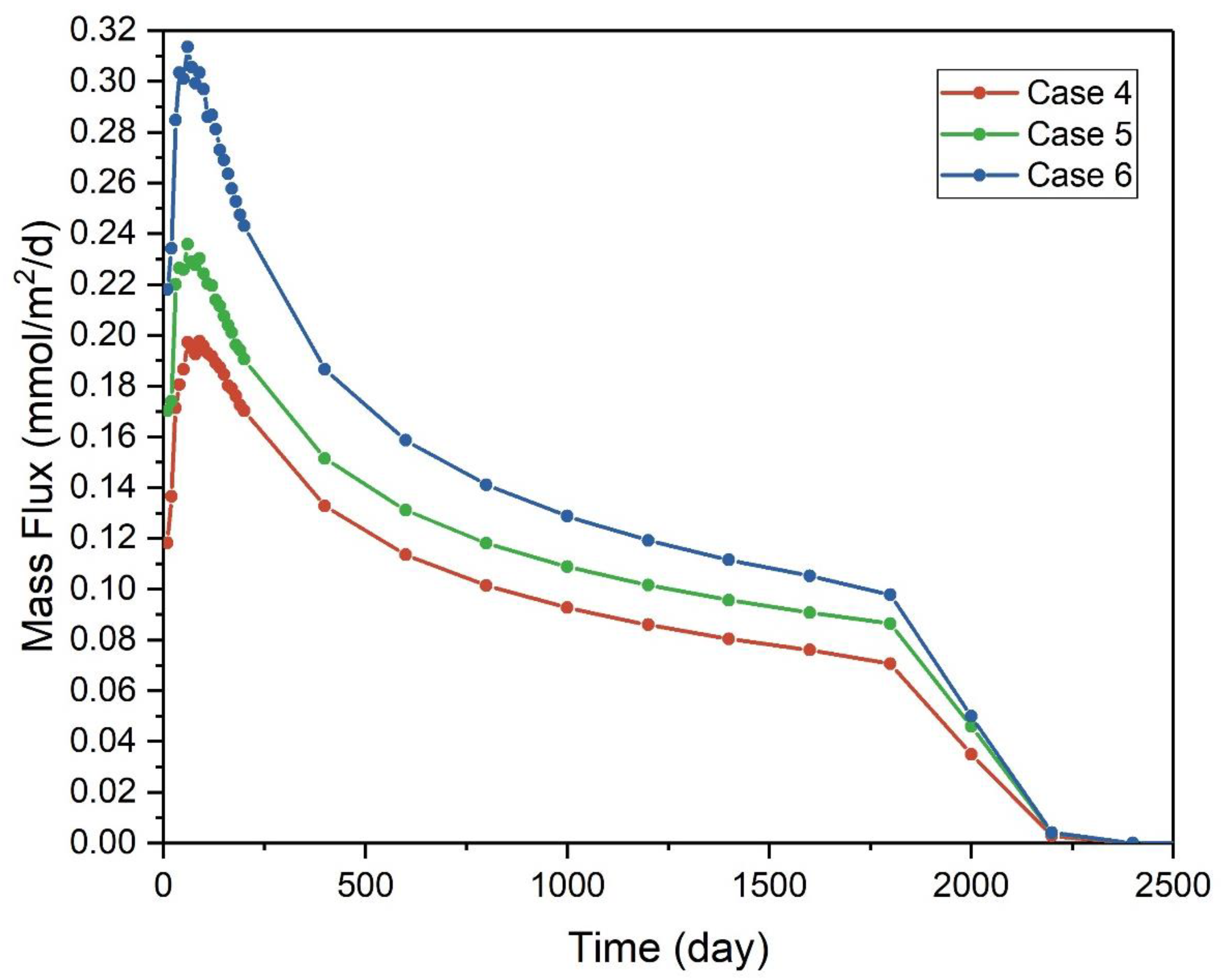
To further investigate how the maximum mass flux would be affected by the transverse dispersivity of the two-layer aquifer system, we recorded the time-varying maximum mass flux (Figure 6), while maintaining the same aquifer properties as in Section 3.4.1. Our observations revealed some interesting findings based on Figure 6. Firstly, increasing the transverse dispersivity of either layer led to an increase in the maximum mass flux. Secondly, regardless of any changes in the transverse dispersivity of either layer, the time required to complete the flushing process remained the same. Specifically, for Cases 4–6, it took approximately 2400 days to complete the flushing process.
The first observation supported the findings in Section 3.4.1 because an increase in the transverse dispersivity led to a higher hydrodynamic dispersion along the y-direction, thereby enhancing the mass flux across the interface of the two layers. The second observation revealed that the transverse dispersivity solely affected mass transfer in the vertical dimension. The constancy of the time required to complete the flushing process supports this result.
3.4.3. Effect of Transverse Dispersivity on Total Vertical Mass Flux
In Figure 5, the areas beneath the curves and the x-axis collectively represent the total vertical mass flux across the interface of two layers at a given time. To further investigate the total mass flux over time in different cases, we recorded the time-varying total mass flux, as depicted in Figure 7, while maintaining consistent aquifer properties as detailed in Section 3.4.1. Our observations yield noteworthy insights based on Figure 7. Firstly, all three curves exhibited an initial increase, culminating at their zenith (t = 1000 d), followed by a subsequent decline until the total mass flux reached zero. Secondly, prior to reaching zero, the total mass flux of Case 4 was consistently the smallest, while Cases 6 consistently exhibited the largest value. For example, the peak total mass flux for Case 4 was 3.767 mmol, for Case 5, it was 4.163 mmol, and for Case 6, it was 5.253 mmol.
A few points are notable for understanding the above observations. First, the total vertical mass flux depended on two factors: the vertical concentration gradient which determines the mass flux rate (per unit area) (which has been discussed in details in Section 3.4.1) and the total area used for conducting the vertical mass flux (which appears to be a dominating factor for controlling the total vertical mass flux). For a given unit width (along the horizontal direction perpendicular to the x-axis), the total area used for conducting the vertical mass flux was primarily controlled by the distance between the flushing front between layer-1 (which had a higher flushing velocity) and layer-2 (which had a lower flushing velocity), with limited horizontal dispersive zones near the two flushing fronts. At the beginning of the flushing process, the distance between the flushing front between layer-1 and layer-2 continuously increased with time; therefore, one will observe a continuously increasing total vertical mass flux. When the flushing front of the layer-1 reached the right boundary and exited the domain of concern, the distance between the flushing front between layer-1 and layer-2 reached its maximum, leading to the maximum total vertical mass flux. After this moment, the distance between the flushing of layer-2 and the right exit boundary will continuously decrease with time, leading to the decline of the total vertical mass flux. When the flushing front of layer-2 also reached the right exit boundary, the area for conducting the vertical mass flux was almost zero (with a limited horizontal dispersive zone around the flushing front); thus, the total mass flux will approach zero after this moment. The second observation serves as further evidence that an increase in transverse dispersivity corresponded to heightened hydrodynamic dispersion along the y-direction, consequently augmenting mass flux across the interface of the two layers.
3.5. Effect of Retardation Factor
The retardation factor plays a crucial role in influencing the flushing process and mass exchange across the interface. For a given Darcian velocity (q), the advective velocity of solute, denoted as vc, with a retardation factor R and a porosity of θ is
and the advective velocity is directly related to the movement of flushing front in either layer. Since the advective velocity is controlled by the product of R and θ in Equation (3), not by R or θ alone, the effect of the retardation factor would be akin to that of porosity. For instance, for a given θ value, doubling the R value and keeping the θ value unchanged will have the same advective velocity of solute as the case of doubling the θ value but keeping the R value unchanged.
An increase in the retardation factor of layer-2 yielded some interesting observations. Firstly, the peak value of mass flux at a given time would increase. Secondly, the range of mass flux would become wider, with the rising limb of the vertical mass flux-distance curve shifting toward the left boundary and the falling limb of the same curve remaining unchanged. Thirdly, the total mass exchanged between the two layers would increase. Moreover, the maximum mass flux during the entire flushing process would also be greater, and an increase in the retardation factor of layer-2 would prolong the time required for completing the flushing process.
Conversely, an increase in the retardation factor of layer-1 would result in a reduction in the peak mass flux at a given time. Secondly, the range of mass flux would become narrower, with the rising limb of the mass flux-distance curve remaining fixed and the falling limb of the same curve shifting to the left. Thirdly, there would be less mass flux across the interface at a given time. Finally, the curves would require similar times to complete the flushing process despite having varying retardation factors of layer-1. The explanation of the above observations is similar to what has been stated when discussing the porosity effect in Section 3.3.
4. Applications and Limitations
4.1. Applications
One of the most effective methods of cleaning contaminated groundwater is flushing with solute-free clean water. The application of flushing is typically used in layered heterogeneous aquifers where the primary groundwater flow direction is parallel to the layering of the aquifer. The flushing process can be monitored by measuring the concentration of the contaminants in the discharged water, which can be used to determine the effectiveness of the flushing process.
Another benefit of flushing with solute-free clean water is that it is a relatively low-cost method of remediation. Unlike other methods of remediation, such as pump-and-treat or in situ treatment, flushing with solute-free clean water requires little equipment and can be implemented quickly. This means that the cost of the remediation is significantly reduced, making it an attractive option for communities and industries that need to clean contaminated groundwater.
4.2. Limitations and Future Works
While flushing with solute-free clean water is an effective method of remediation, there are some limitations to its use. One of the primary limitations is that it is only effective in heterogeneous aquifers where the flow direction is parallel to the layering of the aquifer. In other types of aquifers, such as fractured or karst aquifers, the flushing process may be less effective or not effective at all. The study only considered rather simple geochemical processes such as inhibition. Complex biogeochemical reactions were not considered and should be explored in the future. The discussed flushing method may also not be effective for all types of contaminants as well. For example, some contaminants, such as heavy metals, may not be easily removed by flushing with solute-free clean water. In these cases, alternative methods of remediation may be necessary.
Secondly, the conceptual model used in this study was rather simple, and so, the result may be limited. For example, we assumed that each layer was homogeneous. When aquifer heterogeneity prevails, particularly when clay and silt lenses exist in the layer, the efficiency of flushing will drop because the trapped contaminants in those lenses cannot be easily flushed out due to the much slower groundwater flow velocity there.
Finally, the problem discussed here has no available analytical solution to benchmark the developed numerical solution. We conducted extensive numerical exercises using different meshes to ensure that the numerical errors due to discretization are negligible. We also used very fine meshes to ensure that the numerical dispersion and numerical oscillation are not a concern when using the COMSOL Multiphysics platform to perform the simulations. However, the theoretical work of this investigation has not been validated by experimental data, which are not available at present. Those experiments are important for testing the flushing theory and should be conducted in the future.
5. Conclusions
In this study, we used a two-layer heterogeneous aquifer system as an example to investigate how the porosity, transverse dispersivity, and retardation factor would affect the flushing of solute from an originally contaminated porous media system. We developed a high-fidelity 2-D finite-element numerical model in the COMSOL Multiphysics platform to describe solute transport in the two-layer aquifer system taking into account the situation where water in both regions is mobile with different advective velocities. The transport of solutes in both layers was governed by the 2-D ADEs and was coupled by the continuity of concentration and mass fluxes across the interface between the two layers. The water flow was assumed to be steady state. The vertical mass flux mentioned below refers specifically to the vertical mass flux across the interface of two layers, if not explained otherwise. The primary conclusions can be summarized as follows:
- (1)
- With all the other parameters remaining the same, increasing the porosity of layer-2 (which has a slower flushing velocity) would (a) lead to increased mass flux across the interface of two layers, (b) shift the rising limb of the mass flux-distance curve towards the left boundary where solute-free water is introduced for flushing, resulting in a larger mass flux range at a given time. Thus, the total amount of mass flux at a given time would be greater. However, if keeping all parameter unchanged but increasing the porosity of layer-1 (which has a faster flushing velocity) would (a) lead to decreased mass flux, (b) shift the falling limb of the mass flux-distance curve towards the left boundary, causing less total mass flux. Furthermore, increasing the porosity of layer-2 would also prolong the time required for completely flushing out the solute from the system.
- (2)
- When increasing the transverse dispersivity in either layer-1 or layer-2, the mass flux would increase. Changing the transverse dispersivity has little effect on the longitudinal transport, and so, the time needed for completing the flushing process will not be affected.
- (3)
- Retardation factor plays a similar role with porosity. When all the other parameters remain unchanged, the increased retardation factor of layer-2 would increase the mass flux and expand the spatial range (along the layering or bedding direction) of the vertical mass flux. In contrast, an increased retardation factor in layer-1 would decrease the mass flux and lead to a reduced range of the vertical mass flux. Furthermore, increasing the retardation factor of layer-2 would also prolong the time needed for completely flushing out the solute from the system.
Author Contributions
Conceptualization, Z.C. and H.Z.; methodology, Z.C.; software, Z.C.; investigation, Z.C. and H.Z.; writing—original draft preparation, Z.C.; writing—review and editing, Z.C. and H.Z. All authors have read and agreed to the published version of the manuscript.
Funding
This research received no external funding.
Data Availability Statement
Data is contained within the article.
Acknowledgments
The authors would like to thank the Assistant Editor and the anonymous reviews for their constructive comments which helped us improve the quality of the manuscript.
Conflicts of Interest
The authors declare no conflict of interest.
References
- Chakraborti, D.; Rahman, M.M.; Mukherjee, A.; Alauddin, M.; Hassan, M.; Dutta, R.N.; Pati, S.; Mukherjee, S.C.; Roy, S.; Quamruzzman, Q. Groundwater arsenic contamination in Bangladesh—21 Years of research. J. Trace Elem. Med. Biol. 2015, 31, 237–248. [Google Scholar] [CrossRef]
- Wang, D.; Wu, J.; Wang, Y.; Ji, Y. Finding high-quality groundwater resources to reduce the hydatidosis incidence in the Shiqu County of Sichuan Province, China: Analysis, assessment, and management. Expo. Health 2020, 12, 307–322. [Google Scholar] [CrossRef]
- Su, Z.; Wu, J.; He, X.; Elumalai, V. Temporal changes of groundwater quality within the groundwater depression cone and prediction of confined groundwater salinity using Grey Markov model in Yinchuan area of northwest China. Expo. Health 2020, 12, 447–468. [Google Scholar] [CrossRef]
- Li, P.; Karunanidhi, D.; Subramani, T.; Srinivasamoorthy, K. Sources and consequences of groundwater contamination. Arch. Environ. Contam. Toxicol. 2021, 80, 1–10. [Google Scholar] [CrossRef]
- Tatti, F.; Papini, M.P.; Torretta, V.; Mancini, G.; Boni, M.R.; Viotti, P. Experimental and numerical evaluation of Groundwater Circulation Wells as a remediation technology for persistent, low permeability contaminant source zones. J. Contam. Hydrol. 2019, 222, 89–100. [Google Scholar] [CrossRef] [PubMed]
- Padhye, L.P.; Srivastava, P.; Jasemizad, T.; Bolan, S.; Hou, D.; Sabry, S.; Rinklebe, J.; O’Connor, D.; Lamb, D.; Wang, H. Contaminant containment for sustainable remediation of persistent contaminants in soil and groundwater. J. Hazard. Mater. 2023, 455, 131575. [Google Scholar] [CrossRef] [PubMed]
- Ibrahim, M.; Nawaz, M.H.; Rout, P.R.; Lim, J.-W.; Mainali, B.; Shahid, M.K. Advances in Produced Water Treatment Technologies: An In-Depth Exploration with an Emphasis on Membrane-Based Systems and Future Perspectives. Water 2023, 15, 2980. [Google Scholar] [CrossRef]
- Alazaiza, M.Y.; Albahnasawi, A.; Ali, G.A.; Bashir, M.J.; Copty, N.K.; Amr, S.S.A.; Abushammala, M.F.; Al Maskari, T. Recent advances of nanoremediation technologies for soil and groundwater remediation: A review. Water 2021, 13, 2186. [Google Scholar] [CrossRef]
- Hadley, P.W.; Newell, C.J. Groundwater remediation: The next 30 years. Groundwater 2012, 50, 669–678. [Google Scholar] [CrossRef]
- Reddy, K.R. Physical and chemical groundwater remediation technologies. In Overexploitation and Contamination of Shared Groundwater Resources; Springer: Berlin/Heidelberg, Germany, 2008; pp. 257–274. [Google Scholar] [CrossRef]
- Sharma, P.K.; Mayank, M.; Ojha, C.; Shukla, S. A review on groundwater contaminant transport and remediation. ISH J. Hydraul. Eng. 2020, 26, 112–121. [Google Scholar] [CrossRef]
- Mackay, D.M.; Cherry, J.A. Groundwater contamination: Pump-and-treat remediation. Environ. Sci. Technol. 1989, 23, 630–636. [Google Scholar] [CrossRef]
- Palmer, C.D.; Fish, W. Chemical Enhancements to Pump-and-Treat Remediation. In Epa Environmental Engineering Sourcebook; Superfund Technology Support Center for Ground Water, Robert S. Kerr Environmental Research Laboratory: Ada, OK, USA, 1992; pp. 59–86. [Google Scholar]
- Voudrias, E. Pump and treat remediation of groundwater contaminated by hazardous waste: Can it really be achieved. Glob. Netw. Environ. Sci. Technol. 2001, 3, 1–10. Available online: https://journal.gnest.org/sites/default/files/Journal%20Papers/voudrias.pdf (accessed on 11 September 2023).
- Rittmann, B.E.; Seagren, E.; Wrenn, B.A. In Situ Bioremediation, 2nd ed.; Elsevier Science: New York, NY, USA, 1994. [Google Scholar]
- Raymond, R.L.; Brown, R.A.; Norris, R.D.; O’neill, E.T. Stimulation of Biooxidation Processes in Subterranean Formations. U.S. Patent No. 4,588,506, 13 May 1986. [Google Scholar]
- Farhadian, M.; Vachelard, C.; Duchez, D.; Larroche, C. In situ bioremediation of monoaromatic pollutants in groundwater: A review. Bioresour. Technol. 2008, 99, 5296–5308. [Google Scholar] [CrossRef] [PubMed]
- Liu, D.; Li, Q.; Liu, E.; Zhang, M.; Liu, J.; Chen, C. Biomineralized nanoparticles for the immobilization and degradation of crude oil-contaminated soil. Nano Res. 2023, 1–8. [Google Scholar] [CrossRef]
- Park, M.; Wu, S.; Lopez, I.J.; Chang, J.Y.; Karanfil, T.; Snyder, S.A. Adsorption of perfluoroalkyl substances (PFAS) in groundwater by granular activated carbons: Roles of hydrophobicity of PFAS and carbon characteristics. Water Res. 2020, 170, 115364. [Google Scholar] [CrossRef]
- Bin Jusoh, A.; Cheng, W.; Low, W.; Nora’aini, A.; Noor, M.M.M. Study on the removal of iron and manganese in groundwater by granular activated carbon. Desalination 2005, 182, 347–353. [Google Scholar] [CrossRef]
- Liu, C.J.; Werner, D.; Bellona, C. Removal of per-and polyfluoroalkyl substances (PFASs) from contaminated groundwater using granular activated carbon: A pilot-scale study with breakthrough modeling. Environ. Sci. Water Res. Technol. 2019, 5, 1844–1853. [Google Scholar] [CrossRef]
- National Research Council. Alternatives for Ground Water Cleanup; National Academies Press: Washington, DC, USA, 1994.
- US EPA. Guidance on Remedial Actions for Contaminated Ground Water at Superfund Sites; Environmental Protection Agency: Washington, DC, USA, 1988.
- Chen, Z.; Wang, Y.; Zhan, H. Universal Relationship Between Mass Flux and the Properties of Layered Heterogeneity on the Contaminant Flushing Process. In Proceedings of the AGU Fall Meeting Abstracts, New Orleans, LA, USA, 13–17 December 2021. [Google Scholar]
- Barry, D.; Parker, J. Approximations for solute transport through porous media with flow transverse to layering. Transp. Porous Media 1987, 2, 65–82. [Google Scholar] [CrossRef]
- Anderson, J.L.; Bouma, J. Water movement through pedal soils: I. Saturated flow. Soil Sci. Soc. Am. J. 1977, 41, 413–418. [Google Scholar] [CrossRef]
- Vogel, H.-J.; Roth, K. Moving through scales of flow and transport in soil. J. Hydrol. 2003, 272, 95–106. [Google Scholar] [CrossRef]
- Tang, D.H.; Frind, E.O.; Sudicky, E.A. Contaminant transport in fractured porous media: Analytical solution for a single fracture. Water Resour. Res. 1981, 17, 555–564. [Google Scholar] [CrossRef]
- Chen, K.; Zhan, H. A Green’s function method for two-dimensional reactive solute transport in a parallel fracture-matrix system. J. Contam. Hydrol. 2018, 213, 15–21. [Google Scholar] [CrossRef]
- Tan, J.; Cheng, L.; Rong, G.; Zhan, H.; Quan, J. Multiscale roughness influence on hydrodynamic heat transfer in a single fracture. Comput. Geotech. 2021, 139, 104414. [Google Scholar] [CrossRef]
- Zhan, H.; Wen, Z.; Gao, G. An analytical solution of two-dimensional reactive solute transport in an aquifer-aquitard system. Water Resour. Res. 2009, 45, W10501. [Google Scholar] [CrossRef]
- Zeng, C.-F.; Xue, X.-L.; Zheng, G.; Xue, T.-Y.; Mei, G.-X. Responses of retaining wall and surrounding ground to pre-excavation dewatering in an alternated multi-aquifer-aquitard system. J. Hydrol. 2018, 559, 609–626. [Google Scholar] [CrossRef]
- Filippini, M.; Parker, B.L.; Dinelli, E.; Wanner, P.; Chapman, S.W.; Gargini, A. Assessing aquitard integrity in a complex aquifer–aquitard system contaminated by chlorinated hydrocarbons. Water Res. 2020, 171, 115388. [Google Scholar] [CrossRef]
- Hendrickx, J.M.; Flury, M. Uniform and preferential flow mechanisms in the vadose zone. In Conceptual Models of Flow Transport in the Fractured Vadose Zone; National Academies Press: Washington, DC, USA, 2001; pp. 149–187. [Google Scholar]
- Gerke, H.H. Preferential flow descriptions for structured soils. J. Plant Nutr. Soil Sci. 2006, 169, 382–400. [Google Scholar] [CrossRef]
- Coats, K.H.; Smith, B.D. Dead-end pore volume and dispersion in porous media. Soc. Pet. Eng. J. 1964, 4, 73–84. [Google Scholar] [CrossRef]
- Van Genuchten, M.T.; Wierenga, P.J. Mass transfer studies in sorbing porous media I. Analytical solutions. Soil Sci. Soc. Am. J. 1976, 40, 473–480. [Google Scholar] [CrossRef]
- Gao, G.; Zhan, H.; Feng, S.; Fu, B.; Ma, Y.; Huang, G. A new mobile-immobile model for reactive solute transport with scale-dependent dispersion. Water Resour. Res. 2010, 46, W08533. [Google Scholar] [CrossRef]
- Dou, Z.; Tang, S.; Zhang, X.; Liu, R.; Zhuang, C.; Wang, J.; Zhou, Z.; Xiong, H. Influence of shear displacement on fluid flow and solute transport in a 3D rough fracture. Lithosphere 2021, 2021, 1569736. [Google Scholar] [CrossRef]
- Blackmore, S.; Pedretti, D.; Mayer, K.; Smith, L.; Beckie, R. Evaluation of single-and dual-porosity models for reproducing the release of external and internal tracers from heterogeneous waste-rock piles. J. Contam. Hydrol. 2018, 214, 65–74. [Google Scholar] [CrossRef] [PubMed]
- Wood, B.D.; Dawson, C.N.; Szecsody, J.E.; Streile, G.P. Modeling contaminant transport and biodegradation in a layered porous media system. Water Resour. Res. 1994, 30, 1833–1845. [Google Scholar] [CrossRef]
- Skopp, J.; Gardner, W.R.; Tyler, E.J. Solute movement in structured soils: Two-region model with small interaction. Soil Sci. Soc. Am. J. 1981, 45, 837–842. [Google Scholar] [CrossRef]
- Gerke, H.H.; Van Genuchten, M.T. A dual-porosity model for simulating the preferential movement of water and solutes in structured porous media. Water Resour. Res. 1993, 29, 305–319. [Google Scholar] [CrossRef]
- Liang, X.; Zhang, Y.K.; Liu, J.; Ma, E.; Zheng, C. Solute transport with linear reactions in porous media with layered structure: A semianalytical model. Water Resour. Res. 2019, 55, 5102–5118. [Google Scholar] [CrossRef]
- Wu, M.-C.; Hsieh, P.-C. Analytical modeling of solute transport in a two-zoned porous medium flow. Water 2022, 14, 323. [Google Scholar] [CrossRef]
- Kurasawa, T.; Takahashi, Y.; Suzuki, M.; Inoue, K. Laboratory Flushing Tests of Dissolved Contaminants in Heterogeneous Porous Media with Low-Conductivity Zones. Water Air Soil Pollut. 2023, 234, 240. [Google Scholar] [CrossRef]
- Dorchester, L.; Day-Lewis, F.D.; Singha, K. Evaluation of Dual Domain Mass Transfer in Porous Media at the Pore Scale. Groundwater 2023. [Google Scholar] [CrossRef]
- Chen, Z. Flushing of Contaminated Homogenous and Heterogenous Aquifers. Master’s Thesis, Texas A&M University, College Station, TX, USA, 26 April 2021. [Google Scholar]
Figure 1.
Schematic diagram of a flushing model in the layered heterogeneous aquifer. The thickness of the layer is denoted as B, L is the length of domain, and the subscripts 1 and 2 represent the parameters in layer-1 and layer-2, respectively.
Figure 1.
Schematic diagram of a flushing model in the layered heterogeneous aquifer. The thickness of the layer is denoted as B, L is the length of domain, and the subscripts 1 and 2 represent the parameters in layer-1 and layer-2, respectively.

Figure 2.
The concentration distributions at different times (50th, 200th, 600th, 1000th days).

Figure 3.
The vertical mass flux of Cases 1–3 between the layers varies with distance at different times. (a) Case 1; (b) Case 2; (c) Case 3; (d) An example curve (Case 1 at t = 600 d) with turning points highlighted.
Figure 3.
The vertical mass flux of Cases 1–3 between the layers varies with distance at different times. (a) Case 1; (b) Case 2; (c) Case 3; (d) An example curve (Case 1 at t = 600 d) with turning points highlighted.

Figure 4.
The maximum mass flux over time of Cases 1–3 across the interface of two layers.

Figure 5.
The vertical mass flux of Cases 4–6 across the interface of the layers varies with distance at different times. (a) Case 4; (b) Case 5; (c) Case 6.
Figure 5.
The vertical mass flux of Cases 4–6 across the interface of the layers varies with distance at different times. (a) Case 4; (b) Case 5; (c) Case 6.

Figure 6.
The maximum mass flux over time of Cases 4–6 across the interface of two layers.

Figure 7.
The total vertical mass flux over time of Cases 4–6 across the interface of two layers.


Table 1.
Summary of the latest relevant studies including their approaches, main focuses, and differences from this investigation.
Table 1.
Summary of the latest relevant studies including their approaches, main focuses, and differences from this investigation.
| Literatures | Methods | Main Points | Differences from This Study |
|---|---|---|---|
| [44] | Semi-analytical model | The model considers transverse dispersion and linear reactions in a layered medium, and the mass exchange between the zones is determined by the transverse dispersion across the interface. | This paper focused only on the transverse dispersion but did not consider other influence factors. |
| [45] | Analytical model | The modeling results show that the pollutant concentration is more sensitive to the Peclet number than the retardation factor and the first-order decaying coefficient in uniform groundwater flow. | The model was based on 1-D ADE, and the flow direction was perpendicular to the interface of two layers. |
| [46] | Laboratory model | The effects of the geometry of low-conductivity zones, conductivity contrast, and flow regime on solute flushing. | This paper focused only on the conductivity contrast but did not consider other influence factors. |
| [47] | Synthetic pore-scale millifluidics simulation | They compared the length scales associated with mass transfer rate and the calculation of the Peclet number and found that the Peclet number is commonly larger than the characteristic length scale associated with mass transfer rate. | The simulations were using a millifluidics device, which might not fully represent the complex and heterogeneous nature of real-world porous media. |
Table 2.
Different porosities of conceptual Cases 1–3.
| Case No. | θ1 | θ2 |
|---|---|---|
| 1 | 0.1 | 0.2 |
| 2 | 0.1 | 0.4 |
| 3 | 0.2 | 0.4 |
Table 3.
Different transverse dispersivities of conceptual Cases 4–6.
| Case No. | αT1 | αT2 |
|---|---|---|
| 4 | 0.01 | 0.02 |
| 5 | 0.01 | 0.04 |
| 6 | 0.02 | 0.04 |
Disclaimer/Publisher’s Note: The statements, opinions and data contained in all publications are solely those of the individual author(s) and contributor(s) and not of MDPI and/or the editor(s). MDPI and/or the editor(s) disclaim responsibility for any injury to people or property resulting from any ideas, methods, instructions or products referred to in the content. |
© 2023 by the authors. Licensee MDPI, Basel, Switzerland. This article is an open access article distributed under the terms and conditions of the Creative Commons Attribution (CC BY) license (https://creativecommons.org/licenses/by/4.0/).
Share and Cite
MDPI and ACS Style
Chen, Z.; Zhan, H. Universal Relationship between Mass Flux and Properties of Layered Heterogeneity on the Contaminant-Flushing Process. Water 2023, 15, 3292. https://doi.org/10.3390/w15183292
AMA Style
Chen Z, Zhan H. Universal Relationship between Mass Flux and Properties of Layered Heterogeneity on the Contaminant-Flushing Process. Water. 2023; 15(18):3292. https://doi.org/10.3390/w15183292
Chicago/Turabian StyleChen, Zehao, and Hongbin Zhan. 2023. "Universal Relationship between Mass Flux and Properties of Layered Heterogeneity on the Contaminant-Flushing Process" Water 15, no. 18: 3292. https://doi.org/10.3390/w15183292
Note that from the first issue of 2016, this journal uses article numbers instead of page numbers. See further details here.