BTX Removal from Open Aqueous Systems by Modified Cellulose Fibers and Evaluation of Competitive Evaporation Kinetics


1
Department of Chemistry and Chemical Technologies, University of Calabria, 87036 Arcavacata di Rende (Cs), Italy
2
Department of Environmental Engineering, University of Calabria, 87036 Arcavacata di Rende (Cs), Italy
*
Authors to whom correspondence should be addressed.
Water 2020, 12(11), 3154; https://doi.org/10.3390/w12113154
Submission received: 20 October 2020
/
Revised: 7 November 2020
/
Accepted: 10 November 2020
/
Published: 11 November 2020
(This article belongs to the Special Issue Application of Biological and Chemical Processes to Wastewater Treatment)
Abstract
:BTX stands for Benzene, Toluene, and Xylenes, which are volatile organic compounds contained in petroleum products such as gasoline. They have negative health effects and are sadly known for soil, air, and water contamination. This paper provides an investigation on BTX removal from open water systems like those represented by natural water bodies. In such systems, the evaporation process takes place, stealing the pollutants from the aqueous matrix by transferring them into the air, resulting in a secondary pollution. To prevent this situation, adsorption of these organic compounds on cellulose fibers, extracted from Spanish Broom vegetable, was studied. Raw and surface modified cellulose fibers were used for this purpose. The second ones were hydrophobized by two different green and low-cost functionalization systems (no solvent urethane functionalization and low pressure plasma treatments). Batch experiments were performed in an open system where BTX underwent two competing removing mechanisms: volatilization, and adsorption/desorption on/from the fibers dispersed in the water system. A mathematical model was implemented for the interpretation of the observed time-varying pollutant concentrations and the estimation of the kinetic constants for adsorption, desorption, and evaporation. The developed model, provided with the aforementioned parameters calibrated for each type of fibers, was then used for the prediction of their adsorption capacities both into open and closed systems.
1. Introduction
Approximately 71% of the planet is covered by water. Most of this water (>97%) is stored in the oceans, while the rest lies in the polar ice-caps and glaciers. Continental freshwaters represent less than 1% of the total volume, and most of them are groundwater [1].
Therefore, only a very small amount of water is accessible to humans, which is used for domestic, agricultural, and industrial purposes [2]. In the last hundred years, water consumption has dramatically increased compared to the available resources and, at the same time, environmental pollution has contributed to worsen its quality [3].
Nowadays, one of the major environmental problems is the remediation of the polluted water bodies, by hazardous chemicals such as Hydrophobic and Volatile Organic Compounds (HOCs and VOCs) [4].
BTX indicates a group of mono-aromatic volatile organic compounds (VOCs), such as Benzene, Toluene, and Xylenes.
The application of BTX is strictly related to their characteristics and properties, which are very similar among such classes of compounds. In particular, the high evaporation rate, the poor reactivity, the absence of corrosion phenomena against metals, and the ability to quickly dissolve a wide range of organic compounds have led to a widespread use of these products, since the beginning of the last century, in various industrial sectors.
Today, most of the produced Benzene, Toluene, and Xylenes are used in the chemical sector as starting compounds to obtain several secondary products, such as plastics, resins, detergents, pesticides, intermediates for the pharmaceutical industry, paints, adhesives, and inks [6].
The major sources of water contamination, caused by mono-aromatic chemicals belonging to the BTX class, are wastewater discharge from industrial processes and chemical industries, release of petroleum products from the storage tanks, accidents associated with oil and gas spill activities and petroleum transportation, road pavement operations, tobacco smoke and solvents use, and vehicular, air, and maritime traffic [7,8,9].
Their high volatility indicates that the main route of exposure for humans is inhalation. These compounds are considered priority contaminants by different national and international institutions due to the high risk of exposure and the consequent dangerous effects on human health. In particular, exposure to BTX can cause irritation of skin, eyes, and mucous membranes, as well as serious and potentially fatal nervous system deficiencies, myelo-suppression, leukemia, and cancer [10,11].
According to the World Health Organization (WHO), Benzene is the most toxic and powerful carcinogen among BTX; indeed, it occupies the sixth place in the list of the most dangerous substances worldwide. Its dangerousness is related to the carcinogenic effects resulting from chronic exposure. In particular, it has been classified as a class A1 substance (substances for which there is a confirmed evidence of relation to cancer induction in humans) by the most important international agencies, including EPA (Environmental Protection Agency), I.A.R.C. (International Agency for Research on Cancer), WHO (World Health Organization), N.I.O.S.H. (National Institute for Occupational Safety and Health), and A.C.G.I.H. (American Conference of Governmental Industrial Hygienists) [10,11,12].
When BTX are released into the environment, evaporation processes generate dispersion into air, though high concentrations are also found in groundwater and surface water. Despite the high risk of contact and the consequent negative effects on human health, BTX compounds remain neglected and untreated in municipal water systems, thus increasing the risk of diseases related to their ingestion [4,9].
Recent studies, carried out on drinking water in the USA, have found maximum concentrations of benzene, toluene, and xylene of 0.005, 1, and 10 mg/L, respectively [13,14]. Additionally, BTX are most often found in municipal wastewater in the range of 0 to 933 μg/L (85.5 μg/L for toluene) [15]. The presence of these pollutants in municipal treatment plants may originate from small factories, utilities, and domestic wastewater [16,17]. A significant BTX concentration (around 3–4 μg/L) has been also found, during fermentation processes, in the liquor of the digested sludge treated inside primary settling tanks. It has been observed that, in the acidophilic phase of the fermentation, the concentration of toluene could increase up to 42,000 μg/L [18].
Due to the increase in the concentration of these mono-aromatic compounds in the environment, the scientific community is constantly looking for efficient and sustainable methodologies to mitigate this pollution.
Several technologies have been developed to remove BTX from polluted water bodies such as chemical degradation/oxidation processes including AOPs (advanced oxidation processes) [19], and heterogeneous photocatalysis with TiO2 mediated systems [20], which ensure almost the total degradation (>90%) of BTX concentration ranging from 1 to 20 mg/L and, in some cases, the removal of more than 80% of the phenolic intermediates in about 30 min [19]. Homogeneous photocatalysis studies, based on the Fenton reaction (photo-Fenton type: H2O2/UV) [21], show that initial concentrations of monoaromatic hydrocarbons of about 10 mg/L can be reduced, in the best cases, by about 80% after 150 min. Other methods like ozonation and electrochemical processes achieve removal efficiencies of over 90%, for BTEX concentrations from 1 to 10 mg/L [22,23,24,25], and biological demolition processes such as bioremediation and bioleaching [26,27] allow us to remove/degrade over 90% of the initial concentration (up to 50 mg/L of BTX) in 25 h. Physical methods such as air stripping [28,29] achieve a removal efficiency of more than 90% at a temperature of 50 °C and an air-water ratio of 100, while adsorption methods on activated carbon and zeolites [30,31] have an average removal efficiency higher than 90% for contact times of 72 h and an initial BTEX concentration of 100 mg/L. Unfortunately, these processes have limitations in terms of applicability, solid waste production and high costs.
In this regard, the adsorption of water-dissolved pollutants by means of natural fibers represent an effective alternative to the aforementioned methods. Cellulosic and lignocellulosic fibers [4,32,33,34,35,36,37,38] are cost-effective reagents resulting from the use of low-cost or waste materials. The high adsorbing capacity of these natural fibers is attributable to the presence of interfiber capillaries and a considerable specific surface area (SSA). Cellulosic fibers such as hemp, cotton, and flax have SSA in the range of 0.3 to 27.1 m2/g [39,40]. Cellulosic fibers, extracted from Spanish broom and used in this adsorption study, have a specific surface area of 1.3 m2/g, for what concerns raw fibers, and 1.4 m2/g for functionalized ones (the values were determined by the Brunauer–Emmett–Teller (BET-SSA) analysis). Such fibers exhibit a maximum adsorption capacity, towards Total Petroleum Hydrocarbons (TPH), higher than 200 mg/g. [4,36]. The absence of secondary products during their application and the possibility for their re-use several times imply a low environmental impact. Nevertheless, the biggest advantage lies in the possibility of fiber surface functionalization using sustainable methods: the presence of reactive hydroxyl groups emerging from the fiber surface [41] allows us to add specific functional sites (which correspond to the pollutant absorption sites), with the aim of increasing the affinity and/or selectivity of the adsorbent material for the contaminant to be removed from water [36,37,38,39,40,41].
Based on these considerations, this study presents the possibility to employ raw cellulose fibers and hydrophobized cellulose fibers (extracted from Spanish Broom (SB), a spontaneously growing shrub of the Mediterranean flora, largely diffuse even in other continents) [42,43], as sorbent materials to remove Benzene, Toluene, and Xylenes (BTX) from polluted water. The hydrophobic properties are obtained by two different green and low-cost functionalization processes: a urethane functionalization by a home-made still reactor and a low pressure plasma system.
The aim of the study is therefore to ascertain the possibility to use cellulose fibers for BTX removal from water. In particular, one of the most important aspects has been the study of the effect of fibers surface hydrophobization with respect to their adsorbing capabilities towards BTX. The estimation of the kinetic and thermodynamic parameters of the involved phenomena bringing to BTX remediation has been an objective as well. For these purposes, batch experiments were performed in an open system where BTX underwent two competing removing mechanisms: volatilization, and adsorption/desorption on/from the fibers dispersed in the aqueous system. A mathematical model was implemented for the interpretation of the measured time-varying pollutant concentrations, and the estimation of the kinetic constants for adsorption, desorption, and evaporation. The developed model, provided with the aforementioned parameters calibrated for each type of adopted fibers, was then used for the clear prediction of their adsorption capacities both into open and closed systems.
2. Materials and Methods
2.1. Raw Cellulose Fiber Extraction
The raw cellulose fibers (RF) were extracted from SB by using a pulping process of the vegetable in a 5% w/w NaOH solution. The vegetable was macerated for 20 min at a temperature of 80 °C. After this treatment, the cellulose fiber could be easily separated from the inner woody skeleton. Lignin impurities were removed by further washing the cellulose fibers with a 5% w/w NaOH solution at a temperature of 80 °C.
All chemicals used in this study were of analytical grade and without further modification. Benzene was purchased from Fluka Chemika (density d = 0.88 g/mL, purity = 99.5%, MW = 78.11 g/mol), toluene from Sigma-Aldrich (density d = 0.865 g/mL, purity = 99.7%, MW = 92.14 g/mol), xylenes from Riedel-de Haën (density d = 0.866 g/mL, purity = 99.6%, MW = 106.16 g/mol), and methanol from Sigma-Aldrich.
2.2. Hydrophobized Cellulose Fibers
The surface hydrophobization of the cellulosic fibers was carried out by using two different functionalization processes, as already reported previously [4,36].
The following adsorbent materials were prepared:
- 4,4′-diphenylmethane diisocyanate functionalized fiber (MDI-FF);
- Plasma Functionalized Fiber with low-pressure plasma technique (PFF).
The first functionalization method exploited the high reactivity of the isocyanate groups of the 4,4′-diphenylmethane diisocyanate molecule (4,4′-MDI), with the hydroxyl groups emerging from the surface of the fiber (Figure 1) [4].
Spectroscopic characterization analysis (such as X-ray photoelectron spectroscopy (XPS) and FT-IR) confirmed the presence of the urethane bond in the functionalized fiber. XPS analyses were performed with a Scanning XPS Microprobe (PHI 5000 Versa Probe II, Physical Electronics), equipped with a monochromatic Al Kα X-ray source (1486.6 eV), operated at 15 kV and 24.8 W, with a spot of 100 μm. FT-IR analysis was carried out with a Bruker ALPHA FT-IR spectrometer, provided with a A241/D reflection module, in the spectral range 375–4000 cm−1. The surface characterization analysis (such as SEM and water contact angle (WCA)) indicated the modification of the fiber surface, with an increase in the water contact angle from 75° (RF) to 148° for the functionalized fiber (MDI-FF), confirming the high hydrophobic character of the latter [4]. A LEO 420 scanning electron microscope (LEO Electron Microscopy Inc., New York, NY, USA), operating 15 kV, was used to observe the fibers, after metallization with sputtered gold–palladium. The EDS module was an INCAx–Sight Oxford Instruments (Vacuum conditions: 8 × 10⁻⁶ Torr, iProbe = 650 pA, Current = 15 kV). The water contact angle was measured through a manual goniometer Model 210 (Ramé-Hart Instrument Co., Succasunna, NJ, USA), utilizing 2 μL bi-distilled water drops deposited on stretched fibers.
The second functionalization method was conducted using a low-pressure plasma technique [36]. The process allowed the grafting of fluorinated groups on the fiber surface, by replacing the hydroxyl ones and/or the formation of new functional groups such as -OCF3, -OCF2, and -OCF2CF2 (Figure 2).
Additionally in this case, the spectroscopic and surface characterization analysis showed considerable differences between raw (RF) and functionalized fibers (PFF), with the latter displaying signals related to the presence of new functional groups on the fiber surface [36]. In particular, the high alkyl-fluorination level of the fiber surface led to a superhydrophobic PFF fiber (WCA >160).
2.3. BTX Analytical Determination
Benzene, toluene, and xylenes concentrations in aqueous solutions were measured according to the method by Bahrami et al., (2011) [44], by means of a high-performance liquid chromatography (HPLC) system (LC-20AD, Pump, Detector, Oven, Autosampler, Shimadzu, Tokyo, Japan) coupled with a diode array detector (Shimadzu). Samples were separated by reverse phase (RP) chromatography using a Discovery C18 Supelco column (5 μm, 15 cm × 3.0 mm). Briefly, BTX were eluted by a methanol/water (60/40, v/v) mobile phase at a flow rate of 1 mL/min, with an injection volume of 10 μL, and detected by a UV spectrophotometer at a wavelength of 254 nm. The calibration curve was prepared using the external standard method (BTX in MeOH), using solutions with different concentrations: 1, 2, 10, 50, and 150 ppm for each component.
Table 2 shows the analytical parameters of the calibration curves adopted for the quantification of BTX.
2.4. BTX Evaporation Experiments
BTX evaporation kinetics from the aqueous phase was evaluated in BTX aqueous solutions with an initial concentration set around 50 mg/L for each component. These solutions were shaken for 6 h to reach a complete mixing state, and then left to rest for 2 h in a closed flask. Finally, the solutions were poured into a glass beaker with 15.0 cm diameter and with 20.0 cm height. The liquid height from the beaker bottom was 7.5 cm. Solutions were constantly stirred at 100 rpm. BTX evaporation rates at room temperature were determined by analyzing their residual concentrations in solution at different times.
2.5. Batch Experiments for Water Purification
Analogous BTX solutions were used to study the competitive adsorption and volatilization mechanisms. In each experiment, 0.5 g of fiber was added to 200 mL of polluted aqueous solution, prepared as described above and maintained in continuous agitation under magnetic stirring at 100 rpm (Analog magnetic stirrer M2-A ArgoLab—Giorgio Bormac srl, Italy), in a beaker having the same dimensions as the one used in the volatilization experiment, in order to have constant evaporation conditions. Current concentrations of the pollutants were measured by sampling the solution at different contact times: 0, 3, 5, 10, 15, 30, 45, 60, and 120 min. Each time 1 mL of the solution was collected from the batch in a sealed HPLC vial and rapidly analyzed.
2.6. Mathematical Modeling
The contaminants taken into consideration in this study have rather high evaporation Henry constants (adimensional and expressed as the distribution ratio between the gas phase concentration and the liquid phase concentration: H’ Benzene = 2.27 × 10⁻¹; H’ Toluene = 2.71 × 10⁻¹; H’ Xylene = 2.12 × 10⁻¹) [45]. Therefore, the BTXs are volatile enough to be removed from the aqueous solution by the evaporation process. The release of these contaminants, from water to the surrounding environment, is facilitated precisely by this phenomenon. Studies have been directed toward the development of theoretical models with the aim of predicting the fate of volatile organic pollutants present in industrial wastewater [46]. Our experiments were performed in an open system where two phenomena are in competition with respect to the BTX removal from the aqueous phase: the evaporation into the air and the adsorption on the cellulose fibers. The system can be schematized as shown in Figure 3, and being the pollutants concentration into the aqueous phase and absorbed onto the fibers, respectively, while is the concentration lost by evaporation. In order to give a quantitative interpretation of the relative importance of the two mechanisms, a theoretical model taking both of them into account needs to be developed (Appendix A).
This model can be represented by the following differential equations:
under the constraints , where , , and are the adsorption, desorption, and evaporation kinetic constants, and is the pollutant concentration at time = 0.
The model is valid as long as the surface adsorbing sites of the fibers are in excess of the pollutant molecules in such a way that their number can be considered constant and can be included in .
2.6.1. Kinetic Model in Absence of the Adsorbing Fibers
In order to estimate the contribution of the evaporation process, on the kinetics of BTX removal in the blank experiments made in absence of adsorbing fibers, Equation (1) can be used under the condition and , that is to say, in the form of the single Equation (2):
which gives for a simple exponential trend:
2.6.2. Kinetic Interpretation in the Presence of Absorbing Fibers
In this case, the solution of the equation system 1, as it is shown in Appendix A, brings to the following relations:
3. Results and Discussion
Data collected during the evaporation experiments are displayed in Figure 4, which shows the trend of the normalized concentration of the BTX as a function of time, as well as their fit by the exponential function (Equation (3)). Table 3 shows the estimated values of the evaporation kinetic constants.
It can be seen that the experimental data agree quite well with the exponential trend predicted by Equation (3) (R2 ranges from 0.945 to 0.963), even if some systematic deviations can be observed at short sampling times. We believe that they are due to the evaporation process occurring during the time elapsed from sampling to pollutant concentration measurement. Despite any precaution taken to avoid evaporation phenomena, after sampling, some small amounts of the pollutants may indeed get lost during the required sample manipulations before measurements, thus leading to the measurement of slightly smaller concentrations than those actually expected at the time of sampling. This effect is particularly important at short sampling times, where evaporation is more effective due to the higher pollutant concentration. On the other hand, this effect is less visible in the case of samples containing the fibers (Figure 5) due to their competition in reducing the pollutants concentration in the solution: the faster this competition is, the lower the influence of this systematic error. In Figure 5, it can be seen that the deviation at short time is still present in the experiment related to the raw fibers (RF), even if to a lesser extent, but it is almost absent in the case of the functionalized ones (MDI-FF and PFF), where fiber adsorption is faster. Our kinetic model agrees with those of Mackay and Leinonen (1975) [47] and Chao et al. (2008) [48]. The evaporation constants are equal for the different BTX hydrocarbons, in the limit of the experimental error.
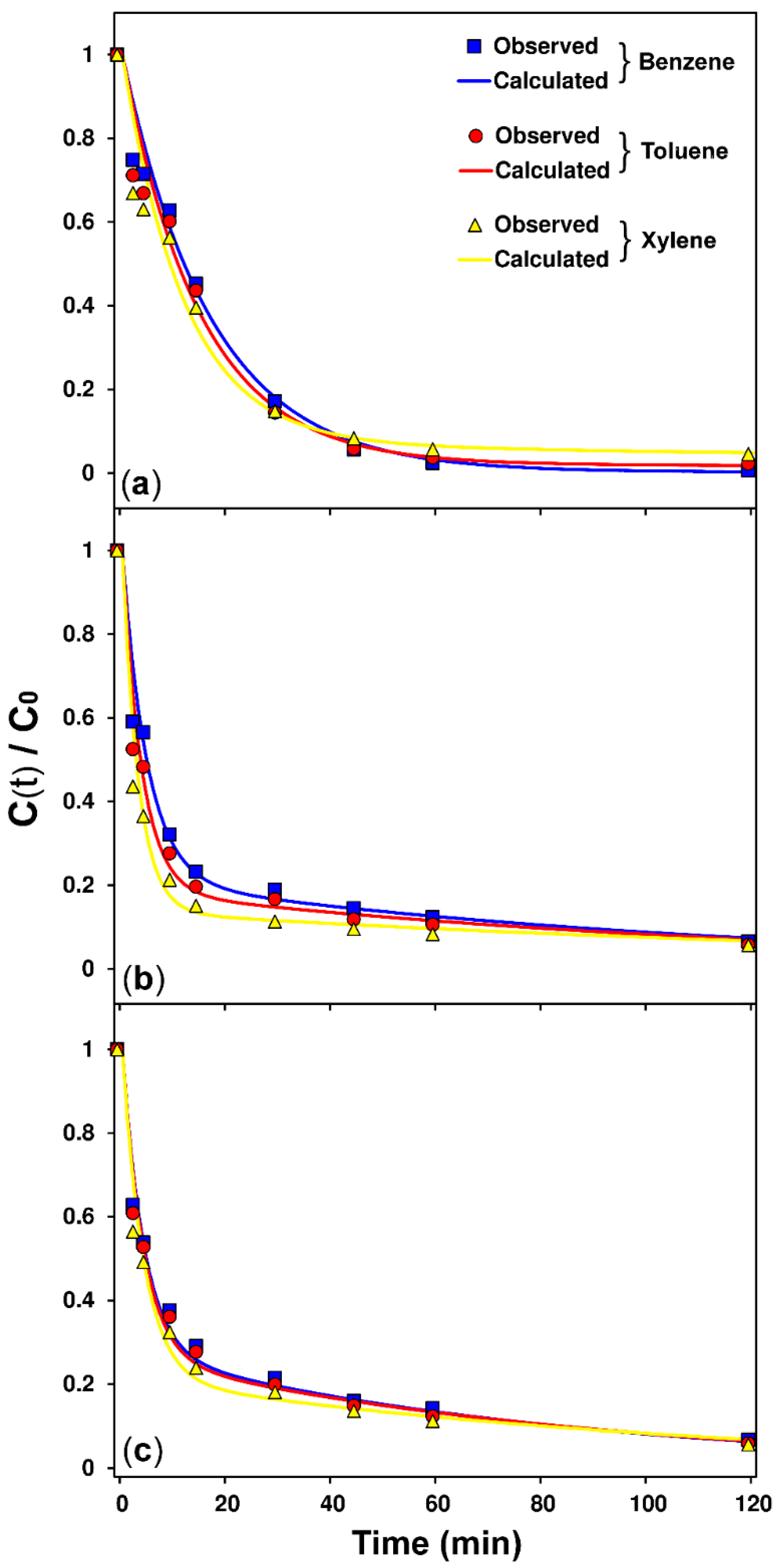
Fitting by Equation (4) of the experimental data measured during the adsorption tests for the three pollutants and the three different fibers, is illustrated in Figure 5, while the values of , , and , corresponding to best fits, are reported in Table 4.
The R2 of fitted data ranges from 0.97 to 0.99, indicating that Equation (4) gives a good representation of the experimental data (Figure 5).
It can be underlined that the values, estimated for the experiments in which the raw fibers (RF) was used as BTX adsorbent, are equal to those obtained in the blank experiment, the one in which only the evaporation process was at play. This gives good evidence that the kinetic model works quite well for the raw fibers. A discrepancy of the order of 20% is instead found between the evaporation kinetic constants obtained by fitting the data relative to the functionalized fibers (MDI-FF and PFF) experiments, with respect to that obtained from the blank experiment. In these cases, the model represented by Equation (1) does not work equally well. A straightforward way to explain the above discrepancies in is to consider that the surface hydrophobization does not preclude the possibility for BTX pollutants to be adsorbed on the sites already present on the raw fibers (RF) before functionalization. The model should be then modified to consider this second “cluster” of adsorption site. Of course, even maintaining the hypothesis of a first order kinetic, the new group of adsorption sites would introduce another equation, depending on two additional kinetic constants (adsorption and desorption), into the kinetic system (Equation (1)). This would lead to a complex model that could be solved only numerically, with eight experimental values of time-dependent pollutant concentrations that would not allow a reliable estimation of five independent kinetic parameters. An approximation, which can solve these issues in a very simple way, would be to consider only the adsorption process for these new sites, neglecting the desorption one. This approximation appears to be reasonable when considering that the desorption kinetic constant for the raw fibers is much smaller than the adsorption one (only about 4%; see Table 4). On the other hand, it seems reasonable to assume that the equilibrium constant for the above process is not affected by the functionalization. Raw fibers adsorption sites seem to be located below the outer surface, as will be discussed later. In this case, the kinetic model remains equal to that given by Equation (1), except for the introduction of the new term, , into the second member of the upper equation and related subsequent definitions,
being the adsorption kinetic constant for the second group of sites. All calculus equations remain the same as those shown above except for the substitution of with .
This means that the values of reported in Table 4, in the case of functionalized fibers (MDI-FF and PFF), represents the sum of the evaporation kinetic constant and the adsorption kinetic constant of the second group of sites. A fairly constant value (0.006–0.007 min−1) for this last parameter would explain the deviation of the calculated evaporation constants. One would expect that the value of this adsorption kinetic constant should be equal to that observed for in the row fiber experiments, but the reduced value can be attributed to the influence of the modified fiber surface. Work is in progress to investigate BTX behavior on the same fibers in closed systems, taking bigger amounts of data to confirm the applied model. We exclude, for the moment, failures of the model due to a restricted number of absorbing sites, which would bring to second order kinetic equations, due to the fact that data from raw fibers are very well interpreted in terms of a first order kinetics (the evaporation constant is equal to that derived for the blank experiment). Therefore, the hypothesis formulated to explain the discrepancies observed in the results obtained for the functionalized fibers, appears to be quite logic and consistent. Even if we have introduced the idea that a second cluster of adsorption site is present on the functionalized fibers, we will neglect the role of this site in the following discussion due to the smaller value of its absorption kinetic constants.
The values of , , and their ratio , representing the adsorption equilibrium constant, reported in Table 4 lead to some interesting considerations. It is somewhat surprising that the raw fiber (RF) shows the largest adsorption equilibrium constant for BTX. In the case of Benzene, it is one order of magnitude larger than that of the functionalized fibers (Table 4). The adsorption capacity of the raw fibers gradually decreases moving from Benzene to Toluene and Xylenes. The trend is reversed when looking at the adsorption equilibrium constant of the functionalized fibers.
This result is also surprising because the RF shows an adsorption equilibrium constant for total petroleum hydrocarbons, at least one order of magnitude smaller than that of the MDI-FF fiber [4]. In that paper, we showed that the raw fiber extracted from Spanish broom by the alkaline treatment is more hydrophobic (contact angle 75°) than pure cellulose (contact angle 40°) [49]. This is probably due to small percentages of lignin (2–3%) remaining trapped onto cellulose fibers during the alkaline digestion of vegetable, and subsequent washing processes [43,50,51]. The above residues could increase the affinity of the raw fiber, especially toward hydrophobic aromatic compounds like BTX, potentially explaining the above result. However, this issue needs support from experiments and will be the subject of further investigation.
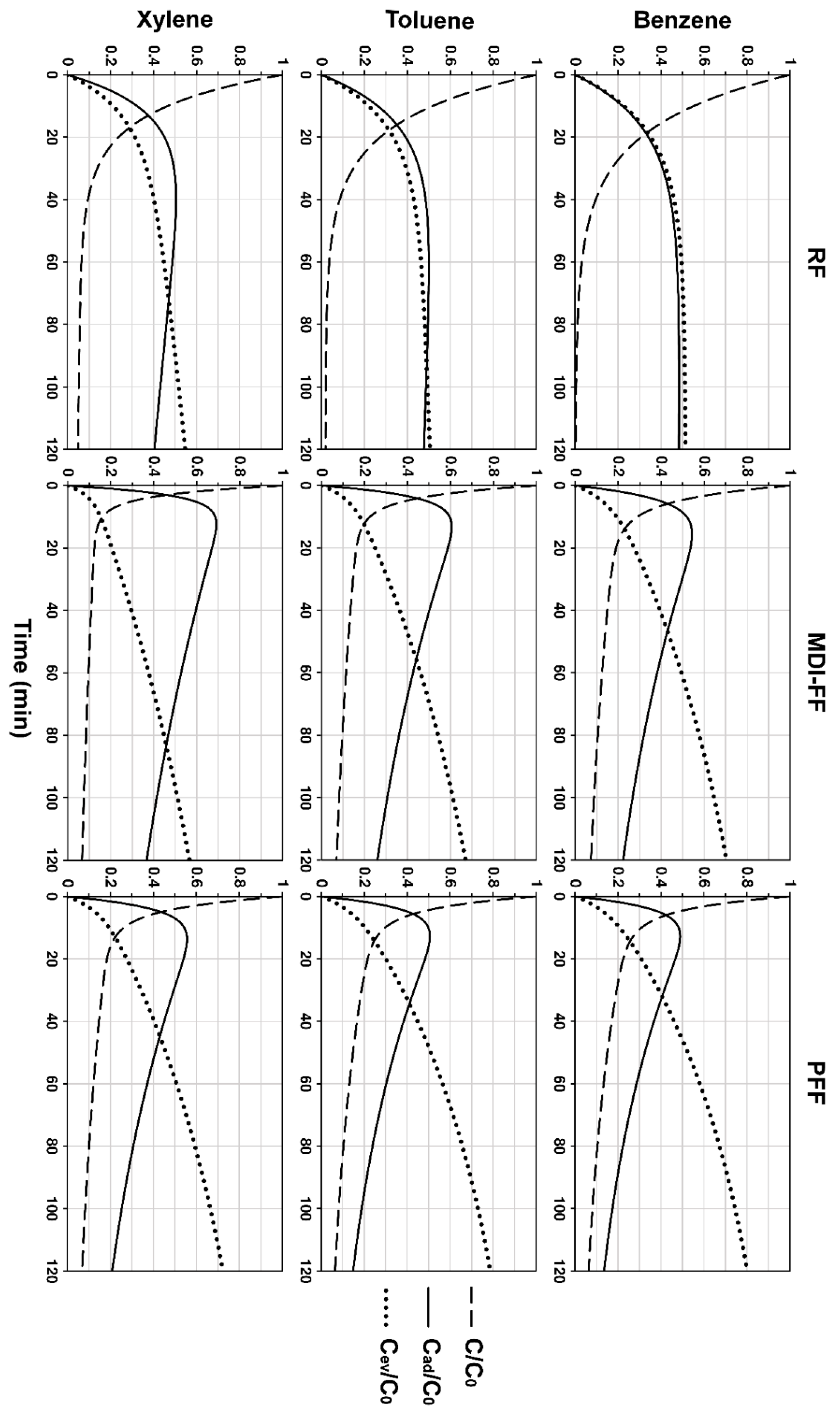
Anyway, it cannot be concluded that the raw fiber (RF) is a better adsorbent for BTX, at least in open systems where evaporation is a concomitant playing factor. Indeed, even if BTX adsorption on the raw fiber is thermodynamically favored, it loses importance when time competition between the adsorption and evaporation phenomena is taken into consideration. This competition is graphically illustrated in Figure 6, where the time variation of , (calculated by Equations (4) and (5)), and are reported. Of course, in an open system, all pollutants will evaporate from both the water and the fibers, but there will be a certain time at which the amount of the pollutants adsorbed on the fiber will have a maximum value (it is clearly seen in the graphs of Figure 6).
The time at which the maximum amount of adsorbed concentration is reached for each pollutant and each fiber is reported in Table 5, where the corresponding percentages of adsorbed, evaporated, and residual BTX concentration in solution are also shown.
MDI-FF is the fiber that has the best adsorption performances. It removes, if pulled out from the aqueous phase after only 13–16 min of contact time, 54.4%, 60.6%, and 69.1% of Benzene, Toluene, and Xylenes, respectively. After this time, the desorption process comes into play, returning the previously trapped pollutants to the aqueous phase. PFF is even faster than the MDI-FF (tmax = 13–14 min), but has much lower adsorption maxima. The RF is the last placed since the adsorption maxima are the lowest and their occurrence requires much more time.
As already mentioned, the experiments described in this paper deal with an open system, where the final fate of the pollutants dissolved in water is their complete extinction by evaporation. However, once the kinetic constants of the involved cellulose fibers have been estimated, it is possible to predict what would be the adsorption capacity of the same fibers, with respect to the three investigated pollutants, in a closed system where an equilibrium between the adsorbed species and those still dissolved in water would be reached after a certain time. These assumptions are certainly valid if referred to systems where the ratios between the amount of fibers and pollutant concentrations are maintained similar to those used in this work. In a closed system, where the volume filled by the gas phase is similar or lower with respect to that involved by the liquid phase, the amount of pollutants present in the gas phase can be neglected due to Raoult’s vapor tension law. Equation (1) can be then written as:
under the constraint:
Simple calculation shows that the pollutant concentration adsorbed by the fibers at equilibrium can be calculated by the equation:
while the time required to reach the equilibrium is given by:
The maximum percentages of pollutants that can be adsorbed at the equilibrium stage (%adseq), and the corresponding equilibrium time, in a closed polluted water system, can be calculated by using the two above Equations (12) and (13) (Table 6).
It is worth underlining that RF can absorb on average 91% of BTX, which corresponds, in the present case, to 54.6 milligrams of pollutants per gram of fiber, with an adsorption time of about 3.5 h. The MDI-FF shows an average adsorption of about 77%, which corresponds to 46.2 milligrams of BTX per gram of fiber, with an adsorption time no longer than 25 min. PFF adsorbs on average 67% of the pollutants, corresponding to an adsorption capacity of 40.2 milligrams of BTX per gram of fiber, for an adsorption time of 36 min.
This study shows that the functionalized fibers adsorb BTX with a fast kinetic. However, in an open system, fibers release the adsorbed BTX (Figure 5), so it can be thought that they can be more suitably applied in water remediation processes where they are cyclically purified from the adsorbed pollutants by some vacuum extraction and subsequently reused. In other words, they do not generate a waste after their employment. Furthermore, cellulosic fibers are very long living in water systems and their costs are relatively cheap (order of 1–2 euros/kg).
4. Conclusions
This work shows the first application of cellulosic fibers, extracted from Spartium Junceum vegetable species, for the purification of water polluted by BTX. Experiments were carried out in an open system where BTX would have the possibility to gradually leave the polluted water by evaporation. The development of an “ad hoc” mathematical model for the interpretation of the time-varying observed pollutants concentration allowed the estimation of the adsorption, desorption, and evaporation kinetic constants with respect to the cellulose fibers, as well as the prediction of their adsorption capacities both into open and closed systems. The adsorption behavior of the raw fiber was compared with that of the surface modified fibers, thus defined for the insertion of a hydrophobic surface. Surprisingly, the unmodified cellulose fiber showed the highest adsorption capacity for the BTX pollutants. This has been interpreted with the existence of a hydrophobic core under the surface of the fibers. This conclusion is based on the fact that the kinetic constants for adsorption and desorption of the raw fiber are much smaller than those of the functionalized ones. This observation seems to have a straightforward interpretation because the surface of the raw fiber is very hydrophilic and should provide a high activation barrier to the penetration of BTX hydrophobic molecules. The fiber functionalized by means of 4,4′-MDI (MDI-FF), appears to be the most convenient BTX adsorbent, since it has a slightly smaller adsorption capacity than the raw fibers, but a much faster adsorption kinetics (25 min instead of more than 3.5 h to reach the maximum adsorption). The plasma modified fiber, though superhydrophobic, shows the lowest affinity with BTX, probably because it does not have aromatic moieties. The results show that the 4,4′ MDI functionalized cellulosic fiber has efficient adsorbing properties against dissolved BTX in aqueous matrices. From an application point of view, it is possible that these functionalized fibers may find wide use in the purification of waste water deriving from petrochemical industrial activities, in which the concentration of the monitored contaminants is high and persistent.
Author Contributions
Conceptualization, A.T., F.C. and A.B.; methodology, F.C. and A.B.; software, A.T., F.C., R.B. and A.B.; validation, A.T., F.C. and A.B.; formal analysis, A.T., F.C., R.B. and A.B.; investigation, A.T., F.C., R.B. and A.B.; data curation, A.T., F.C., R.B. and A.B.; writing—original draft preparation, A.T. and R.B.; writing—review and editing, A.T., F.C. and A.B.; supervision, F.C. and A.B.; All authors have read and agreed to the published version of the manuscript.
Funding
This research was supported by University of Calabria in the framework of the ex 60% budget grant.
Acknowledgments
The authors would like to thank Nicoletta De Vietro and the Institute of Nanotechnology (Nanotec), National Research Council (CNR), c/o Department of Chemistry, University of Bari “Aldo Moro”, Italy, for providing the plasma functionalized fiber (PFF). The authors are also grateful to the Ministero dell’Istruzione dell’Università e della Ricerca Italiano (MIUR).
Conflicts of Interest
The authors declare no conflict of interest.
Appendix A
Reversible kinetic model of the adsorption and evaporation processes of VOCs dissolved into open aqueous systems
Using the annotations presented in the scheme of Figure 3 (see the article), it can be stated that:
where and are the water dissolved and the adsorbed pollutants concentrations, respectively, is the concentration lost by evaporation and is the pollutant concentration at time = 0.
The developed theoretical model giving a quantitative interpretation of the relative importance of both the adsorption and evaporation mechanisms is:
where , and are the adsorption, desorption and evaporation kinetic constants.
By setting and , Equation (A2) becomes:
using the following substitution:
the first order differential equations system turns into:
this system can be written in a matrix form:
in a vector form it becomes:
the solution for this kind of problems has the typical form:
the substitution of Equations (A8) into (A7) leads to:
where are the eigenvalues of matrix and are the associated eigenvectors. Equation (A9) can be written as follows:
Equation (A10) gives a solution only for those satisfying the following relation:
that is:
the determinant calculation leads to:
being (Equation (A4)), it gets to
the sum of the kinetic constants of the three processes at play becomes:
while the product
Equation (A16), therefore, becomes a second order equation with two solutions:
Once the eigenvalues are known, the eigenvectors can be determined using the solution of the differential equations system represented by Equation (A13). Using solution you get:
and then:
By multiplying the first row of the matrix by the column vector , which is the first solution associated with the first eigenvalue, one component of the vector can be expressed as a function of the other:
The component is a scalar whose value can be set equal to 1 without losing generality, since this last will be recovered when the solutions will be chosen as a linear combination of terms associated with the different calculated lambda values. The coefficients of this linear combination will be determined on the basis of the boundary conditions which will be specified below. Equation (A25) then becomes:
the second eigenvector can be obtained in a similar way using the solution :
by multiplying again the first row of the matrix by the column vector, you have:
and then:
similarly to what was done for the first solution, it arises
As previously said, the solutions of the of differential equations system will have the form of Equation (A8) and will be expressed by the following linear combination:
where and are the coefficients of the linear combination to be determined through the application of specific boundary conditions, relating to the system in which the processes take place. By substituting the terms obtained so far in Equation (A33) you have:
Equations (A35) and (A36) express the time variation laws of the water dissolved () and adsorbed () concentrations, respectively. By assigning the following boundary conditions:
Equations (A35) and (A36) become:
by developing this latter equation, you obtain:
by substituting Equation (A37) into the Equation (A39) you get:
can be determined using Equation (A37):
Finally, Equations (A35) and (A36) can be expressed as:
where:
References
- Li, X.; Wang, C.; Zhang, J.; Liu, J.; Liu, B.; Chen, G. Preparation and application of magnetic biochar in water treatment: A critical review. Sci. Total Environ. 2020, 711, 134847. [Google Scholar] [CrossRef]
- Sulaiman, A.A.; Attalla, E.; Sherif, M.A.S. Water Pollution: Source and Treatment. Am. J. Environ. Eng. 2016, 6, 88–98. [Google Scholar]
- Schweitzer, L.; Noblet, J. Water Contamination and Pollution. In Green Chemistry: An Inclusive Approach; Torok, B., Ed.; Elsevier: Cambridge, MA, USA, 2017; pp. 261–290. [Google Scholar]
- Tursi, A.; Beneduci, A.; Chidichimo, F.; De Vietro, N.; Chidichimo, G. Remediation of hydrocarbons polluted water by hydrophobic functionalized cellulose. Chemosphere 2018, 201, 530–539. [Google Scholar] [CrossRef] [PubMed]
- Mitra, S.; Roy, P. BTEX: A Serious Ground-water Contaminant. Res. J. Environ. Sci. 2011, 5, 394–398. [Google Scholar] [CrossRef] [Green Version]
- Speight, J.G. Heavy Oil Recovery and Upgrading; Elsevier BV: Amsterdam, The Netherlands, 2019; pp. 3–47. [Google Scholar]
- Alberici, R.M.; Zampronio, C.G.; Poppi, R.J.; Eberlin, M.N. Water solubilization of ethanol and BTEX from gasoline: On-line monitoring by membrane introduction mass spectrometry. Analyst 2002, 127, 230–234. [Google Scholar] [CrossRef] [Green Version]
- Costa, A.; Romão, L.P.C.; Araújo, B.; Lucas, S.; Maciel, S.; Wisniewski, A.; Alexandre, M. Environmental strategies to remove volatile aromatic fractions (BTEX) from petroleum industry wastewater using biomass. Bioresour. Technol. 2012, 105, 31–39. [Google Scholar] [CrossRef] [PubMed]
- Mazzeo, D.E.C.; Levy, C.E.; Angelis, D.D.F.D.; Marin-Morales, M.A. BTEX biodegradation by bacteria from effluents of petroleum refinery. Sci. Total Environ. 2010, 408, 4334–4340. [Google Scholar] [CrossRef]
- Akhbarizadeh, R.; Moore, F.; Keshavarzi, B.; Moeinpour, A. Aliphatic and polycyclic aromatic hydrocarbons risk assessment in coastal water and sediments of Khark Island, SW Iran. Mar. Pollut. Bull. 2016, 108, 33–45. [Google Scholar] [CrossRef]
- Wilbur, S.; Bosch, S. Interaction Profile for Benzene, Toluene, Ethylbenzene, and Xylenes (BTEX). Agency Toxic Subst. Dis. Regist. 2004. Available online: https://www.atsdr.cdc.gov/interactionprofiles/ip-btex/ip05.pdf (accessed on 11 November 2020).
- World Health Organization. Tobacco Smoke and Involuntary Smoking. In IARC Monographs on the Evaluation of Carcinogenic Risks to Humans; World Health Organization, International Agency for Research on Cancer: Lyon, France, 2004; Volume 83. [Google Scholar]
- Jodeh, S.; Ahmad, R.; Suleiman, M.; Radi, S.; Emran, K.M.; Salghi, R.; Warad, I.; Hadda, T.B. Kinetics, thermodynamics and adsorption of BTX removal from aqueous solution via date-palm pits carbonization using SPME/GC–MS. J. Ind. Eng. Chem. 2015, 6, 2853–2870. [Google Scholar]
- Daifullah, A.; Girgis, B. Impact of surface characteristics of activated carbon on adsorption of BTEX. Colloids Surf. A Physicochem. Eng. Asp. 2003, 214, 181–193. [Google Scholar] [CrossRef]
- Mrowiec, B. Effect of BTX on biological treatment of sewage. Environ. Prot. Eng. 2009, 35, 197–206. [Google Scholar]
- Bell, J.; Melcer, H.; Monteith, H.; Osinga, I.; Steel, P. Stripping of volatile organic compounds at full-scale municipal wastewater treatment plants. Water Environ. Res. 1993, 65, 708–716. [Google Scholar] [CrossRef]
- Namkung, E.; Rittman, B.E. Estimating volatile organic compound emission from publicly owned treatment works. J. Water Pollut. Control Fed. 1987, 59, 670–678. [Google Scholar]
- Roccotelli, A.; Araniti, F.; Tursi, A.; Simeone, G.D.R.; Rao, M.A.; Lania, I.; Chidichimo, G.; Abenavoli, M.R.; Gelsomino, A. Organic Matter Characterization and Phytotoxic Potential Assessment of a Solid Anaerobic Digestate Following Chemical Stabilization by an Iron-Based Fenton Reaction. J. Agric. Food Chem. 2020, 68, 9461–9474. [Google Scholar] [CrossRef]
- Tiburtius, E.R.L.; Peralta-Zamora, P.; Emmel, A. Treatment of gasoline-contaminated waters by advanced oxidation processes. J. Hazard. Mater. 2005, 126, 86–90. [Google Scholar] [CrossRef]
- De Vietro, N.; Tursi, A.; Beneduci, A.; Chidichimo, F.; Milella, A.; Fracassi, F.; Chatzisymeon, E.; Chidichimo, G. Photocatalytic inactivation of Escherichia coli bacteria in water using low pressure plasma deposited TiO2 cellulose fabric. Photochem. Photobiol. Sci. 2019, 18, 2248–2258. [Google Scholar] [CrossRef]
- Lhotský, O.; Krákorová, E.; Mašín, P.; Žebrák, R.; Linhartová, L.; Křesinová, Z.; Kašlík, J.; Steinová, J.; Rødsand, T.; Filipová, A.; et al. Pharmaceuticals, benzene, toluene and chlorobenzene removal from contaminated groundwater by combined UV/H2O2 photo-oxidation and aeration. Water Res. 2017, 120, 245–255. [Google Scholar] [CrossRef]
- Andreozzi, R. Advanced oxidation processes (AOP) for water purification and recovery. Catal. Today 1999, 53, 51–59. [Google Scholar] [CrossRef]
- Mascolo, G.; Ciannarella, R.; Balest, L.; Lopez, A. Effectiveness of UV-based advanced oxidation processes for the remediation of hydrocarbon pollution in the groundwater: A laboratory investigation. J. Hazard. Mater. 2008, 152, 1138–1145. [Google Scholar] [CrossRef]
- Garoma, T.; Gurol, M.D.; Osibodu, O.; Thotakura, L. Treatment of groundwater contaminated with gasoline components by an ozone/UV process. Chemosphere 2008, 73, 825–831. [Google Scholar] [CrossRef] [PubMed]
- Pignatello, J.J.; Oliveros, E.; Mackay, A. Advanced Oxidation Processes for Organic Contaminant Destruction Based on the Fenton Reaction and Related Chemistry. Crit. Rev. Environ. Sci. Technol. 2006, 36, 1–84. [Google Scholar] [CrossRef]
- Chang, S.W.; La, H.J.; Lee, S.J. Microbial degradation of benzene, toluene, ethylbenzene and xylene isomers (BTEX) contaminated groundwater in Korea. Water Sci. Technol. 2001, 44, 165–171. [Google Scholar] [CrossRef] [PubMed]
- Corseuil, H.X.; Alvarez, P.J.J. Natural bioremediation perspective for BTX-contaminated groundwater in Brazil: Effect of ethanol. Water Sci. Technol. 1996, 34, 311–318. [Google Scholar] [CrossRef]
- Abdullahi, M.E.; Abu Hassan, M.A.; Noor, Z.Z.; Ibrahim, R.R. Temperature and air–water ratio influence on the air stripping of benzene, toluene and xylene. Desalin. Water Treat. 2014, 54, 2832–2839. [Google Scholar] [CrossRef]
- Ball, B.R.; Edwards, M.D. Air stripping VOCs from groundwater: Process design considerations. Environ. Prog. 1992, 11, 39–48. [Google Scholar] [CrossRef]
- Saiz-Rubio, R.; Balseiro-Romero, M.; Antelo, J.; Díez, E.; Fiol, S.; Macías, F. Biochar as low-cost sorbent of volatile fuel organic compounds: Potential application to water remediation. Environ. Sci. Pollut. Res. 2018, 26, 11605–11617. [Google Scholar] [CrossRef]
- Torabian, A.; Kazemian, H.; Seifi, L.; Bidhendi, G.N.; Azimi, A.A.; Ghadiri, S.K. Removal of Petroleum Aromatic Hydrocarbons by Surfactant-modified Natural Zeolite: The Effect of Surfactant. CLEAN Soil Air Water 2010, 38, 77–83. [Google Scholar] [CrossRef]
- Crisafully, R.; Milhome, M.A.L.; Cavalcante, R.M.; Silveira, E.R.; De Keukeleire, D.; Nascimento, R.F. Removal of some polycyclic aromatic hydrocarbons from petrochemical wastewater using low-cost adsorbents of natural origin. Bioresour. Technol. 2008, 99, 4515–4519. [Google Scholar] [CrossRef]
- Brandão, P.C.; Souza, T.C.; Ferreira, C.A.; Hori, C.E.; Romanielo, L.L. Removal of petroleum hydrocarbons from aqueous solution using sugarcane bagasse as adsorbent. J. Hazard. Mater. 2010, 175, 1106–1112. [Google Scholar] [CrossRef]
- Khan, E.; Virojnagud, W.; Ratpukdi, T. Use of biomass sorbents for oil removal from gas station runoff. Chemosphere 2004, 57, 681–689. [Google Scholar] [CrossRef] [PubMed]
- Inagaki, M.; Kawahara, A.; Konno, H. Sorption and recovery of heavy oils using carbonized fir fibers and recycling. Carbon 2002, 40, 105–111. [Google Scholar] [CrossRef]
- Tursi, A.; De Vietro, N.; Beneduci, A.; Milella, A.; Chidichimo, F.; Fracassi, F. Low pressure plasma functionalized cellulose fiber for the remediation of petroleum hydrocarbons polluted water. J. Hazard. Mater. 2019, 373, 773–782. [Google Scholar] [CrossRef] [PubMed]
- Tursi, A.; Chatzisymeon, E.; Chidichimo, F.; Beneduci, A.; Chidichimo, G. Removal of Endocrine Disrupting Chemicals from Water: Adsorption of Bisphenol-A by Biobased Hydrophobic Functionalized Cellulose. Int. J. Environ. Res. Public Health 2018, 15, 2419. [Google Scholar] [CrossRef] [PubMed] [Green Version]
- Arias, F.E.A.; Beneduci, A.; Chidichimo, F.; Furia, E.; Straface, S. Study of the adsorption of mercury (II) on lignocellulosic materials under static and dynamic conditions. Chemosphere 2017, 180, 11–23. [Google Scholar] [CrossRef] [PubMed]
- Romeo, I.; Olivito, F.; Tursi, A.; Algieri, V.; Beneduci, A.; Chidichimo, G.; Maiuolo, L.; Sicilia, E.; De Nino, A. Totally green cellulose conversion into bio-oil and cellulose citrate using molten citric acid in an open system: Synthesis, characterization and computational investigation of reaction mechanisms. RSC Adv. 2020, 10, 34738–34751. [Google Scholar] [CrossRef]
- Bismarck, A.; Aranberri-Askargorta, I.; Lampke, U.-P.D.-I.H.T.; Wielage, B.; Stamboulis, A.; Shenderovich, I.; Limbach, H.-H. Surface characterization of flax, hemp and cellulose fibers; Surface properties and the water uptake behavior. Polym. Compos. 2002, 23, 872–894. [Google Scholar] [CrossRef]
- Tursi, A. A review on biomass: Importance, chemistry, classification, and conversion. Biofuel Res. J. 2019, 6, 962–979. [Google Scholar] [CrossRef]
- Gabriele, B.; Cerchiara, T.; Salerno, G.; Chidichimo, G.; Vetere, M.V.; Alampi, C.; Gallucci, M.C.; Conidi, C.; Cassano, A. A new physical-chemical process for the efficient production of cellulose fibers from Spanish broom (Spartium junceum L.). Bioresour. Technol. 2010, 101, 724–729. [Google Scholar] [CrossRef]
- Cerchiara, T.; Chidichimo, G.; Rondi, G.; Gallucci, M.C.; Gattuso, C.; Luppi, B.; Bigucci, F. Chemical Composition, morphology and tensile properties of Spanish broom (Spartium junceum L.) fibres in comparison with flax (Linum usitatissimum L.). Fibres Text. East. Eur. 2014, 22, 25–28. [Google Scholar]
- Bahrami, H.M.A.; Sadeghian, M.; Golbabaei, F. Determination of Benzene, Toluene and Xylene (BTX) Concentrations in Air Using HPLC Developed Method Compared to Gas Chromatography. Int. J. Occup. Hyg. 2011, 3, 12–17. [Google Scholar]
- Sander, R. Compilation of Henry’s law constants (version 4.0) for water as solvent. Atmos. Chem. Phys. Discuss. 2015, 15, 4399–4981. [Google Scholar] [CrossRef] [Green Version]
- Smith, J.; Bomberger, D.; Haynes, D. Predication of the volatilization rates of high-volatility chemicals from natural water bodies. Environ. Sci. Technol. 1980, 14, 1332–1336. [Google Scholar] [CrossRef]
- Mackay, D.; Leinonen, P.J. Rate of evaporation of low-solubility contaminants from water bodies to atmosphere. Environ. Sci. Technol. 1975, 9, 1178–1180. [Google Scholar] [CrossRef]
- Chao, H.-P.; Lee, J.-F.; Lee, C.-K.; Huang, F.-C.; Annadurai, G. Volatilization reduction of monoaromatic compounds in nonionic surfactant solutions. Chem. Eng. J. 2008, 142, 161–167. [Google Scholar] [CrossRef]
- Bao, Y.; Qian, H.-J.; Lu, Z.-Y.; Cui, S. Revealing the Hydrophobicity of Natural Cellulose by Single-Molecule Experiments. Macromolecules 2015, 48, 3685–3690. [Google Scholar] [CrossRef]
- Chen, Y.; Fan, D.; Han, Y.; Lyu, S.; Lu, Y.; Li, G.; Jiang, F.; Wang, S. Effect of high residual lignin on the properties of cellulose nanofibrils/films. Cellulose 2018, 25, 6421–6431. [Google Scholar] [CrossRef]
- Jiang, Y.; Liu, X.; Yang, Q.; Song, X.; Qin, C.; Wang, S.; Li, K. Effects of residual lignin on composition, structure and properties of mechanically defibrillated cellulose fibrils and films. Cellulose 2019, 26, 1577–1593. [Google Scholar] [CrossRef]
Figure 1.
Scheme of the cellulose functionalization reaction with the 4,4′-MDI reagent.

Figure 2.
Scheme of the cellulose functionalization reaction by means of low-pressure plasma technique.
Figure 2.
Scheme of the cellulose functionalization reaction by means of low-pressure plasma technique.

Figure 3.
Schematization of BTX evaporation and adsorption mechanisms.

Figure 4.
Time variation of the normalized concentration of BTX in the evaporation experiment.

Figure 5.
Curve fitting between observed and calculated BTX concentrations for batch tests carried out with: (a) raw fibers [RF], (b) 4,4′-diphenylmethane diisocyanate functionalized fibers [MDI-FF] and (c) plasma functionalized fibers [PFF].
Figure 5.
Curve fitting between observed and calculated BTX concentrations for batch tests carried out with: (a) raw fibers [RF], (b) 4,4′-diphenylmethane diisocyanate functionalized fibers [MDI-FF] and (c) plasma functionalized fibers [PFF].

Figure 6.
Trend of the dissolved (C), adsorbed (Cad) and evaporated (Cev) BTX concentration with time, calculated by the model using Table 3 results.
Figure 6.
Trend of the dissolved (C), adsorbed (Cad) and evaporated (Cev) BTX concentration with time, calculated by the model using Table 3 results.


Table 1.
Physico-chemical properties of BTX.
| Parameters | Benzene | Toluene | Xylenes |
|---|---|---|---|
| Formula | C6H6 | C6H5CH3 | C8H10 |
| Molar Weight | 78.12 | 92.15 | 106.18 |
| Density (g/mL) | 0.8765 | 0.8669 | 0.8685 |
| Polarity | Non-polar | Non-polar | Non-polar |
| Solubility in water (mg/L) | 1780 | 500 | 175–198 |
| Octanol-water partition coeff. (20 °C) (logKow) | 2.13 | 2.89 | 2.77–3.15 |
| Henry’s law costant (25 °C) (kPa m3/mole) | 0.55 | 0.67 | 0.50–0.71 |
Table 2.
Calibration curves analytical parameters.
| Pollutant | Retention Time (min) | Concentration Range (mg/L) | R2 | LOD (mg/L) | LOQ (mg/L) |
|---|---|---|---|---|---|
| Benzene | 2.070 | 1.56–155.44 | 0.9997502 | 0.52 | 1.56 |
| Toluene | 3.143 | 1.84–184.00 | 0.9999607 | 0.61 | 1.84 |
| Xylenes | 5.212 | 2.04–203.80 | 0.9996763 | 0.68 | 2.03 |
Table 3.
Values of the evaporation kinetic constants determined by the evaporation experiment.
| Pollutants | |
|---|---|
| Benzene | 0.029 (±0.003) |
| Toluene | 0.030 (±0.010) |
| Xylenes | 0.031 (±0.004) |
Table 4.
Fitting results of the kinetic model (Equation (4)).
| RF | MDI-FF | PFF | |||||||
|---|---|---|---|---|---|---|---|---|---|
| Benzene | Toluene | Xylenes | Benzene | Toluene | Xylenes | Benzene | Toluene | Xylenes | |
| (min−1) | 3.0 × 10⁻² | 3.6 × 10⁻² | 4.9 × 10⁻² | 1.3 × 10⁻¹ | 1.85 × 10⁻¹ | 2.5 × 10⁻¹ | 1.4 × 10⁻¹ | 1.47 × 10⁻¹ | 1.57 × 10⁻¹ |
| (min−1) | 1.3 × 10⁻³ | 2.5 × 10⁻³ | 9.2 × 10⁻³ | 5.2 × 10⁻² | 5.8 × 10⁻² | 5.1 × 10⁻² | 7.9 × 10⁻² | 7.6 × 10⁻² | 6.1 × 10⁻² |
| (min−1) | 3.0 × 10⁻² | 3.0 × 10⁻² | 3.0 × 10⁻² | 3.6 × 10⁻² | 3.7 × 10⁻² | 3.7 × 10⁻² | 3.7 × 10⁻² | 3.7 × 10⁻² | 3.7 × 10⁻² |
| 22.52 | 14.32 | 5.34 | 2.53 | 3.19 | 4.84 | 1.81 | 1.94 | 2.58 | |
| R2 | 0.985 | 0.976 | 0.966 | 0.985 | 0.982 | 0.988 | 0.984 | 0.983 | 0.987 |
Table 5.
Maximum BTX adsorption percentages (%ads) and related time of occurrence (tmax) in the water polluted open system. Evaporation (%ev) and residual dissolved concentration (%rdc) percentages taking place at the same aforementioned time.
Table 5.
Maximum BTX adsorption percentages (%ads) and related time of occurrence (tmax) in the water polluted open system. Evaporation (%ev) and residual dissolved concentration (%rdc) percentages taking place at the same aforementioned time.
| Benzene | Toluene | Xylenes | ||||||||||
|---|---|---|---|---|---|---|---|---|---|---|---|---|
| tmax (min) | %ads | %ev | %rdc | tmax (min) | %ads | %ev | %rdc | tmax (min) | %ads | %ev | %rdc | |
| RF | 99 | 48.3 | 51.0 | 0.7 | 62 | 50.0 | 46.5 | 3.5 | 40 | 50.4 | 40.1 | 9.5 |
| MDI-FF | 16 | 54.4 | 24.5 | 21.1 | 13 | 60.6 | 20.2 | 19.2 | 16 | 69.1 | 16.4 | 14.5 |
| PFF | 13 | 49.0 | 24.1 | 26.9 | 13 | 50.6 | 23.6 | 25.8 | 14 | 55.7 | 23.0 | 21.3 |
Table 6.
Maximum BTX adsorption percentages (%adseq) and related time of occurrence (teq) in the water polluted closed system.
Table 6.
Maximum BTX adsorption percentages (%adseq) and related time of occurrence (teq) in the water polluted closed system.
| Benzene | Toluene | Xylenes | ||||
|---|---|---|---|---|---|---|
| teq (min) | %adseq | teq (min) | %adseq | teq (min) | %adseq | |
| RF | 207 | 96 | 174 | 93 | 101 | 84 |
| MDI-FF | 25 | 71 | 22 | 76 | 23 | 83 |
| PFF | 19 | 64 | 19 | 66 | 36 | 72 |
Publisher’s Note: MDPI stays neutral with regard to jurisdictional claims in published maps and institutional affiliations. |
© 2020 by the authors. Licensee MDPI, Basel, Switzerland. This article is an open access article distributed under the terms and conditions of the Creative Commons Attribution (CC BY) license (http://creativecommons.org/licenses/by/4.0/).
Share and Cite
MDPI and ACS Style
Tursi, A.; Chidichimo, F.; Bagetta, R.; Beneduci, A. BTX Removal from Open Aqueous Systems by Modified Cellulose Fibers and Evaluation of Competitive Evaporation Kinetics. Water 2020, 12, 3154. https://doi.org/10.3390/w12113154
AMA Style
Tursi A, Chidichimo F, Bagetta R, Beneduci A. BTX Removal from Open Aqueous Systems by Modified Cellulose Fibers and Evaluation of Competitive Evaporation Kinetics. Water. 2020; 12(11):3154. https://doi.org/10.3390/w12113154
Chicago/Turabian StyleTursi, Antonio, Francesco Chidichimo, Rita Bagetta, and Amerigo Beneduci. 2020. "BTX Removal from Open Aqueous Systems by Modified Cellulose Fibers and Evaluation of Competitive Evaporation Kinetics" Water 12, no. 11: 3154. https://doi.org/10.3390/w12113154
Note that from the first issue of 2016, this journal uses article numbers instead of page numbers. See further details here.