A Compound Approach for Monthly Runoff Forecasting Based on Multiscale Analysis and Deep Network with Sequential Structure

Abstract

Accurate runoff forecasting is of great significance for the optimization of water resource management and regulation. Given such a challenge, a novel compound approach combining time-varying filtering-based empirical mode decomposition (TVFEMD), sample entropy (SE)-based subseries recombination, and the newly developed deep sequential structure incorporating convolutional neural network (CNN) into a gated recurrent unit network (GRU) is proposed for monthly runoff forecasting. Firstly, the runoff series is disintegrated into a collection of subseries adopting TVFEMD, considering the volatility of runoff series caused by complex environmental and human factors. The subseries recombination strategy based on SE and recombination criterion is employed to reconstruct the subseries possessing the approximate complexity. Subsequently, the newly developed deep sequential structure based on CNN and GRU (CNNGRU) is applied to predict all the preprocessed subseries. Eventually, the predicted values obtained above are aggregated to deduce the ultimate prediction results. To testify to the efficiency and effectiveness of the proposed approach, eight relevant contrastive models were applied to the monthly runoff series collected from Baishan reservoir, where the experimental results demonstrated that the evaluation metrics obtained by the proposed model achieved an average index decrease of 44.35% compared with all the contrast models.

1. Introduction

The implementation of reliable and seasonable water resource management is of considerable significance to the hydrological system in various aspects, including water distribution, flood control, and disaster relief, while accurate forecasting and the corresponding scientific evaluation of monthly runoff play a vital role in responding to such challenges [1,2]. To effectively handle the runoff forecasting task, a large number of forecasting approaches have been developed in previous investigations, which can be roughly classified into three categories, i.e., physical-based models, statistical models, and artificial intelligence (AI) models [3,4,5].

Generally, physical-based models are the typical conceptual models aimed at achieving the simulation processes of the physical mechanism for hydrological systems [6], of which various hydrological information, such as infiltration, runoff, soil moisture, rainfall and so on, are taken into account for modeling [7]. However, the collection of the factors mentioned above is difficult to model, and the complicated, chaotic correlations among the hydrological information may bring challenges to the construction of the physical-based models [8]. In contrast, statistical models mining the potential relationships within historical time series require less computational complexity and are easy to implement; the autoregressive (AR), autoregressive moving average (ARMA), and autoregressive integrated moving average (ARIMA) models have been widely investigated. The experimental results simulated by Sun et al. [9] demonstrate that the precision forecasting ability of such statistical models is significantly restrained in processing a nonlinear time series. Compared with the above statistical models, AI models, such as support vector regression (SVR) [10], artificial neural networks (ANNs) [11], convolutional neural network (CNN) [12,13], long short-term memory network (LSTM) [14], and gated recurrent unit network (GRU) [15], possess the better capability to process nonlinear runoff time series. Among the AI models, SVR maintains better generalization performance compared with ANN due to the structural risk minimization equipment in SVR [16]. However, the computational complexity of SVR will increase significantly with the increase of the sample-scales [17]. To achieve better forecasting performance based on ANN, a unique neural network incorporating gated operations into the recursive structure, namely, LSTM [18], was developed to capture long and short temporal features within time series [15,19]. To further reduce the computational complexity of LSTM without significantly decreasing performance, GRUs possessing less gate units have been developed in the field of time series forecasting [15,20,21]. Additionally, a unique deep network consisting of convolutional operators, namely, the convolutional neural network, possesses superior performance on feature extractions, while it is not suitable for direct application to time-series prediction [22]. Hence, considering the feasibility of combining the advantages of GRU and CNN, a novel deep sequential structure incorporating CNN into GRU is developed in this study (CNNGRU).

It is worth noting that the collected monthly runoff series possess characteristics of nonlinearity, volatility, and randomness, which may result in difficulty in implementing accurate forecasting for the above prediction approaches [6,7,16,23]. Hence, time-frequency decomposition-based data preprocessing strategies have received widespread attention from numerous scholars [6,17,24]. The raw runoff series can be decomposed into the subsequences of various frequency-scales. Among the commonly investigated decomposition approaches, empirical mode decomposition (EMD) is a typical adaptive one for weakening the nonstationarity of the series [2]. However, since the drawbacks of end effect and modal-aliasing exist in EMD, various modified strategies have been investigated to handle such problems, which can further contribute to improving forecasting accuracy. Consequently, complete ensemble EMD with adaptive noise (CEEMDAN), which possesses better decomposition performance based on EMD, has attracted a large amount of attention [25,26]. However, the theories to determine the arguments in CEEMDAN have not been unified, and the efficiency and effectiveness of decomposition will be significantly affected by improper parameters. Focusing on the modal-aliasing problem, Li et al. [27] introduced a time-varying filter into the shifting process of EMD (TVFEMD). At the same time, an improved stopping criterion was proposed to achieve better performance in processing series with low sampling rates. Meanwhile, the parameters of TVFEMD, namely, B-spline order and bandwidth threshold, can be interpreted with concrete physical meaning, which makes them easy to determine correspondingly.

On the other hand, the computational complexity of the above decomposition-based models will increase proportionately with the number of decomposed subseries. To achieve less computation cost without significant reduction of forecasting accuracy, subseries recombination has been the focus of researchers, where various entropies are a measure of sequence complexity. Considering the combination of the subseries with approximate entropy values, different strategies to complete such processes have been widely developed. For instance, the calculated entropy value of each decomposed series is plotted to observe the tendency of various entropy values, after which the recombination is achieved by the subjective consciousness of researchers [28,29]. Moreover, by comparing the entropy value of the raw data with the entropy values of all the decomposed series, the subseries possessing larger entropy values than that of the original data are recombined [30]. It can be found that the strategies mentioned above are flawed in terms of subjectivity and incomplete analysis. To this end, an adaptive recombination strategy based on the approximation criterion is proposed by Zhou et al. [31]. The criterion is deduced in light of the difference between the maximum and minimum entropy values. Nevertheless, the severe degree of the above recombination strategy depends on the denominator of the approximation criterion. Hence, to achieve better forecasting performance based on the approaches mentioned above, the approximation criterion is appropriately adjusted.

In summary, to construct an accurate monthly runoff forecasting approach balancing efficiency and effectiveness, a novel compound approach integrating TVFEMD, sample entropy (SE)-based subseries recombination, and the newly developed CNNGRU is proposed in this study. To begin with, TVFEMD is applied to preprocess the runoff data into a collection of intrinsic mode functions (IMFs). The subseries recombination is implemented to reduce the number of decomposed series. Subsequently, CNNGRU is adopted to predict each recombined subsequence, while all the predicted subseries are further cumulated to deduce the final prediction for the raw runoff series. Furthermore, eight relevant contrastive models and the proposed one are applied to the monthly runoff data collected from the Baishan reservoir to testify to the superiority of the proposed approach quantificationally.

The remaining parts of our study are summarized as follows: Section 2 denotes the basis of TVFEMD, SE, CNN, and GRU. Section 3 presents the subseries recombination based on SE, the newly developed deep sequential structure based on CNN and GRU, and the specific framework of the proposed compound approach. Section 4 exhibits the efficiency and effectiveness of all the experiments based on comprehensive evaluation methods. Section 5 illustrates the conclusions. Additionally, a list of abbreviations is appended in Abbreviation.

2. Materials and Methods

2.1. Time-Varying Filtering-Based Empirical Mode Decomposition (TVFEMD)

Empirical mode decomposition (EMD) is an adaptive decomposition method to filter the given signal x(t) into a set of intrinsic mode functions (IMFs) with various frequencies. However, the intermittency signal in the sifting process, resulting in modal-aliasing, will restrict the forecasting performance of predictors. To this end, a time-varying filter (TVF) is incorporated into the sifting process by Li et al. [27] for handling the modal-aliasing problem. Additionally, the realignment for local cut-off frequencies ${\phi }_{\mathit{bis}}^{\mathit{\prime }}\left(t\right)$ is developed to handle the intermittence problem of EMD, where the detailed procedures of the realignment are expressed as follows [27]:

Step 1:

Locate the maximum timing ${\{u}_{\mathit{i}}|\mathit{i}=1, 2, \dots \}$ of the given signal x(t).

Step 2:

Seek out the intermittence u_i satisfying $\frac{\mathit{max}\left({\mathit{\phi }}_{\mathit{bis}}^{\prime }(\frac{u_i}{u_{i+1}})\right) - \mathit{min}\left({\mathit{\phi }}_{\mathit{bis}}^{\prime }(\frac{u_i}{u_{i+1}})\right)}{\mathit{min}\left({\mathit{\phi }}_{\mathit{bis}}^{\prime }\left(\frac{u_i}{u_{i+1}}\right)\right)} > \mathit{\rho }$, and then define e_j, = u_i, j = 1, 2, ….

Step 3:

Determine the status of e_j according to the relationship between ${\mathit{\phi }}_{\mathit{bis}}^{\prime }{(u}_{i+1})$ and ${\mathit{\phi }}_{\mathit{bis}}^{\prime }{(u}_i)$, i.e., ${\mathit{\phi }}_{\mathit{bis}}^{\prime }{(u}_{i+1}{)>\mathit{\phi }}_{\mathit{bis}}^{\prime }{(u}_i)$ corresponds to rising edge, ${\mathit{\phi }}_{\mathit{bis}}^{\prime }{(u}_{i+1}{)<\mathit{\phi }}_{\mathit{bis}}^{\prime }{(u}_i)$ corresponds to the falling edge, and the remaining ones correspond to peaks.

Step 4:

Access the ultimate local cut-off frequency based on the interpolation achieved among the peaks.

Furthermore, the major procedures of the shifting process based on TVF are summarized as (1) estimate the local cut-off frequency, (2) apply TVF on the signal to obtain the local mean, (3) terminate the process based on the improved measurement criterion, while the detailed mathematical representation can be found in [27].

2.2. Sample Entropy (SE)

SE is a modified version of approximate entropy (AE), which possesses better performance and consistent measurements for time series than AE. For the given bounded time series ${\{x}_i|i=1, 2, \dots , N\}$, the specific implementation of SE is exhibited below:

Step 1:

Reconstruct the given time series ${\{x}_i|i=1, 2, \dots , N\}$ into a m-dimensional matrix X_i = [x_i, x_i+1, …, x_i+m−1], where i = 1, 2, … N − m + 1.

Step 2:

Find out the maximum difference of the components between X_i and X_j, which is defined as $D_m{(X}_i{, X}_j)=\underset{0-m-1}{\max }\left|x_{i+k}-x_{j+k}\right|$.

Step 3:

Calculate the ratio $B_i^m\left(r\right)$ corresponding to the total number of $D_m{(X}_i{, X}_j) < r$ for the i-th vector, after which the mean value of $B_i^m\left(r\right)$ is defined as $B^m\left(r\right)$.

Step 4:

Given a new dimension as m + 1, deduce $B^{m+1}\left(r\right)$ by repeating Step 1 to Step 3.

Step 5:

For the given bounded time series, the se value can be expressed as follows:

$$se(N,m,r)=-\ln \left(\frac{B^{m+1}(r)}{B^m(r)}\right)$$

(1)

where the calculated se value can be defined as se(N, m, r), N is the length of the series, m represents the embedded dimension, and r is the similarity tolerance set in the scope of [0.1SD, 0.25SD] (SD indicates the standard deviation of the time series) [32].

2.3. Convolutional Neural Network (CNN)

CNN is a unique deep network consisting of multiple convolutional layers, pooling layers, as well as fully connected layers. The automagical feature extraction for the input matrix can be implemented by the filters. Moreover, the weights for the convolutional layer will be shared between the neurons, thus formulating the forward propagations of the convolutional layers as follows [33]:

$$h_{ij}^k=f\left({\left(W^k\times x\right)}_{ij}+b_k\right)$$

(2)

where W^k implies the weights of the k-th feature map, and b_k represents the bias corresponding to the k-th feature map [34]. It is worth mentioning that the rectified linear unit (ReLU) function is generally employed as the activation function for CNN, formulated as f(x) = max(0, x).

2.4. Gated Recurrent Unit Network (GRU)

GRU, possessing gate units and recursive structure, is developed based on a long short-term memory network (LSTM) and achieves computation reduction by altering the gate operations in LSTM. Specifically, there exist two gated units, namely, the update and reset gates, with which the superior capability of LSTM to capture the dependencies within various scales can be inherited by GRU. The structure of a single GRU cell is depicted in Figure 1. Additionally, for the two gate units within GRU, the irrelevant information can be discarded following the reset gate, while quantitative information from the previous state will be controlled by the update gate and further affects the current state. The specific forward propagation processes of GRU are as below:

$$\begin{array}{l}{r}_t=\sigma \left(W_r\cdot \left[h_{t-1},x_t\right]\right)\\ z_t=\sigma \left(W_z\cdot \left[h_{t-1},x_t\right]\right)\\ {\overline{h}}_t=\tanh \left(W_{\overline{h}}\cdot \left[r_t\times h_{t-1},x_t\right]\right)\\ h_t=\left(1-z_t\right)\times h_{t-1}+z_t\times {\overline{h}}_t\end{array}$$

(3)

where r_t and z_t indicate the outputs of the reset and the update gates, respectively. W_r, W_z, and $W_{ \overline{h}}$ represent the weight matrixes. σ( ) denotes the sigmoid function.

3. The Proposed Approach

3.1. SE-Based Subseries Recombination for TVFEMD

According to the previous investigations applying time-frequency decomposition technologies [35,36], it can be found that such combined methods achieve significant promotion in forecasting accuracy compared with the corresponding individual ones. Nevertheless, the time computation of the traditional decomposition-based approaches will increase significantly with the number of decomposed subseries. Therefore, the entropy-based subseries recombination strategies for reducing the number of subseries to be predicted have been widely investigated by numerous researchers, where SE is one of the extensively studied entropies [31,32,37]. Additionally, the implementation of the subseries recombination is generally a subjective process based on the personal experiences of each researcher, where the calculated entropy value of each decomposed series will be plotted, thus recombining the subseries in the light of the approximate entropy values [28,29]. It can be seen that such recombination strategies, based on the observation of researchers, possess intense subjectivity and nonadaptivity to various datasets. To this end, a recombination criterion considering an averaging of the two times of difference between the maximum and minimum entropy values has been proposed by Zhou et al. [31], which can contribute to adaptively recombining the decomposed series. However, such a recombination criterion employed in the field of vibration tendency prediction is not suitable for runoff prediction because the inapposite recombination is implemented based on the loose criterion. Hence, the denominator of the approximation criteria is set as G/1.5 in this study to strictly bind the recombination, where the detailed representation of the recombination criterion is as follows:

$$\Delta S{E}_{ij}\le \frac{\mathit{max}(S{E}_i|i=1,\dots ,G)-\mathit{min}(S{E}_i|i=1,\dots ,G)}{G/1.5}$$

(4)

where G is the number of subseries decomposed by TVFEMD.

3.2. CNN Incorporated into GRU with Deep Sequential Structure (CNNGRU)

Considering the integration of feature extraction ability within CNN and the superior time series forecasting performance of GRU, a deep sequential structure incorporating CNN into GRU is developed, of which the component of CNN is composed of a convolution layer and a max-pooling layer. The flatten layer is set following the max-pooling layer to reduce the dimension of tensors, after which the outputs of the flatten layer are imported into the GRU layer. Subsequently, the final outputs can be obtained by concatenating a fully connected layer to the GRU layer. The specific framework of CNNGRU developed for monthly runoff forecasting is presented in Figure 2.

3.3. Specific Procedures of the Proposed Compound Approach

The principal procedures of the proposed compound approach, integrating TVFEMD, the SE-based subseries recombination, and CNNGRU for monthly runoff forecasting, are summarized as follows:

Step 1.

Normalize the collected runoff dataset and divide it into training and testing sets.

Step 2.

Decompose the normalized runoff data into a series of IMFs with TVFEMD, applying appropriate parameters.

Step 3.

Calculate the SE value for each IMF, and adaptively recombine the IMFs based on the recombination criterion.

Step 4.

Construct CNNGRU to predict each recombined subseries.

Step 5.

Accumulate all the prediction results of the recombined subseries and implement denormalization to deduce the ultimate prediction results of the collected runoff series.

The entire flow chart of the developed hybrid runoff forecasting approach is shown in Figure 3.

4. Experimental Design

4.1. Study Area and Data

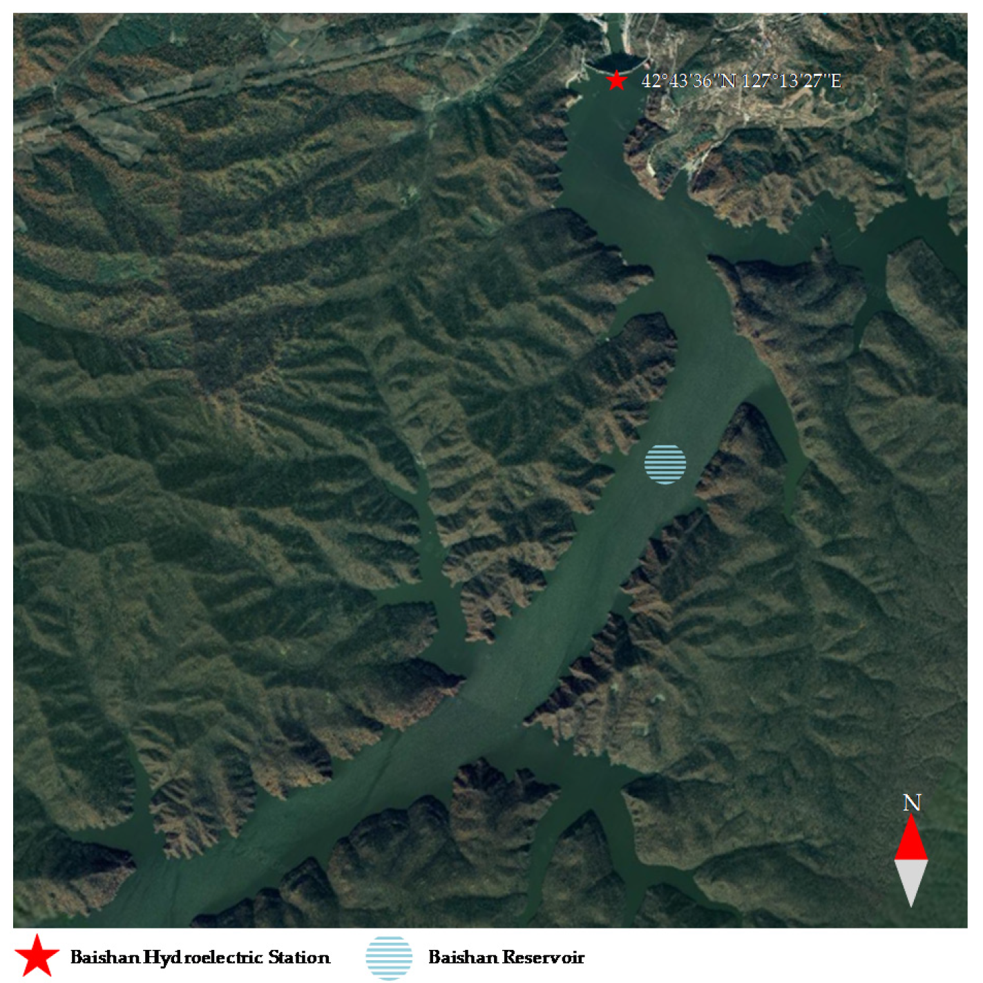
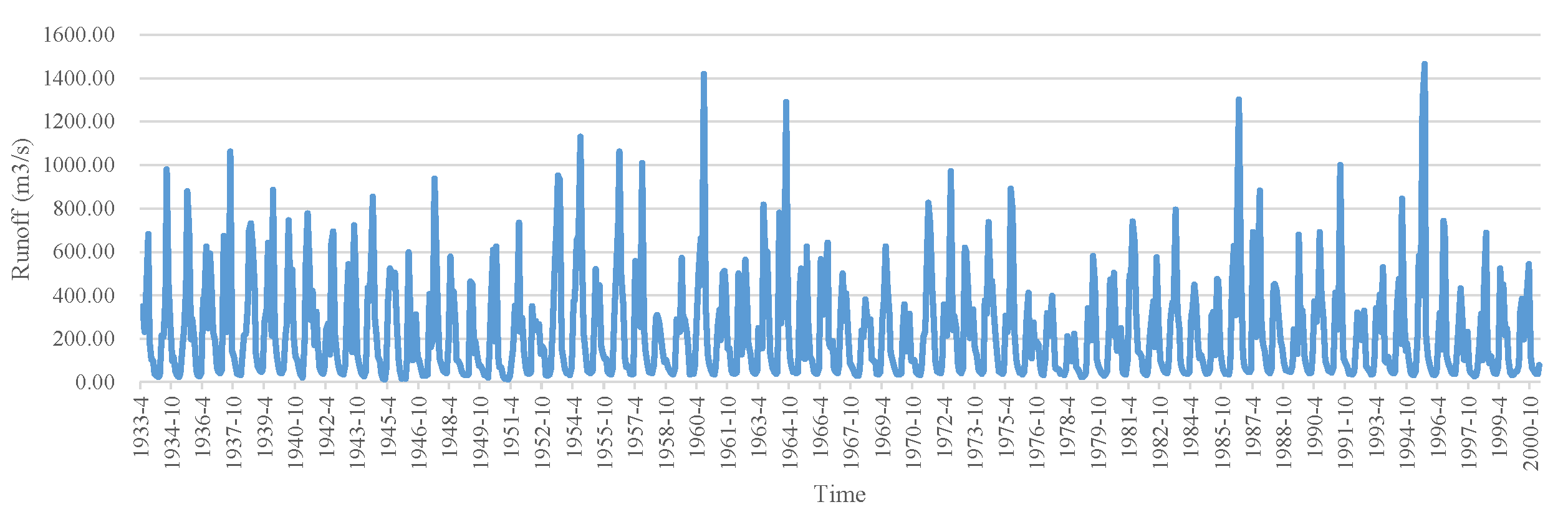
Baishan Hydropower Station in eastern Jilin Province of China has an installed capacity of approximately 1.5 GW and a storage capacity of 6.51 billion cubic meters, which plays a vital role in peak shaving and frequency regulation of the power system, as well as flood control during the flood period. The location of Baishan Hydropower Station is depicted in Figure 4. Moreover, the Baishan reservoir, located in the upstream of the Second Songhua River, has possessed incomplete regulation performance for many years, where the annual average runoff amount is 228 m³/s. Hence, it is necessary to construct an accurate monthly runoff forecasting approach to achieve better dispatching effectiveness for the reservoir. Additionally, the annual dispatching cycle of Baishan reservoir is generally from April of the current year to March of the next year. For this purpose, the monthly runoff series collected from April 1933 to March 2001 is employed to evaluate the performance of the proposed method in this study, of which the collected dataset contains 816 samples and is illustrated in Figure 5. Meanwhile, the statistical information of the runoff data, such as mean value, maximum value, minimum value, and standard deviation value, is presented in

Table 1. Statistical information of the collected runoff series.

Datasets	Mean (m3/s)	Max. (m3/s)	Min. (m3/s)	Std.
Baishan	229.98	1466.00	12.60	232.08

. It can be seen from Figure 5 and Table 1 that the collected runoff series possesses intense nonlinearity and volatility, which may pose challenges to implementing accurate runoff forecasting. Moreover, the runoff series is partitioned into the training set and the testing set based on the ratio of 4:1, where the first 653 months of the runoff data (April 1933–August 1987) are employed for training and the remaining 163 months of the data (September 1987–March 2001) are selected to verify the developed model.

4.2. Experimental Description

To adequately assess the forecasting performance of the proposed compound approach, seven relevant models, including SVR, back propagation neural network (BPNN), CNN, GRU, CNNGRU, EMD–CNNGRU, CEEMDAN–CNNGRU, and TVFEMD–CNNGRU, were applied as comparison experiments, among which EMD and CEEMDAN were successively combined with CNNGRU to verify the superiority in terms of decomposition performance for the employed TVFEMD. Additionally, TVFEMD–CNNGRU was constructed based on TVFEMD and CNNGRU to test the effectiveness of the SE-based subseries recombination employed in the proposed model. Furthermore, it is worth noting that the data preprocessing approaches, including EMD, CEEMDAN, TVFEMD, and SE-based subseries recombination, were implemented with MATLAB (Mathematical computing software, Natick, Massachusetts, USA). In addition, the forecasting modules, including SVR, BPNN, CNN, GRU, and CNNGRU, were developed with Python, where the optimizer Adam was employed to optimize the basic parameters of the neural networks. Furthermore, for the approaches mentioned above, the corresponding inherent parameter settings are illustrated in

Table 2. Parameter setting for all the methods.

Models	Parameter	Setting Values
SE	Tolerance	0.2 times the standard deviation of the series
	Scale factor	1
	Vector dimension	3
CEEMDAN	Standard deviation of the added white noise	0.05
	Number of realizations	500
	The allowed maximum number of sifting iterations	5000
TVF-EMD	B-spline order n	26
	Bandwidth threshold ξ	0.2
SVR	Regularization coefficient c	[2−10, 210]
	Kernel parameter g	[2−10, 210]
BPNN	Number of hidden layer nodes	32
	Number of hidden layers	1
	Size of batch	128
	Epochs of training	500
	Activation function	hyperbolic tangent (tanh)
CNN	Number of kernels	32
	Size of max-pooling	2
	Kernel size	3
	Size of batch	128
	Epochs of training	500
	Activation function	ReLU
GRU	Number of hidden layer nodes	32
	Number of hidden layers	1
	Size of batch	128
	Epochs of training	500
	Activation function	tanh
CNNGRU	Number of kernels	3
	Kernel size	16
	Size of max-pooling	2
	Number of hidden layer nodes	32
	Number of hidden layers	1
	Size of batch	128
	Epochs of training	500
	Activation function	RuLU (CNN)/tanh (GRU)

, among which the parameters of SVR were determined by grid search, and the hyperparameters within all the deep networks were obtained by the trial and error approach [38].

Subsequently, the collected runoff series was decomposed into several sets of subsequences by adopting EMD, CEEMDAN, TVFEMD, and TVFEMD combined with subseries recombination with the parameters expressed in Table 2, where the processed subseries are depicted in Figure 6. Based on the comparisons among Figure 6a–c, it can be found that modal-aliasing can be observed from the subseries decomposed by EMD and CEEMDAN, while such a phenomenon can be effectively handled by TVFEMD. Furthermore, it can be seen from Figure 6c,d that the number of subseries is significantly decreased by incorporating the SE-based subseries recombination into TVFEMD, which contributes to further reducing the time computation of the proposed model.

Furthermore, four commonly employed indicators, namely, root-mean-square error (RMSE), mean absolute error (MAE), mean absolute percentage error (MAPE), correlation coefficient (R²), and the Nash–Sutcliffe efficiency coefficient (CE), were adopted to quantitatively evaluate all the experimental models, which can contribute scientifically to interpreting the improvements obtained by the proposed approach [39]. They are illustrated in

Table 3. Evaluation metrics of the root-mean-square error (RMSE), the mean absolute error (MAE), the mean absolute percentage error (MAPE), and the correlation coefficient (R²).

Indicators	Explanation	Representation
RMSE	Root-mean-square error (m3/s)	$RMSE=\sqrt{\frac{1}{N}{\displaystyle \sum }_{i=1}^N{(Y_i-{\widehat{Y}}_i)}^2}$
MAE	Mean absolute error (m3/s)	$MAE=\frac{1}{N}{\displaystyle {\displaystyle \sum }_{i=1}^N}\left|Y_i-{\widehat{Y}}_i\right|$
MAPE	Absolute percentage error (%)	$MAPE=\frac{1}{N}{\displaystyle {\displaystyle \sum }_{i=1}^N}\left|\frac{100\times \left(Y_i-{\widehat{Y}}_i\right)}{Y_i}\right|$
R2	Correlation coefficient	$R^2=\frac{{\left(N{{\displaystyle \sum }}_{i=1}^N{\widehat{Y}}_i{Y}_i-{{\displaystyle \sum }}_{i=1}^N{\widehat{Y}}_i{{\displaystyle \sum }}_{i=1}^N{Y}_i\right)}^2}{\left(N{{\displaystyle \sum }}_{i=1}^N{\widehat{Y}}_i^2-{\left({{\displaystyle \sum }}_{i=1}^N{\widehat{Y}}_i\right)}^2\right)\left(N{{\displaystyle \sum }}_{i=1}^N{Y}_i^2-{\left({{\displaystyle \sum }}_{i=1}^N{Y}_i\right)}^2\right)}$
CE	Nash–Sutcliffe efficiency coefficient	$CE=1-\frac{{{\displaystyle \sum }}_{i=1}^N{(Y_i-{\widehat{Y}}_i)}^2}{{{\displaystyle \sum }}_{i=1}^N{(Y_i-{\widehat{Y}}_i)}^2}$

.

Where Y and $\hat{Y}$ indicate the actual value and predicted value, $\overline{Y}$ is the mean value of the actual values, and N is the number of predicted series. Additionally, the decline rates of RMSE, MAE, and MAPE, as well as the Diebold-Mariano (DM) test [40], were employed to reveal the differences between the experimental models, where the definition of the decline ratios are demonstrated in

Table 4. Decline ratios of metrics RMSE, MAE, and MAPE.

Indicators	Explanation	Representation
$P_{\mathit{RMSE}}$	Decline ratio of RMSE	$P_{RMSE}=\left(\frac{RMS{E}_a-RMS{E}_b}{RMS{E}_a}\right)$
$P_{\mathit{MAE}}$	Decline ratio of MAE	$P_{MAE}=\left(\frac{MA{E}_a-MA{E}_b}{MA{E}_a}\right)$
$P_{\mathit{MAPE}}$	Decline ratio of MAPE	$P_{MAPE}=\left(\frac{MAP{E}_a-MAP{E}_b}{MAP{E}_a}\right)$

. Moreover, for the given confidence level α, the critical difference in terms of forecasting performance obtained between the proposed approach and the contrastive ones can be claimed as less, applying the null hypothesis H₀. In contrast, H₁ possesses the opposite meaning of H₀. Hence, for the predicted errors obtained by all the models, the definition of the DM test is exhibited as follows:

$$DM=\frac{\frac{1}{N}{{\displaystyle \sum }}_{i=1}^N\left(L\left(erro{r}_i^1\right)-L\left(erro{r}_i^2\right)\right)}{\sqrt{s^2/N}}{s}^2$$

(5)

where s² denotes the estimation for the variance of ${L(\mathrm{error}}_i^1{) - L(\mathrm{error}}_i^2)$. Subsequently, in the light of the relationship between the calculated DM value and Z_α/2, the hypotheses mentioned above can be determined.

4.3. Contrastive Analyses

In this section, the quantitative evaluations for all the forecasting approaches will be analyzed and discussed, among which evaluation indicators RMSE, MAE, MAPE, R² and CE, obtained by all the experimental models, are exhibited in

Table 5. Evaluation metrics of all the experimental models.

Models	RMSE (m3/s)	MAE (m3/s)	MAPE (%)	R2	CE
SVR	174.2332	118.1611	0.9999	0.6488	0.4069
BPNN	173.3733	119.4081	0.9974	0.6539	0.4127
CNN	168.8239	114.2668	0.9054	0.6748	0.4431
GRU	169.8721	110.8002	0.8497	0.6674	0.4362
CNNGRU	167.3551	108.9287	0.7550	0.6752	0.4528
EMD-CNNGRU	145.9209	113.1712	1.0718	0.7665	0.5840
CEEMDAN-CNNGRU	129.8612	98.5647	0.9257	0.8241	0.6705
TVFEMD-CNNGRU	67.7378	51.5727	0.5395	0.9544	0.9104
TVFEMD-SE-CNNGRU	65.6926	52.1495	0.5697	0.9633	0.9157

, where the metrics obtained by the proposed model are marked in boldface. Moreover, the corresponding decline ratios of RMSE, MAE, and MAPE, calculated between the proposed model and the contrast ones, are demonstrated in

Table 6. Indicator decline ratios and the Diebold–Mariano (DM) test results illustrating the performance improvement of the proposed model.

Models	PRMSE (%)	PMAE (%)	PMAPE (%)	DM test
SVR	61.12	56.35	46.04	3.5571 ***
BPNN	60.93	56.81	45.90	4.0079 ***
CNN	59.88	54.87	40.41	3.8229 ***
GRU	60.12	53.45	36.50	3.6708 ***
CNNGRU	59.52	52.65	28.54	3.8433 ***
EMD-CNNGRU	53.58	54.43	49.66	4.6821 ***
CEEMDAN-CNNGRU	47.84	47.68	41.72	4.3568 ***
TVFEMD-CNNGRU	3.02	−1.12	−5.59	0.5830

*** is the 1% significance level.

. The results of the DM test for all the contrastive models are also illustrated in Table 6. Following the sufficient evaluation metrics presented in Table 5 and Table 6, several hypotheses and conclusions can be drawn as follows:

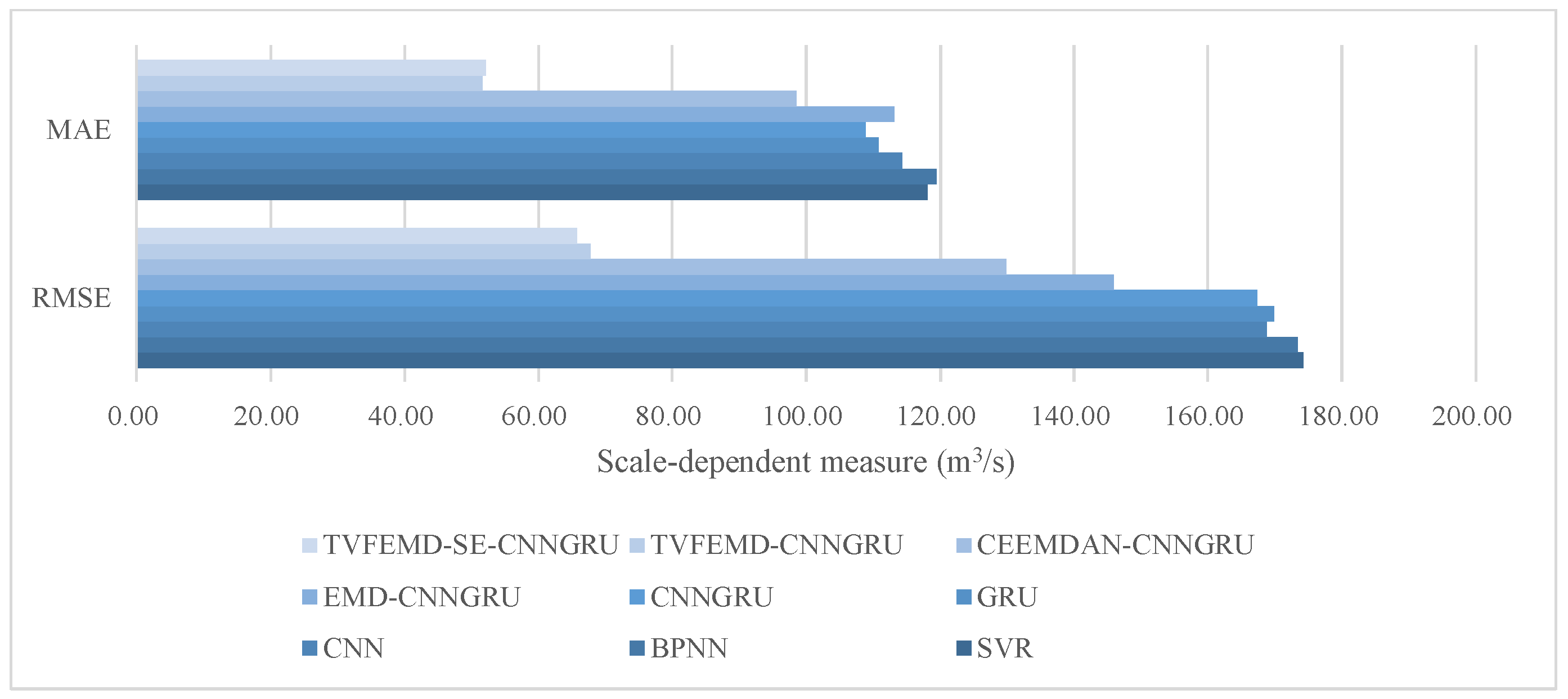
• Focusing on the comparisons among SVR, BPNN, CNN, GRU, and CNNGRU, it can be observed that the newly developed CNNGRU achieves the minimum indicator values in terms of RMSE, MAE, and MAPE as 167.3551, 108.9287 and 0.7550, while the corresponding correlation coefficient R² of CNNGRU is the maximum at 0.6752. Hence, it can be affirmed that preferable forecasting performance can be obtained by the newly constructed CNNGRU. However, compared to the remaining single models, the average decline ratios of RMSE, MAE, and MAPE, obtained by CNNGRU, are 2.44%, 5.74%, and 19.13%, respectively. Similarly, the metric CE obtained by CNNGRU is 0.4528, which achieves an average improvement of 6.14% compared with the remaining single models, thus indicating that the performance gaps among the single models are not significant. A reasonable hypothesis to interpret the phenomenon could be inferred, namely, that the forecasting capability of the aforementioned individual models would be significantly restricted by the volatility of the runoff series.
• Further contrasting the evaluation results obtained by CNNGRU, EMD-CNNGRU, CEEMDAN-CNNGRU, and TVFEMD-CNNGRU, it can be found that the forecasting accuracy can be markedly enhanced by adopting the decomposition techniques, except for EMD. Specifically, compared with EMD-CNNGRU, the CEEMDAN-based model possesses better forecasting performance in terms of RMSE, MAE, and MAPE, where the corresponding decline rates are 11.01%, 12.91%, and 13.63%, respectively. Additionally, the indicators RMSE, MAE, and MAPE of TVFEMD-CNNGRU are 67.7378, 51.5727, and 0.5395, which are the minimum values, and achieve the averaged descents of 53.65%, 51.59%, and 39.97% compared with CNNGRU, EMD-CNNGRU, and CEEMDAN-CNNGRU. It can be found that the TVFEMD-based model estimates more significant index decline rates, which can be attributed to the fact that the modal-aliasing existing in EMD and CEEMDAN can be effectively handled by TVFEMD, thus completing the superior decomposition performance.
• On the basis of TVFEMD-CNNGRU, the SE-based subseries recombination is introduced in the proposed model, with which the number of decomposed subsequences can be significantly reduced. The metrics of RMSE, MAE, and MAPE, obtained by the proposed model, are 65.6926, 52.1495, and 0.5697, which are close to the metrics obtained by TVFEMD-CNNGRU. It can be observed that the metrics MAE and MAPE of the proposed model are slightly more extensive than those of TVFEMD-CNNGRU, while the metrics R² and CE of the proposed model is the maximum among all the models at 0.9633 and 0.9157. Additionally, considering the same networks applied for the preprocessed subseries in both TVFEMD-based models, the proposed model, adopting the SE-based subseries recombination, possesses fewer subseries to be predicted, thus achieving less computational complexity compared with TVFEMD-CNNGRU. Furthermore, it can be observed from the results of the DM test illustrated in Table 6 that all the values are larger than 2.5800, which practically corresponds to the critical value of significance level 1%, except for TVFEMD-CNNGRU, with which it can be concluded that the proposed model achieves a significant promotion in forecasting accuracy, as well as a reduction of the computational cost, without significantly reducing prediction accuracy when compared with TVFEMD-CNNGRU.

On the other hand, the fitting curves obtained by single models and the combined ones are exhibited in Figure 7 and Figure 8, respectively, where the actual values are represented in the blue histogram for better distinction from the predicted and the actual values. It can be observed from Figure 7 that the fitting curve of CNNGRU is closer to the actual values, and achieves better performance at the peaks, while satisfactory forecasting results cannot be obtained by the single models. In contrast, as illustrated in Figure 8, it can be found that the combined models, applying decomposition approaches, possess fitting curves that are closer to the actual values.

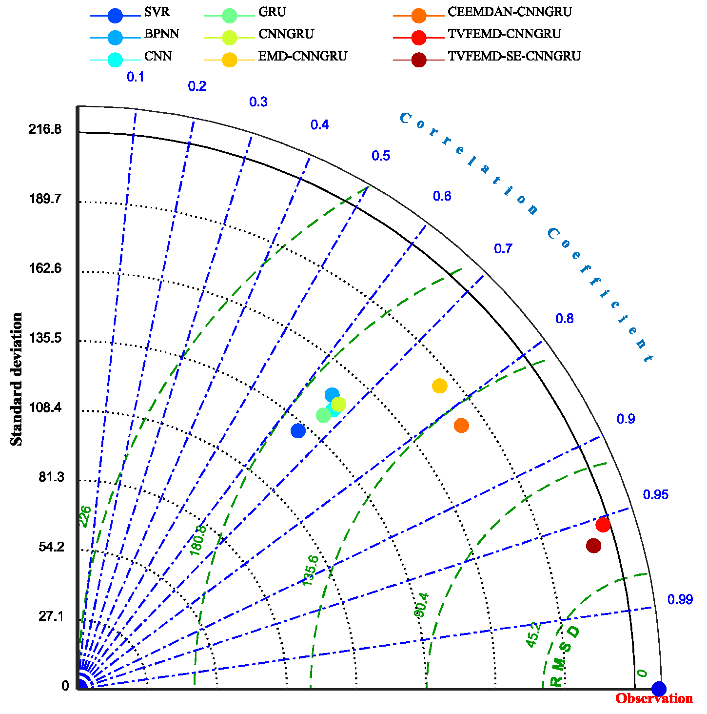
Additionally, the bar diagrams for RMSE, MAE, MAPE, and R² are expressed in Figure 9, Figure 10 and Figure 11 in order to visually observe the fluctuation trends of the metrics obtained by the various models, from which it can be seen that the conclusion claimed above can be drawn out intuitively. The combined model, based on decomposition approaches, can obtain much better forecasting results, while the TVFEMD-based models are superior to all the models. Moreover, the proposed model, applying TVFEMD, subseries recombination, and CNNGRU, achieves a significant reduction in computational resources without a significant decrease in forecasting accuracy. In addition, the Taylor diagram, which demonstrates the performance of the forecasting models in terms of the correlation coefficient, centered root mean square difference (RMSD), and standard deviation visually [26], is depicted in Figure 12. As shown in Figure 12, the proposed model, represented by the brown dot, is closer to the observation in the light of the above three indicators. Furthermore, based on the visualization of all the metric decline ratios presented in Figure 13, the metrics of the proposed model are generally (more than 40%) decreased compared with all the other models except TVFEMD-CNNGRU, thus intuitively testifying to Conclusion (3) discussed above.

5. Conclusions

To implement runoff forecasting with an improved balance between accuracy and efficiency, a novel composite approach coupling TVFEMD, subseries recombination based on SE, and the newly constructed deep network CNNGRU is proposed in this study. Among the methods, TVFEMD was applied to decompose the collected runoff series into a set of subsequences, thus weakening the volatility of the runoff series. The initially decomposed subsequences were recombined according to the SE values of all the subseries and the recombination criterion. Subsequently, CNNGRU was adopted to obtain the prediction values of all the preprocessed subseries, after which the final forecasting results were deduced by the accumulation of the prediction results obtained above. Additionally, eight relevant contrastive models were applied to the runoff series collected from the Baishan reservoir, where the experimental results demonstrated that (1) TVFEMD possesses superior decomposition performance compared with EMD and CEEMDAN. Thus, the TVFEMD-based combined models achieved satisfactory forecasting results. (2) The SE-based subseries recombination is conducive to reducing the time computation of the whole model without significantly decreasing prediction accuracy. (3) The newly developed deep network, namely, CNNGRU, can capture the intrinsic characteristics within runoff series commendably, thus obtaining satisfactory estimation results. In summary, the proposed compound runoff forecasting approach, which balances prediction accuracy and computational efficiency, can be applied as a potent tool to implement better water resource management.

References

- Feng, Z.; Niu, W.; Zhou, J.; Cheng, C. Linking Nelder-Mead Simplex Direct Search Method into Two-Stage Progressive Optimality Algorithm for Optimal Operation of Cascade Hydropower Reservoirs. J. Water Resour. Plan. Manag. 2020, 146, 4020019. [Google Scholar] [CrossRef]
- Feng, Z.-K.; Niu, W.-J.; Tang, Z.-Y.; Jiang, Z.-Q.; Xu, Y.; Liu, Y.; Zhang, H. Monthly runoff time series prediction by variational mode decomposition and support vector machine based on quantum-behaved particle swarm optimization. J. Hydrol. 2020, 583, 124627. [Google Scholar] [CrossRef]
- He, X.; Luo, J.; Li, P.; Zuo, G.; Xie, J. A Hybrid Model Based on Variational Mode Decomposition and Gradient Boosting Regression Tree for Monthly Runoff Forecasting. Water Resour. Manag. 2020, 34, 865–884. [Google Scholar] [CrossRef]
- Chang, F.J.; Guo, S. Advances in hydrologic forecasts and water resources management. Water 2020, 12, 1819. [Google Scholar] [CrossRef]
- Zounemat-Kermani, M.; Matta, E.; Cominola, A.; Xia, X.; Zhang, Q.; Liang, Q.; Hinkelmann, R. Neurocomputing in Surface Water Hydrology and Hydraulics: A Review of Two Decades Retrospective, Current Status and Future Prospects. J. Hydrol. 2020, 125085. [Google Scholar] [CrossRef]
- Peng, T.; Zhou, J.; Zhang, C.; Fu, W. Streamflow forecasting using empirical wavelet transform and artificial neural networks. Water 2017, 9, 406. [Google Scholar] [CrossRef] [Green Version]
- Zhou, J.; Peng, T.; Zhang, C.; Sun, N. Data pre-analysis and ensemble of various artificial neural networks for monthly streamflow forecasting. Water 2018, 10, 628. [Google Scholar] [CrossRef] [Green Version]
- Napolitano, G.; Serinaldi, F.; See, L. Impact of EMD decomposition and random initialisation of weights in ANN hindcasting of daily stream flow series: An empirical examination. J. Hydrol. 2011, 406, 199–214. [Google Scholar] [CrossRef]
- Sun, Y.; Niu, J.; Sivakumar, B. A comparative study of models for short-term streamflow forecasting with emphasis on wavelet-based approach. Stoch. Environ. Res. Risk Assess. 2019, 33, 1875–1891. [Google Scholar] [CrossRef]
- Huang, S.; Chang, J.; Huang, Q.; Chen, Y. Monthly streamflow prediction using modified EMD-based support vector machine. J. Hydrol. 2014, 511, 764–775. [Google Scholar] [CrossRef]
- Parviz, L.; Rasouli, K. Development of Precipitation Forecast Model Based on Artificial Intelligence and Subseasonal Clustering. J. Hydrol. Eng. 2019, 24, 1–13. [Google Scholar] [CrossRef]
- Kimura, N.; Yoshinaga, I.; Sekijima, K.; Azechi, I.; Baba, D. Convolutional neural network coupled with a transfer-learning approach for time-series flood predictions. Water 2020, 12, 96. [Google Scholar] [CrossRef] [Green Version]
- Chang, L.C.; Chang, F.J.; Yang, S.N.; Kao, I.F.; Ku, Y.Y.; Kuo, C.L.; Amin, I.M.Z.b.M. Building an intelligent hydroinformatics integration platform for regional flood inundation warning systems. Water 2018, 11, 9. [Google Scholar] [CrossRef] [Green Version]
- Lee, D.; Lee, G.; Kim, S.; Jung, S. Future Runoff Analysis in the Mekong River Basin under a Climate Change Scenario Using Deep Learning. Water 2020, 12, 1556. [Google Scholar] [CrossRef]
- Gao, S.; Huang, Y.; Zhang, S.; Han, J.; Wang, G.; Zhang, M.; Lin, Q. Short-term runoff prediction with GRU and LSTM networks without requiring time step optimization during sample generation. J. Hydrol. 2020, 589, 125188. [Google Scholar] [CrossRef]
- Bojang, P.O.; Yang, T.C.; Pham, Q.B.; Yu, P.S. Linking singular spectrum analysis and machine learning for monthly rainfall forecasting. Appl. Sci. 2020, 10, 3224. [Google Scholar] [CrossRef]
- Zhou, T.; Wang, F.; Yang, Z. Comparative analysis of ANN and SVM models combined with wavelet preprocess for groundwater depth prediction. Water 2017, 9, 781. [Google Scholar] [CrossRef] [Green Version]
- Kao, I.-F.; Zhou, Y.; Chang, L.-C.; Chang, F.-J. Exploring a Long Short-Term Memory based Encoder-Decoder framework for multi-step-ahead flood forecasting. J. Hydrol. 2020, 583, 124631. [Google Scholar] [CrossRef]
- Hochreiter, S.; Schmidhuber, J. Long Short-Term Memory. Neural Comput. 1997, 9, 1735–1780. [Google Scholar] [CrossRef]
- Cho, K.; Van Merriënboer, B.; Gulcehre, C.; Bahdanau, D.; Bougares, F.; Schwenk, H.; Bengio, Y. Learning phrase representations using RNN encoder-decoder for statistical machine translation. In Proceedings of the 2014 Conference on Empirical Methods in Natural Language Processing, EMNLP, Doha, Qatar, 26–28 October 2014; pp. 1724–1734. [Google Scholar]
- Apaydin, H.; Feizi, H.; Sattari, M.T.; Colak, M.S.; Shamshirband, S.; Chau, K.W. Comparative analysis of recurrent neural network architectures for reservoir inflow forecasting. Water 2020, 12, 1500. [Google Scholar] [CrossRef]
- Liu, H.; Mi, X.; Li, Y.; Duan, Z.; Xu, Y. Smart wind speed deep learning based multi-step forecasting model using singular spectrum analysis, convolutional Gated Recurrent Unit network and Support Vector Regression. Renew. Energy 2019, 143, 842–854. [Google Scholar] [CrossRef]
- Tan, Q.F.; Lei, X.H.; Wang, X.; Wang, H.; Wen, X.; Ji, Y.; Kang, A.Q. An adaptive middle and long-term runoff forecast model using EEMD-ANN hybrid approach. J. Hydrol. 2018, 567, 767–780. [Google Scholar] [CrossRef]
- Yang, W.; Wang, J.; Lu, H.; Niu, T.; Du, P. Hybrid wind energy forecasting and analysis system based on divide and conquer scheme: A case study in China. J. Clean. Prod. 2019, 222, 942–959. [Google Scholar] [CrossRef] [Green Version]
- Colominas, M.A.; Schlotthauer, G.; Torres, M.E. Improved complete ensemble EMD: A suitable tool for biomedical signal processing. Biomed. Signal Process. Control 2014, 14, 19–29. [Google Scholar] [CrossRef]
- Wen, X.; Feng, Q.; Deo, R.C.; Wu, M.; Yin, Z.; Yang, L.; Singh, V.P. Two-phase extreme learning machines integrated with the complete ensemble empirical mode decomposition with adaptive noise algorithm for multi-scale runoff prediction problems. J. Hydrol. 2019, 570, 167–184. [Google Scholar] [CrossRef]
- Li, H.; Li, Z.; Mo, W. A time varying filter approach for empirical mode decomposition. Signal Process. 2017, 138, 146–158. [Google Scholar] [CrossRef]
- Zhang, Y.; Liu, K.; Qin, L.; An, X. Deterministic and probabilistic interval prediction for short-term wind power generation based on variational mode decomposition and machine learning methods. Energy Convers. Manag. 2016, 112, 208–219. [Google Scholar] [CrossRef]
- Wang, J.; Li, Y. Multi-step ahead wind speed prediction based on optimal feature extraction, long short term memory neural network and error correction strategy. Appl. Energy 2018, 230, 429–443. [Google Scholar] [CrossRef]
- Jiang, Y.; Huang, G.; Yang, Q.; Yan, Z.; Zhang, C. A novel probabilistic wind speed prediction approach using real time refined variational model decomposition and conditional kernel density estimation. Energy Convers. Manag. 2019, 185, 758–773. [Google Scholar] [CrossRef]
- Zhou, K.-B.; Zhang, J.-Y.; Shan, Y.; Ge, M.-F.; Ge, Z.-Y.; Cao, G.-N. A Hybrid Multi-Objective Optimization Model for Vibration Tendency Prediction of Hydropower Generators. Sensors 2019, 19, 2055. [Google Scholar] [CrossRef] [Green Version]
- Sun, W.; Wang, Y. Short-term wind speed forecasting based on fast ensemble empirical mode decomposition, phase space reconstruction, sample entropy and improved back-propagation neural network. Energy Convers. Manag. 2018, 157, 1–12. [Google Scholar] [CrossRef]
- Ding, L.; Fang, W.; Luo, H.; Love, P.E.D.; Zhong, B.; Ouyang, X. A deep hybrid learning model to detect unsafe behavior: Integrating convolution neural networks and long short-term memory. Autom. Constr. 2018, 86, 118–124. [Google Scholar] [CrossRef]
- Mi, X.; Liu, H.; Li, Y. Wind speed prediction model using singular spectrum analysis, empirical mode decomposition and convolutional support vector machine. Energy Convers. Manag. 2019, 180, 196–205. [Google Scholar] [CrossRef]
- Chai, J.; Wang, Y.; Wang, S.; Wang, Y. A decomposition–integration model with dynamic fuzzy reconstruction for crude oil price prediction and the implications for sustainable development. J. Clean. Prod. 2019, 229, 775–786. [Google Scholar] [CrossRef]
- Zheng, W.; Peng, X.; Lu, D.; Zhang, D.; Liu, Y.; Lin, Z.; Lin, L. Composite quantile regression extreme learning machine with feature selection for short-term wind speed forecasting: A new approach. Energy Convers. Manag. 2017, 151, 737–752. [Google Scholar] [CrossRef]
- Wang, C.; Zhang, H.; Fan, W.; Ma, P. A new chaotic time series hybrid prediction method of wind power based on EEMD-SE and full-parameters continued fraction. Energy 2017, 138, 977–990. [Google Scholar] [CrossRef]
- Gemperline, P.J.; Long, J.R.; Gregoriou, V.G. Nonlinear multivariate calibration using principal components regression and artificial neural networks. Anal. Chem. 1991, 63, 2313–2323. [Google Scholar] [CrossRef]
- Hyndman, R.J.; Koehler, A.B. Another look at measures of forecast accuracy. Int. J. Forecast. 2006, 22, 679–688. [Google Scholar] [CrossRef] [Green Version]
- Diebold, F.X.; Mariano, R.S. Comparing predictive accuracy. J. Bus. Econ. Stat. 2002, 20, 134–144. [Google Scholar] [CrossRef]
Figure 1.
The structure of the gated recurrent unit network (GRU).
Figure 2.
The structure of the convolutional neural network incorporated into GRU with deep sequential structure (CNNGRU).
Figure 3.
The flow chart of the proposed compound approach.
Figure 4.
Location of Baishan Hydropower Station.
Figure 5.
Runoff series collected from Baishan Hydropower Station.
Figure 6.
The decomposed subsequences are obtained by applying (a) empirical mode decomposition (EMD), (b) complete ensemble EMD with adaptive noise (CEEMDAN), (c) time-varying filter into the shifting process of EMD (TVFEMD), and (d) TVFEMD combined with sample entropy (SE)-based subseries recombination.
Figure 7.
Forecasting curves estimated by all the single models.
Figure 8.
Forecasting curves estimated by a novel deep sequential structure incorporating CNN into GRU (CNNGRU) and all the decomposition-based models.
Figure 9.
Histogram of metrics MAE and RMSE.
Figure 10.
Histogram of metric MAPE.
Figure 11.
Histogram of metrics MAE and R2.
Figure 12.
Taylor diagram for the visualized evaluation for all the models.
Figure 13.
Visualization of all the metric decline ratios.