An Accelerated Tool for Flood Modelling Based on Iber
by
 , , and
Orlando García-Feal
1,* ,
,
José González-Cao
1,
Moncho Gómez-Gesteira
1, 
Luis Cea
2,
José Manuel Domínguez
1 and
Arno Formella
3 1
Environmental Physics Laboratory (EPHYSLAB), Universidad de Vigo, Campus As Lagoas s/n, 32004 Ourense, Spain
2
Environmental and Water Engineering Group, Departamento de Ingeniería Civil, Universidade da Coruña, Campus Elviña s/n, E-15071 A Coruña, Spain
3
Laboratorio de Informática Aplicada, Universidade de Vigo, Campus As Lagoas s/n, 32004 Ourense, Spain
*
Author to whom correspondence should be addressed.
Water 2018, 10(10), 1459; https://doi.org/10.3390/w10101459
Submission received: 27 September 2018
/
Revised: 11 October 2018
/
Accepted: 14 October 2018
/
Published: 16 October 2018
(This article belongs to the Special Issue Selected Papers from the 1st International Electronic Conference on the Hydrological Cycle (ChyCle-2017))
Abstract
:This paper presents Iber+, a new parallel code based on the numerical model Iber for two-dimensional (2D) flood inundation modelling. The new implementation, which is coded in C++ and takes advantage of the parallelization functionalities both on CPUs (central processing units) and GPUs (graphics processing units), was validated using different benchmark cases and compared, in terms of numerical output and computational efficiency, with other well-known hydraulic software packages. Depending on the complexity of the specific test case, the new parallel implementation can achieve speedups up to two orders of magnitude when compared with the standard version. The speedup is especially remarkable for the GPU parallelization that uses Nvidia CUDA (compute unified device architecture). The efficiency is as good as the one provided by some of the most popular hydraulic models. We also present the application of Iber+ to model an extreme flash flood that took place in the Spanish Pyrenees in October 2012. The new implementation was used to simulate 24 h of real time in roughly eight minutes of computing time, while the standard version needed more than 15 h. This huge improvement in computational efficiency opens up the possibility of using the code for real-time forecasting of flood events in early-warning systems, in order to help decision making under hazardous events that need a fast intervention to deploy countermeasures.
Keywords:
flood; numerical simulation; shallow water equations; Iber+; benchmark; CUDA; OpenMP; finite volume1. Introduction
Floods are a type of natural disaster that have affected human activity throughout history. In recent years, these phenomena have become more frequent and intense due to climate change [1,2]. The development of numerical tools that are able to simulate these events has become essential. These tools must be accurate, in order to provide useful data, as well as computationally efficient, to be able to obtain results in reasonable computational times. The information provided by the numerical models should help decision makers to design resilient structures, as well as to estimate the intensity of an imminent extreme event in order to implement countermeasures that avoid or mitigate the economic and human losses.
Iber [3] is a numerical model that solves the two-dimensional (2D) depth-averaged shallow water equations with an unstructured explicit finite volume solver. In addition to the hydraulic module, it has a sediment transport and a water quality module [4] to solve transport processes in free surface shallow flows. It implements the first order and second order extension of the upwind scheme of Roe [5] to model flood inundation, and the DHD (decoupled hydrological discretization) scheme [6] to solve the shallow water equations in rainfall–runoff applications. The algorithms implemented in the model have been extensively validated and applied in previous studies related to river inundation, tidal currents in estuaries and rainfall–runoff modelling [6,7,8,9,10].
One of the main limitations of Iber at the present time is the CPU time needed to perform simulations over complex and large spatial domains (of several km2). This is because the model lacks the necessary optimizations to take advantage of the parallelism available on current hardware. This hampers the use of the model in interesting applications such as real-time flood forecasting in early warning systems, Monte Carlo-based calibration and uncertainty analysis [10,11], high-resolution rainfall–runoff simulation in medium and large-size watersheds, or continuous simulation methods applied to flood frequency analysis [12].
Hydraulic models are commonly accelerated for shared memory multiprocessor systems with OpenMP (open multi-processing), but the speedup that can be achieved by this procedure is limited. Alternatively, MPI (message passing interface) can be used to take advantage of distributed memory supercomputers, but are expensive and difficult to maintain. Another way to accelerate this kind of code is the use of GPUs (graphical processing units). This technology offers a high amount of parallel processing power in quite inexpensive cards that can be installed in a server or workstation. GPUs have been employed successfully in mesh-free [13] and mesh-based [14,15,16,17] models reaching speedups of two orders of magnitude.
In this work, a new parallel implementation of the hydraulics module of Iber, named Iber+, is presented. The new code is written in C++ and it makes use of OpenMP and CUDA [18] to accelerate the simulations. The rest of this paper is organized as follows. In Section 2, the governing equations and the most relevant techniques used in the parallel implementation are detailed. In Section 3, four different benchmark cases are used to validate the accuracy and analyse the computational efficiency of Iber+ when compared with other hydraulic models. Finally, in Section 4, Iber+ is applied to compute rainfall–runoff during a real flash-flood event in a mountain headwater catchment of 240 km2.
2. Methods
2.1. Hydrodynamic Model
The 2D depth-averaged shallow water equations solved in Iber can be written as:
where h represents the water depth, and are the averaged horizontal velocities, is the acceleration of the gravity, is the density of the water, is the bed elevation, is the bed friction, is the turbulent viscosity, is the rainfall intensity and is the infiltration rate. Iber also implements terms to account for wind surface friction, the Coriolis acceleration and baroclinic pressure, but those terms are not included here for the sake of simplicity. In Iber, the bed friction is computed with the Manning formulation as:
2.2. Numerical Code Iber+
Iber+ is a new code that implements a parallelization of the hydraulic module of Iber [3], which is a hydraulic model that solves 2D shallow water equations using an unstructured finite volume solver. The software package Iber provides a user-friendly graphical user interface for pre- and post-processing and can be freely downloaded from http://iberaula.es. The Iber code is programmed in Fortran and it is partially parallelized with OpenMP. Even if the computation time is reduced by using this technique, the code is unable to efficiently use current multi-core processors, so the speedup that can be achieved is quite limited. Simulation time becomes critical when addressing certain kinds of problems such as real-time flood forecasting, Monte Carlo-based simulations, high-resolution rainfall–runoff modelling, or long term simulations.
The main aim of the Iber+ code is to significantly improve the computational efficiency of Iber, while being fully compatible with the Iber software. The new code has an object-oriented implementation programmed in C++. It is parallelized for shared memory systems with OpenMP and it also provides an Nvidia CUDA implementation for execution in GPUs.
OpenMP is an API (application programming interface) that allows easy parallelization of traditional loops using compiler directives. However, to achieve significant speedups, there are several aspects to be taken into account. The parallelization of a loop generates an overhead, so the parallelization of low-cycle loops could be counter-productive. It is also important to consider the granularity of loops. Combining simple loops into larger loops can reduce parallelism overhead, however this could affect the automatic vectorization. With vectorization enabled in the compiler, a program can use the SIMD (single instruction multiple data) instruction set, e.g., SSE (streaming SIMD extensions) or AVX (advanced vector extensions), that provides extra computing power in modern CPUs. However, loops that use branching or other complex structures may not be vectorized automatically. On the other hand, the principle of locality is fundamental. Modern CPUs have a complex memory hierarchy, including several levels of cache memory. Accessing a memory position that is not in cache implies a significant penalty. Therefore, memory access patterns should be studied and the design of suitable data structures is fundamental to achieve good performance. For instance, choices between using an array of structures or a structure of arrays should be evaluated for each algorithm.
GPUs use highly parallel architectures that confer them a high amount of computing power. This is needed to render complex 3D computer graphics scenes. Since most GPUs are programmable, the manufacturers provide APIs for GPGPU (general processing graphics processing unit) computing. This technology makes the processing power of GPUs available to problems not necessarily related to graphics. One of the most common GPGPU APIs used for scientific purposes is Nvidia CUDA, providing access to the GPUs with traditional programming languages like C/C++ or Fortran.
Nvidia GPUs are made of a large amount of processors organized in streaming multiprocessors (SMs) employing a single instruction multiple thread (SIMT) architecture. Each SM executes several threads in parallel, in groups of 32, called warps. All the threads start on the same program address but have their own registers. However, one warp can only execute one instruction at a time. If one of the threads branches to a different path than the rest, a divergence occurs. In that case, that path will be executed while the other threads are stalled, and later the other path, until the threads converge again. This procedure can produce a heavy performance penalty if it occurs frequently.
Another critical issue is reduction algorithms. In GPUs, global synchronization is expensive, so this kind of algorithm is not as trivial as in CPUs. To avoid heavy performance penalties, an alternative approach must be employed. In Iber+, the library Nvidia CUB (CUDA unbound) was employed to implement reduction algorithms. CUB is an open-source high performance library [19] developed by Nvidia that provides reusable pieces of software for CUDA programming.
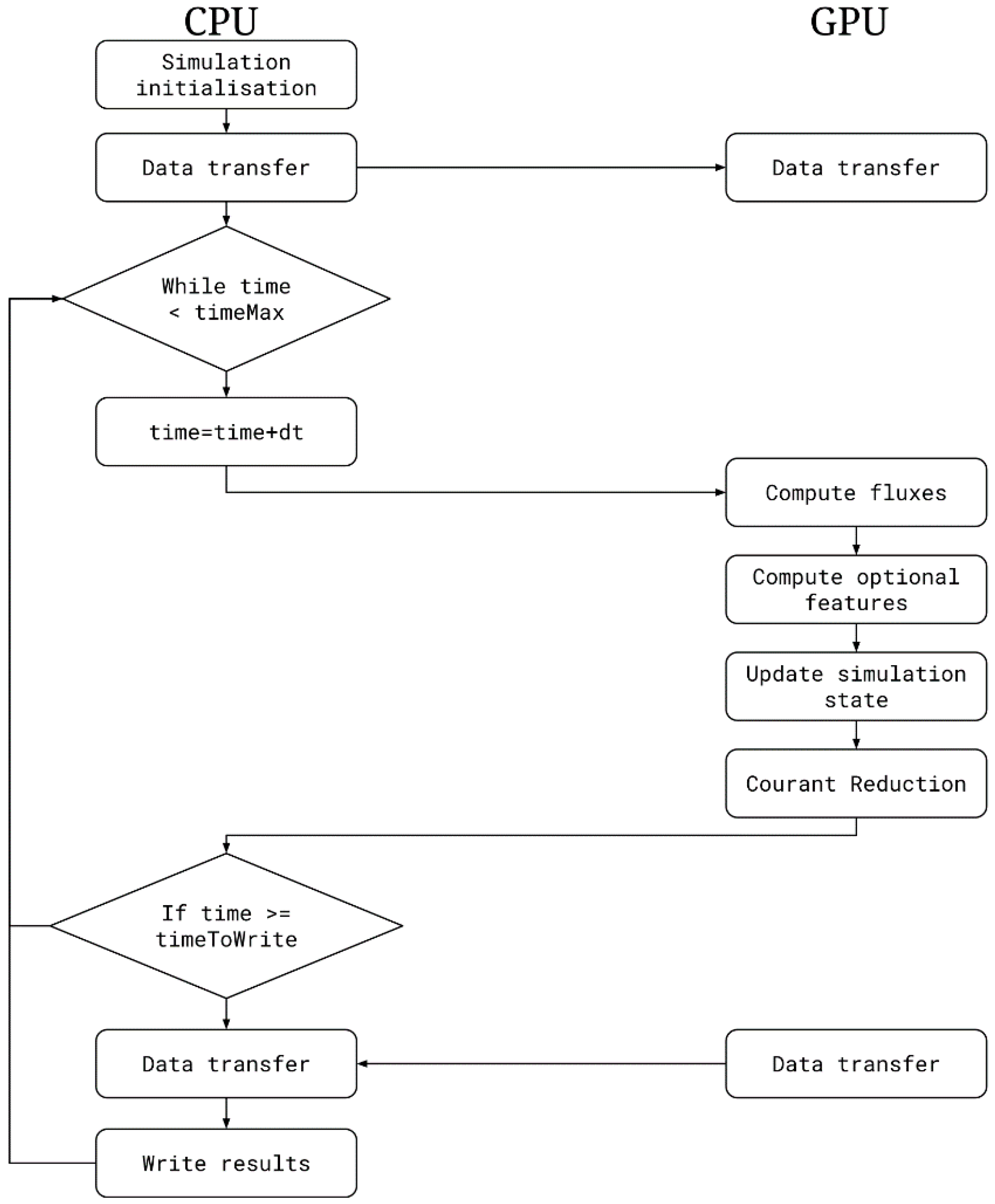
The last issue to address when programming GPUs is data transfer. Unlike integrated GPUs of mobile devices where the GPU and CPU share the same memory, discrete high-performance GPUs are issued in separate cards with their own memories. The GPU memory is usually faster and smaller than the main system memory and is located in a different address space. As the memory transfers from the system memory to the GPU memory are done via the PCI (peripheral component interconnect) bus, the bandwidth is limited and causes a bottleneck that needs attention. Even though the API can provide a unified address space, data transfers should be carefully made to avoid performance penalties. As data transfers are expensive, it could be more profitable to do certain computations (like reductions) on the GPU and being slower than on the CPU, rather than needing to transfer the data to system memory and run them on the CPU. Figure 1 shows the flow chart of the Iber+ execution. Once the simulation is started, most of the computations are performed on the GPU, minimizing the data transfers.
The speedup achieved by using a GPU in respect to the CPU implementation increases as the problem size gets bigger. The speedup increases until the GPU computation capacity is saturated; this occurs when all GPU processors are effectively used.
Both the Iber and Iber+ CPU code uses only double precision computations. However, in GPU computing, using double precision could suppose a considerable performance penalty. Depending on the specific GPU model, the theoretical performance in double precision could be from two to more than ten times slower [20]. In this work, the GPU computations were performed in single precision because no significant differences were found in the cases analyzed. However, some applications may require the use of double precision arithmetic, so this option will be added in further versions.
The Iber+ implementation is based on the Iber code, but reimplemented from scratch in C++. No substantial modifications were made to the original algorithms. The computations are made using unstructured meshes and the fluxes are solved at the edges of the underlying graph data structure. However, data structures were revised and optimized to reduce the memory footprint and to improve the memory access patterns. Even though Iber has most of its loops parallelized with OpenMP, these were redesigned in Iber+ to avoid critical regions and data dependencies that limited the speedup that could be achieved. These and other minor optimizations were done for the computation routines. Moreover, I/O (input/output) routines were optimized to avoid unnecessary data reading and writing.
For the GPU implementation, several drawbacks as mentioned previously should be considered. In order to achieve the highest speedup with GPU computing, memory transfers should be reduced as much as possible. Therefore, most of the computation routines were implemented in CUDA. Once the simulation is initialized, the data is transferred to the GPU. Then, most of the simulation is performed on the GPU and the only data transferred from the GPU are the results that should be written to disk or single variables like the time step. Additionally, as the CPU is free while the GPU is performing the computations, the CPU can run other tasks like writing the results to disk in parallel, hence, further improving the overall run time of the simulation.
3. Validation Tests
To validate the new code, four tests included in the benchmark of the hydraulic modelling packages published by the Environmental Agency of the U.K. government [21] were replicated. This benchmark consists of a set of nine tests that were run with 19 hydraulic models. The models were compared in terms of numerical accuracy and computational efficiency. Note that neither experimental nor theoretical solutions are provided as reference data, so the only way of comparing the model results is against other code. The three numerical models chosen to be compared with Iber and Iber+ are TUFLOW FV (v2012.000b) [22], InfoWorks ICM (v2.5.2) [23] and JFlow+ (v2.0) [14]. These models were chosen due their popularity [24] and similarity with Iber, since all of them solve 2D shallow water equations using finite volume solvers. Different hardware configurations were used in the validation of Iber+. The CPU simulations (both Iber and Iber+ CPU) were run in a server with an Intel Xeon E5-2695 v4 processor (18 cores). The GPU simulations (Iber+ GPU) were run in a workstation with an Intel Core i7-4770 CPU and two different GPUs: a modern GPU (Nvidia GTX 1080) and an older GPU (Nvidia GTX 480). The latter one was used to carry out a more objective comparison with JFlow+ and InfoWorks ICM, which used a Nvidia GTX 285 and a Nvidia Tesla C2050, respectively. The Nvidia GTX 480 offers a comparable performance [25,26] to those cards and shares the same architecture (Fermi) as the Tesla C2050. The main characteristics of the previously mentioned GPUs are shown in Table 1.
All the validation tests presented in this section were run with the first order of the discretization scheme of Roe and a wet-dry tolerance of 0.0001 m. Notice that the nomenclature of the tests, as well as the numbering of the control points, are the same as those used in [21] for an easier comparison with the original benchmark document.
3.1. Test 1: Flooding a Disconnected Water Body
3.1.1. Case Description
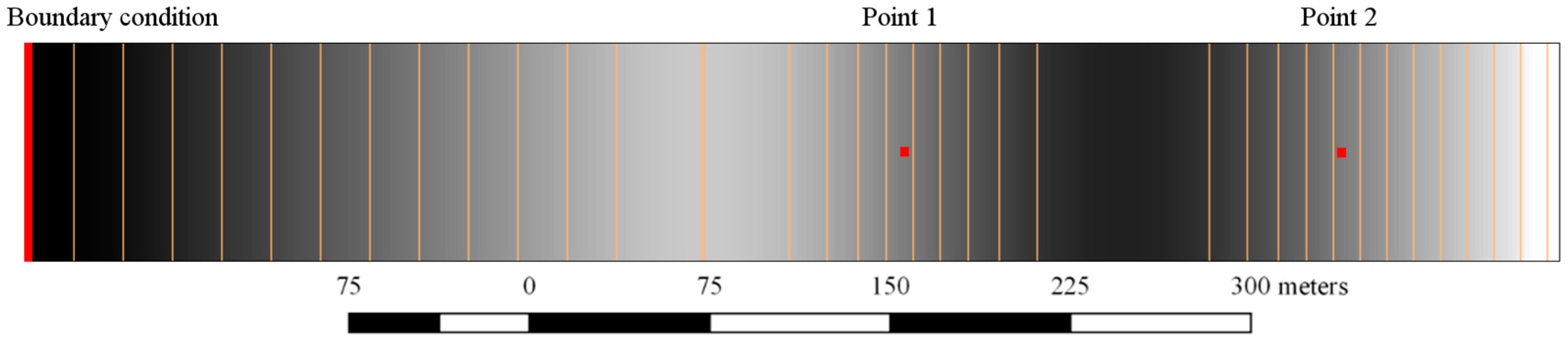
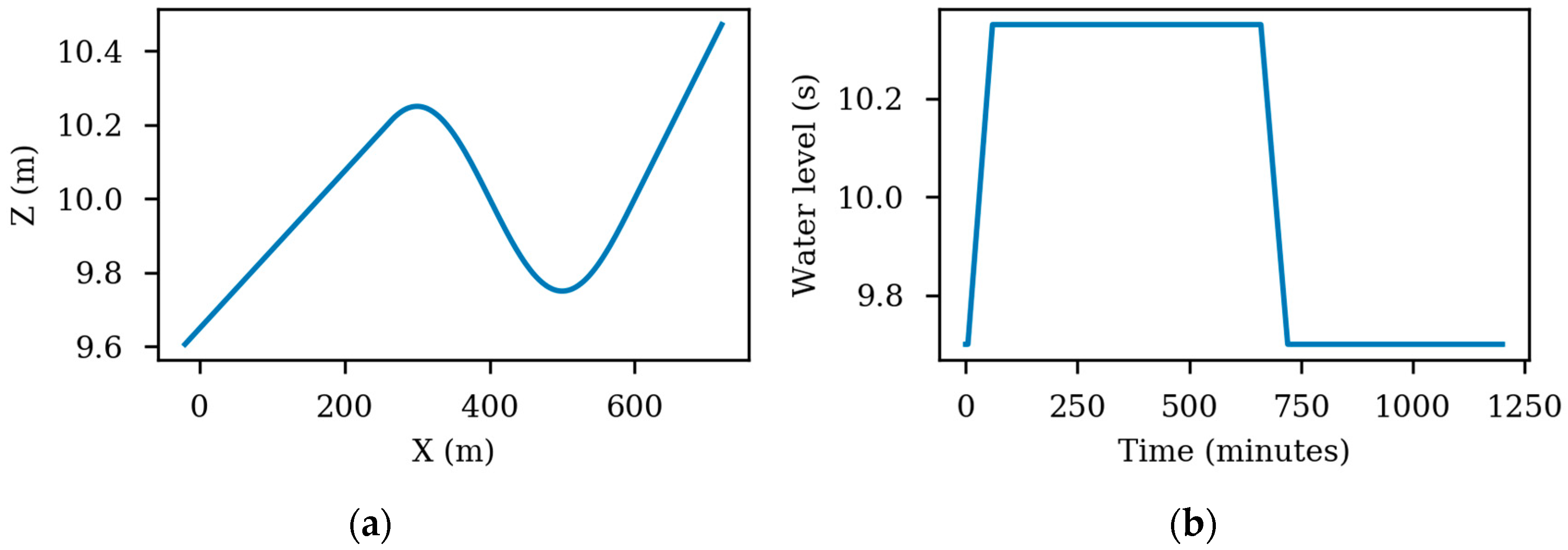
The first test is designed to check the basic capabilities of the hydraulic models. The domain is shown in Figure 2. It consists of a rectangular flume of 700 m length and 100 m width with a variable elevation (Figure 3a). The initial water level is 9.7 m in the whole flume. The spatial domain is discretized using a structured grid with an element size of 10 m. The Manning’s coefficient is set to 0.03 s/m1/3. The inlet boundary condition is defined at the left side of the domain (red line in Figure 2). The inlet hydrograph is shown in Figure 3b. The total physical time is 20 h. Time series of the water level were extracted at the two control points shown in Figure 2, in order to compare the results with the other software packages.
3.1.2. Results
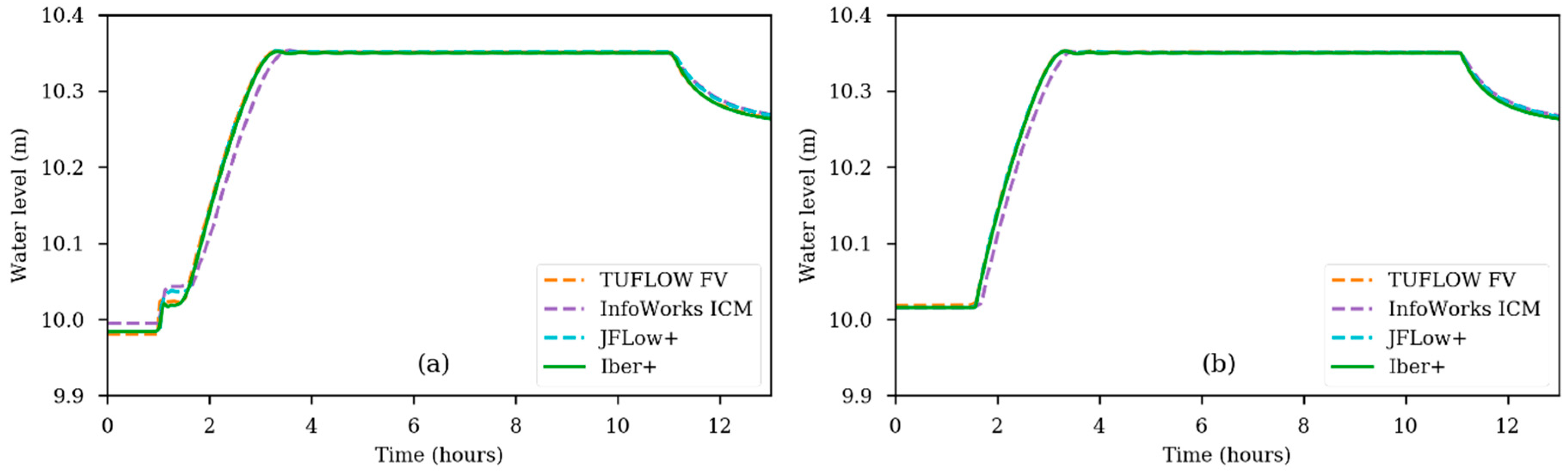
Figure 4 shows the time series of the water level obtained at the two control points for the simulations carried out with TUFLOW FV, InfoWorks ICM, JFlow+ and Iber+. The water levels obtained with Iber and Iber+ using both the CPU and GPU are almost the same. The differences are due to round-off errors of the different implementations. These differences could not be appreciated in the plots. The coefficient of variation of the RMSD (root mean square deviation) is defined as follows:
were x and y are the time series and N their number of elements. This was used to measure the error of Iber+ (including CPU and GPU implementation) regarding the Iber time series. The coefficients obtained were lower than 0.001%, so for the sake of clarity, only one plot has been used for the different Iber implementations. The rest of the numerical models performed similar to the Iber implementations and only minor differences have been found.
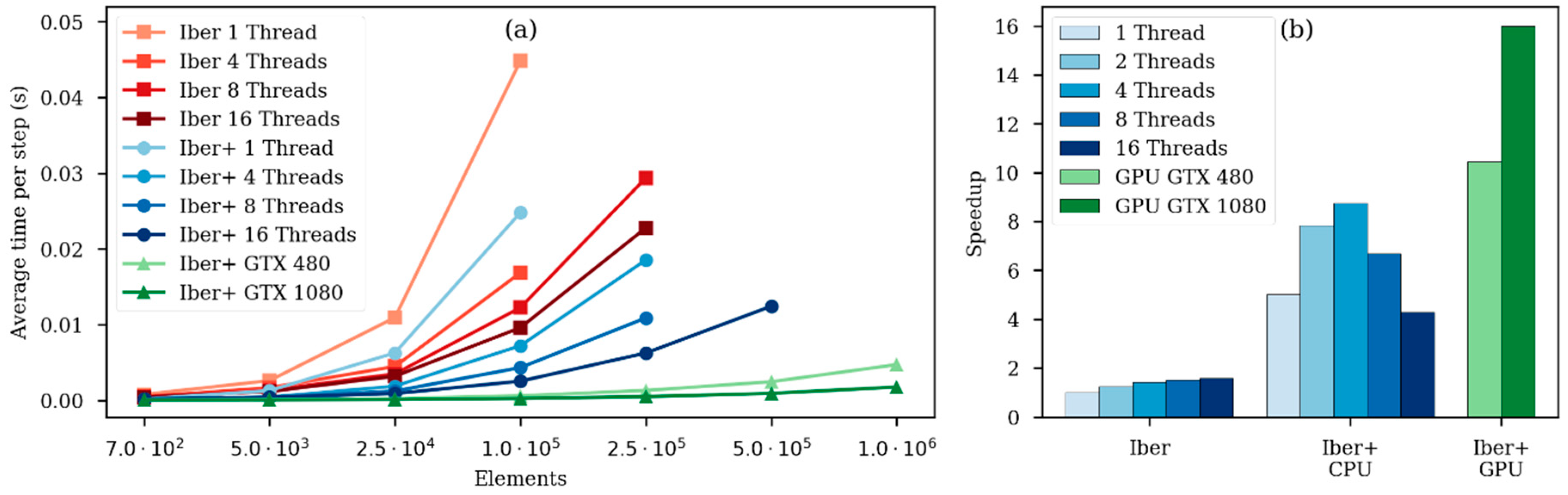
Table 2 shows that the fastest code is Iber+ running on the Nvidia GTX 1080 GPU. It runs 16 times faster than Iber. When running on a GTX 480, a similar GPU to those used by InfoWorks and JFlow+, Iber+ is also faster than those codes. Respecting the execution on the CPU, Iber+ runs five times faster than Iber running both on a single thread (see Figure 5b), and 8.8 times faster using four threads. Note that in this test with 16 threads, Iber+ becomes slower compared to using just four threads. Creating a thread is a time-consuming process. Assigning a big workload to each thread will mitigate the overhead of creating the threads because the time needed to process the workload is much larger than the time used to create the threads. On the other hand, the less workload each thread has, the more significant the overhead in the overall run time. In this case, the mesh has only 700 elements, so if there are many threads involved, each thread has a very small workload. As shown in Figure 5b, there is almost no benefit in using four versus two threads. Moreover, using eight threads is slower than using two, and using 16 threads is even slower than a single thread.
This specific case will be studied in detail to show that the benefits of using parallel executions increases as the mesh size gets bigger. This case was simulated using mesh with different characteristic lengths. As we reduce the element size in the mesh, the Courant [27] increases so the number of steps needed to complete the simulation increases as well. Therefore, the total run-time is not an appropriate metric to analyze the effect of the mesh size on the advantages of parallelization. An alternative metric to analyze this effect is the average execution time per step, defined as the total run-time over the total number of time steps. As shown in Figure 5a, the use of more threads in CPU computations or GPU computing improves the runtime when the number of nodes (elements) increases, since the overhead due to parallelism becomes less significant.
The overhead produced by using parallelism can be measured with the method proposed in [28]. Therefore, the overhead of a parallel region of the code could be defined as Tn − Ts/n, where Tn is the execution time using n processors and Ts is the execution time of the sequential version of the code. For the case with a mesh of 700 elements, the overhead using four threads represents 52% of the total run time, while using 16 threads, it represents 92% of the total run time. On the other hand, in the case with a mesh of 100,000 elements, the overhead using four and 16 threads supposes 13% and, respectively, 37% of the total run time.
3.2. Test 2: Filling of Floodplain Depressions
3.2.1. Case Description
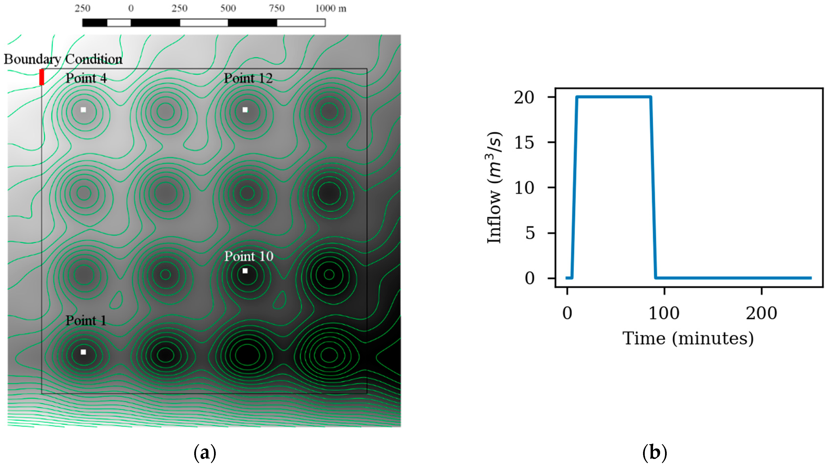
The second test evaluates how the models reproduce the flooding of several depressions that are interconnected. The final distribution of the water is essential to predict the extension of a flood. The topography is a 2000 m × 2000 m domain with a grid of 4 × 4 ground depressions and a slight descending slope in the down-right direction as shown in Figure 6a. The domain is discretized using a structured grid with an element size of 20 m, which gives a numerical grid of 10,000 elements. The Manning’s coefficient is constant and equal to 0.03 s/m1/3 in the entire domain. The initial condition is a completely dry bed. The inlet boundary (red line in Figure 6a) is defined at the top left corner of the domain. The inlet hydrograph is shown in Figure 6b. The total physical time is 48 h. The model outputs to be evaluated are the time series of the water level at the four control points shown in Figure 6a.
3.2.2. Results
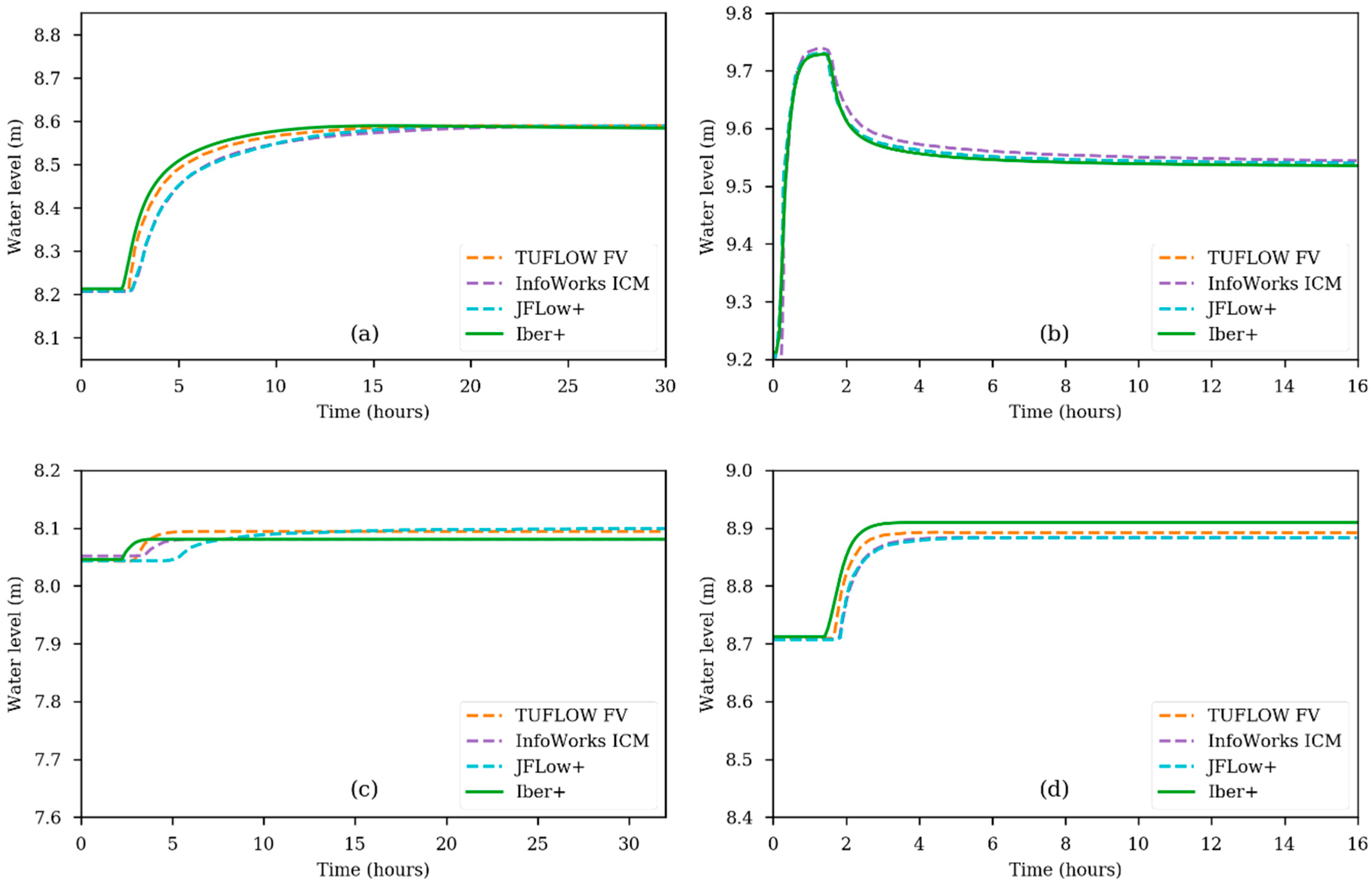
In the original benchmark, the water level evolution was measured at 16 points; for this work and for the sake of clarity, more representative control points were selected. There are no noticeable differences between Iber and Iber+ (in both the CPU and the GPU implementations). Regarding the comparison with other software packages, some differences appear at Point 1 in the arrival time of the flood wave (Figure 7a). JFlow+ and InfoWorks ICM perform similarly, while TUFLOW FV and Iber+ predict a slightly faster propagation of the flood wave. In any case, the final water levels are almost the same for all models. At Point 4, all the models predict very similar results, with the exception of InfoWorks ICM, which shows slightly higher water levels (Figure 7b). At Point 10 (Figure 7c), the highest differences between the analyzed numerical models are shown. The final water level is similar but a bit lower in Iber+. The arrival times also differ, with Iber+ being faster but similar to TUFLOW FV and InfoWorks ICM. Finally, at Point 12 (Figure 7d), small differences in arrival time are shown, as previously reported for Point 1. In general, the models in which the flood arrives earlier also show higher final water levels.
Summarizing, in this case all the models produce very similar results. All of them predict the inundation of 11 out of 16 depressions. Nonetheless, there are some differences on the time of arrival of the water at some depressions. These differences were also noticed in [21] and were attributed to the weak flow between depressions. In these situations, the specific numerical schemes used to discretize the bed slope, the bed friction and the convective flux can have a significant impact on the model output.
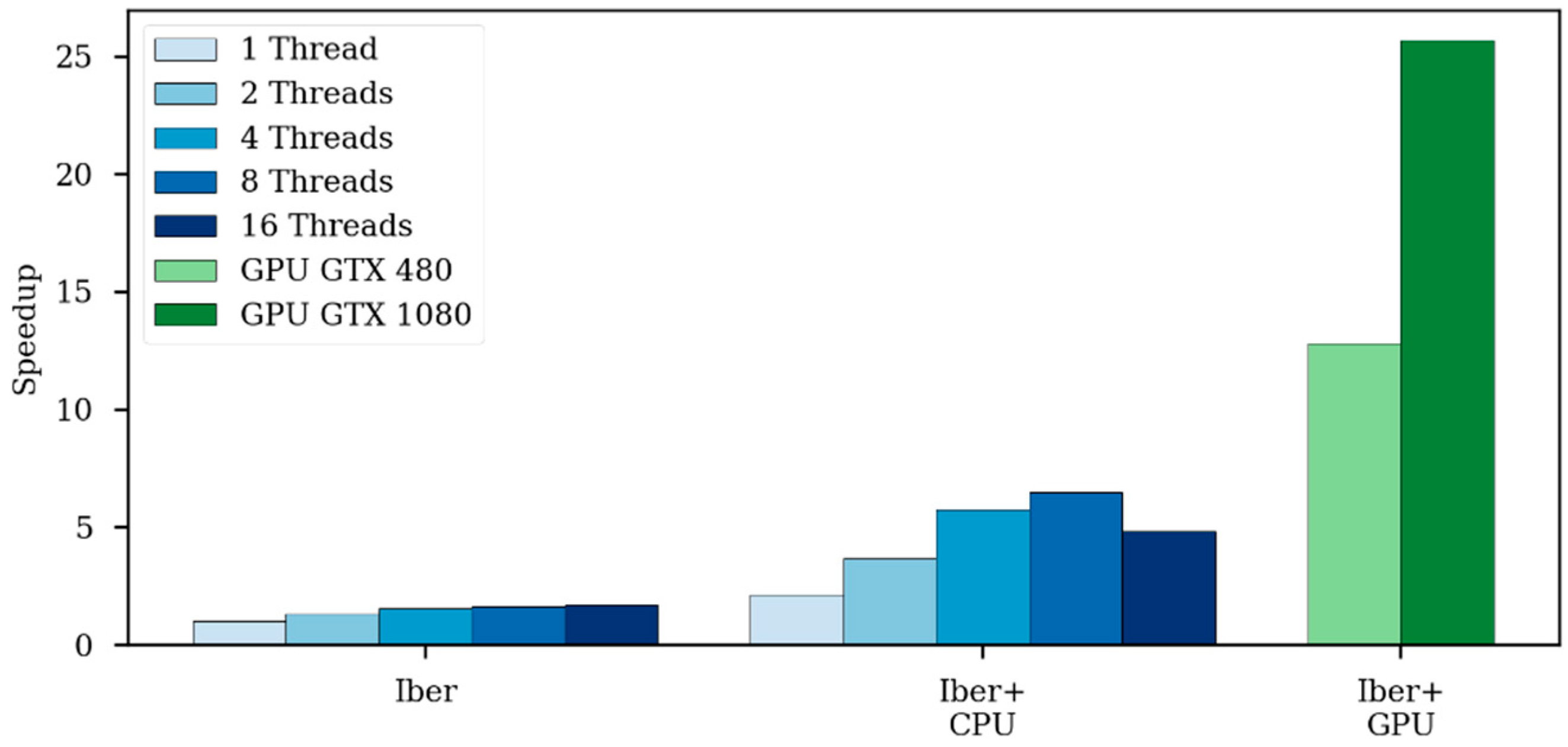
Table 3 shows the computational efficiency of the different models in this test case. Iber+ obtains a speedup of up to 25.7 over the single-threaded Iber. In this case, InfoWorks ICM and JFlow+ are slightly faster than Iber+. Although this case is more complex than Test 1, Iber+ is not able to get any improvement when scaling from eight to 16 threads (Figure 8). This means that for this case, the parallelism overhead is still significant when using 16 threads.
3.3. Test 5: Valley Flooding
3.3.1. Case Description
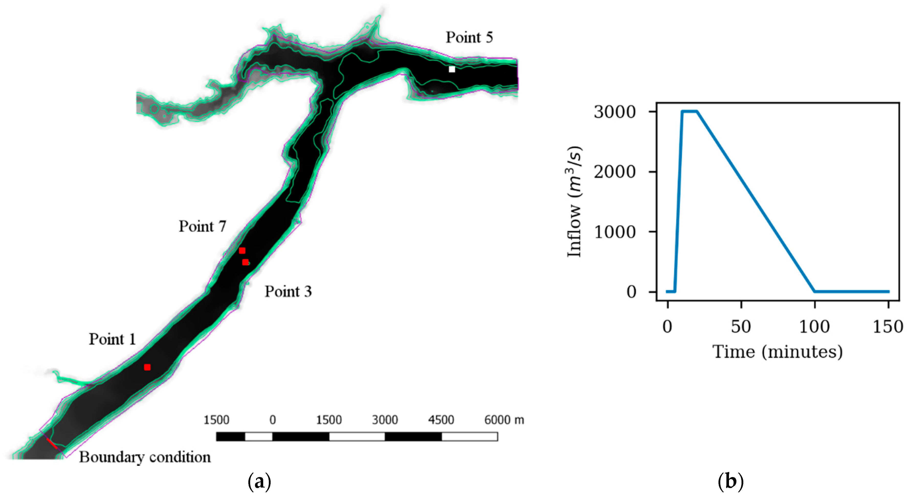
Test 5 consists of a dam break flow that originates a violent flood propagating through a river valley. This case is designed to check the capacity of the models to simulate large inundations. The spatial extension of this case is approximately 0.8 km × 17 km, as shown in Figure 9a. The spatial domain is discretized with an unstructured grid with a characteristic length of approximately 50 m, and a total number of mesh elements of 7753. The Manning’s coefficient is set to 0.04 s/m1/3. The initial condition is a fully dry bed. The inlet boundary condition is marked with a red line in Figure 9a, while the inlet hydrograph is shown in Figure 9b. The physical time in this case is 30 h. The time series of the water levels and velocities at the four control points shown in Figure 9a are used to evaluate and compare the different models.
3.3.2. Results
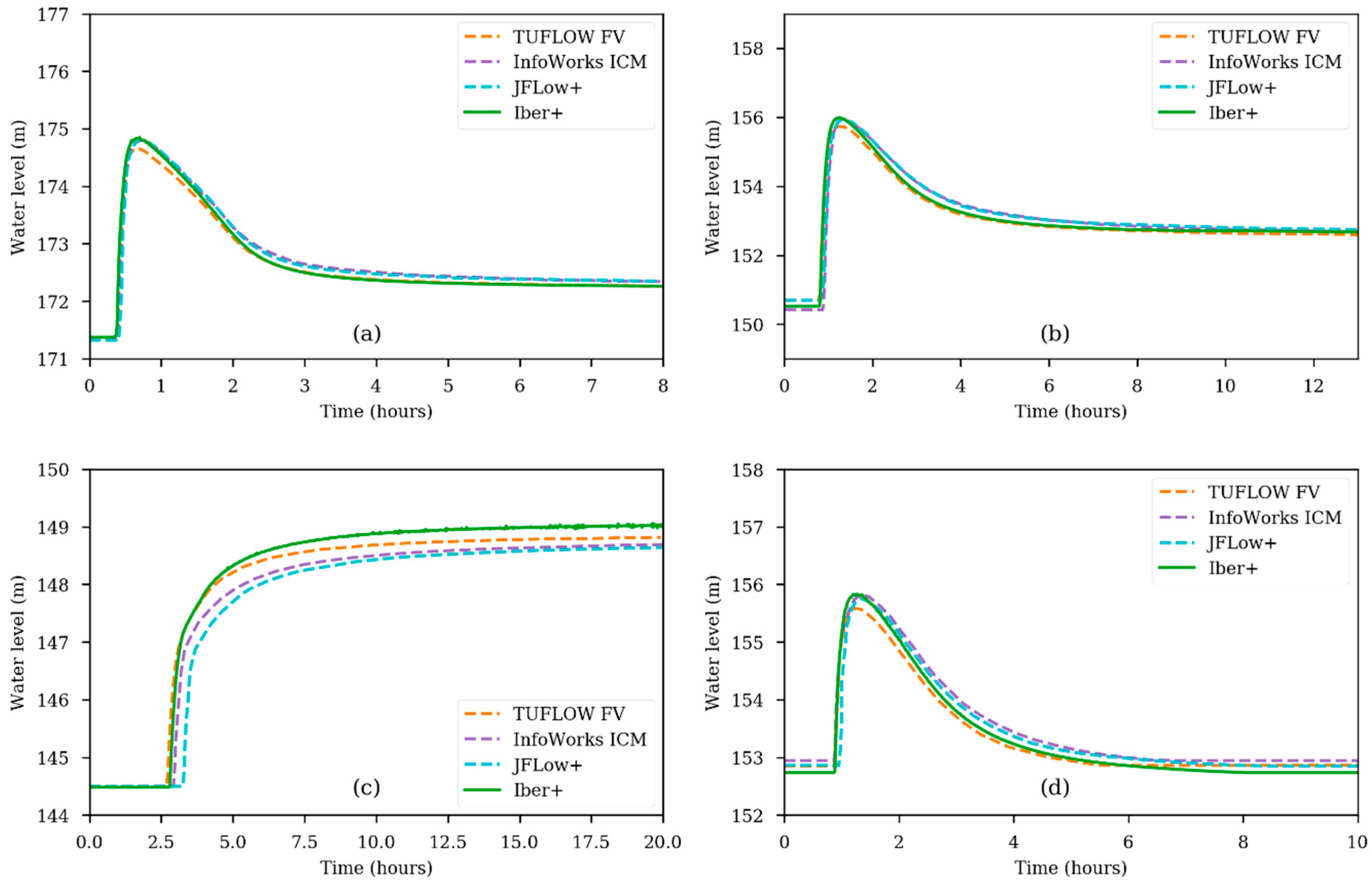
The water levels given by all the models at Points 1, 3 and 7 are very similar (Figure 10). However, some differences can be found at the end of the valley (Point 5), with a delay in the order of 30 min on the time of arrival computed with the different models. Regarding the final water level at Point 5, Iber and Iber+ show values higher than the rest of the models, while InfoWorks ICM and JFlow+ show lower values than TUFLOW FV.
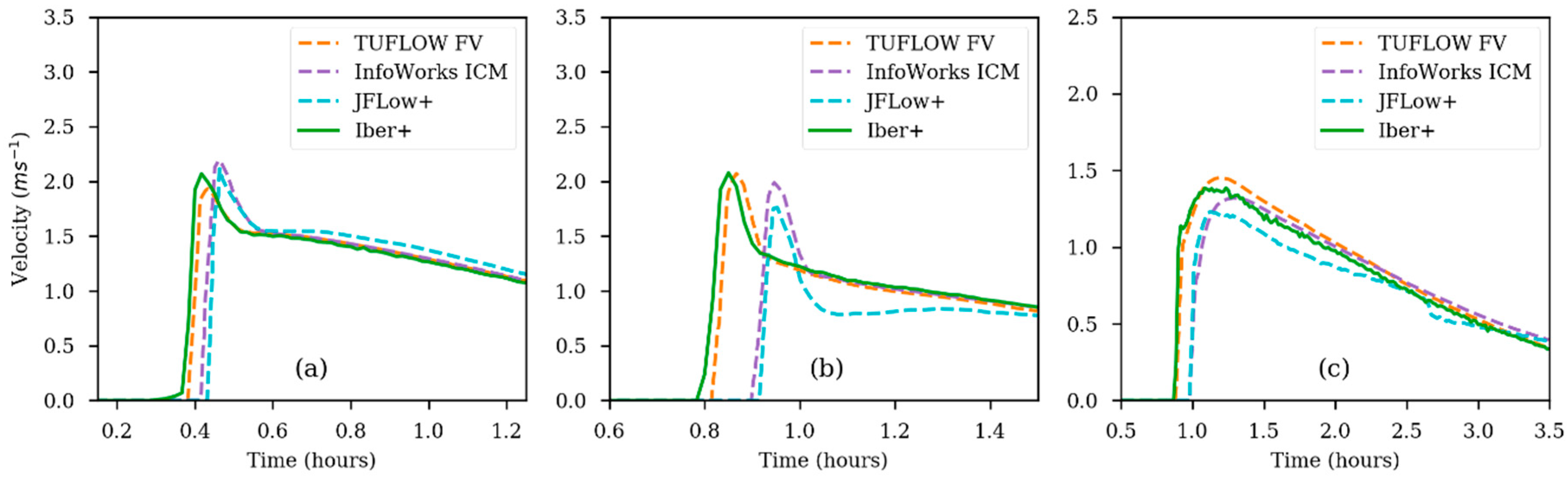
Figure 11 shows the velocity time series at three control points. Iber+ behaves very similar to TUFLOW FV, while InfoWorks ICM and JFlow+ show delays in the arrival times with respect to TUFLOW FV and Iber+ at Point 1 and Point 3.
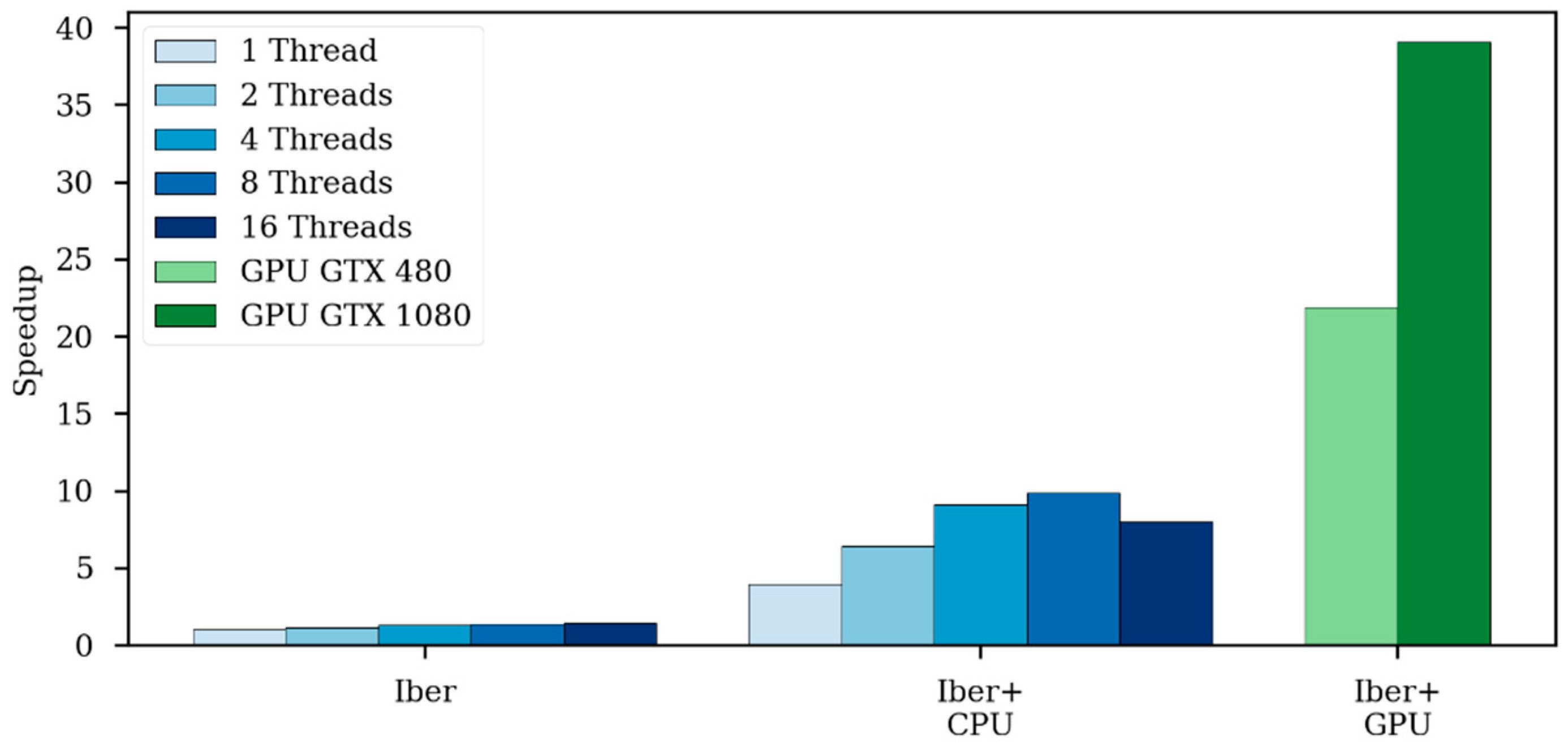
Table 4 shows the computational efficiency of the analyzed models in this case. Iber+ reaches a speedup of 39.1 compared with Iber running in a single thread. In this case, Iber+ runs faster than InfoWorks ICM and JFlow+ using the GTX 1080, but is slower than InfoWorks ICM using the older GTX 480 card. Figure 12 shows a similar behavior as previously observed in Figure 8. Using 16 threads results in worse run times than using just eight threads. This is due to the low number of elements in Test 2 and Test 5.
3.4. Test 8A: Urban Flood
3.4.1. Case Description
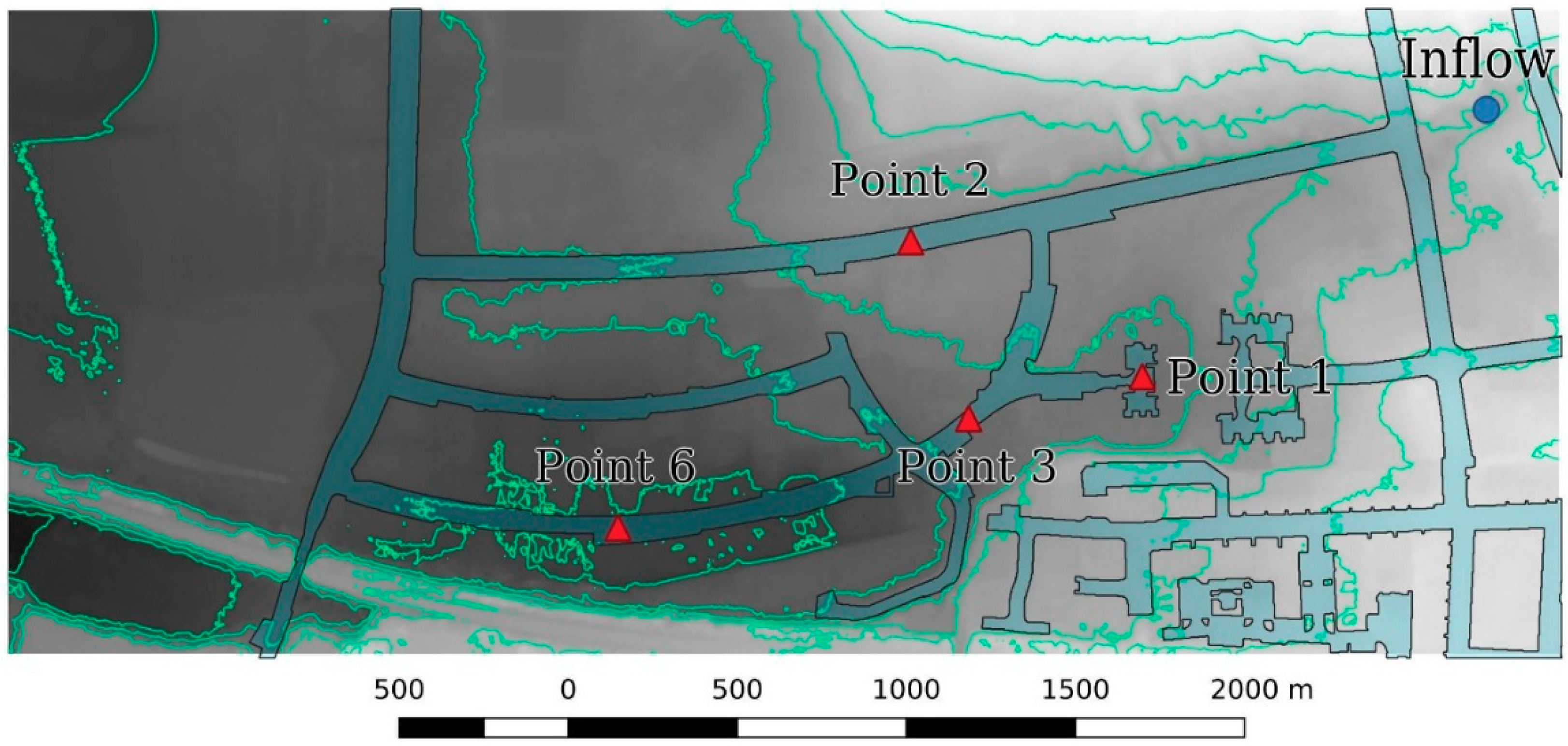
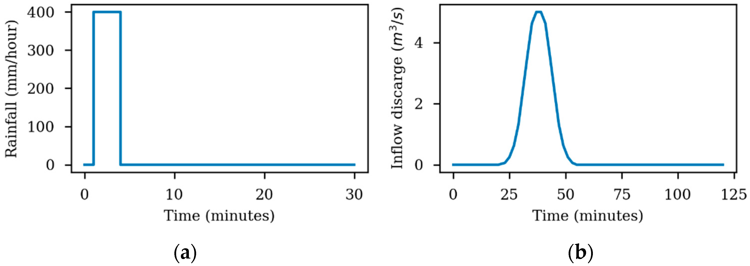
Test 8A simulates an inundation in an urban area of approximately 400 m × 960 m (Figure 13). The topography is defined from a DTM (digital terrain model) with a spatial resolution of 0.5 m. Buildings and vegetation are not included in the DTM and are ignored in the simulation. In this case, the flooding originates from two water sources. A short and intense rainfall event, with intensities up to 400 mm/h, is first defined for the entire domain, and followed by a point inflow hydrograph (blue dot in Figure 13). The hyetograph and the inlet hydrograph are shown in Figure 14a,b. The physical time of the simulation is 3 h. In order to compare the numerical models, the time series of the water levels are extracted at the four control points shown in Figure 13. The time series of velocity at Points 2 and 6 are also analyzed. In this case, the spatial domain is discretized with a structured mesh with a grid resolution of 2 m, which gives a mesh of 96,400 quadrilateral elements.
3.4.2. Results
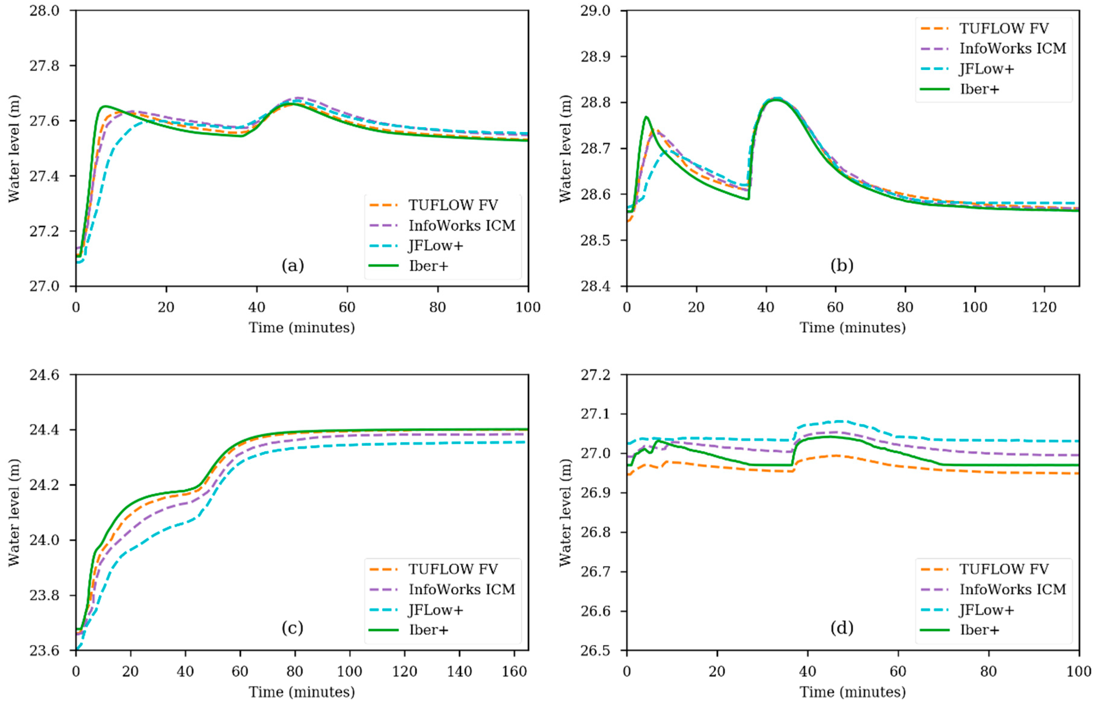
The time series of the water level at Points 1, 2, 3 and 6 are shown in Figure 15. No significant differences were found between Iber and Iber+ CPU/GPU. At Point 1 (Figure 15a) and Point 2 (Figure 15b), the results obtained with Iber+ are very similar to those given by the rest of the models. However, the first peak, caused by the precipitation event, is more pronounced in Iber+ than in the rest of the numerical models. At Point 3 (Figure 15c), Iber+ provides similar results to TUFLOW FV. InfoWorks ICM and JFlow+ produce water levels slightly lower than those obtained using Iber+. At the last point (Point 6 in Figure 15d), Iber+ shows water levels between those provided by TUFLOW FV and InfoWorks ICM.
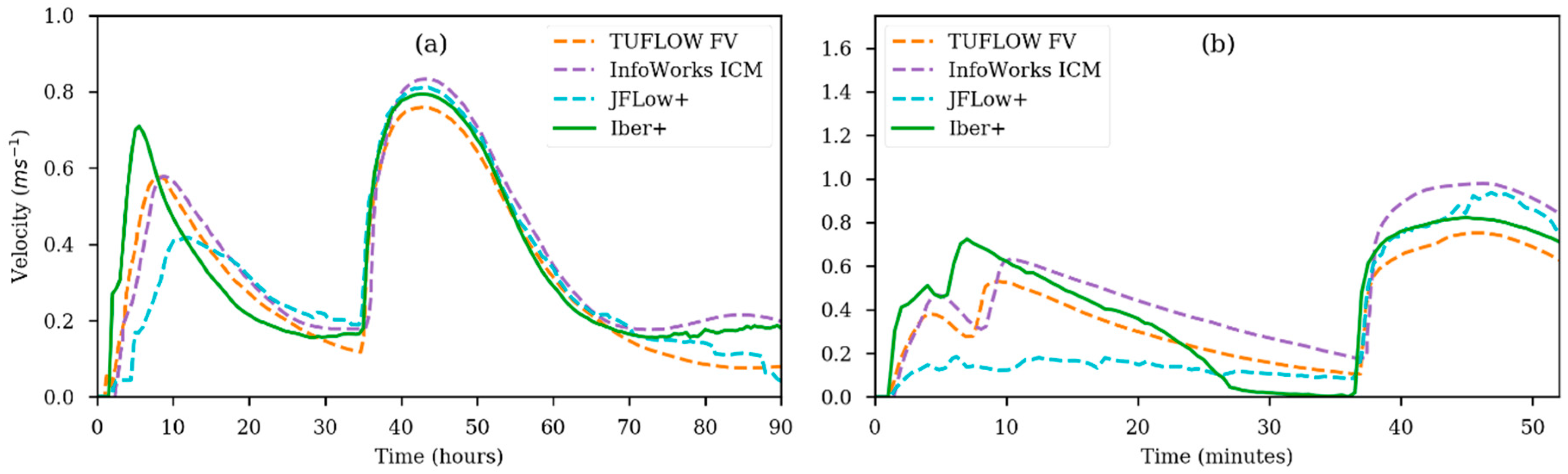
The velocity time series at Points 2 and 6 are shown in Figure 16. Velocities measured at Point 2 are similar for all the models, and the differences are in concordance with the differences seen in the water levels and arrival times for that point. However, at Point 2, with lower water depths, there are more differences among models.
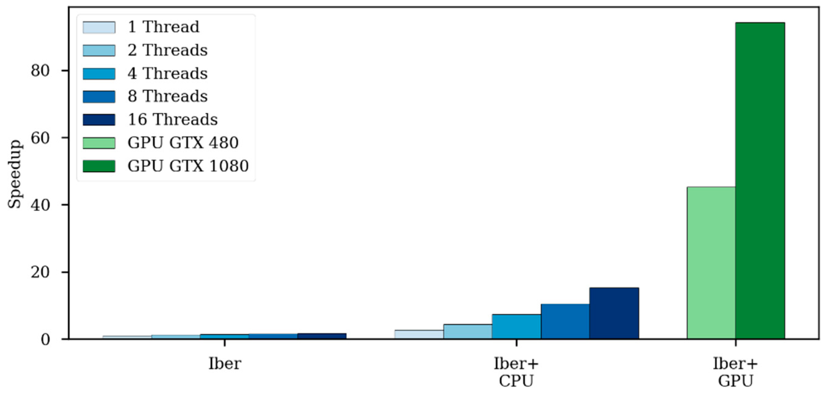
Table 5 shows the computational efficiency of the different models in this test case. Since this case is more complex and has many more elements than the previous ones, it has a higher benefit from GPU implementation, running up to 94 times faster than Iber on a single CPU (Figure 17). Compared with other models from [21], in this case, the Iber+ GPU is slightly faster than InfoWorks and JFlow+ using a GPU with similar specifications (GTX 480).
4. Application Case: Surface Runoff Generation in a Mountain Basin during a Storm Event
In this section, a real fast flood event due to heavy precipitation in a mountain basin was used to verify the computational performance of Iber+ in large scale simulations. The discharge computed with Iber+ is compared with observed data registered during the real event at a gauging station located at the basin outlet. The run times of Iber and Iber+ are also compared. The simulations were run with a CPU Intel Core i7-920 and with a GPU NVIDIA GeForce GTX 1080.
4.1. Case Description
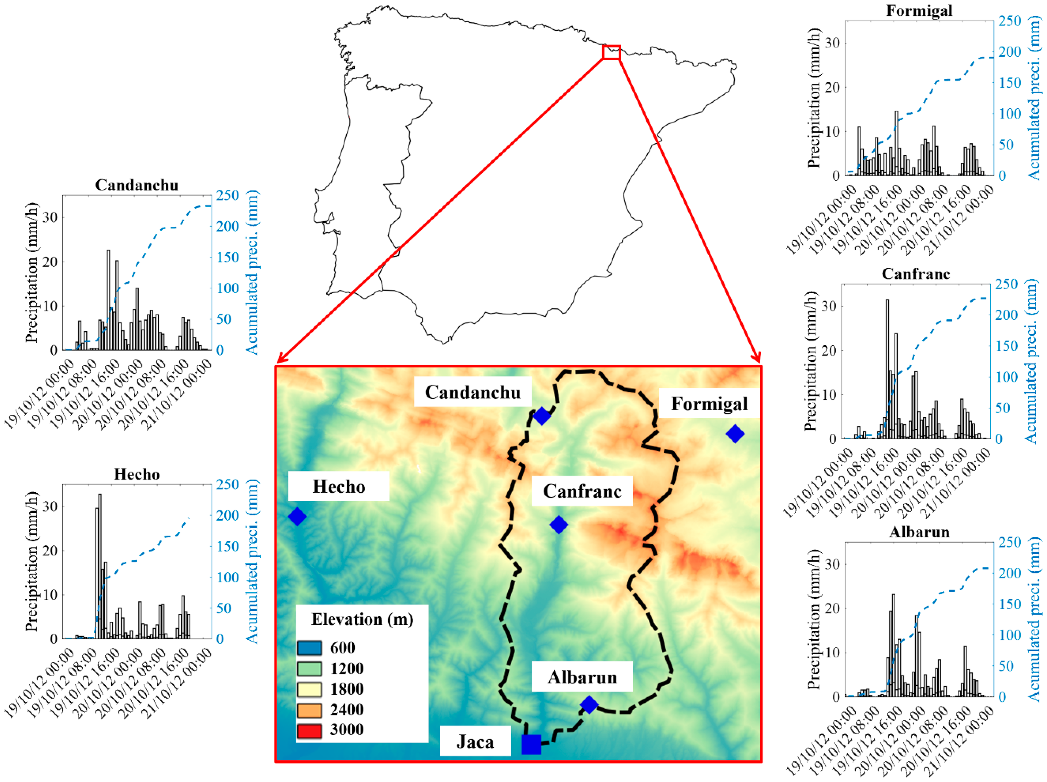
On 19–21 October 2012, an extreme rainfall event was observed in the central western Pyrenees, affecting mainly the headwater catchments of the Aragón river [29,30]. This basin is located in north-eastern Spain, near the Mediterranean Sea and in the Pyrenees mountain range, and is prone to flooding during autumn. Precipitation events of more than 200 mm in just a few hours have been reported by various authors in that area [18,19]. Figure 18 shows the location of the Upper Aragón basin, which has an area of around 240 km2 and altitudes ranging from approximately 600 m to 3000 m. Figure 18 also shows the location of five rain gauges (Candanchu, Hecho, Formigal, Canfranc and Albarun) operated by the Ebro River Basin Authority (CHEbro), and the hyetographs recorded by these gauges on 19–21 October 2012. Three of these rain gauges (Candanchu, Canfranc and Albarun) are located inside the study catchment. The observed hyetographs show peak values close to 25 mm/h on 19 October. The rain gauges at Hecho and Canfranc registered peak values of more than 30 mm/h during the first hours of 19 October. The rain gauge at Formigal, which is the eastern-most gauge, recorded peak values smaller than 20 mm/h. The accumulated precipitation of the rain gauges ranged from 200 mm at Formigal to near 250 mm at Candanchu. These values are more than three times higher than the monthly averaged accumulated precipitation of October over the period of 1981–2010 (60 mm) registered at the AEMET (Agencia Estatal de Meteorología) rain gauge located at Huesca airport (available online at http://www.aemet.es/es/serviciosclimaticos/datosclimatologicos/). The discharge of the Aragón river registered at the town of Jaca was used for comparison with the numerical results.
A series of simulations were carried out with Iber+ in order to compute the discharge at the gauge station of Jaca during the first 24 h of this extreme event. The numerical domain was discretized using triangular elements with a characteristic length ranging from 5 m near the riverbed, to 40 m. This led to a mesh of 459,000 elements. The wet-dry threshold was set equal to 0.001 m. The hydrodynamic equations were discretized using the DHD scheme [6], which is especially designed for solving the shallow water equations in rainfall–runoff applications. The physical time of the simulation was 24 h. The hyetographs registered at the five rain gauges (Figure 18) were spatially interpolated to define precipitation rasters that were used as the rainfall input in the numerical model.
The Manning coefficient was also provided to Iber+ as a raster file. The raster file of the Manning coefficients was obtained starting from shape files of land uses of the SIOSE (Sistema de Información sobre Ocupación del Suelo de España) downloaded from the web of the CNIG (Centro Nacional de Información Geográfica). These shape files divide the entire area of study into small parcels (j = 1, …, N), each of them with a combined land use, which was labelled according the rules of SIOSE by the type of parcel, individual land uses defined in each parcel and the ratio of area of each individual land use to the total area of the parcel. Each individual land use is associated to a Manning coefficient obtained from [6]. The combined Manning coefficient of each parcel j was obtained using:
where Perij is the ratio of land use i in parcel j (∈ [0,1]), Ci is the Manning coefficient associated to the land use i, Mj is the number of land uses in the parcel j. Details of the methodology to compute the Manning coefficients can be found in [31].
Infiltration losses were defined using the curve number method of the SCS (Soil Conservation Service). The curve number (CN) was computed with the formulation proposed in [32]. First, the maximum surface retention (S) was obtained as:
where Ru is the mean value of surface runoff and P the precipitation depth both provided as raster files. From the maximum surface retention, the curve number was estimated as:
There are multiple sources of uncertainty in numerical models. Apart from the limitations in the model formulation, especially those related to the mathematical discretization of the equations, the models are very sensitive to the initial boundary conditions, as well as to the input parameters. In the particular case of hydraulic models like Iber, the parameterization of the Manning coefficients and CN are of utmost importance in order to determine the timing and extent of flooding events. In the present case, the reference simulation described above and a set of 16 additional simulations were considered. Among them, eight simulations were defined by the reference CN and varying Manning coefficients (±15%, ±35%, ±55% and ±75%) and eight simulations were defined by the reference Manning coefficients and varying curve number (±3%, ±6%, ±9% and ±12%).
4.2. Results
Figure 19 shows the averaged hydrograph computed with Iber+ and the experimental values observed at Jaca. The shaded area corresponds to the mean value plus/minus two times the standard deviation of the numerical simulations. The average peak discharge obtained with Iber+ is slightly higher (~25%) than the experimental one (349.5 m3 s−1 and 279.5 m3 s−1 respectively). The difference between both values (70.0 m3 s−1) is considerably lower than twice the standard deviation (shaded area). The timing of the numerical peak (20.0 h) is slightly delayed with respect to the observed data (19.5 h). The total volume of water also shows slight differences (~2%) between the experimental (4.6 Hm3) and numerical (4.7 Hm3) results. Therefore, the model reproduces the observed data with an acceptable accuracy, especially considering the uncertainty inherent to hydrological simulations.
In addition to the visual comparison derived from Figure 19, three non-dimensional quantitative statistics and two dimensional techniques have been used to evaluate, in an objective way, the accuracy of the numerical results compared to the field data. The non-dimensional quantitative statistics used are the Nash–Sutcliffe efficiency (NSE), percent bias (PBIAS) and the ratio of the root mean square error to the standard deviation of measured data (RSR). The used dimensional techniques are the correlation coefficient (r) and the coefficient of determination (R2). The Nash–Shutcliffe coefficient (NSE) [33] defines the relation of the residual variance to the field data variance. It can range from −∞ to 1 and its optimal value is 1. NSE was used according to the recommendation of [34] and its widespread use in the hydrology field [35,36]. Percent bias (PBIAS) [37] measures the tendency of the numerical results to be larger (PBIAS > 0) or smaller (PBIAS < 0) than the reference data and is expressed as a percentage. Therefore, the optimal value of this parameter is 0. This parameter is also recommended by [34] and, according to [37], it can identify numerical models with poor accuracy. The ratio of the root mean square error to the standard deviation of measured data (RSR) [38] is defined as the ratio of root mean square error (RMSE) to the standard deviation of the field data. It can range from 1 to a large positive number. In the former case, the RMSE would be equal to the standard deviation of the field data and in the latter case, the RMSE would be greater than the standard deviation of the field data.
Following [39], the range of values of the non-dimensional statistics is shown in Table 6. Note that these values are defined for monthly time steps. Usually as the time step decreases, the ratings are less stringent.
Table 7 shows the values of the statistics parameters obtained for the case under study. The values of NSE, PBIAS and RSR clearly indicate, according to the reference values of Table 6, that the accuracy of the numerical results is very good. In addition, the values of r and R2 show the high accuracy of the numerical model.
Apart from the accuracy of the results, this case study highlights the need for computationally efficient models. The total runtime needed for the 17 numerical simulations was approximately two hours and twenty minutes (approximately eight minutes per simulation). The time needed to run the same case with the standard Iber ranged from 14 h 25 min with eight threads and 18 h 9 min with one thread. We should note that weather forecast systems can predict extreme rain events only a few hours in advance, which reduces the response time and highlights the need for fast and reliable hydraulic models to analyze the areas at risk of flooding. Iber+ can then be considered as a suitable tool to predict these type of extreme events.
5. Conclusions
We have presented a new parallel implementation of the 2D shallow water model Iber. The new implementation, named Iber+, takes advantage of different parallelization strategies both on CPUs and GPUs to speed up the computations, while keeping the same accuracy as the original model. The computational efficiency of the new code was analysed using four different benchmarks proposed by the Environmental Agency of the United Kingdom. The results obtained with Iber+ on those benchmarks was compared to those given by other hydraulic models, showing a similar level of accuracy.
The main limitation of the standard implementation of Iber is its lack of computational efficiency in large problems. This limitation is overcome in the new parallel implementation, where a speedup of two orders of magnitude, compared to the standard version, can be obtained depending on the case under study. This speedup is especially relevant on the GPU version of the code when modelling cases with a high workload.
Iber+ was applied to a real case, an extreme flash flood that took place in the Spanish Pyrenees in October 2012. Iber+ was able to simulate 24 h of physical time in less than 10 min using a numerical mesh of almost half a million elements. The same case run with the standard version needs more than 15 h of CPU time. This improvement in computational time is especially important to extend the potential application of the model to early warning systems, since extreme precipitation events can only be forecasted a few hours in advance by the meteorological agencies. Thus, the use of fast and accurate numerical tools such as Iber+ is crucial for a real-time analysis and deployment of flood protection measures by decision makers.
Although Iber+ offers a huge performance leap compared to the standard version, there is still room for further speedups by the use of ordering algorithms for data locality, the improvement in the efficiency to skip dry elements from the computation, or the implementation of asynchronous tasks in GPU programming.
Author Contributions
O.G.-F., J.G.-C., M.G.-G. and J.M.D. conceived the study; O.G.-F. developed the software; L.C., J.M.D. and A.F. supervised the code development; O.G.-F. and J.G.-C. performed the experiments; O.G.-F., J.G.-C. and M.G.-G. analysed the results; O.G.-F., J.G.-C., L.C., M.G.-G. and A.F. wrote the manuscript.
Funding
This research was partially supported by Water JPI—WaterWorks Programme under project Improving Drought and Flood Early Warning, Forecasting and Mitigation (IMDROFLOOD) (Code: PCIN-2015-243); by INTERREG-POCTEP Programme under project RISC_ML (Code: 0034_RISC_ML_6_E); and by Xunta de Galicia under Project ED431C 2017/64-GRC “Programa de Consolidación e Estruturación de Unidades de Investigación Competitivas (Grupos de Referencia Competitiva)”. O.G.-F. is supported by Xunta de Galicia grant ED481A-2017/314. J.M.D. is supported by Xunta de Galicia postdoctoral grant ED481B-2018/020.
Acknowledgments
We acknowledge CHMS for the availability of the raster files of mean value of surface runoff and precipitation depth.
Conflicts of Interest
The authors declare no conflict of interest. The founding sponsors had no role in the design of the study, in the collection, analyses and interpretation of data, in writing of the manuscript and in the decision to publish the results.
Abbreviations
| AEMET | Agencia Estatal de Meteorología. |
| API | Application Programming Interface |
| AVX | Advanced Vector Extensions |
| CHEbro | Confederación Hidrográfica del Ebro. |
| CHMS | Confederación Hidrográfica Miño Sil. |
| CNIG | Centro Nacional de Información Geográfica |
| CPU | Central Processing Unit |
| CUDA | Compute Unified Device Architecture |
| CUB | CUDA Unbound |
| DHD | Decoupled Hydrological Discretization |
| DTM | Digital Terrain Model |
| GPGPU | General Processing Graphics Processing Unit |
| GPU | Graphics Processing Unit |
| I/O | Input/Output |
| MPI | Message Passing Interface |
| OpenMP | Open Multi-Processing |
| PCI | Peripheral Component Interconnect |
| RMSD | Root Mean Square Deviation |
| SCS | Soil Conservation Service |
| SIMD | Single Instruction Multiple Data |
| SIMT | Single Instruction Multiple Thread |
| SIOSE | Sistema de Información sobre Ocupación del Suelo de España. |
| SM | Streaming Multiprocessors |
| SWE | Shallow Water Equations |
| SSE | Streaming SIMD Extensions |
References
- Houghton, J.T.; Ding, Y.; Griggs, D.J.; Noguer, M.; van der Linden, P.J.; Dai, X.; Maskell, K.; Johnson, C.A. Climate Change 2001: The Scientific Basis; Cambridge University Press: Cambridge, UK, 2001; ISBN 9780521014953. [Google Scholar]
- Hov, Ø.; Cubasch, U.; Fischer, E.; Höppe, P.; Iversen, T. Extreme Weather Events in Europe: Preparing for Climate Change Adaptation; Norwegian Meteorological Institute: Oslo, Norway, 2013. [Google Scholar]
- Bladé, E.; Cea, L.; Corestein, G.; Escolano, E.; Puertas, J.; Vázquez-Cendón, E.; Dolz, J.; Coll, A. Iber: Herramienta de simulación numérica del flujo en ríos. Rev. Int. Métodos Numéricos para Cálculo y Diseño en Ing. 2014, 30, 1–10. [Google Scholar] [CrossRef]
- Cea, L.; Bermudez, M.; Puertas, J.; Blade, E.; Corestein, G.; Escolano, E.; Conde, A.; Bockelmann-Evans, B.; Ahmadian, R. IberWQ: New simulation tool for 2D water quality modelling in rivers and shallow estuaries. J. Hydroinform. 2016. [Google Scholar] [CrossRef]
- Roe, P.L. Discrete Models for the Numerical Analysis of Time-Dependent Multidimensional Gas Dynamics. In Upwind and High-Resolution Schemes; Springer: Berlin/Heidelberg, Germany, 1986; pp. 451–469. [Google Scholar] [Green Version]
- Cea, L.; Bladé, E. A simple and efficient unstructured finite volume scheme for solving the shallow water equations in overland flow applications. Water Resour. Res. 2015, 51, 5464–5486. [Google Scholar] [CrossRef] [Green Version]
- Bladé Castellet, E.; Cea, L.; Corestein, G. Numerical modelling of river inundations. Ingeniería del Agua 2014, 18, 68. [Google Scholar] [CrossRef] [Green Version]
- Bodoque, J.M.; Amérigo, M.; Díez-Herrero, A.; García, J.A.; Cortés, B.; Ballesteros-Cánovas, J.A.; Olcina, J. Improvement of resilience of urban areas by integrating social perception in flash-flood risk management. J. Hydrol. 2016, 541, 665–676. [Google Scholar] [CrossRef] [Green Version]
- Cea, L.; French, J.R. Bathymetric error estimation for the calibration and validation of estuarine hydrodynamic models. Estuar. Coast. Shelf Sci. 2012, 100, 124–132. [Google Scholar] [CrossRef]
- Fraga, I.; Cea, L.; Puertas, J.; Suárez, J.; Jiménez, V.; Jácome, A. Global Sensitivity and GLUE-Based Uncertainty Analysis of a 2D-1D Dual Urban Drainage Model. J. Hydrol. Eng. 2016, 21, 04016004. [Google Scholar] [CrossRef]
- Cea, L.; Legout, C.; Grangeon, T.; Nord, G. Impact of model simplifications on soil erosion predictions: Application of the GLUE methodology to a distributed event-based model at the hillslope scale. Hydrol. Process. 2016. [Google Scholar] [CrossRef]
- Sopelana, J.; Cea, L.; Ruano, S. A continuous simulation approach for the estimation of extreme flood inundation in coastal river reaches affected by meso- and macrotides. Nat. Hazards 2018, 93, 1337–1358. [Google Scholar] [CrossRef]
- Crespo, A.J.C.; Domínguez, J.M.; Rogers, B.D.; Gómez-Gesteira, M.; Longshaw, S.; Canelas, R.; Vacondio, R.; Barreiro, A.; García-Feal, O. DualSPHysics: Open-source parallel CFD solver based on Smoothed Particle Hydrodynamics (SPH). Comput. Phys. Commun. 2015, 187, 204–216. [Google Scholar] [CrossRef]
- Crossley, A.; Lamb, R.; Waller, S. Fast Solution of the Shallow Water Equations Using GPU Technology. 2010. Available online: http://www.jflow.co.uk/sites/default/files/Crossley%20Lamb%20Waller%20-%20BHS%202010.pdf (accessed on 9 October 2018).
- Vacondio, R.; Dal Palù, A.; Mignosa, P. GPU-enhanced finite volume shallow water solver for fast flood simulations. Environ. Model. Softw. 2014. [Google Scholar] [CrossRef]
- Lacasta, A.; Morales-Hernández, M.; Murillo, J.; García-Navarro, P. An optimized GPU implementation of a 2D free surface simulation model on unstructured meshes. Adv. Eng. Softw. 2014. [Google Scholar] [CrossRef]
- Liu, Q.; Qin, Y.; Li, G. Fast Simulation of Large-Scale Floods Based on GPU Parallel Computing. Water 2018, 10, 589. [Google Scholar] [CrossRef]
- NVIDIA Corporation. CUDA C Programming Guide. Available online: https://docs.nvidia.com/cuda/pdf/CUDA_C_Programming_Guide.pdf (accessed on 25 September 2018).
- Merry, B. A Performance Comparison of Sort and Scan Libraries for GPUs. Parallel Process. Lett. 2015, 25, 1550007. [Google Scholar] [CrossRef] [Green Version]
- NVIDIA Corporation. GP100 Pascal Whitepaper. Available online: https://images.nvidia.com/content/pdf/tesla/whitepaper/pascal-architecture-whitepaper.pdf (accessed on 9 October 2018).
- Neelz, S.; Pender, G. Delivering Benefits through Evidence-Benchmarking of 2D Hydraulic Modelling Packages; Environment Agency: Bristol, UK, 2010; ISBN 9781849111904.
- TUFLOW FV Science Manual. Available online: https://www.tuflow.com/Download/TUFLOW_FV/Manual/FV_Science_Manual_2013.pdf (accessed on 10 September 2018).
- InfoWorks ICM Product Information—Overview. Available online: http://www.innovyze.com/products/infoworks_icm/ (accessed on 10 September 2018).
- Néelz, S.; Pender, G.; Britain, G. Desktop Review of 2D Hydraulic Modelling Packages; Environment Agency: Bristol, UK, 2009; ISBN 9781849110792.
- Anzt, H.; Hahn, T.; Heuveline, V. GPU Accelerated Scientific Computing: Evaluation of the NVIDIA Fermi Architecture; Elementary Kernels and Linear Solvers; EMCL: Heidelberg, Germany, 2010. [Google Scholar]
- Gregg, C.; Hazelwood, K. Where is the data? Why you cannot debate CPU vs. GPU performance without the answer. In Proceedings of the ISPASS 2011—IEEE International Symposium on Performance Analysis of Systems and Software, Austin, TX, USA, 10–12 April 2011. [Google Scholar]
- Courant, R.; Friedrichs, K.; Lewy, H. Über die partiellen Differenzengleichungen der mathematischen Physik. Math. Ann. 1928. [Google Scholar] [CrossRef]
- Bull, J.M. Measuring Synchronisation and Scheduling Overheads in OpenMP. In Proceedings of the First European Workshop on OpenMP, 1999; Available online: http://cc.jlu.edu.cn/Download/4c09bb4a-8dae-4083-acd3-052c4eb8ad61.pdf (accessed on 15 October 2018).
- Naverac, V.; Ferrer, D.; Curiel, P.; Zueco, S.D.; Gil, F.E.; Hidalgo, J.C.G.; García, D.G.; de Matauco, A.I.G.; Albero, C.M.; Mur, D.M.; et al. Sobre las Precipitaciones de Octubre de 2012 en el Pirineo Aragonés, su Respuesta Hidrológica y la Gestión de Riesgos. 2012. Available online: https://dialnet.unirioja.es/descarga/articulo/4138905.pdf (accessed on 15 October 2018).
- Serrano-Muela, M.P.P.; Nadal-Romero, E.; Lana-Renault, N.; González-Hidalgo, J.C.C.; López-Moreno, J.I.I.; Beguería, S.; Sanjuan, Y.; García-Ruiz, J.M.M. An exceptional rainfall event in the central western pyrenees: Spatial patterns in discharge and impact. Land Degrad. Dev. 2015. [Google Scholar] [CrossRef] [Green Version]
- González-Cao, J.; García-Feal, O.; Crespo, A.J.C.; Gómez-Gesteira, M.; Cea, L. Predicción de Inundaciones Originadas por Precipitaciones Extremas Mediante el Módulo Hidrológico de Iber. 2017. Available online: http://geama.org/jia2017/wp-content/uploads/ponencias/tema_B/b1.pdf (accessed on 15 October 2018).
- Patil, J.P.P.; Sarangi, A.; Singh, A.K.K.; Ahmad, T. Evaluation of modified CN methods for watershed runoff estimation using a GIS-based interface. Biosyst. Eng. 2008. [Google Scholar] [CrossRef]
- Nash, J.E.; Sutcliffe, J.V. River flow forecasting through conceptual models part I—A discussion of principles. J. Hydrol. 1970, 10, 282–290. [Google Scholar] [CrossRef]
- American Society of Civil Engineers. Criteria for Evaluation of Watershed Models. J. Irrig. Drain. Eng. 1993, 119, 429–442. [Google Scholar] [CrossRef]
- Servat, E.; Dezetter, A. Selection of calibration objective fonctions in the context of rainfall-ronoff modelling in a Sudanese savannah area. Hydrol. Sci. J. 1991, 36, 307–330. [Google Scholar] [CrossRef] [Green Version]
- Legates, D.R.; McCabe, G.J. Evaluating the use of “goodness-of-fit” measures in hydrologic and hydroclimatic model validation. Water Resour. Res. 1999. [Google Scholar] [CrossRef]
- Gupta, H.V.; Sorooshian, S.; Yapo, P.O. Status of Automatic Calibration for Hydrologic Models: Comparison with Multilevel Expert Calibration. J. Hydrol. Eng. 1999. [Google Scholar] [CrossRef]
- Singh, J.; Knapp, H.V.; Arnold, J.G.; Demissie, M. Hydrological modeling of the Iroquois River watershed using HSPF and SWAT. J. Am. Water Resour. Assoc. 2005. [Google Scholar] [CrossRef]
- Moriasi, D.N.; Arnold, J.G.; Van Liew, M.W.; Bingner, R.L.; Harmel, R.D.; Veith, T.L. Model Evaluation Guidelines for Systematic Quantification of Accuracy in Watershed Simulations. Trans. ASABE 2007, 50, 885–900. [Google Scholar] [CrossRef]
Figure 1.
Flow chart of Iber+ GPU implementation.

Figure 2.
Simulated domain for Test 1. White areas represent high terrain elevation. To the left, there is an inlet boundary condition. In red, the measurement points.
Figure 2.
Simulated domain for Test 1. White areas represent high terrain elevation. To the left, there is an inlet boundary condition. In red, the measurement points.

Figure 3.
Elevations along the domain. Z stands for elevation in meters and X for horizontal distance from the origin of the channel (a). Hydrograph defined for the inlet boundary condition (b).
Figure 3.
Elevations along the domain. Z stands for elevation in meters and X for horizontal distance from the origin of the channel (a). Hydrograph defined for the inlet boundary condition (b).

Figure 4.
Time series of the water level for Test 1 obtained using all the numerical models at Point 1 (a) and at Point 2 (b).
Figure 4.
Time series of the water level for Test 1 obtained using all the numerical models at Point 1 (a) and at Point 2 (b).

Figure 5.
Average processing time per time step versus the number of elements of the simulated mesh using different configurations (a); Speedups obtained comparing Iber running in one thread with different configurations in Test 1 using a mesh of 700 elements (b).
Figure 5.
Average processing time per time step versus the number of elements of the simulated mesh using different configurations (a); Speedups obtained comparing Iber running in one thread with different configurations in Test 1 using a mesh of 700 elements (b).

Figure 6.
Setup of Test 2. (a) Shows the simulated domain. White areas represent higher elevations. The inlet boundary condition is marked in red. The measurements were performed in the points shown above; (b) Hydrograph used for the inlet boundary condition.
Figure 6.
Setup of Test 2. (a) Shows the simulated domain. White areas represent higher elevations. The inlet boundary condition is marked in red. The measurements were performed in the points shown above; (b) Hydrograph used for the inlet boundary condition.

Figure 7.
Water level time series for Test 2 obtained with different numerical models at Point 1 (a); Point 4 (b); Point 10 (c); Point 12 (d).
Figure 7.
Water level time series for Test 2 obtained with different numerical models at Point 1 (a); Point 4 (b); Point 10 (c); Point 12 (d).

Figure 8.
Speedups obtained comparing Iber running in one thread with different configurations in Test 2.
Figure 8.
Speedups obtained comparing Iber running in one thread with different configurations in Test 2.

Figure 9.
Setup of Test 5. (a) Shows the simulated domain. White areas represent higher elevations and black areas represent lower elevations. Light green lines are level curves. The inlet boundary condition is marked in red. The measurements were performed at the points shown above; (b) Hydrograph used as the upstream inlet boundary condition.

Figure 10.
Time series of water level for Test 5 obtained with different numerical models at Point 1 (a); Point 3 (b); Point 5 (c); and Point 7 (d).
Figure 10.
Time series of water level for Test 5 obtained with different numerical models at Point 1 (a); Point 3 (b); Point 5 (c); and Point 7 (d).

Figure 11.
Time series of velocity for Test 5 obtained with different numerical models at Point 1 (a); Point 3 (b); and Point 7 (c).
Figure 11.
Time series of velocity for Test 5 obtained with different numerical models at Point 1 (a); Point 3 (b); and Point 7 (c).

Figure 12.
Speedups obtained comparing Iber running in one thread with different configurations in Test 5.
Figure 12.
Speedups obtained comparing Iber running in one thread with different configurations in Test 5.

Figure 13.
Setup of Test 8A. White areas represent higher elevations. Measurement points are marked in red. A point inflow is marked in blue. Streets are painted in a bluish tone and use a different Manning coefficient than the rest of the domain.
Figure 13.
Setup of Test 8A. White areas represent higher elevations. Measurement points are marked in red. A point inflow is marked in blue. Streets are painted in a bluish tone and use a different Manning coefficient than the rest of the domain.

Figure 14.
Water sources for Test 8A. (a) Hyetograph of the rain event in the simulation; (b) Hydrograph of the point inflow.
Figure 14.
Water sources for Test 8A. (a) Hyetograph of the rain event in the simulation; (b) Hydrograph of the point inflow.

Figure 15.
Time series of the water level for Test 8A obtained with different numerical models. Measurements for Point 1 (a); Point 2 (b); Point 3 (c); and Point 6 (d).
Figure 15.
Time series of the water level for Test 8A obtained with different numerical models. Measurements for Point 1 (a); Point 2 (b); Point 3 (c); and Point 6 (d).

Figure 16.
Time series of the velocities for Test 8A obtained with different numerical models. Measurements for Point 2 (a); and Point 6 (b).
Figure 16.
Time series of the velocities for Test 8A obtained with different numerical models. Measurements for Point 2 (a); and Point 6 (b).

Figure 17.
Speedups obtained comparing Iber running in one thread with different configurations in Test 8A.
Figure 17.
Speedups obtained comparing Iber running in one thread with different configurations in Test 8A.

Figure 18.
Location of the upper basin of the Aragon river (enclosed by a black dashed line) in the Iberian Peninsula. Blue diamonds represent the location of the available rain gauges. The blue square represents the gauging station at Jaca. The hyetographs (bar graphs) and the accumulated precipitations (blue dashed lines) recorded during the event are also shown.

Figure 19.
Numerical (dotted line) and in-situ (dashed line) outflow of the basin of the Alto Aragón river obtained at Jaca. The green shaded area represents twice the standard deviation of the numerical results. Qout refers to the outflow of the basin.
Figure 19.
Numerical (dotted line) and in-situ (dashed line) outflow of the basin of the Alto Aragón river obtained at Jaca. The green shaded area represents twice the standard deviation of the numerical results. Qout refers to the outflow of the basin.


Table 1.
Characteristics of the Nvidia GPUs used by the compared models. Memory units are expressed in gigabytes (GB). GDDR3, GDDR5 and GDDR5X refers to different specifications of Graphics Double Data Rate memory types.
Table 1.
Characteristics of the Nvidia GPUs used by the compared models. Memory units are expressed in gigabytes (GB). GDDR3, GDDR5 and GDDR5X refers to different specifications of Graphics Double Data Rate memory types.
| Model | Release Date | Micro-Architecture | Code Name | CUDA Cores | Base Frequency | Memory |
|---|---|---|---|---|---|---|
| GTX 285 | January 2009 | Tesla | GT200-350-B3 | 240 | 1476 Mhz | 1 GB GDDR3 |
| GTX 480 | March 2010 | Fermi | GF100 | 480 | 1401 Mhz | 1.5 GB GDDR5 |
| Tesla C2050 | July 2011 | Fermi | GF100 | 448 | 1150 Mhz | 3 GB GDDR5 |
| GTX 1080 | May 2016 | Pascal | GP104-400-A1 | 2560 | 1607 Mhz | 8 GB GDDR5X |
Table 2.
Performance measurements obtained for Test 1. Total run time of the simulation in seconds, average processing time per time step in milliseconds and the achieved speedups compared with Iber running in a single thread.
Table 2.
Performance measurements obtained for Test 1. Total run time of the simulation in seconds, average processing time per time step in milliseconds and the achieved speedups compared with Iber running in a single thread.
| Model | Hardware Configuration | Run Time (s) | Time per Step (ms) | Speedup vs. Iber 1 Thread |
|---|---|---|---|---|
| InfoWorks ICM | GPU | 9 | - | 7.7 |
| JFlow+ | GPU | 28 | - | 2.5 |
| TUFLOW FV | 12 Threads | 4.4 | - | 15.7 |
| Iber | 1 Thread | 69.2 | 0.77 | 1.0 |
| 4 Threads | 48.7 | 0.49 | 1.4 | |
| 16 Threads | 43.5 | 0.42 | 1.6 | |
| Iber+ | 1 Thread | 13.8 | 0.18 | 5.0 |
| 4 Threads | 7.9 | 0.10 | 8.8 | |
| 16 Threads | 16.1 | 0.20 | 4.3 | |
| GPU (GTX 480) | 6.6 | 0.08 | 10.4 | |
| GPU (GTX 1080) | 4.3 | 0.05 | 16.0 |
Table 3.
Performance measurements for Test 2. Total run time of the simulation in seconds, average processing time per time step in milliseconds and the achieved speedups compared with Iber running in a single thread.
Table 3.
Performance measurements for Test 2. Total run time of the simulation in seconds, average processing time per time step in milliseconds and the achieved speedups compared with Iber running in a single thread.
| Model | Hardware Configuration | Run Time (s) | Time per Step (ms) | Speedup vs. Iber 1 Thread |
|---|---|---|---|---|
| InfoWorks ICM | GPU | 11 | - | 26.6 |
| JFlow+ | GPU | 10 | - | 29.2 |
| TUFLOW FV | 12 Threads | 26 | - | 11.2 |
| Iber | 1 Thread | 292.1 | 1.61 | 1.0 |
| 4 Threads | 188.6 | 1.01 | 1.5 | |
| 16 Threads | 170.6 | 0.90 | 1.7 | |
| Iber+ | 1 Thread | 137.0 | 0.79 | 2.1 |
| 4 Threads | 50.8 | 0.29 | 5.7 | |
| 16 Threads | 60.7 | 0.33 | 4.8 | |
| GPU (GTX 480) | 22.8 | 0.13 | 12.8 | |
| GPU (GTX 1080) | 11.4 | 0.06 | 25.7 |
Table 4.
Performance measurements for Test 5. Total run time of the simulation in seconds, average processing time per time step in milliseconds and the achieved speedups compared with Iber running in a single thread.
Table 4.
Performance measurements for Test 5. Total run time of the simulation in seconds, average processing time per time step in milliseconds and the achieved speedups compared with Iber running in a single thread.
| Model | Hardware Configuration | Run Time (s) | Time per Step (ms) | Speedup vs. Iber 1 Thread |
|---|---|---|---|---|
| InfoWorks ICM | GPU | 9 | - | 37.9 |
| JFlow+ | GPU | 22 | - | 15.5 |
| TUFLOW FV | 12 Threads | 67 | - | 5.1 |
| Iber | 1 Thread | 340.8 | 3.02 | 1.0 |
| 4 Threads | 265.3 | 2.35 | 1.3 | |
| 16 Threads | 243.5 | 2.16 | 1.4 | |
| Iber+ | 1 Thread | 86.9 | 0.77 | 3.9 |
| 4 Threads | 37.4 | 0.33 | 6.4 | |
| 16 Threads | 42.6 | 0.38 | 8.0 | |
| GPU (GTX 480) | 15.6 | 0.14 | 21.9 | |
| GPU (GTX 1080) | 8.7 | 0.08 | 39.1 |
Table 5.
Performance measurements for Test 8A. Total run time of the simulation in seconds, average processing time per time step in milliseconds and the achieved speedups compared with Iber running in a single thread.
Table 5.
Performance measurements for Test 8A. Total run time of the simulation in seconds, average processing time per time step in milliseconds and the achieved speedups compared with Iber running in a single thread.
| Model | Hardware Configuration | Run Time (s) | Time per Step (ms) | Speedup vs. Iber 1 Thread |
|---|---|---|---|---|
| InfoWorks ICM | GPU | 66 | - | 35.1 |
| JFlow+ | GPU | 66 | - | 35.1 |
| TUFLOW FV | 12 Threads | 410 | - | 5.7 |
| Iber | 1 Thread | 2317.4 | 28.18 | 1.0 |
| 4 Threads | 1615.8 | 19.62 | 1.4 | |
| 16 Threads | 1360.6 | 16.51 | 1.7 | |
| Iber+ | 1 Thread | 850.1 | 10.40 | 2.7 |
| 4 Threads | 313.8 | 3.80 | 7.4 | |
| 16 Threads | 150.9 | 2.01 | 15.4 | |
| GPU (GTX 480) | 51.1 | 0.61 | 45.4 | |
| GPU (GTX 1080) | 24.6 | 0.28 | 94.3 |
Table 6.
Performance rating for monthly time step. NSE = Nash–Sutcliffe efficiency. PBIAS = percent bias. RSR = the ratio of the root mean square error to the standard deviation of measured data.
Table 6.
Performance rating for monthly time step. NSE = Nash–Sutcliffe efficiency. PBIAS = percent bias. RSR = the ratio of the root mean square error to the standard deviation of measured data.
| Rating | NSE | PBIAS (%) | RSR |
|---|---|---|---|
| Very good | 0.75 < NSE ≤ 1.00 | PBIAS < ±10 | 0.0 ≤ RSR ≤ 0.5 |
| Good | 0.65 < NSE ≤ 0.75 | ±10 ≤ PBIAS < ±15 | 0.5 < RSR ≤ 0.6 |
| Satisfactory | 0.50 < NSE ≤ 0.65 | ±15 ≤ PBIAS < ±25 | 0.6 < RSR ≤ 0.7 |
| Unsatisfactory | NSE ≤ 0.50 | ±25 ≤ PBIAS | 0.7 < RSR |
Table 7.
Performance rating calculated for the mean signal shown in Figure 19. r = correlation coefficient. R2 = coefficient of determination.
Table 7.
Performance rating calculated for the mean signal shown in Figure 19. r = correlation coefficient. R2 = coefficient of determination.
| NSE | PBIAS | RSR | r | R2 |
|---|---|---|---|---|
| 0.89 | 5.72 | 0.34 | 1.00 | 0.90 |
© 2018 by the authors. Licensee MDPI, Basel, Switzerland. This article is an open access article distributed under the terms and conditions of the Creative Commons Attribution (CC BY) license (http://creativecommons.org/licenses/by/4.0/).
Share and Cite
MDPI and ACS Style
García-Feal, O.; González-Cao, J.; Gómez-Gesteira, M.; Cea, L.; Domínguez, J.M.; Formella, A. An Accelerated Tool for Flood Modelling Based on Iber. Water 2018, 10, 1459. https://doi.org/10.3390/w10101459
AMA Style
García-Feal O, González-Cao J, Gómez-Gesteira M, Cea L, Domínguez JM, Formella A. An Accelerated Tool for Flood Modelling Based on Iber. Water. 2018; 10(10):1459. https://doi.org/10.3390/w10101459
Chicago/Turabian StyleGarcía-Feal, Orlando, José González-Cao, Moncho Gómez-Gesteira, Luis Cea, José Manuel Domínguez, and Arno Formella. 2018. "An Accelerated Tool for Flood Modelling Based on Iber" Water 10, no. 10: 1459. https://doi.org/10.3390/w10101459
Note that from the first issue of 2016, this journal uses article numbers instead of page numbers. See further details here.