Use Cases and Methods of Virtual ADAS/ADS Calibration in Simulation

Abstract

Integration, testing, and release of complex Advanced Driver Assistance Systems (ADAS) and Automated Driving Systems (ADS) is one of the main challenges in the field of automated driving. In order for the systems to be accepted by customers and to compete in the market, they have to feature functional, comfortable, safe, efficient, and natural driving behavior. The calibration process acquires increasing importance in the achievement of this objective. Complex ADAS/ADS require the optimization of interacting calibration parameters in a large number of different scenarios—a task that can hardly be performed with feasible effort and cost using conventional calibration methods. Virtual calibration in simulation enables reproducible and automated testing of different data sets of calibration parameters in various scenarios. These capabilities facilitate different use cases to extend the conventional calibration process of ADAS/ADS through virtual testing. This paper discusses the different use cases of virtual calibration and methods to achieve the desired objectives. A special focus is on a multi-scenario-level method that can be used to iteratively calibrate ADAS/ADS for optimal behavior in a variety of scenarios, resulting in a more comfortable, safe, and natural behavior of the system and still a feasible number of test cases. The presented methods are implemented for the virtual calibration of an Adaptive Cruise Control model for evaluation.

1. Introduction and Related Work

The automotive industry is in a state of change. Electromobility, connectivity, and automated driving will significantly change the way we travel by car. While SAE Level 2 Advanced Driver Assistance Systems (ADAS) still require constant supervision by the driver, SAE Level 3 Automated Driving Systems (ADS) are able to transport passengers without supervision under certain conditions. SAE Level 4 ADS do not even need a driver as a fallback level anymore but can drive the vehicle without a human on board under certain conditions [1].

A particular challenge in developing such systems is the integration and testing process, which includes calibration, verification, and validation of different hardware and software versions prior to release [2]. How do we prove the correct functionality of ADAS/ADS in all scenarios within the operation conditions—the so-called Operational Design Domain (ODD) [3]? In this context, the term scenario describes the temporal sequence of events in road traffic [4]. As the capabilities of the systems increase, the number of scenarios to be identified and processed correctly grows to a quantity that can hardly be described in a specification as for conventional systems. This characteristic of ADAS/ADS is described in the state-of-the-art as functional inadequacy. It is the reason why conventional testing methods are difficult to apply, especially for systems with SAE Level 3 and upwards [5,6].

The functional inadequacy of complex ADAS and ADS also presents a challenge in the calibration process. Calibration is the modification of parameters in a data set to adapt the ADAS/ADS to feature a desired behavior without changing software code [7]. This allows both purchased and in-house developed systems to feature brand-specific behavior and be deployed across different vehicle platforms. While current research and development focus strongly on validating and releasing the systems, the calibration process will become increasingly important in the future. A satisfying calibration that results in a functional, comfortable, safe, efficient, and natural driving behavior of ADAS/ADS has two main positive effects. First, it supports the acceptance of the systems by customers. For some customers, handing over all or part of the driving task to a technical system is still fraught with a certain amount of mistrust. Through calibration, the systems can be tuned to feature a natural driving behavior, which can increase the acceptance of ADAS/ADS by customers. Another effect that is especially apparent for ADAS today is the competitive advantage over other vehicle manufacturers through well-calibrated systems [8]. This effect is noticeable when manufacturers offer systems with similar functionality and ODD size, such as Adaptive Cruise Control (ACC) or a Lane Keeping System (LKS). For ADS, which are offered by very few vehicle manufacturers today, the size of the ODD is primarily the decisive purchasing argument. However, ADS will also have a similar effect when more manufacturers bring systems with similar functionality and ODD sizes onto the market.

Along with all these advantages, the calibration process of ADAS/ADS poses some challenges compared to conventional systems. While some parameters of the data set can be derived from vehicle configuration and system specification, other parameters must be tuned for the system to feature optimal behavior across the entire ODD. During real test drives in road traffic or on proofing grounds, only small subsets of scenarios from the ODD can be tested, usually with limited reproducibility [7]. However, it is especially the reproducible testing of the same scenarios several times with different data sets that is necessary in order to optimize calibration parameters. In addition, some parameter changes only affect certain scenarios. If these do not occur during test drives or are not intentionally induced by test drivers, they are not taken into account during calibration. This shows that the addressed issue of functional inadequacy complicates not only the validation process but also the calibration process of the systems due to the high number of relevant and partly unknown scenarios.

Furthermore, the high number of different driving scenarios and driving tasks considered during the design of ADAS/ADS increases the number of calibration parameters that can be used to influence the behavior of the systems within these scenarios [7]. Some calibration parameters can even influence each other in their scope, especially if the ADAS/ADS is divided into sub-systems on different ECUs (Electronic Control Units). Interacting effects of parameter changes are difficult to predict in a large number of scenarios, especially if systems are bought from suppliers without knowledge about implementation (black-box systems).

While conventional systems and simple ADAS could still be calibrated on proving grounds or in road traffic using the trial-and-error approach, this is hardly possible for complex ADAS and ADS with feasible effort and cost. Alternative approaches are needed to extend conventional processes [9]. Examples are shadow testing, testing based on recorded data for open-loop systems, and virtual testing in simulation [9]. In this paper, the focus is on virtual calibration in simulation, which enables the possibility of efficiently performing reproducible test cases in different scenario variations with different calibration data sets. These properties facilitate different use cases of virtual calibration of ADAS/ADS, which were not feasible with conventional calibration approaches due to the limitations mentioned above.

State-of-the-art of virtual ADAS/ADS calibration primarily discusses the simple use case of identifying a single optimal data set in simulation, which serves as a starting point for fine-tuning prototype vehicles. However, some publications also address advanced use cases and methods that utilize the full potential of virtual calibration.

Liesner [10] researches a method for the virtual calibration of an Adaptive Cruise Control. The use case is to identify two optimal data sets of calibration parameters for two different system modes—normal and sport—within different driving maneuvers occurring in road traffic. The presented method involves a multi-step calibration approach. During a virtual base-calibration in a model-in-the-loop (MiL) simulation, calibration parameters are varied using a particle swarm optimizer and a deterministic local optimization procedure to match the behavior of a benchmark system. These maneuvers are simulated with varying velocities, distances, and accelerations to account for different convoy driving maneuvers on highways. In the following fine-calibration, which also uses the MiL simulation, the calibration parameters are further optimized in two representative driving maneuvers. In order to determine two optimal data sets for the two different modes, two objective grading models by Pawellek [11] are used to quantify the performance of the ACC in the simulated maneuvers. In the following final calibration, the data sets are tested in a vehicle-in-the-loop approach with real road traffic. It is shown that the ACC can be pre-calibrated automatically in simulation, which makes the process more efficient and improves the achievement of the desired system behavior.

Beglerovic et al. [12] present a model-based virtual calibration approach for an ACC. The focus is put on finding a global optimum of calibration parameters in virtual calibration, in contrast to manual calibration in prototype vehicles, where the system is often tuned to a local optimum. For this purpose, the calibration parameters of the ACC are varied in a MiL simulation by a statistical design of experiments. The results of the virtual tests are key performance indicators (KPIs) representing the system’s performance with respect to safety, fuel consumption, and comfort. These KPIs are used to create a behavior model of the ACC in which a global optimum is determined. The tests are simulated with a fixed convoy scenario, including braking and acceleration phases. In order to prove the suitability of the determined data set in different scenarios, Beglerovic et al. [12] combine virtual calibration with a subsequent virtual validation in which scenario parameters are varied.

Langner et al. [7] present a process reference model for the virtual calibration of a predictive longitudinal control feature. A special aspect of this publication is the deployment of the reactive-replay approach presented by Bach et al. [13], allowing real measurement data to serve as scenarios for calibration. The discussed use case is the virtual calibration of the predictive longitudinal control feature for a data pool of different scenarios. Langner et al. [7] present two additional feedback loops complementing the core optimization framework. Only a reduced set of scenarios is used to optimize calibration parameters based on evaluation metrics, as they have to be simulated in each iteration. After optimization, the optimal parameter set is validated in the complete data pool of scenarios. This enables checking the global behavior of the determined data set as well as adding scenarios to the reduced test set for optimization. In the second feedback loop, the determined optimal data set is tested in a prototype vehicle in real road tests to receive feedback on the implemented evaluation metrics used for optimization. The evaluation metrics can be adapted based on the real driving tests to indicate another optimal behavior in the next virtual calibration run.

While other publications only address single use cases of virtual ADAS/ADS calibration, the objective of this paper is to give a holistic overview of different use cases. Both known use cases mentioned above and use cases that have not yet been addressed in the state-of-the-art are discussed. In addition, virtual calibration methods based on the modular virtual ADAS/ADS testing framework by Markofsky and Schramm [14] are presented to cover these use cases. A special focus is on ADAS/ADS calibration, with a large set of calibration-relevant scenarios. The challenge is the sharp increase in the number of test cases simulated in this use case. Beglerovic et al. [12] and Langner et al. [7] apply virtual validation to test data sets of calibration parameters in a large set of scenarios after calibration. This allows validation, but calibration parameters are constant and not adapted to the larger scenario set. As a result, the weaknesses of the data set in these scenarios cannot be addressed. This paper presents a novel multi-scenario-level virtual ADAS/ADS calibration method to meet this challenge. This method enables efficient consideration of a large set of calibration-relevant scenarios during the optimization of calibration parameters, which results in a more comfortable, safe, and natural system behavior within these scenarios.

For this purpose, the calibration-relevant aspects of the modular testing framework are recapped in Section 2 of this paper, and additional extending components are introduced. In Section 3, different use cases of virtual calibration are illustrated, and methods for covering the use cases are presented. Section 4 shows the implementation and evaluation of the methods using the example of virtual calibration of an ACC model. In contrast, Section 5 summarizes the results and gives an outlook on subsequent research topics.

2. Modular Virtual Testing Framework

This paper addresses different use cases of virtual ADAS/ADS calibration and presents methods to cover these use cases. In preparation for Section 3, in which use cases and methods are presented, this section introduces the base components for different virtual calibration methods. The modular framework for virtual ADAS/ADS testing by Markofsky and Schramm [14] is deployed. Due to its modular structure, it can be extended with the necessary components for different virtual calibration methods.

Figure 1. Structure of modular, virtual testing framework for ADAS/ADS [14].

Figure 1. Structure of modular, virtual testing framework for ADAS/ADS [14].

The virtual ADAS/ADS testing framework presented in Figure 1 offers the advantage of being scalable to different use cases and systems under test (SUTs) through exchangeable modules. The testing agent module is used to create test cases in the dynamic test database and send them to the processing pipeline, which consists of the simulation and evaluation modules. After processing, the testing agent receives the evaluated test cases and can create new ones based on the results. The exchangeable testing agent strategy module provides the possibility of implementing different test case sampling methods. This allows the framework to be used for virtual verification, calibration, and validation of ADAS/ADS at different stages of the development process.

2.1. Scenario and Calibration Parameters

As shown in the state-of-the-art, different scenarios must be considered for ADAS/ADS calibration. For this purpose, the framework links the concept of scenario-based testing with virtual calibration. A scenario is defined as describing a temporal sequence of events in road traffic [4]. While functional scenarios describe events linguistically, so-called logical scenarios use scenario parameters to represent different forms of a scenario [15]. For example, a logical target cut-in scenario can occur at various distances and velocities at which another vehicle cuts the lane in front of the ego vehicle. These values are denoted as scenario parameters. Scenario parameters have different co-domains and units. If a fixed value is selected for each scenario parameter of a logical scenario, a so-called concrete scenario is derived from a logical scenario. An example of a concrete scenario is a target cut-in scenario with a cut-in distance of 50 m and an initial velocity of 100 km/h. Therefore, a logical scenario contains a group of concrete scenarios with their respective scenario parameters and their corresponding co-domains.

The concept of logical and concrete scenarios provides a systematic approach to mathematically describing the ODD of ADAS/ADS. Scenario parameters can be clustered just like simulation models into parameters controlling the driving environment, (ego)vehicle, and driver behavior in the logical scenario.

Scenario parameters controlling the driving environment can influence all layers of the data layer model for the scenario description of Bock et al. [16]. Parameters can be implemented to control road networks, road furniture and rules, temporal modifications and events, moving objects, environmental conditions, and digital information in the logical scenario. A simple example is using scenario parameters to define the trajectories of other vehicles.

To perform calibration for different vehicle derivatives, derivative-specific ego vehicle characteristics have to be adaptable using scenario parameters. Differences in the chassis, powertrain, and aerodynamics of the ego vehicle have to be considered. Specifically, differences in the sensor sets are relevant for ADAS/ADS calibration and need to be controlled by scenario parameters, e.g., the position of cameras. Additionally, the functionality of partner software and hardware, such as delays in sensor fusion algorithms, can be an example of scenario parameters for vehicle clusters.

For the calibration of HMI functionalities, considering different scenarios regarding the behavior of the driver is important. For example, during calibration in take-over scenarios, when the driver has to take over the driving task because the ADAS/ADS reaches the limits of its operating conditions, driver attention is a variable parameter that can be implemented as a scenario parameter.

The modular testing framework features a logical scenario database, in which both machine-readable scripts for implementing scenarios in simulation and a database with all scenario parameters and their properties can be stored [14]. The creation of scenario models is the objective of research in the field of virtual ADAS/ADS validation [17,18,19]. Models can be derived from accident databases, field operational tests, driving simulator studies, traffic simulations, and expert knowledge [20].

In order to consider different logical and concrete scenarios during virtual calibration, several test cases with different concrete scenarios must be created for each data set to be tested. In the virtual testing framework, the dataset to be used in a test is defined by individual calibration parameters. Just like for scenario parameters, information about available calibration parameters of the SUT is stored in the exchangeable calibration parameter database of the framework [14]. Co-domains and default values are stored here as information for the testing agent strategy and the writing method of the parameters for the simulation module.

2.2. Evaluation Parameters

The performance evaluation of the SUT in the simulated scenario is particularly important as it serves as a target value for virtual calibration methods. Evaluation metrics have to quantify functionality, comfort, safety, efficiency, and the naturalness of driving. Since some of these performance aspects are perceived subjectively and may vary depending on the test driver, there is research on objectifying ADAS/ADS evaluation [11,21,22,23]. Studies are performed with different test drivers and driving scenarios to collect objective characteristic values from measurements and subjective feedback. Based on correlation analysis, evaluation metrics can be created that are able to predict subjective driver perceptions of SUT performance from objectively measured characteristic values. The studies can be performed on proofing grounds or in a more efficient, safe, and reproducible manner in a driving simulator (Driver-in-the-Loop). In addition, ADAS/ADS evaluation metrics can be designed based on system specifications or the knowledge of system experts.

Due to different aspects of ADAS/ADS performance, virtual calibration can represent finding a Pareto-optimal solution. However, it has been shown in the state-of-the-art that reducing individual aspects by weighted sums to an overall rating is better suited for automated virtual calibration than identifying Pareto fronts in the space of calibration parameters [10]. One reason is the comparatively long simulation time, which is why the number of test cases to be simulated and evaluated is a critical factor.

Nevertheless, the virtual testing framework of Markofsky and Schramm [14] offers some possibility to test different weightings of individual performance aspects. It deploys a concept of performance evaluation based on direct and indirect evaluation parameters, so-called key performance indicators. Direct KPIs are calculated directly from simulated measurement data or logged internal signals of the SUT. Indirect KPIs process multiple direct KPIs or scenario parameters to map them to new indices, e.g., using correlation models or quality loss functions. This concept allows for the implementation of complex multi-layer performance rating metrics, as they are needed for virtual calibration.

Figure 2. Structure of multi-layer evaluation metrics in virtual ADAS/ADS testing framework.

Figure 2. Structure of multi-layer evaluation metrics in virtual ADAS/ADS testing framework.

Figure 2 shows the structure of evaluation metrics in the virtual ADAS/ADS testing framework. In the bottom layer, direct KPIs are evaluated from simulated measurement data and SUT signals, which were logged during the simulation. Direct KPIs represent mostly physical values, e.g., a minimal distance or a maximum jerk during a target cut-in scenario. These direct KPIs are processed by indirect KPI evaluation metrics, which calculate new numerical indicators from a single or multiple direct KPIs or scenario parameters. Different metrics, such as prediction models known from state-of-the-art research, can be implemented as indirect KPI evaluation metrics. Several metrics can be linked sequentially, which enables the design of processing chains represented in Figure 2 as a dotted arrow. This results in individual ratings for different aspects of SUT performance, such as comfort, safety, etc. These are weighted and summed up, resulting in an overall rating for the performance of the SUT in the simulated scenario.

This structure brings the advantage that all calculations above the pool of direct KPIs can be repeated without re-simulating the test case. Thus, new indirect KPI evaluation metrics and new weights of the performance aspect ratings can be implemented and analyzed for already evaluated test cases.

In the virtual ADAS/ADS testing framework, so-called simulation quality criteria (SQCs) are used to check in postprocessing whether the defined test case was implemented correctly in simulation. This is conducted after the SUT’s performance has been evaluated. Errors in simulation models, for example, due to an improper choice of scenario parameters, can lead to deviations of events in simulation from the specified scenario. SQCs can be used to verify the correct execution of simulation test cases and ensure that calculated KPIs are valid.

All evaluation parameters and corresponding evaluation scripts are stored in the evaluation database of the modular framework, where they can be accessed by the testing agent and the evaluation module [14]. This enables the testing agent to integrate only case-relevant evaluation parameters into the test case description during sampling, which enhances postprocessing efficiency.

2.3. Test Case Definition and Sampling

A test case in the virtual ADAS/ADS testing framework includes a logical scenario, defined scenario parameters to derive a concrete scenario in simulation, calibration parameters defining the used data set of the SUT, and evaluation parameters to be calculated in postprocessing. This definition transfers test case sampling, i.e., the creation of new test cases and the analysis of test case results, into processing mathematical parameter spaces.

The testing agent performs test case sampling in the virtual ADAS/ADS testing framework. It creates new test cases in the dynamic test database, transfers them to the processing pipeline, and analyzes results. In order to obtain the necessary information about various parameters, it has access to the calibration parameter database, the logical scenario database, and the evaluation database. To cover different use cases of virtual verification, validation, and calibration of ADAS/ADS, the testing agent allows the implementation of different test case sampling strategies through the exchangeable testing agent strategy module.

In virtual calibration, the basic objective of test case sampling is to vary the calibration parameters of the SUT to achieve the highest overall performance rating possible in different scenarios. One way to achieve this objective is to test the calibration parameter space using a grid of nodes created by a design of experiments, as proposed by Beglerovic et al. [11]. A simple form is a full factorial design, where a grid of test cases is placed over the entire parameter space. The resulting number of test cases $n_{\mathrm{t}\mathrm{c}}\in \mathbb{N}$ can be calculated according to formula (1) with $n_{\mathrm{c}\mathrm{p}}\in \mathbb{N}$ calibration parameters to be considered, $n_{\mathrm{c}\mathrm{p},\mathrm{n}\mathrm{o}\mathrm{d}\mathrm{e}\mathrm{s},i}\in \mathbb{N}$ nodes of individual parameters, $n_{\mathrm{l}\mathrm{s}}\in \mathbb{N}$ logical scenarios to be considered and $n_{\mathrm{c}\mathrm{s},j}\in \mathbb{N}$ concrete scenarios to be considered for each logical scenario:

$$n_{\mathrm{t}\mathrm{c}}=\prod _{i=1}^{n_{\mathrm{c}\mathrm{p}}}{n}_{\mathrm{c}\mathrm{p},\mathrm{n}\mathrm{o}\mathrm{d}\mathrm{e}\mathrm{s},i}·\left(\sum _{j=1}^{n_{\mathrm{l}\mathrm{s}}}{n}_{\mathrm{c}\mathrm{s},j}\right)$$

(1)

This test case sampling method is suitable for rough testing of the calibration parameter space, but $n_{\mathrm{t}\mathrm{c}}$ increases exponentially as the number of nodes $n_{\mathrm{c}\mathrm{p},\mathrm{n}\mathrm{o}\mathrm{d}\mathrm{e}\mathrm{s},i}$ is increased for higher accuracy. Therefore, most approaches in the state-of-the-art use optimization algorithms as test case sampling methods for virtual calibration [7,10]. Particle swarm optimization (PSO) has proven particularly suitable for this task [10]. Compared to deterministic methods, the population-based, stochastic PSO has the advantage of only approaching optimal solutions and not converging to a local minimum too early. In addition, the algorithm efficiently solves complex optimization problems without information about the solution space, which is the case in ADAS/ADS calibration [24]. Even for in-house developed ADAS/ADS, the behavior with respect to the performance rating in different scenarios is difficult to predict, especially for black-box systems purchased from suppliers.

In addition, particle swarm optimization acts robustly against the non-deterministic behavior of the simulation. In the simulation for virtual ADAS/ADS testing, the SUT partly interacts with other actors, such as road users, whose behavior can be implemented based on stochastic algorithms. This can lead to slight deviations in KPIs in the same test case. The stochastic implementation of particle swarm optimization, whereby the algorithm does not try to find one optimal solution but to obtain near-optimal solutions, makes it robust to small non-deterministic variations in the KPIs [10].

Another advantage of the population-based approach is the parallel processing of several test cases. Mostly due to the comparatively long processing times of test cases in virtual ADAS/ADS testing, this offers the possibility of increasing efficiency. When hardware-in-the-loop tests are used, the simulation must be performed in real-time, but test cases can be distributed across a cluster of test benches and performed in parallel.

The following Algorithm 1 shows the implementation of a PSO for virtual ADAS/ADS calibration in the testing agent strategy module of the testing framework of Markofsky and Schramm [14].

Algorithm 1: PSO Calibration Test Case Sampling

First, for all calibration parameters to be varied by the optimizer, the limits of their co-domains are retrieved from the calibration parameter database (line 1). If no initial particle positions ${\mathit{C}\mathit{P}}_{\mathrm{v}\mathrm{a}\mathrm{r}\mathrm{y},\mathrm{i}\mathrm{n}\mathrm{i}\mathrm{t}}$ were specified in the input of Algorithm 1, the particle positions $\mathit{X}$ are randomly initialized in the space of calibration parameters to vary considering the respective co-domain (line 3). Otherwise $\mathit{X}={\mathit{C}\mathit{P}}_{\mathrm{v}\mathrm{a}\mathrm{r}\mathrm{y},\mathrm{i}\mathrm{n}\mathrm{i}\mathrm{t}}$ is set (line 5). In addition, particle velocities $\mathit{V}$ are randomly initialized and the local best positions $\mathit{L}$ of each individual particle are set to the current positions $\mathit{X}$ (line 7 and 8). Due to the high processing time of test cases in virtual ADAS/ADS testing, all evaluated particle positions ${\mathit{X}}_{\mathrm{e}\mathrm{v}\mathrm{a}\mathrm{l}}$ as well as their costs ${\mathit{Y}}_{\mathrm{e}\mathrm{v}\mathrm{a}\mathrm{l}}$ are saved in metrics, which are initialized in line 9. This allows Algorithm 2 to check whether the particle positions $\mathit{X}$ to be evaluated are already present in ${\mathit{X}}_{\mathrm{e}\mathrm{v}\mathrm{a}\mathrm{l}}$ and associated test cases do not need to be processed again. Algorithm 2 is used in line 10 for the first time to determine the costs $\mathit{c}$ for the initial particle positions $\mathit{X}$. Based on the smallest value in $\mathit{c}$ a global best position $\mathit{g}$ is defined from the corresponding position in $\mathit{X}$ (line 11). After this initial cost calculation, the main loop of the algorithm starts.

PSO iteratively adjusts the positions of particles in the calibration parameter space to converge to a global optimum with minimal cost. For this purpose, the initialized particles are moved with a velocity ${\mathit{V}}_{\mathrm{n}\mathrm{e}\mathrm{w}}$ in each iteration, which is determined according to the formula in line 14. The particle velocity of the previous iteration $\mathit{V}$ and the connection vectors of the current particle position to the local best position of the respective particle and the global best position are considered with weights. The inertia factor $\mathcal{X}$ weights the particle velocity of the previous iteration $\mathit{V}$. A higher value results in more exploration of the search space but also slows down the convergence of the PSO [10]. The acceleration constants $a_1$ and $a_2$ are used to influence the motion tendency of particles to local or global best positions, while $r_1$ and $r_2$ are two equally distributed random factors that are supposed to apply a natural behavior to the particle swarm.

After moving particle positions $\mathit{X}$ with particle velocity ${\mathit{V}}_{\mathrm{n}\mathrm{e}\mathrm{w}}$ (line 15), the new particle positions ${\mathit{X}}_{\mathrm{n}\mathrm{e}\mathrm{w}}$ are checked to see if they are within the co-domains of the corresponding calibration parameters. The original PSO does not take constraints of parameter space into account, so measures have to be implemented to deal with out-of-bound positions. In the implementation presented in Section 4, the algorithm shows the best performance when a periodic search space, according to Zhang et al. [25], is applied, where out-of-bound particles are reset into the search space before evaluation (lines 16 to 22).

After this step, particle positions are processed to obtain costs $\mathit{c}$ for each particle (line 26). The local best positions of each particle $\mathit{L}$ and the global best position $\mathit{g}$ are updated if new costs are lower than the cost of the previously stored positions (lines 27 and 28). After $n_{\mathrm{i}\mathrm{t}\mathrm{e}\mathrm{r}\mathrm{a}\mathrm{t}\mathrm{i}\mathrm{o}\mathrm{n}\mathrm{s}}$ the global optimal position ${\mathit{x}}_{\mathrm{b}\mathrm{e}\mathrm{s}\mathrm{t}}$ and corresponding costs $y_{\mathrm{b}\mathrm{e}\mathrm{s}\mathrm{t}}$ are returned together with the evaluation history ${\mathit{X}}_{\mathrm{e}\mathrm{v}\mathrm{a}\mathrm{l}}$ and ${\mathit{Y}}_{\mathrm{e}\mathrm{v}\mathrm{a}\mathrm{l}}$.

The following Algorithm 2 shows the implementation of the particle processing procedure applied in Algorithm 1.

Algorithm 2: Particle Processing $\mathcal{F}$

Algorithm 2 forms a loop for processing particles individually (line 1). As mentioned earlier, a strength of PSO is the parallel processing of particle positions and their associated test cases. The loop in line 1 can be replaced by an appropriate implementation to distribute particle positions on a cluster of test benches.

In the first step of particle processing, each value of a particle position is rounded to two decimal values (line 2). This measure is implemented to increase the reusability of already processed particles, which is checked in line 3. If a particle position was already processed and can be located in ${\mathit{X}}_{\mathrm{e}\mathrm{v}\mathrm{a}\mathrm{l}}$, the corresponding particle costs saved in ${\mathit{Y}}_{\mathrm{e}\mathrm{v}\mathrm{a}\mathrm{l}}$ are considered. Since particles in PSO converge to local or global best positions after a few iterations, this measure strongly increases the efficiency of the algorithm.

For each particle position in $\mathit{X}$ that has not been processed before, the necessary test cases are created. For each concrete scenario to be considered during virtual calibration, there needs to be a dedicated test case to calculate the overall cost of the particle position. Thereby, $n_{\mathrm{l}\mathrm{s}}$ different logical scenarios are considered, each containing $n_{\mathrm{c}\mathrm{s},m}$ concrete scenarios. The necessary scenario parameter values are defined in matrices ${\mathit{S}\mathit{P}}_{\mathrm{v}\mathrm{a}\mathrm{l}\mathrm{u}\mathrm{e}\mathrm{s},m}$ or can be retrieved as default values from the logical scenario database of the framework. To create a test case, a logical scenario and key-value pairs of the scenario parameters must be specified, which are created in this step (line 7). Additionally, the currently investigated particle position $\mathit{x}$ together with constant calibration parameters and default values retrieved from the calibration parameter database, are converted to key-value pairs to define the data set to be tested in this test case (line 8). In line 9, the names of the performance rating KPI and all other KPIs needed for evaluating the SUT’s performance in the respective logical scenario are retrieved from the evaluation database of the framework. This information is then used to complete the necessary information for test case creation. After the creation of all test cases (line 10), these are processed (line 12), and costs for each particle position are calculated (line 13). Since the PSO is designed to minimize the cost of particle positions, in this step, the cost is calculated from the difference between the maximum achievable performance rating and the mean value of performance ratings for all test cases. In addition, it is checked to see whether the SQCs of all test cases were positive. If an SQC is negative and additional error-handling measures are not activated, it can be assumed that the test case was not implemented correctly in the simulation. Therefore, the costs of this particle position are set to the maximum value, and affected test cases are labeled accordingly in the dynamic test database in order to be investigated manually (line 14). This procedure is repeated for all particle positions in $\mathit{X}$ and the cost vector $\mathit{c}$ is returned together with updated ${\mathit{X}}_{\mathrm{e}\mathrm{v}\mathrm{a}\mathrm{l}}$ and ${\mathit{Y}}_{\mathrm{e}\mathrm{v}\mathrm{a}\mathrm{l}}$.

With this PSO implementation consisting of Algorithm 1 and Algorithm 2, in which no additional stop conditions are implemented, the number of test cases $n_{\mathrm{t}\mathrm{c}}$ to be simulated can be calculated according to formula (2).

$$n_{\mathrm{t}\mathrm{c}}=n_{\mathrm{i}\mathrm{t}\mathrm{e}\mathrm{r}\mathrm{a}\mathrm{t}\mathrm{i}\mathrm{o}\mathrm{n}\mathrm{s}}·n_{\mathrm{p}\mathrm{a}\mathrm{r}\mathrm{t}\mathrm{i}\mathrm{c}\mathrm{l}\mathrm{e}\mathrm{s}}·\left(\sum _{j=1}^{n_{\mathrm{l}\mathrm{s}}}{n}_{\mathrm{c}\mathrm{s},j}\right)$$

(2)

Nevertheless, the actual number of test cases is generally below this value due to the converging nature of PSO and the reuse of already evaluated particle positions (Algorithm 2, line 4) which strongly increases optimization efficiency.

3. Use Cases and Methods of Virtual Calibration

After introducing the necessary components for virtual ADAS/ADS calibration, the focus of this section will be on the design of virtual calibration methods based on these components to cover different calibration use cases.

The task of ADAS/ADS calibration accompanies the entire development process of a vehicle. During development, the V-model process is iteratively performed several times, and in each iteration, updates and bug fixes in the hardware and software of the systems are implemented. The V-model is a generic process for product development [2]. Following the top–down principle, specifications are defined, and system design is developed. After the implementation of components, system integration and testing are performed following the bottom–up principle. Several stages of system calibration are performed together with verification and validation in the system integration and testing process. While basic calibration is performed in the early stages of the development process, data sets are fine-tuned and adapted to hardware and software changes during various process stages until the start of production (SOP). The calibration process must be completed at type approval pre-tests since, for some systems, no changes in data sets are allowed after these tests.

A large part of ADAS/ADS calibration on the system level is currently performed in prototype vehicles on proofing grounds or in road traffic. The use case of this calibration test is mostly limited to the optimization of system behavior in a few selected scenarios and, eventually, an adaptation to different vehicle derivatives. Virtual calibration offers the possibility of optimizing data sets in simulation, which can be used as a starting point for calibration in prototype vehicles. This not only increases the efficiency of the process, but virtual calibration also offers the possibility of covering new use cases that were previously not possible to cover due to the limitations of calibration in prototype vehicles.

3.1. Use Case 1: Calibration for Optimal Behavior in a Large Set of Scenarios

As presented in Section 1, a major challenge of ADAS/ADS calibration is a large number of scenarios within the ODD of the systems. To take into account the different interacting effects of parameter changes in a pool of scenarios, each data set needs to be tested in each scenario. Both everyday scenarios and rare, possibly challenging scenarios must be considered. This prevents critical system behavior in challenging scenarios resulting from data sets only tuned for unchallenging everyday scenarios.

This use case is present in calibrating nearly all complex ADAS/ADS. In ACC calibration, for example, logical scenarios such as target cut-in, target cut-out, following braking target, driver reducing set speed, etc., at different speeds, distances, and accelerations must be considered [21]. Thus, the first important component of a method for virtual calibration in a large pool of scenarios is the logical scenario database of the testing framework. This database contains the logical scenarios to be considered and their scenario parameters. In addition, the necessary KPIs for determining performance ratings must be implemented in the evaluation database. For some ADAS/ADS, the desired functionality and focus of performance rating can vary in different logical scenarios, which is why KPIs are defined separately for logical scenarios. For example, in calibrating automated parking systems, the performance evaluation in some logical scenarios focuses on correct positioning in a parking space. In contrast, other logical scenarios focus on the reaction to obstacles while driving to a parking space.

A challenge in this use case is the design of the test case sampling method. If a large number of logical scenarios $n_{\mathrm{l}\mathrm{s}}$ with a large number of concrete scenarios $n_{\mathrm{c}\mathrm{s},j}$ have to be considered in calibration, simulating these scenarios for each data set to be tested results in a high number of test cases $n_{\mathrm{t}\mathrm{c}}$ (see formulas (1) or (2)). A multi-scenario-level optimization method based on the presented PSO can be applied to tackle this challenge. In a first calibration run, only a small set of representative scenarios is considered, as proposed by Beglerovic et al. [11] and Langner et al. [7]. However, instead of only testing the identified optimal dataset in a larger set of scenarios after calibration by deploying a virtual validation approach, a second optimization run with fewer iterations is performed in which more scenarios are considered. The optimal data set found in the first optimization run is used as a starting point in the second run.

Figure 3. Multi-scenario-level virtual calibration method.

Figure 3. Multi-scenario-level virtual calibration method.

Just like simulation for ADAS/ADS testing, the basic idea of this approach is based on computer games, in which levels of increasing difficulty are run through, with the player’s skills also increasing during playing. As shown in Figure 3, the optimization in Level 1 is performed with random initial positions of PSO particles. The pool of scenarios to be considered for calibration, which is defined by $\mathit{l}\mathit{s}$, ${\mathit{s}\mathit{p}}_m$ and ${\mathit{S}\mathit{P}}_{\mathrm{v}\mathrm{a}\mathrm{l}\mathrm{u}\mathrm{e}\mathrm{s},m}$, is very small in this first level. Only one or a few concrete scenarios are considered for each logical scenario. The first optimization run results in the optimal position ${\mathit{x}}_{\mathrm{b}\mathrm{e}\mathrm{s}\mathrm{t},\mathrm{l}\mathrm{e}\mathrm{v}\mathrm{e}\mathrm{l}1}\in {\mathbb{R}}^{n_{\mathrm{c}\mathrm{p}}}$ for the considered scenarios. This is used to determine the initial particle positions for the next level according to the following formula (3):

$${\mathit{C}\mathit{P}}_{\mathrm{v}\mathrm{a}\mathrm{r}\mathrm{y},\mathrm{i}\mathrm{n}\mathrm{i}\mathrm{t},\mathrm{l}\mathrm{e}\mathrm{v}\mathrm{e}\mathrm{l}2}={\mathit{x}}_{\mathrm{b}\mathrm{e}\mathrm{s}\mathrm{t},\mathrm{l}\mathrm{e}\mathrm{v}\mathrm{e}\mathrm{l}1}·\mathbf{1}+{\mathit{X}}_{\mathrm{s}\mathrm{h}\mathrm{i}\mathrm{f}\mathrm{t}}$$

(3)

To calculate the initial particle positions ${\mathit{C}\mathit{P}}_{\mathrm{v}\mathrm{a}\mathrm{r}\mathrm{y},\mathrm{i}\mathrm{n}\mathrm{i}\mathrm{t},\mathrm{l}\mathrm{e}\mathrm{v}\mathrm{e}\mathrm{l}2}\in {\mathbb{R}}^{n_{\mathrm{c}\mathrm{p}}\times n_{\mathrm{p}\mathrm{a}\mathrm{r}\mathrm{t}\mathrm{i}\mathrm{c}\mathrm{l}\mathrm{e}\mathrm{s},\mathrm{l}\mathrm{e}\mathrm{v}\mathrm{e}\mathrm{l}2}}$ of optimization in level 2, ${\mathit{x}}_{\mathrm{b}\mathrm{e}\mathrm{s}\mathrm{t},\mathrm{l}\mathrm{e}\mathrm{v}\mathrm{e}\mathrm{l}1}$ is multiplied by $\mathbf{1}\in {\mathbb{R}}^{n_{\mathrm{p}\mathrm{a}\mathrm{r}\mathrm{t}\mathrm{i}\mathrm{c}\mathrm{l}\mathrm{e}\mathrm{s},\mathrm{l}\mathrm{e}\mathrm{v}\mathrm{e}\mathrm{l}2}}$ with $\mathbf{1}=\left(\mathrm{1,1},\dots ,1\right)$ and a shift matrix ${\mathit{X}}_{\mathrm{s}\mathrm{h}\mathrm{i}\mathrm{f}\mathrm{t}}\in {\mathbb{R}}^{n_{\mathrm{c}\mathrm{p}}\times n_{\mathrm{p}\mathrm{a}\mathrm{r}\mathrm{t}\mathrm{i}\mathrm{c}\mathrm{l}\mathrm{e}\mathrm{s},\mathrm{l}\mathrm{e}\mathrm{v}\mathrm{e}\mathrm{l}2}}$ is added. This allows different topologies to be defined for the initial particle positions for optimization in Level 2 based on ${\mathit{x}}_{\mathrm{b}\mathrm{e}\mathrm{s}\mathrm{t},\mathrm{l}\mathrm{e}\mathrm{v}\mathrm{e}\mathrm{l}1}$. For example, one particle in ${\mathit{C}\mathit{P}}_{\mathrm{v}\mathrm{a}\mathrm{r}\mathrm{y},\mathrm{i}\mathrm{n}\mathrm{i}\mathrm{t},\mathrm{l}\mathrm{e}\mathrm{v}\mathrm{e}\mathrm{l}2}$ can be defined as ${\mathit{x}}_{\mathrm{b}\mathrm{e}\mathrm{s}\mathrm{t},\mathrm{l}\mathrm{e}\mathrm{v}\mathrm{e}\mathrm{l}1}$, and other particles feature differences in one parameter each, which is decreased and increased by a value $a\in \mathbb{R}$:

$${\mathit{X}}_{\mathrm{s}\mathrm{h}\mathrm{i}\mathrm{f}\mathrm{t}}=\left(\begin{array}{cccccccc}0& -a& a& 0& 0& \cdots & 0& 0\\ 0& 0& 0& -a& a& \cdots & 0& 0\\ ⋮& ⋮& ⋮& ⋮& ⋮& \ddots & 0& 0\\ 0& 0& 0& 0& 0& 0& -a& a\end{array}\right)$$

(4)

This topology results in a total number of particles $n_{\mathrm{p}\mathrm{a}\mathrm{r}\mathrm{t}\mathrm{i}\mathrm{c}\mathrm{l}\mathrm{e}\mathrm{s},\mathrm{l}\mathrm{e}\mathrm{v}\mathrm{e}\mathrm{l}2}=2n_{\mathrm{c}\mathrm{p}}+1$ in Level 2. The scenario pool in Level 2, which has to be considered in optimization, is larger than in the previous level. On the one hand, more concrete scenarios are added for each logical scenario, including, for example, rare, possibly challenging concrete scenarios. On the other hand, new logical scenarios with multiple concrete scenarios can be added. The approach assumes that for consideration of representative scenarios in the scenario pool of Level 1, the optimal position ${\mathit{x}}_{\mathrm{b}\mathrm{e}\mathrm{s}\mathrm{t},\mathrm{l}\mathrm{e}\mathrm{v}\mathrm{e}\mathrm{l}2}$ will not match ${\mathit{x}}_{\mathrm{b}\mathrm{e}\mathrm{s}\mathrm{t},\mathrm{l}\mathrm{e}\mathrm{v}\mathrm{e}\mathrm{l}1}$ but it is not distant in the space of calibration parameters. Therefore, $n_{\mathrm{p}\mathrm{a}\mathrm{r}\mathrm{t}\mathrm{i}\mathrm{c}\mathrm{l}\mathrm{e}\mathrm{s},\mathrm{l}\mathrm{e}\mathrm{v}\mathrm{e}\mathrm{l}2}<n_{\mathrm{p}\mathrm{a}\mathrm{r}\mathrm{t}\mathrm{i}\mathrm{c}\mathrm{l}\mathrm{e}\mathrm{s},\mathrm{l}\mathrm{e}\mathrm{v}\mathrm{e}\mathrm{l}1}$ and $n_{\mathrm{i}\mathrm{t}\mathrm{e}\mathrm{r}\mathrm{a}\mathrm{t}\mathrm{i}\mathrm{o}\mathrm{n}\mathrm{s},\mathrm{l}\mathrm{e}\mathrm{v}\mathrm{e}\mathrm{l}2}<n_{\mathrm{i}\mathrm{t}\mathrm{e}\mathrm{r}\mathrm{a}\mathrm{t}\mathrm{i}\mathrm{o}\mathrm{n}\mathrm{s},\mathrm{l}\mathrm{e}\mathrm{v}\mathrm{e}\mathrm{l}1}$ can be used without decreasing the performance of PSO. For this reason, the number of test cases will increase in Level 2 due to the larger pool of considered scenarios, but not to the same extent as if all scenarios were considered right away in the first level.

The multi-scenario-level virtual calibration method can be performed at multiple levels, with more scenarios considered at each level. This allows virtual calibration to be performed efficiently for a large pool of scenarios. The determination of which scenarios are included in each level can be based on factors such as the frequency of their occurrence in real road traffic. The approach provides an optimal data set for a large pool of scenarios. Individual performance ratings can also be used to check exactly which scenarios in the data set have weaknesses and to derive possible system modifications.

3.2. Use Case 2: Calibration for Different System Modes

As with conventional powertrain and chassis systems, ADAS/ADS controlling the vehicle can be calibrated for different system modes. The customer has the possibility to switch between modes and thus select the desired behavior of the system. Liesner [10] shows an approach for virtual calibration of an ACC for modes “normal” and “sport.” Another system for which calibration to different system modes is particularly interesting is a predictive longitudinal control system. This system not only reacts to other target vehicles in the driving corridor of the ego vehicle, such as ACC, but also adjusts driving velocity to the upcoming route. Changes in legislative speed limits, turns, elevations, traffic lights, and road infrastructure are considered. The system holds the potential to offer the customer a normal, sporty, or fuel-efficient automated driving experience through different data sets calibrated for each system mode.

This is another use case where virtual calibration can be used to increase efficiency and identify multiple optimal data sets for different system modes in simulation, which can serve as a starting point for fine-tuning in prototype vehicles. The virtual calibration method is not very different from use case 1, except that different performance rating evaluation metrics for different system modes have to be implemented in the evaluation database of the testing framework.

Figure 4. Structure of virtual calibration method for different system modes.

Figure 4. Structure of virtual calibration method for different system modes.

The differences in performance rating evaluation metrics mainly affect the calculation of indirect KPIs and weights of performance rating aspects, while direct KPIs remain the same. For every system mode, a separate virtual calibration run has to be performed, as exemplarily shown in Figure 4. The output is two different data sets from the ADAS/ADS for two different system modes, A and B. The multi-scenario-layer calibration method of use case 1 can be applied in each calibration run to consider a large set of scenarios.

3.3. Use Case 3: Calibration for Different Customer Groups and Markets

A similar use case is the calibration of different data sets for different customer groups and markets. This measure can promote acceptance of ADAS/ADS offered in various markets. As already mentioned, an optimal data set represents a trade-off between differently weighted performance aspects such as comfort, safety, efficiency, and naturalness of driving. Depending on the customer group or market, different weightings of these aspects may be preferred by customers. In some cultures, safety is more important than efficiency or comfort. For example, customers want a more “inefficient” but safer, lower velocity for automated parking in a parking lot. In addition, different markets have different legal requirements for the behavior of ADAS/ADS. One example is mandatory minimum distances when following another vehicle, which is relevant for ACC calibration. Furthermore, scenarios to be considered during calibration also differ in different markets, for example, regarding lane markings, traffic signs and rules, lane width, driving behavior of other road users, ego driver behavior, quality of digital information such as map data, etc.

In order to generate data sets for different customer groups and markets in virtual calibration, the different preferences of individual performance aspects must be implemented in performance evaluation metrics of indirect KPIs, as in use case 2. However, new direct KPIs may also have to be defined in this use case, for example, if market-specific functionalities have to be considered. In addition, it is necessary to consider different scenario sets for different markets that take the previously mentioned differences into account.

Figure 5. Structure of virtual calibration method for different customer groups and markets.

Figure 5. Structure of virtual calibration method for different customer groups and markets.

Market-specific performance rating evaluation metrics and logical scenarios are defined in the evaluation database and the logical scenario database of the testing framework. As shown exemplarily for two markets, A and B, in Figure 5, a separate virtual calibration run must be performed for each data set that needs to be created for a specific market or group of markets. For each run, market-specific performance rating evaluation metrics and a market-specific pool of calibration relevant scenarios defined by $\mathit{l}\mathit{s}$, ${\mathit{s}\mathit{p}}_m$ and ${\mathit{S}\mathit{P}}_{\mathrm{v}\mathrm{a}\mathrm{l}\mathrm{u}\mathrm{e}\mathrm{s},m}$ are considered. The resulting optimal data sets can be used as a starting point for testing prototype vehicles within the market, increasing the efficiency of expensive testing abroad.

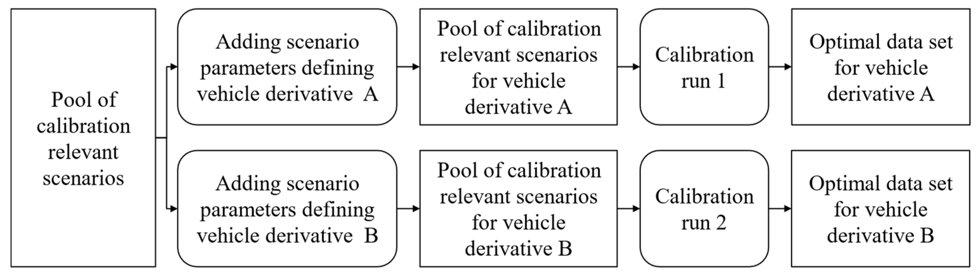
3.4. Use Case 4: Calibration for Different Vehicle Derivatives

The basic motivation for using data sets of calibration parameters is the possibility of deploying different systems, not only ADAS/ADS, in different vehicle derivatives without having separate software versions [26]. Different derivatives refer not only to vehicles featuring different configurations but also to different model series or even platforms on which an ADAS/ADS is deployed.

In order to generate data sets for different vehicle derivatives in virtual calibration, derivative-specific properties must be covered by the vehicle models used in the simulation. Additionally, these properties are stored as scenario parameters in the logical scenario database for each logical scenario to make them accessible for virtual calibration methods in the testing agent module. Derivative-specific properties may include, for example, differences in sensor positions but also the computation performance of partner systems. In each calibration run, calibration-relevant properties of the ego vehicle are defined within each logical scenario through scenario parameters.

Figure 6. Structure of virtual calibration method for different vehicle derivatives.

Figure 6. Structure of virtual calibration method for different vehicle derivatives.

As illustrated in Figure 6, the pool of calibration-relevant scenarios is enriched by scenario parameters defining the respective vehicle derivative. These are added to ${\mathit{s}\mathit{p}}_m$ and ${\mathit{S}\mathit{P}}_{\mathrm{v}\mathrm{a}\mathrm{l}\mathrm{u}\mathrm{e}\mathrm{s},m}$ for each logical scenario within $\mathit{l}\mathit{s}$. For each data set to be generated for an individual vehicle derivative, a calibration run has to be performed. The multi-scenario-level method of use case 1 can be applied if a large set of scenarios must be considered while keeping the same ego vehicle-relevant scenario parameters for each concrete scenario. In addition, different performance rating evaluation metrics and market-specific scenarios can be considered, as in use case 3, if some derivatives are only offered in certain markets.

3.5. Use Case 5: Calibration for Different Sub-Areas of the ODD

To optimize the behavior of ADAS/ADS, different data sets can be deployed for different sub-areas of the system’s ODD. The system switches to the corresponding data set if vehicle sensors indicate the vehicle is moving in the respective sub-area [27]. Sub-areas can be, for example, different road categories, weather conditions, or system settings by the driver. For example, using a different data set for traffic jams in an ACC can increase the naturalness of driving.

To generate data sets for different ODD sub-areas in virtual calibration, the entire pool of calibration-relevant scenarios of the system’s ODD is divided into sub-pools of scenarios for each sub-area of the ODD.

Figure 7. Structure of virtual calibration method for different ODDs.

Figure 7. Structure of virtual calibration method for different ODDs.

The division of scenarios can be performed using the scenario parameters of concrete scenarios defined through ${\mathit{s}\mathit{p}}_m$ and ${\mathit{S}\mathit{P}}_{\mathrm{v}\mathrm{a}\mathrm{l}\mathrm{u}\mathrm{e}\mathrm{s},m}$. For example, target cut-in scenarios featuring a velocity below 10 km/h can be assigned to traffic jam driving. The probability of the occurrence of concrete scenarios in real road traffic within ODD sub-areas can provide the necessary data to perform the division of the scenario pool. As illustrated in Figure 7, optimal data sets for each ODD sub-area are created by individual calibration runs that can apply the presented multi-scenario-level method if large scenario pools need to be considered.

4. Implementation and Evaluation

In this section, implementations of the presented methods for virtual ADAS/ADS calibration are demonstrated, and their results are evaluated. All implementations are executed on a personal computer featuring an Intel Core i7-9850H CPU, NVIDIA Quadro T2000 GPU, and 32 GB RAM. The focus is on the functionality of methods and not on validating simulation models, scenario models, or evaluation metrics, which are considered available. To create example use cases, a simplified model of an ACC controller is implemented as a SUT based on the sliding-mode principle, as presented by Liesner [10].

Figure 8. ACC controller implemented as example SUT.

Figure 8. ACC controller implemented as example SUT.

The illustrated ACC controller in Figure 8 receives as control inputs the velocity $v_{\mathrm{e}\mathrm{g}\mathrm{o}}\in \mathbb{R}$ of the ego vehicle, the acceleration $a_{\mathrm{e}\mathrm{g}\mathrm{o}}\in \mathbb{R}$, the distance $∆x\in \mathbb{R}$, and the velocity $v_{\mathrm{t}\mathrm{a}\mathrm{r}\mathrm{g}\mathrm{e}\mathrm{t}}\in \mathbb{R}$ of a recognized target vehicle in the driving corridor of the ego vehicle. Object perception is not part of the SUT but is implemented as a partner system in the ego vehicle model. Additional control inputs are a minimum offset distance ${∆x}_{\mathrm{O}\mathrm{f}\mathrm{f}\mathrm{s}\mathrm{e}\mathrm{t}}\in \mathbb{R}$ to other vehicles and a set velocity $v_{\mathrm{s}\mathrm{e}\mathrm{t}}\in \mathbb{R}$ and set a time gap ${\tau }_{\mathrm{s}\mathrm{e}\mathrm{t}}\in \mathbb{R}$ specified by the driver model. In function (I), a desired relative velocity change ${∆v}_{\mathrm{t}\mathrm{w}}\in \mathbb{R}$ is determined from the desired distance $∆x_{\mathrm{w}}\in \mathbb{R}$, actual distance $∆x\in \mathbb{R}$ and velocity signals when following another vehicle. Function (I) is formed by two horizontal parabolas and a straight line, according to Liesner [10], with ${∆v}_{\mathrm{t}\mathrm{w}}$ limited to prevent the total desired velocity from being higher than $v_{\mathrm{s}\mathrm{e}\mathrm{t}}$. In free driving, without a detected target vehicle, the desired velocity change ${∆v}_{\mathrm{w}}\in \mathbb{R}$ is determined from the difference between set velocity $v_{\mathrm{s}\mathrm{e}\mathrm{t}}$ and ego vehicle velocity $v_{\mathrm{s}\mathrm{e}\mathrm{t}}$. The desired acceleration $a_{\mathrm{w}}\in \mathbb{R}$ of the ego vehicle is calculated using the functions (II) for free driving and (III) for following a target vehicle. These are linear functions calculating $a_{\mathrm{w}}$ based on the total desired velocity change ${∆v}_{\mathrm{w}}$, using different gradients for positive ${∆v}_{\mathrm{w}}$ than for negative ${∆v}_{\mathrm{w}}$. Function (III) is characterized by two straight lines according to the following formula (5), with $m_{\mathrm{a},\mathrm{p}\mathrm{o}\mathrm{s},\mathrm{f}\mathrm{o}\mathrm{l}\mathrm{l}\mathrm{o}\mathrm{w}}\in \mathbb{R}$ and $m_{\mathrm{a},\mathrm{n}\mathrm{e}\mathrm{g},\mathrm{f}\mathrm{o}\mathrm{l}\mathrm{l}\mathrm{o}\mathrm{w}}\in \mathbb{R}$ being calibration parameters to modify the acceleration behavior of the ACC when following a target vehicle.

$$a_{\mathrm{w}}=\left\{\begin{array}{cc}{∆v}_{\mathrm{w}}·m_{\mathrm{a},\mathrm{p}\mathrm{o}\mathrm{s},\mathrm{f}\mathrm{o}\mathrm{l}\mathrm{l}\mathrm{o}\mathrm{w}}& {\mathrm{i}\mathrm{f}∆v}_{\mathrm{w}}\ge 0\\ {∆v}_{\mathrm{w}}·m_{\mathrm{a},\mathrm{n}\mathrm{e}\mathrm{g},\mathrm{f}\mathrm{o}\mathrm{l}\mathrm{l}\mathrm{o}\mathrm{w}}& {\mathrm{i}\mathrm{f}∆v}_{\mathrm{w}}<0\end{array}\right.$$

(5)

The selection of the outputs of functions (II) and (III) depends on detecting a target vehicle in the driving corridor in front of the ego vehicle, illustrated as a switch in Figure 8. Next follows the application of limits for ACC-controlled accelerations according to ISO 22179 [28]. In addition, a gradient limit $j_{\mathrm{l}\mathrm{i}\mathrm{m}\mathrm{i}\mathrm{t},\mathrm{f}\mathrm{r}\mathrm{e}\mathrm{e}}\in \mathbb{R}$ is applied for free driving and $j_{\mathrm{l}\mathrm{i}\mathrm{m}\mathrm{i}\mathrm{t},\mathrm{f}\mathrm{o}\mathrm{l}\mathrm{l}\mathrm{o}\mathrm{w}}\in \mathbb{R}$ for following a target vehicle, which are additional calibration parameters to modify the acceleration behavior of the SUT. In the final step, $a_{\mathrm{w}}$ is passed to a PI controller, which calculates a desired drive torque $M_{\mathrm{w}}\in \mathbb{R}$ which results in a throttle value ${\phi }_{\mathrm{t}\mathrm{h}\mathrm{r}\mathrm{o}\mathrm{t}\mathrm{t}\mathrm{l}\mathrm{e}}\in \left[\mathrm{0,1}\right]$ and a brake value ${\phi }_{\mathrm{b}\mathrm{r}\mathrm{a}\mathrm{k}\mathrm{e}}\in \left[\mathrm{0,1}\right]$.

The ACC model shown in Figure 8 represents a simplified implementation to demonstrate the methods presented in this paper. It features only a part of the functionalities of a series of ACCs but is suitable for demonstrating and evaluating example use cases and methods.

For virtual testing of the SUT, the open-source CARLA [29] simulation based on Unreal Game Engine is integrated into the simulation module of the virtual ADAS/ADS testing framework presented in Section 2. With the Scenario Runner add-on and the Metrics Manager add-on, different logical scenarios and performance evaluation metrics can be implemented. While the simulation of vehicle dynamics uses the already integrated NVIDIA PhysX model [30] in CARLA, sensors and perception systems are modeled by a delay $T_{\mathrm{p}\mathrm{e}\mathrm{r}\mathrm{c}\mathrm{e}\mathrm{p}\mathrm{t}\mathrm{i}\mathrm{o}\mathrm{n}}\in \mathbb{R}$ when detecting new vehicles in the driving corridor of the ego vehicle. The implementation also includes a driver model that applies a PI controller to take over lateral control of the ego vehicle and transfers $v_{\mathrm{s}\mathrm{e}\mathrm{t}}$ and ${\tau }_{\mathrm{s}\mathrm{e}\mathrm{t}}$ to set up the SUT.

4.1. Implementation and Evaluation of Multi-Scenario-Level Method for Use Case 1

The multi-scenario-level virtual calibration method introduced in Section 3.1 provides an approach to tackle the challenge of considering a large set of logical and concrete scenarios in ADAS/ADS calibration. In the following example, the method will be applied to calibrate the presented ACC model in different concrete target cut-in scenarios. In this logical scenario, the ego vehicle drives in a free lane until a target vehicle cuts into that lane in front of it. The ACC operates first in free driving mode and then changes to following the new target vehicle. The logical target cut-in scenario is implemented in the logical scenario database of the testing framework and features the following variable scenario parameters:

• Distance $d_{\mathrm{c}\mathrm{u}\mathrm{t}-\mathrm{i}\mathrm{n}}\in \mathbb{R}$ in m between the target vehicle and the ego vehicle when cut-in is performed by the target vehicle (driving environment cluster)
• Relative velocity $v_{\mathrm{r}\mathrm{e}\mathrm{l}}\in \mathbb{R}$ in km/h between target velocity and ego velocity during and after target cut-in (driving environment cluster)
• Lane change duration $T_{\mathrm{c}\mathrm{u}\mathrm{t}-\mathrm{i}\mathrm{n}}\in \mathbb{R}$ in s of the target vehicle (driving environment cluster)
• Desired velocity $v_{\mathrm{s}\mathrm{e}\mathrm{t}}$ in km/h set up by the driver (driver cluster)
• Desired time gap ${\tau }_{\mathrm{s}\mathrm{e}\mathrm{t}}$ in s set up by driver (driver cluster)
• Delay $T_{\mathrm{p}\mathrm{e}\mathrm{r}\mathrm{c}\mathrm{e}\mathrm{p}\mathrm{t}\mathrm{i}\mathrm{o}\mathrm{n}}$ in s of perception hardware and software of the ego vehicle (ego vehicle cluster)

Other characteristics of the logical scenario, such as the scenery of a three-lane straight highway, the powertrain and chassis of the ego vehicle, and parameters of lateral control by the driver model, are not implemented as variable scenario parameters in this example and remain constant.

The presented ACC model’s acceleration behavior when following another vehicle is controlled by calibration parameters $m_{\mathrm{a},\mathrm{p}\mathrm{o}\mathrm{s},\mathrm{f}\mathrm{o}\mathrm{l}\mathrm{l}\mathrm{o}\mathrm{w}}$, $m_{\mathrm{a},\mathrm{n}\mathrm{e}\mathrm{g},\mathrm{f}\mathrm{o}\mathrm{l}\mathrm{l}\mathrm{o}\mathrm{w}}$ and $j_{\mathrm{l}\mathrm{i}\mathrm{m}\mathrm{i}\mathrm{t},\mathrm{f}\mathrm{o}\mathrm{l}\mathrm{l}\mathrm{o}\mathrm{w}}$. In the example use case, these parameters are optimized in nine concrete target cut-in scenarios, which are detailed in

Table A1. Concrete target cut-in scenarios to be considered in the example use case.

Concrete Scenario Description	${\mathit{d}}_{\mathbf{c}\mathbf{u}\mathbf{t}-\mathbf{i}\mathbf{n}}$	${\mathit{v}}_{\mathbf{r}\mathbf{e}\mathbf{l}}$	${\mathit{T}}_{\mathbf{c}\mathbf{u}\mathbf{t}-\mathbf{i}\mathbf{n}}$	${\mathit{v}}_{\mathbf{s}\mathbf{e}\mathbf{t}}$	${\mathit{\tau }}_{\mathbf{s}\mathbf{e}\mathbf{t}}$	${\mathit{T}}_{\mathbf{p}\mathbf{e}\mathbf{r}\mathbf{c}\mathbf{e}\mathbf{p}\mathbf{t}\mathbf{i}\mathbf{o}\mathbf{n}}$
Representative country road scenario	40	−10	4	100	2.5	0.1
Representative city scenario	20	−5	4	50	2.5	0.1
Representative highway scenario	60	−20	4	140	2.5	0.1
Additional country road scenario	30	−5	4	100	2.5	0.1
Additional city scenario	15	−2	4	50	2.5	0.1
Additional highway scenario	50	−5	4	140	2.5	0.1
Challenging country road scenario	30	−20	4	100	2.5	0.1
Challenging city scenario	15	−10	4	50	2.5	0.1
Challenging highway scenario	50	−30	4	140	2.5	0.1

in Appendix A. Other calibration parameters are kept constant. The parameter $m_{\mathrm{a},\mathrm{p}\mathrm{o}\mathrm{s},\mathrm{f}\mathrm{o}\mathrm{l}\mathrm{l}\mathrm{o}\mathrm{w}}$ has only a small effect in the considered target cut-in scenario but is nevertheless included in optimization to show the robustness of the method against slightly influential parameters. The scenario pool shown in Table A1 was assembled manually in this example. In an extended application, the scenarios to be considered for calibration can be derived from real driving data or expert knowledge. For performance evaluation, a metric based on quality loss functions is implemented in the evaluation database of the testing framework, which is explained in more detail in Section 4.2. The metric assesses the performance of the ACC model in the considered target cut-in scenario by an index from 1 to 10.

In the scenario pool of Level 1, only three representative concrete target cut-in scenarios for three road categories, country road, city, and highway, are present. Co-domains of calibration parameters are limited to $m_{\mathrm{a},\mathrm{p}\mathrm{o}\mathrm{s},\mathrm{f}\mathrm{o}\mathrm{l}\mathrm{l}\mathrm{o}\mathrm{w}}\in \left[\mathrm{0.1,1}\right]$, $m_{\mathrm{a},\mathrm{n}\mathrm{e}\mathrm{g},\mathrm{f}\mathrm{o}\mathrm{l}\mathrm{l}\mathrm{o}\mathrm{w}}\in \left[\mathrm{0.1,1}\right]$ and $j_{\mathrm{l}\mathrm{i}\mathrm{m}\mathrm{i}\mathrm{t},\mathrm{f}\mathrm{o}\mathrm{l}\mathrm{l}\mathrm{o}\mathrm{w}}\in \left[\mathrm{0.5,6}\right]$. Optimization is performed using the presented PSO, which is implemented in the testing agent strategy module of the framework. It is configured with $\mathcal{X}=0.4,a_1=0.4$, $a_2=0.6,n_{\mathrm{p}\mathrm{a}\mathrm{r}\mathrm{t}\mathrm{i}\mathrm{c}\mathrm{l}\mathrm{e}\mathrm{s}}=20$ and $n_{\mathrm{i}\mathrm{t}\mathrm{e}\mathrm{r}\mathrm{a}\mathrm{t}\mathrm{i}\mathrm{o}\mathrm{n}\mathrm{s}}=30$.

Figure 9. Optimization in Level 1.

Figure 9. Optimization in Level 1.

Besides inputs and outputs of optimization in Level 1, Figure 9 shows costs in each iteration in the upper plot and evaluated particle positions in the lower plot. Large points in the lower plot mark initial particle positions, chosen randomly during PSO initialization in this first optimization level. PSO converges to the optimal position $m_{\mathrm{a},\mathrm{p}\mathrm{o}\mathrm{s},\mathrm{f}\mathrm{o}\mathrm{l}\mathrm{l}\mathrm{o}\mathrm{w}}=0.56$, $m_{\mathrm{a},\mathrm{n}\mathrm{e}\mathrm{g},\mathrm{f}\mathrm{o}\mathrm{l}\mathrm{l}\mathrm{o}\mathrm{w}}=0.24$ and $j_{\mathrm{l}\mathrm{i}\mathrm{m}\mathrm{i}\mathrm{t},\mathrm{f}\mathrm{o}\mathrm{l}\mathrm{l}\mathrm{o}\mathrm{w}}=0.74$ with cost $y_{\mathrm{b}\mathrm{e}\mathrm{s}\mathrm{t}}=0.77$ and the associated performance rating of $9.23$ on an index from 1 to 10. The worst position analyzed in this optimization run has a performance rating of $5.79$. Of the theoretically 1800 test cases to be processed according to formula (2), only 786 were needed due to the reuse of already processed particle positions presented in Section 2.

The identified optimal position is used to calculate initial particle positions for level 2, in which all nine concrete target cut-in scenarios of Table A1 are considered for calibration. In addition to the representative concrete scenarios considered in Level 1, an additional scenario and a challenging scenario are added for each road category. The shift matrix ${\mathit{X}}_{\mathrm{s}\mathrm{h}\mathrm{i}\mathrm{f}\mathrm{t}}$ in formula (3) is chosen as follows based on the topology presented in formula (4):

$${\mathit{X}}_{\mathrm{s}\mathrm{h}\mathrm{i}\mathrm{f}\mathrm{t}}=\left(\begin{array}{ccccccc}0& -0.2& 0.2& 0& 0& 0& 0\\ 0& 0& 0& -1.4& 0.2& 0& 0\\ 0& 0& 0& 0& 0& -0.24& 0.5\end{array}\right)$$

(6)

In (6), the values for decreasing and increasing individual calibration parameters are not the same as in (4) for $m_{\mathrm{a},\mathrm{n}\mathrm{e}\mathrm{g},\mathrm{f}\mathrm{o}\mathrm{l}\mathrm{l}\mathrm{o}\mathrm{w}}$ and $j_{\mathrm{l}\mathrm{i}\mathrm{m}\mathrm{i}\mathrm{t},\mathrm{f}\mathrm{o}\mathrm{l}\mathrm{l}\mathrm{o}\mathrm{w}}$, since otherwise their co-domains would be violated. Therefore, the following optimization in Level 2 is performed using a lower number of particles and a lower number of iterations than in Level 1.

Figure 10. Optimization in Level 2.

Figure 10. Optimization in Level 2.

Figure 10 illustrates that PSO converges to an optimal position, similar to Level 1. Considering all concrete scenarios in Table A1, $m_{\mathrm{a},\mathrm{p}\mathrm{o}\mathrm{s},\mathrm{f}\mathrm{o}\mathrm{l}\mathrm{l}\mathrm{o}\mathrm{w}}=0.2$, $m_{\mathrm{a},\mathrm{n}\mathrm{e}\mathrm{g},\mathrm{f}\mathrm{o}\mathrm{l}\mathrm{l}\mathrm{o}\mathrm{w}}=0.31$ and $j_{\mathrm{l}\mathrm{i}\mathrm{m}\mathrm{i}\mathrm{t},\mathrm{f}\mathrm{o}\mathrm{l}\mathrm{l}\mathrm{o}\mathrm{w}}=0.69$ are identified as the optimal data set with a performance rating of $8.87$. While the optimal values of $m_{\mathrm{a},\mathrm{n}\mathrm{e}\mathrm{g},\mathrm{f}\mathrm{o}\mathrm{l}\mathrm{l}\mathrm{o}\mathrm{w}}$ and $j_{\mathrm{l}\mathrm{i}\mathrm{m}\mathrm{i}\mathrm{t},\mathrm{f}\mathrm{o}\mathrm{l}\mathrm{l}\mathrm{o}\mathrm{w}}$ are not far from the optimal values of Level 1 and within the initial positions defined by ${\mathit{C}\mathit{P}}_{\mathrm{v}\mathrm{a}\mathrm{r}\mathrm{y},\mathrm{i}\mathrm{n}\mathrm{i}\mathrm{t}}$, the optimal value of $m_{\mathrm{a},\mathrm{p}\mathrm{o}\mathrm{s},\mathrm{f}\mathrm{o}\mathrm{l}\mathrm{l}\mathrm{o}\mathrm{w}}$ in Level 2 differs strongly from Level 1. This is due to the small effect of this calibration parameter on the performance of the SUT in the target cut-in scenario. If other logical scenarios, such as target acceleration or target cut-out behind a new target, were considered in optimization, similar behavior to that for the other parameters would also occur for this calibration parameter. Nevertheless, the method shows robustness to parameters with little effect in the scenarios considered since optimal values are identified for $m_{\mathrm{a},\mathrm{n}\mathrm{e}\mathrm{g},\mathrm{f}\mathrm{o}\mathrm{l}\mathrm{l}\mathrm{o}\mathrm{w}}$ and $j_{\mathrm{l}\mathrm{i}\mathrm{m}\mathrm{i}\mathrm{t},\mathrm{f}\mathrm{o}\mathrm{l}\mathrm{l}\mathrm{o}\mathrm{w}}$.

This example use case shows that with a suitable choice of representative scenarios in Level 1 and a suitable topology for initial particle positions in Level 2 defined by ${\mathit{X}}_{\mathrm{s}\mathrm{h}\mathrm{i}\mathrm{f}\mathrm{t}}$, an optimal data set in Level 2 can be identified using fewer PSO particles and iterations. The question of how to distribute logical and concrete scenarios to different levels and which topologies for ${\mathit{X}}_{\mathrm{s}\mathrm{h}\mathrm{i}\mathrm{f}\mathrm{t}}$ result in a beneficial performance of the method is the subject of subsequent research.

Besides the identification of an optimal data set for an overall optimal performance rating, the method also allows for checking in which of the concrete scenarios the identified data set has weaknesses. In this example, the lowest performance rating of individual concrete scenarios is present for the challenging highway scenario, with a performance rating of $8.01$. If necessary, this information can be used to define specific software changes to improve ACC behavior in this scenario. Due to the reuse of already evaluated particle positions, only 657 test cases instead of 945 test cases had to be processed in this optimization run.

To quantify the potential of the multi-scenario-level method, the optimization of the three calibration parameters is additionally performed at only one level, featuring all concrete scenarios at once with random initial particle positions. Figure 11 shows results of this calibration run.

Figure 11. Optimization without multi-scenario-level method.

Figure 11. Optimization without multi-scenario-level method.

It can be observed that the optimal values of $m_{\mathrm{a},\mathrm{n}\mathrm{e}\mathrm{g},\mathrm{f}\mathrm{o}\mathrm{l}\mathrm{l}\mathrm{o}\mathrm{w}}$ and $j_{\mathrm{l}\mathrm{i}\mathrm{m}\mathrm{i}\mathrm{t},\mathrm{f}\mathrm{o}\mathrm{l}\mathrm{l}\mathrm{o}\mathrm{w}}$ as well as the cost $y_{\mathrm{b}\mathrm{e}\mathrm{s}\mathrm{t}}$ of optimal position are close to the values of Figure 10. The small deviation can be explained by the non-deterministic behavior of PSO and simulation. The calibration parameter $m_{\mathrm{a},\mathrm{p}\mathrm{o}\mathrm{s},\mathrm{f}\mathrm{o}\mathrm{l}\mathrm{l}\mathrm{o}\mathrm{w}}$ deviates strongly since it has little effect on the performance of the SUT in this logical scenario.

Using the multi-scenario-level method for virtual calibration of the ACC in this example use case reduced the number of test cases required to 1443. This represents a significant decrease compared to the 2349 test cases required for normal optimization. Thus, the efficiency of virtual calibration, measured in test cases to be processed, was increased by 38.57% using the multi-scenario-level method. It can be assumed that this increase in efficiency is even higher if a larger pool of logical and concrete scenarios is considered. The processing time of test cases in this implementation, including initialization and evaluation, is 1.5 min. Test cases are performed in real-time as it is required for hardware-in-the-loop (HiL) testing. In this simple example use case, the multi-scenario-level method saved 22.65 h of simulation time. Efficiency could be further increased by distributing test cases among a cluster of HiL test benches, for which the PSO is well suited due to the possibility of parallel particle position evaluation.

4.2. Implementation and Evaluation of Different Performance Rating Metrics for Use Cases 2 and 3

To calibrate ADAS/ADS for different system modes and markets, corresponding methods are presented in Section 3.2 and Section 3.3 of this paper. In the following example implementation, the use case is to identify an optimal data set for comfort-oriented ACC behavior and a safety-oriented data set in the already introduced target cut-in scenario. The comfort-oriented data set does not neglect safety but allows the ego vehicle to drive closer to target vehicles in favor of more comfortable braking. The safety-oriented data set can be applied in specific markets where customers value the safer behavior of the ACC over comfort. A core component of methods to cover this use case is different performance rating metrics, which are used to calculate costs for optimization of the two required data sets. In this example implementation, performance evaluation metrics were defined based on expert knowledge rather than extensive subject studies. Implemented metrics in the evaluation database of the testing framework are based on quality loss functions introduced by Taguchi et al. [31], which are used to map direct physical KPIs to an overall performance rating. For the logical target cut-in scenario, the following direct KPIs are defined in the evaluation database of the framework:

• Mean longitudinal braking deceleration ${\bar{a}}_{\mathrm{b}\mathrm{r}\mathrm{a}\mathrm{k}\mathrm{e}}\in \mathbb{R}$ in $\mathrm{m}/{\mathrm{s}}^2$ of ego vehicle during cut-in
• Maximal longitudinal braking deceleration $a_{\mathrm{b}\mathrm{r}\mathrm{a}\mathrm{k}\mathrm{e},\mathrm{m}\mathrm{a}\mathrm{x}}\in \mathbb{R}$ in $\mathrm{m}/{\mathrm{s}}^2$ of ego vehicle during cut-in
• Minimal longitudinal jerk $j_{\mathrm{m}\mathrm{i}\mathrm{n}}\in \mathbb{R}$ in $\mathrm{m}/{\mathrm{s}}^3$ of ego vehicle during cut-in
• Maximal longitudinal jerk $j_{\mathrm{m}\mathrm{a}\mathrm{x}}\in \mathbb{R}$ in $\mathrm{m}/{\mathrm{s}}^3$ of ego vehicle during cut-in
• Minimal time to collision $TT{C}_{\mathrm{m}\mathrm{i}\mathrm{n}}\in \mathbb{R}$ in s between ego vehicle and target vehicle during cut-in ($TTC=d/v_{\mathrm{r}\mathrm{e}\mathrm{l}}$ with $d\in \mathbb{R}$ being the distance and $v_{\mathrm{r}\mathrm{e}\mathrm{l}}\in \mathbb{R}$ being the relative velocity between the two vehicles)
• Risk time $T_{\mathrm{r}\mathrm{i}\mathrm{s}\mathrm{k}}\in \mathbb{R}$ in s, which is the duration of the ego vehicle violating the legislative minimum distance to the target vehicle
• Velocity immersion $v_{\mathrm{i}\mathrm{m}\mathrm{m}\mathrm{e}\mathrm{r}\mathrm{s}\mathrm{i}\mathrm{o}\mathrm{n}}\in \mathbb{R}$ in $\mathrm{m}/\mathrm{s}$, which is the relative velocity at which the ego vehicle immerses below the velocity of the target vehicle during braking
• Minimal time gap ${\tau }_{\mathrm{m}\mathrm{i}\mathrm{n}}\in \mathbb{R}$ in s between ego vehicle and target vehicle during cut-in ($\tau =d/v_{\mathrm{e}\mathrm{g}\mathrm{o}}$ with $d\in \mathbb{R}$ being the distance between the two vehicles and $v_{\mathrm{e}\mathrm{g}\mathrm{o}}\in \mathbb{R}$ being the velocity of the ego vehicle)

Quality loss functions are implemented as indirect KPIs in the evaluation database to calculate costs, which map direct KPIs to indices from 1 to 10 to derive an overall performance rating. These indices are used to calculate mean ratings for the individual performance rating aspects of comfort, safety, and naturalness of driving, which are weighted, and a mean value for the overall performance rating is calculated.

Two different performance rating metrics are implemented as indirect KPIs to identify the two different data sets during calibration. Appendix B includes

Table A2. Overview of comfort-oriented performance rating metric.

Performance Rating Aspect	Direct KPI	Quality Loss Function	Parameters of Quality Loss Function	Performance Rating Aspect Weight
Comfort	${\bar{a}}_{\mathrm{b}\mathrm{r}\mathrm{a}\mathrm{k}\mathrm{e}}$	Asymmetric target value	$m=1,A_0=1,{∆}_0=4,$ $A_1=0,{∆}_1=1$	4
	$a_{\mathrm{b}\mathrm{r}\mathrm{a}\mathrm{k}\mathrm{e},\mathrm{m}\mathrm{a}\mathrm{x}}$	Asymmetric target value	$m=1.5,A_0=1,{∆}_0=4,$ $A_1=0,{∆}_1=1$
	$j_{\mathrm{m}\mathrm{i}\mathrm{n}}$	Minimizing	$A_0=6,{∆}_0=2$
	$j_{\mathrm{m}\mathrm{a}\mathrm{x}}$	Minimizing	$A_0=6,{∆}_0=2$
Safety	$TT{C}_{\mathrm{m}\mathrm{i}\mathrm{n}}$	Asymmetric target value	$m=8,A_0=0,{∆}_0=1,$ $A_1=2,{∆}_1=6$	2
	$T_{\mathrm{r}\mathrm{i}\mathrm{s}\mathrm{k}}$	Asymmetric target value	$m=10,A_0=4,{∆}_0=6,$ $A_1=0,{∆}_1=1$
Naturalness of driving	$v_{\mathrm{i}\mathrm{m}\mathrm{m}\mathrm{e}\mathrm{r}\mathrm{s}\mathrm{i}\mathrm{o}\mathrm{n}}$	Asymmetric target value	$m=2.22,A_0=4,{∆}_0=0.56,$ $A_1=0,{∆}_1=1$	1
	${\tau }_{\mathrm{m}\mathrm{i}\mathrm{n}}$	Asymmetric target value	$m=1.5,A_0=2,{∆}_0=1,$ $A_1=8,{∆}_1=1$

showing all values of the performance rating metric to calculate costs for optimization of the comfort-oriented data set.

Table A3. Overview of safety-oriented performance rating metric.

Performance Rating Aspect	Direct KPI	Quality Loss Function	Parameters of Quality Loss Function	Performance Rating Aspect Weight
Comfort	${\bar{a}}_{\mathrm{b}\mathrm{r}\mathrm{a}\mathrm{k}\mathrm{e}}$	Asymmetric target value	$m=1,A_0=1,{∆}_0=4,$ $A_1=0,{∆}_1=1$	1
	$a_{\mathrm{b}\mathrm{r}\mathrm{a}\mathrm{k}\mathrm{e},\mathrm{m}\mathrm{a}\mathrm{x}}$	Asymmetric target value	$m=1.5,A_0=1,{∆}_0=4,$ $A_1=0,{∆}_1=1$
	$j_{\mathrm{m}\mathrm{i}\mathrm{n}}$	Minimizing	$A_0=6,{∆}_0=2$
	$j_{\mathrm{m}\mathrm{a}\mathrm{x}}$	Minimizing	$A_0=6,{∆}_0=2$
Safety	$TT{C}_{\mathrm{m}\mathrm{i}\mathrm{n}}$	Asymmetric target value	$m=8,A_0=0,{∆}_0=1,$ $A_1=4,{∆}_1=2$	2
	$T_{\mathrm{r}\mathrm{i}\mathrm{s}\mathrm{k}}$	Asymmetric target value	$m=4,A_0=4,{∆}_0=4,$ $A_1=0,{∆}_1=1$
Naturalness of driving	$v_{\mathrm{i}\mathrm{m}\mathrm{m}\mathrm{e}\mathrm{r}\mathrm{s}\mathrm{i}\mathrm{o}\mathrm{n}}$	Asymmetric target value	$m=2.22,A_0=4,{∆}_0=0.56,$ $A_1=0,{∆}_1=1$	1
	${\tau }_{\mathrm{m}\mathrm{i}\mathrm{n}}$	Asymmetric target value	$m=1.5,A_0=2,{∆}_0=1,$ $A_1=8,{∆}_1=1$

shows the values of the safety-oriented performance rating metrics, while formulas (A1) and (A2) represent applied quality loss functions. There are differences implemented in the weights of individual performance rating aspects and in the definition of quality loss functions to map safety-relevant direct KPIs $TT{C}_{\mathrm{m}\mathrm{i}\mathrm{n}}$ and $T_{\mathrm{r}\mathrm{i}\mathrm{s}\mathrm{k}}$. The safety-oriented performance rating metric assigns more cost to lower $TT{C}_{\mathrm{m}\mathrm{i}\mathrm{n}}$ and higher $T_{\mathrm{r}\mathrm{i}\mathrm{s}\mathrm{k}}$, and weights the aspect rating for safety higher than for comfort.

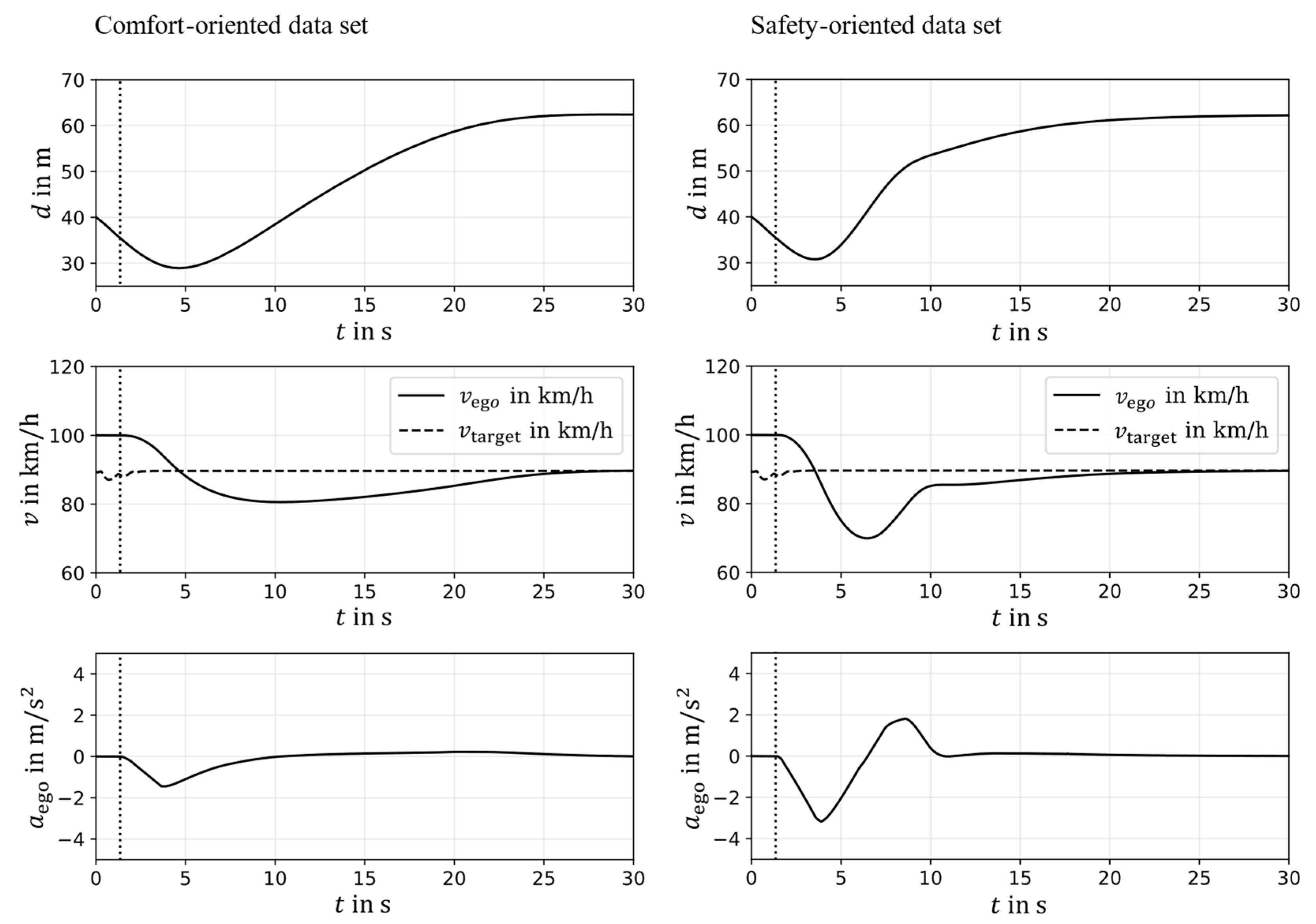
The optimization is performed using PSO, whereby the different performance rating metrics are applied to calculate costs. Since Section 4.1 already illustrated optimization for different concrete scenarios, this example focuses on evaluating different performance rating metrics. It only considers the representative country road target cut-in scenario of Table A1 during calibration. Optimization results in an optimal comfort-oriented data set with $m_{\mathrm{a},\mathrm{p}\mathrm{o}\mathrm{s},\mathrm{f}\mathrm{o}\mathrm{l}\mathrm{l}\mathrm{o}\mathrm{w}}=0.12$, $m_{\mathrm{a},\mathrm{n}\mathrm{e}\mathrm{g},\mathrm{f}\mathrm{o}\mathrm{l}\mathrm{l}\mathrm{o}\mathrm{w}}=0.17$ and $j_{\mathrm{l}\mathrm{i}\mathrm{m}\mathrm{i}\mathrm{t},\mathrm{f}\mathrm{o}\mathrm{l}\mathrm{l}\mathrm{o}\mathrm{w}}=0.73$ and a safety-oriented data set with $m_{\mathrm{a},\mathrm{p}\mathrm{o}\mathrm{s},\mathrm{f}\mathrm{o}\mathrm{l}\mathrm{l}\mathrm{o}\mathrm{w}}=0.49$, $m_{\mathrm{a},\mathrm{n}\mathrm{e}\mathrm{g},\mathrm{f}\mathrm{o}\mathrm{l}\mathrm{l}\mathrm{o}\mathrm{w}}=0.75$ and $j_{\mathrm{l}\mathrm{i}\mathrm{m}\mathrm{i}\mathrm{t},\mathrm{f}\mathrm{o}\mathrm{l}\mathrm{l}\mathrm{o}\mathrm{w}}=1.58$.

Figure 12. ACC behavior applies different optimal data sets for different markets.

Figure 12. ACC behavior applies different optimal data sets for different markets.

Figure 12 shows ACC behavior in the representative country road target cut-in scenario, applying the different data sets generated in calibration. Distance $d$ between vehicles, velocities of the ego and target vehicles, and acceleration $a_{\mathrm{e}\mathrm{g}\mathrm{o}}$ of the ego vehicle are shown. The vertical dotted line shows the point in time when the target vehicle crosses the dividing line between lanes. It can be observed that the implementation of different performance rating metrics successfully covered the example use case. Due to the calibrated parameters of the safety-oriented data set, the ACC model in the right plots allows for higher deceleration and jerk. Although the minimum distance between vehicles can only be changed slightly due to limitations of the implemented ACC model, a higher and “safer” distance to the target vehicle is established more quickly than when using the comfort-oriented data set.

The quality of data sets generated in virtual calibration can be improved by applying performance evaluation metrics featuring non-constant quality loss functions. Higher decelerations and jerks can be accepted for more challenging scenarios than for normal, unchallenging scenarios. This requirement can be covered by performance evaluation metrics featuring variable values of quality loss functions depending on scenario parameters. Since the focus of this paper is on virtual calibration methods, this is an objective for subsequent research.

4.3. Implementation and Evaluation of Different Vehicle Models for Use Case 4

Section 3.4 presents a method to calibrate ADAS/ADS for application in different vehicle derivatives. The core of the method is to implement derivative-specific properties in vehicle models in simulation and to make them accessible as scenario parameters stored in the logical scenario database of the framework. In the implemented example use case, the presented ACC has to be calibrated for two vehicle derivatives equipped with different perception systems to identify target vehicles in the driving corridor in front of the ego vehicle. Vehicle derivative A is equipped with an advanced perception system that includes extended sensors or neural networks trained with a larger dataset for target vehicle recognition. These properties can be considered by the scenario parameter $T_{\mathrm{p}\mathrm{e}\mathrm{r}\mathrm{c}\mathrm{e}\mathrm{p}\mathrm{t}\mathrm{i}\mathrm{o}\mathrm{n}}$ already presented in Section 4.1. The vehicle derivative equipped with an advanced perception system is assigned $T_{\mathrm{p}\mathrm{e}\mathrm{r}\mathrm{c}\mathrm{e}\mathrm{p}\mathrm{t}\mathrm{i}\mathrm{o}\mathrm{n}}=0.1$ in ${\mathit{S}\mathit{P}}_{\mathrm{v}\mathrm{a}\mathrm{l}\mathrm{u}\mathrm{e}\mathrm{s},1}$, while $T_{\mathrm{p}\mathrm{e}\mathrm{r}\mathrm{c}\mathrm{e}\mathrm{p}\mathrm{t}\mathrm{i}\mathrm{o}\mathrm{n}}=1$ is assigned to vehicle derivative B, which features a normal perception system.

Two optimization runs have to be performed to calibrate the ACC for each vehicle derivative. The concrete scenarios to be considered have to be enriched with the matching values of $T_{\mathrm{p}\mathrm{e}\mathrm{r}\mathrm{c}\mathrm{e}\mathrm{p}\mathrm{t}\mathrm{i}\mathrm{o}\mathrm{n}}$. As calibration for a large set of scenarios was already illustrated before, in this example use case only the representative country road target cut-in scenario of Table A1 is considered. The comfort-oriented performance rating metrics defined in Table A2 are used for cost calculation. Optimization results in an optimal data set $m_{\mathrm{a},\mathrm{p}\mathrm{o}\mathrm{s},\mathrm{f}\mathrm{o}\mathrm{l}\mathrm{l}\mathrm{o}\mathrm{w}}=0.12$, $m_{\mathrm{a},\mathrm{n}\mathrm{e}\mathrm{g},\mathrm{f}\mathrm{o}\mathrm{l}\mathrm{l}\mathrm{o}\mathrm{w}}=0.17$ and $j_{\mathrm{l}\mathrm{i}\mathrm{m}\mathrm{i}\mathrm{t},\mathrm{f}\mathrm{o}\mathrm{l}\mathrm{l}\mathrm{o}\mathrm{w}}=0.73$ for vehicle derivative A and $m_{\mathrm{a},\mathrm{p}\mathrm{o}\mathrm{s},\mathrm{f}\mathrm{o}\mathrm{l}\mathrm{l}\mathrm{o}\mathrm{w}}=0.3$, $m_{\mathrm{a},\mathrm{n}\mathrm{e}\mathrm{g},\mathrm{f}\mathrm{o}\mathrm{l}\mathrm{l}\mathrm{o}\mathrm{w}}=0.17$ and $j_{\mathrm{l}\mathrm{i}\mathrm{m}\mathrm{i}\mathrm{t},\mathrm{f}\mathrm{o}\mathrm{l}\mathrm{l}\mathrm{o}\mathrm{w}}=0.97$ for vehicle derivative B. During calibration of the ACC in vehicle derivative A, an optimal performance rating of $9.6$ is achieved, while in vehicle derivative B, a performance rating of $9.29$ is achieved. The following Figure 13 shows the behavior of the ACC in the different vehicle derivates after applying the individual optimal data sets.

Figure 13. ACC behavior when applying different optimal data sets for different vehicle derivatives.

Figure 13. ACC behavior when applying different optimal data sets for different vehicle derivatives.

The effects of the enhanced perception system can be observed in the reaction of the ACC to the target vehicle crossing the lane boundary of the ego-lane. This is shown by a dotted vertical line in Figure 13. Vehicle derivative B experiences a long delay in detecting the new target vehicle, leading to later braking by the ACC than in vehicle derivative A. Therefore, the optimal data set generated for vehicle derivative B in virtual calibration features a higher value for $j_{\mathrm{l}\mathrm{i}\mathrm{m}\mathrm{i}\mathrm{t},\mathrm{f}\mathrm{o}\mathrm{l}\mathrm{l}\mathrm{o}\mathrm{w}}$, which allows a higher braking jerk. This prevents the ego vehicle from driving too close to the target vehicle for too long. Nevertheless, the ACC does not perform as well as in vehicle derivative A, as can be observed from different performance ratings. This demonstrates that ADAS/ADS calibration also reaches limits where hardware or software modifications are necessary to improve system performance.

4.4. Implementation and Evaluation of Division of Scenarios in ODD Sub-Areas for Use Case 5

In Section 3.5, a method is presented to generate different data sets for different sub-areas of the ODD in virtual ADAS/ADS calibration. As an example of implementation, the already introduced concrete target cut-in scenarios in Table A1 are divided into sub-areas according to the road category. This results in three pools of calibration-relevant scenarios for three road categories. After optimization with the PSO and the comfort-oriented performance rating metric of Table A2, the following optimal data sets are generated:

Table 1. Optimal data sets and costs for different ODD sub-areas.

	Country Road	City	Highway
$m_{\mathrm{a},\mathrm{p}\mathrm{o}\mathrm{s},\mathrm{f}\mathrm{o}\mathrm{l}\mathrm{l}\mathrm{o}\mathrm{w}}$	0.15	0.46	0.51
$m_{\mathrm{a},\mathrm{n}\mathrm{e}\mathrm{g},\mathrm{f}\mathrm{o}\mathrm{l}\mathrm{l}\mathrm{o}\mathrm{w}}$	0.36	0.15	0.33
$j_{\mathrm{l}\mathrm{i}\mathrm{m}\mathrm{i}\mathrm{t},\mathrm{f}\mathrm{o}\mathrm{l}\mathrm{l}\mathrm{o}\mathrm{w}}$	0.7	0.61	0.72
$y_{\mathrm{b}\mathrm{e}\mathrm{s}\mathrm{t}}$	1.27	0.42	1.41

Table 1. Optimal data sets and costs for different ODD sub-areas.

	Country Road	City	Highway
$m_{\mathrm{a},\mathrm{p}\mathrm{o}\mathrm{s},\mathrm{f}\mathrm{o}\mathrm{l}\mathrm{l}\mathrm{o}\mathrm{w}}$	0.15	0.46	0.51
$m_{\mathrm{a},\mathrm{n}\mathrm{e}\mathrm{g},\mathrm{f}\mathrm{o}\mathrm{l}\mathrm{l}\mathrm{o}\mathrm{w}}$	0.36	0.15	0.33
$j_{\mathrm{l}\mathrm{i}\mathrm{m}\mathrm{i}\mathrm{t},\mathrm{f}\mathrm{o}\mathrm{l}\mathrm{l}\mathrm{o}\mathrm{w}}$	0.7	0.61	0.72
$y_{\mathrm{b}\mathrm{e}\mathrm{s}\mathrm{t}}$	1.27	0.42	1.41

Based on the optimal data sets and costs in Table 1, it can be observed that better performance ratings are achieved in city target cut-in scenarios due to lower velocities. However, a different data set of the ACC is useful in this sub-area of the ODD, while the values of calibration parameters for country road and highway scenarios are similar. The values of $m_{\mathrm{a},\mathrm{p}\mathrm{o}\mathrm{s},\mathrm{f}\mathrm{o}\mathrm{l}\mathrm{l}\mathrm{o}\mathrm{w}}$ do not align with those of other examples, as they have a minor impact on the target cut-in scenarios considered during calibration. Thus, two data sets can be generated by virtual calibration. One of the generated data sets is for city driving, and one is for country roads and highways. The system can identify the respective road category using map data or traffic sign recognition and switch between data sets to feature optimized behavior.

5. Conclusions and Future Work

This paper presents a holistic overview of the use cases of virtual ADAS/ADS calibration and methods to cover these use cases. A logical scenario database, an evaluation database featuring different performance rating metrics, and a particle swarm optimizer for test case sampling are core components of the presented methods. The discussed use cases involve the virtual calibration of ADAS/ADS in a variety of calibration-relevant scenarios for different system modes, customer groups, markets, vehicle derivatives, and sub-areas of their ODD. A multi-scenario-level calibration method is presented to tackle the challenge of a sharp increase in the number of test cases when considering a large set of calibration-relevant scenarios. This method is applied to optimize data sets iteratively for optimal system behavior in a variety of scenarios. In the implemented example, the efficiency of the virtual calibration of an ACC model can be increased by 38.57%, measured by the number of test cases to be simulated. In addition, it is illustrated how the ACC model can be virtually calibrated for comfort- and safety-oriented behavior by applying different performance rating metrics. By implementing different vehicle models in simulation, the ACC model can be calibrated for optimal behavior in a vehicle derivative featuring an enhanced perception system and for a derivative with a normal perception system. Finally, different data sets were generated for the road categories country road, city road, and highway, enabling the ACC to feature specific behavior for these sub-areas of its ODD. By applying the presented methods, data sets can efficiently be generated in virtual calibration in various use cases and serve as a starting point for fine-tuning in prototype vehicles.

In the next step, the presented methods can be tested and evaluated in combination with validated and enhanced simulation, scenario models, and performance rating metrics to calibrate a series of ADAS/ADS. This allows the evaluation of presented methods under more complex conditions and enables testing generated data sets in prototype vehicles. Advanced challenges can be investigated, such as the need for computational simulation performance in combination with hardware-in-the-loop test benches and the necessary simulation accuracy. In addition, the question of which logical and concrete scenarios to consider for calibration and at what level of the presented multi-scenario-level calibration method these scenarios should be placed has not yet been discussed. Data from real test drives featuring occurrence numbers of concrete scenarios can serve as input for approaches to answering this question.

References

- SAE International. J3016_202104—Taxonomy and Definitions for Terms Related to Driving Automation Systems for On-Road Motor Vehicles; SAE International: Warrendale, PA, USA, 2021. [Google Scholar] [CrossRef]
- Hakuli, S.; Krug, M. Virtuelle Integration. In Handbuch Fahrerassistenzsysteme; Springer Vieweg: Wiesbaden, Germany, 2015; pp. 125–138. ISBN 978-3-558-05733-5. [Google Scholar]
- PAS 1883:2020; Operational Design Domain (ODD) Taxonomy for an Automated Driving System (ADS)—Specification. The British Standards Institution: London, UK, 2020; ISBN 978-0-539-06735-4.
- Ulbrich, S.; Menzel, T.; Raschka, A.; Schuldt, F.; Maurer, M. Definition der Begriffe Szene, Situation und Szenario für das Automatisierte Fahren. In Fahrerassistenzworkshop; Walting, Germany, 2015. [Google Scholar]
- ISO 21448:2022-06; Road Vehicles—Safety of the Intended Functionality. ISO: Geneva, Switzerland, 2022.
- Wilhelm, U.; Ebel, S.; Weitzel, A. Funktionale Sicherheit und ISO 26262—Validierung von Systemen mit funktionaler Unzulänglichkeit. In Handbuch Fahrerassistenzsysteme; Springer Vieweg: Wiesbaden, Germany, 2015; pp. 101–102. ISBN 978-3-658-05733-6. [Google Scholar]
- Langner, J.; Bauer, K.-L.; Holzäpfel, M.; Sax, E. A Process Reference Model for the Virtual Application of Predictive Control Features. In Proceedings of the IEEE Intelligent Vehicles Symposium (IV), Las Vegas, NV, USA, 19 October–13 November 2020. [Google Scholar] [CrossRef]
- Euro NCAP. “2020 Assisted Driving Tests”. Available online: www.euroncap.com/en/vehicle-safety/safety-campaigns/2020-assisted-driving-tests (accessed on 10 February 2023).
- King, C.; Ries, L.; Langner, J.; Sax, E. A Taxonomy and Survey on Validation Approaches for Automated Driving Systems. In Proceedings of the IEEE International Symposium on Systems Engineering (ISSE), Vienna, Austria, 12 October–12 November 2020. [Google Scholar] [CrossRef]
- Liesner, L. Automatisierte Funktionsoptimierung von Adaptive Cruise Control. Ph.D. Thesis, Shaker Verlag, Düren, Germany, 2017. [Google Scholar]
- Pawellek, T. Objektivierung von Abstandsregelstrategien. Ph.D. Thesis, Shaker Verlag, Düren, Germany, 2019. [Google Scholar]
- Beglerović, H.; Ravi, A.; Wikström, N.; Koegeler, H.-M.; Leitner, A.; Holzinger, J. Model-based safety validation of the automated driving functio highway pilot. In 8th International Munich Chassis Symposium; Springer Fachmedien Wiesbaden: Munich, Germany, 2017. [Google Scholar] [CrossRef]
- Bach, J.; Holzäpfel, M.; Otten, S.; Sax, E. Reactive-Replay Approach for Verification and Validation of Closed-Loop Control Systems in Early Development; WCX™ 17: SAE World Congress Experience; Detroit, MI, USA, 2017. [Google Scholar] [CrossRef]
- Markofsky, M.; Schramm, D. A modular framework for virtual calibration and validation of driver assistance systems. In 13th International Munich Chassis Symposium; Munich, Germany, 2022. [Google Scholar]
- Bagschik, G.; Menzel, T.; Reschka, A.; Maurer, M. Szenarien für Entwicklung, Absicherung und Test von automatisierten Fahrzeugen. In Workshop Fahrerassistenzsysteme und Automatisiertes Fahren; Walting, Germany, 2017. [Google Scholar]
- Bock, J.; Krajewski, R.; Eckstein, L.; Klimke, J.; Sauerbier, J.; Zlocki, A. Data Basis for Scenario-Based Validation of HAD on Highways. In Proceedings of the 27th Aachen Colloquium Automobile and Engine Technology, Aachen, Germany, 8–10 October 2018. [Google Scholar]
- PEGASUS Projekt. Schlussbericht für das Gesamtprojekt PEGASUS. Available online: www.pegasusprojekt.de (accessed on 5 August 2021).
- Pfeffer, R. Szenariobasierte Simulationsgestützte Funktionale Absicherung Hochautomatisierter Fahrfunktionen Durch Nutzung von Realdaten. Ph.D. Thesis, Karlsruher Institut für Technologie (KIT), Karlsruhe, Germany, 2020. [Google Scholar] [CrossRef]
- Feilhauer, M. Simulationsgestützte Absicherung von Fahrerassistenzsystemen; Universität Stuttgart: Stuttgart, Germany, 2018. [Google Scholar] [CrossRef]
- Pütz, A.; Zlocki, A.; Bock, J.; Eckstein, L. System validation of highly automated vehicles with a database of relevant traffic scenarios. In Proceedings of the 12th ITS European Congress, Strasbourg, France, 19–22 June 2017. [Google Scholar]
- Nesensohn, J.; Lefevre, S.; Allgeier, D.; Schick, B.; Fuhr, F. An Efficient Evaluation Method for Longitudinal Driver Assistance System within a Consistent KPI based Development Process. In 11th International Munich Chassis Symposium 2020: Chassis. Tech Plus; Springer: Berlin/Heidelberg, Germany, 2020. [Google Scholar] [CrossRef]
- Schick, B.; Fuhr, F.; Höfer, M.; Pfeffer, P.E. Eigenschaftsbasierte Entwicklung von Fahrerassistenzsystemen. ATZ-Automob. Z. 2019, 121, 70–75. [Google Scholar] [CrossRef]
- Oschlies, H.; Saust, F.; Schmidt, S. Methodik zur Analyse, Auslegung und Bewertung einer automatisierten Querführung. In Magdeburger Maschinenbau-Tage; 2017. [Google Scholar]
- Schmitt, B.I. Konvergenzanalyse für die Partikelschwarmoptimierung. In Ausgezeichnete Informatikdissertationen 2015; Gesellschaft für Informatik: Bonn, Germany, 2015; pp. 259–268. ISBN 978-3-88579-975-7. [Google Scholar]
- Zhang, W.-J.; Xie, X.-F.; Bi, D.-C. Handling Boundary Constraints for Numerical Optimization by Particle Swarm Flying in Periodic Search Space. In Proceedings of the 2004 Congress on Evolutionary Computation (IEEE Cat. No. 04TH8753), Portland, OR, USA, 19–23 June 2004. [Google Scholar] [CrossRef]
- Schäuffele, J.; Zurawka, T. Automotive Software Engineering; Vieweg + Teubner Verlag: Wiesbaden, Germany, 2010; ISBN 978-3-8348-9368-0. [Google Scholar]
- Filev, D.P.; Stevens, G.; Lu, J.; Prakah-Asante, K.O.; Kolmanovsky, I.; Szwabowski, S.J.; Di Cairano, S. System and Method for Integrated Control of Vehicle Control Systems. U.S. Patent 8,600,614 B2, 3 December 2013. [Google Scholar]
- ISO 22179:2009-09; Intelligent Transport Systems—Full Speed Range Adaptive Cruise Control (FSRA) Systems—Performance Requirements and Test Procedures. ISO: Geneva, Switzerland, 2009.
- Dosovitskiy, A.; Ros, G.; Codevilla, F.; López, A.; Koltun, V. CARLA: An Open Urban Driving Simulator. In Proceedings of the 1st Annual Conference on Robot Learning, Mountain View, CA, USA, 13–15 November 2017. [Google Scholar] [CrossRef]
- Storey, K. Using PhysX for Vehicle Simulations in Games. In Proceedings of the Game Developer Conference San Francisco, San Francisco, CA, USA, 18–22 March 2019. [Google Scholar]
- Taguchi, G.; Chowdhury, S.; Wu, Y.; Taguchi, S.; Yano, H. Taguchi’s Quality Engineering Handbook; John Wiley & Sons: Hoboken, NJ, USA, 2004; ISBN 0471413348. [Google Scholar]
Disclaimer/Publisher’s Note: The statements, opinions and data contained in all publications are solely those of the individual author(s) and contributor(s) and not of MDPI and/or the editor(s). MDPI and/or the editor(s) disclaim responsibility for any injury to people or property resulting from any ideas, methods, instructions or products referred to in the content. |
© 2023 by the authors. Licensee MDPI, Basel, Switzerland. This article is an open access article distributed under the terms and conditions of the Creative Commons Attribution (CC BY) license (https://creativecommons.org/licenses/by/4.0/).
Share and Cite
MDPI and ACS Style
Markofsky, M.; Schäfer, M.; Schramm, D. Use Cases and Methods of Virtual ADAS/ADS Calibration in Simulation. Vehicles 2023, 5, 802-829. https://doi.org/10.3390/vehicles5030044
AMA Style
Markofsky M, Schäfer M, Schramm D. Use Cases and Methods of Virtual ADAS/ADS Calibration in Simulation. Vehicles. 2023; 5(3):802-829. https://doi.org/10.3390/vehicles5030044
Chicago/Turabian StyleMarkofsky, Moritz, Max Schäfer, and Dieter Schramm. 2023. "Use Cases and Methods of Virtual ADAS/ADS Calibration in Simulation" Vehicles 5, no. 3: 802-829. https://doi.org/10.3390/vehicles5030044