An Extended Vector Polar Histogram Method Using Omni-Directional LiDAR Information

Abstract

This study presents an extended vector polar histogram (EVPH) method for efficient robot navigation using omni-directional LiDAR data. Although the conventional vector polar histogram (VPH) method is a powerful technique suitable for LiDAR sensors, it is limited in its sensing range by the single LiDAR sensor to a semicircle. To address this limitation, the EVPH method incorporates multiple LiDAR sensor’s data for omni-directional sensing. First off, in the EVPH method, the LiDAR sensor coordinate systems are directly transformed into the robot coordinate system to obtain an omni-directional polar histogram. Several techniques are also employed in this process, such as minimum value selection and linear interpolation, to generate a uniform omni-directional polar histogram. The resulting histogram is modified to represent the robot as a single point. Subsequently, consecutive points in the histogram are grouped to construct a symbol function for excluding concave blocks and a threshold function for safety. These functions are combined to determine the maximum cost value that generates the robot’s next heading angle. Robot backward motion is made feasible based on the determined heading angle, enabling the calculation of the velocity vector for time-efficient and collision-free navigation. To assess the efficacy of the proposed EVPH method, experiments were carried out in two environments where humans and obstacles coexist. The results showed that, compared to the conventional method, the robot traveled safely and efficiently in terms of the accumulated amount of rotations, total traveling distance, and time using the EVPH method. In the future, our plan includes enhancing the robustness of the proposed method in congested environments by integrating parameter adaptation and dynamic object estimation methods.

1. Introduction

LiDAR-based robot navigation has gained significant attention in recent years, especially in applications where robots need to navigate autonomously in complex and dynamic environments [1,2]. The main challenges in the context of obstacle avoidance revolve around efficiently managing LiDAR information and using it effectively to detect and avoid obstacles [3]. Additionally, the behavior of the robot also plays a vital role in ensuring successful obstacle avoidance. By combining both efficient LiDAR data processing and intelligent robot behavior, obstacle avoidance can be achieved more effectively and reliably [4,5].

A popular and older technique for obstacle avoidance is the Artificial Potential Field (APF) method [6], which uses attractive and repulsive forces to guide a robot to a target position while avoiding obstacles. However, a drawback of this method is its susceptibility to getting trapped in local minima. To overcome this limitation, an enhanced approach using high-magnitude attraction forces for short durations at random locations was suggested in [7]. In addition, as another approach, a hierarchical APF method was proposed in [8], which leverages rotational and interaction forces between unmanned aerial vehicles in clustered environments to avoid falling into local minima.

The well-known virtual force field (VFF) [9] utilizes the APF approach. It assumes that each obstacle in the local map generates a repulsive force on the mobile robot, while the final goal exerts an attractive force. The next motion direction of the robot is determined by the resultant force, which is the linear sum of the attractive and repulsive forces. Based on this concept, the vector field histogram (VFH) [10] generates a polar histogram from sensor data. Subsequently, the VFH algorithm selects the most suitable sector from all polar histogram sectors to determine the final robot heading. However, a major drawback of this method is its failure to consider non-holonomic constraints. To address this limitation and enhance performance, VFH-based methods like VFH+ [11] and VFH* [12] have been introduced.

Among the various sensing technologies available, LiDAR sensors have proven to be an effective solution for obstacle detection and real-time mapping [13]. Since the aforementioned methods are suitable for low-cost sensors such as sonar sensors, they are not suitable for LiDAR sensor-based approaches. A vector polar histogram (VPH) specialized to LiDAR sensors was proposed by combining the potential field method (PFM) and the vector field histogram (VFH) methods [6,11,14,15]. VPH employed LiDAR data intuitively in the creation of the polar histogram to make the entire obstacle avoidance process faster and more efficient. Additionally, a time-varying threshold function was defined for selecting candidate directions, and the best candidate direction was determined with the minimum cost. However, the VPH also suffered from the relationship between the effect of obstacle avoidance and the ability to traverse congested environments. To address this issue, an enhanced vector polar histogram (VPH+) was proposed. It included several functions, such as a symbol function, a threshold function, and a time-oriented cost function, enabling a robot to reach the goal point in less time and with a smooth trajectory. The performance improvement of this method has been demonstrated in [16].

The VPH+ study has been extended in many forms. In [17], it was combined with visual odometry (VO) for robust navigation in dynamic environments. VPH+ was also combined with model predictive control (MPC). VPH+ was used to compute the desired direction while MPC generated a constrained model predictive trajectory [18]. Additionally, VPH+ was visually extended in a way suitable for camera sensors [19]. For enhanced accuracy of visual data, a hidden Markov model and an extended Kalman filter were employed.

Moreover, in [20], the vector polar histogram method was applied for obstacle avoidance of an autonomous underwater vehicle (AUV). In this work, sonar in a different direction was used to measure the distance between the AUV and obstacles. The optimal moving direction was adopted through the calculation of a cost function in the dualistic histogram obtained from a threshold function.

However, conventional VPH and VPH-based methods do not efficiently utilize rear information due to the limited sensing range of the sensor, which was restricted to a semicircle. In addition, considering omni-directional information based on multiple LiDAR sensors has not yet been proposed. Even if omni-directional information is provided, it is not immediately applicable. This is because additional coordinate system transformations or robot motion should be taken into account.

Additionally, there are several notable methods in this domain, including the curvature velocity method [21], the dynamic window approach [22], the beam curvature method [23], and its enhanced versions [24,25]. However, it is worth noting that when employing multiple LiDARs, these methods also have the same limitation.

To deal with these issues, an extended vector polar histogram (EVPH) method is proposed, which incorporates omni-directional information from multiple LiDAR sensors throughout all processes, along with smooth robot control and backward motion. The contributions of this study are described as follows:

• The conventional vector polar histogram method, which is based on frontal information collected from a single LiDAR sensor, has been extended to an omni-directional method using multiple LiDAR sensors.
• The complex conversion process was simplified and completed quickly.
• Several techniques such as minimum value selection and linear interpolation were utilized to generate a uniform omni-directional polar histogram.
• In contrast to the conventional methods of moving solely in the forward direction, a significant enhancement has been introduced by incorporating a negative linear velocity using an omni-directional histogram. This innovation empowers the robot to move backward effectively. As a result, both the efficiency of robot movement and its obstacle avoidance performance have achieved considerable improvements.

2. Extended Vector Polar Histogram Algorithms

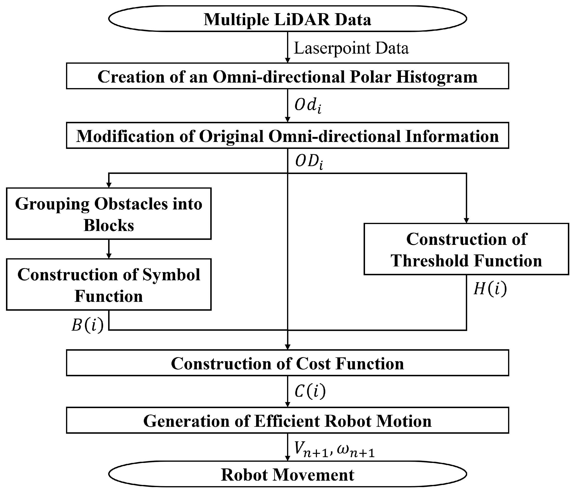
The proposed method consists of seven major steps, as illustrated in Figure 1. First off, a multiple LiDAR information based omni-directional histogram is generated. At this stage, a coordinate system transformation process and methods for overcoming the non-uniformity of information are introduced together. This histogram is then modified based on the size of the robot to represent the robot as a point. Consecutive data in the histogram are grouped to generate a symbol function for detecting concave blocks and a threshold function for safety. These functions are utilized to compute a cost function that determines the velocity vector (control inputs) of the robot, enabling time-efficient and collision-free navigation. A detailed explanation of each step is provided in the subsequent sections.

2.1. Creation of an Omni-Directional Polar Histogram

In the proposed method, information is acquired by two LiDAR sensors mounted on the front and rear of the robot. In this process, if the algorithm is performed using each LiDAR sensor data as it is, an accurate histogram cannot be created because the sensor coordinate systems and the robot coordinate system are different. Therefore, in order to create an accurate omni-directional polar histogram, data obtained from the two LiDAR sensors should be transformed into the robot coordinate system as follows:

$$\left[\begin{array}{c}{x}_{FL,i}\\ y_{FL,i}\end{array}\right]=\left[\begin{array}{c}{d}_{FL,i}\cos {\theta }_{FL,i}\\ d_{FL,i}\sin {\theta }_{FL,i}\end{array}\right],i=1,\dots ,720,$$

(1)

$$\left[\begin{array}{c}{x}_{RL,i}\\ y_{RL,i}\end{array}\right]=\left[\begin{array}{c}{d}_{RL,i}\cos {\theta }_{RL,i}\\ d_{RL,i}\sin {\theta }_{RL,i}\end{array}\right],i=1,\dots ,720,$$

(2)

$$\left[\begin{array}{c}{x}_{R,i}\\ y_{R,i}\\ 1\end{array}\right]=\left[\begin{array}{ccc}\cos {\varphi }_{FL}& -\sin {\varphi }_{FL}& t_{x,FL}\\ \sin {\varphi }_{FL}& \cos {\varphi }_{FL}& t_{y,FL}\\ 0& 0& 1\end{array}\right]\left[\begin{array}{c}{x}_{FL,i}\\ y_{FL,i}\\ 1\end{array}\right],i=1,\dots ,720,$$

(3)

$$\left[\begin{array}{c}{x}_{R,j+720}\\ y_{R,j+720}\\ 1\end{array}\right]=\left[\begin{array}{ccc}\cos {\varphi }_{RL}& -\sin {\varphi }_{RL}& t_{x,RL}\\ \sin {\varphi }_{RL}& \cos {\varphi }_{RL}& t_{y,RL}\\ 0& 0& 1\end{array}\right]\left[\begin{array}{c}{x}_{RL,j}\\ y_{RL,j}\\ 1\end{array}\right],j=1,\dots ,720,$$

(4)

where $FL$ and $RL$ are used as subscripts to refer to the front LiDAR and rear LiDAR, respectively. Since each LiDAR sensor covers 0 to 180${}^{\circ }$ with a 0.25${}^{\circ }$ resolution, the number of each LiDAR data is 720. $d_i$ and ${\theta }_i$ represent the i-th measured distance and angle, respectively. In the transformation matrix, $t_x,t_y$, and $\varphi$ are the relative positions and angle between a LiDAR sensor and the center of the robot, respectively. In both equations, the right-hand terms ($x_{FL,i},y_{FL,i}$) and ($x_{RL,j},y_{RL,j}$) denote the coordinates of the points at the i-th and j-th indices measured by LiDAR sensors, respectively. ($x_{R,i},y_{R,i}$) is the robot centered coordinate for the i-th index.

Based on this, the transformed polar histogram $O{d}_i$ and corresponding angle ${\theta }_i$ are represented as follows:

$$O{d}_i=\sqrt{{x_{R,i}}^2+{y_{R,i}}^2},i=1,2,\dots ,1440,$$

(5)

$${\theta }_i={\tan }^{-1}\frac{y_{R,i}}{x_{R,i}},i=1,2,\dots ,1440.$$

(6)

The aforementioned processes are graphically illustrated in Figure 2.

However, as the LiDAR sensor data are originally represented as a histogram in polar coordinates, this process entails intricate calculations that necessitate the conversion from polar coordinates to Cartesian coordinates, followed by a subsequent conversion back to polar coordinates. In this study, the raw LiDAR sensor data undergo direct conversion into new robot-centered data. First off, the i-th LiDAR data $d_i$ are directly transformed into the j-th new data $OR{d}_j$ as follows:

$$OR{d}_j=d_i^2+t_x^2-2\left|t_x\right|\cos (\pi -{\theta }_i),i=1,2,\dots ,720,$$

(7)

where $t_x$ denotes the translation between the centers of the sensor and the robot. It is assumed that the front and rear sensors are positioned to align with the direction of the robot’s center. Subsequently, the corresponding angle $R{\theta }_j$ can be computed using $OR{d}_j$, $d_i$, and $t_x$ as follows:

$$R{\theta }_j={\cos }^{-1}\left(\frac{t_x^2+OR{d}_j^2-d_i^2}{2|t_x|OR{d}_j}\right),i=1,2,\dots ,720,$$

(8)

The transformed data do not yield a histogram with uniformly spaced intervals in all directions centered on the robot. Based on all computed pairs, a uniformly spaced omni-directional histogram $O{d}_j$ is created as follows:

$$O{d}_j=\min \left(OR{d}_i\right),\mathrm{for}\mathrm{all}i\mathrm{where}{\theta }_j=INT\left(R{\theta }_i\right),$$

(9)

where $INT(·)$ represents a function that returns the integer value of the provided input. Equations (7)–(9) are carried out for each LIDAR sensor, and if there are two sensors, they will be performed twice. When multiple pairs are calculated within the angular resolution, the minimum distance excluding zero is chosen, as shown in Figure 3a. Furthermore, to compute distance values for certain angles that are not sensed, such as the left and right sides of the robot, we suggest an interpolation method using linear regression, as shown in Figure 3b. These processes apply to one LiDAR and are equally applicable to the other LiDAR.

2.2. Modification of Original Omni-Directional Information

In the conventional approach, the original information is altered by considering all angles. However, in omni-directional information, the absence of angular constraints can lead to computational challenges with cosine and sine functions. For example, when $y_{ij}$ exceeds $|{90}^{\circ }|$, the cosine function sets it to a negative value. Moreover, nearby obstacles located in the opposite direction can influence the $O{d^{\prime }}_{ij}$ value due to the symmetry of trigonometric functions. To mitigate these issues, the angle difference $y_{ij}$ is restricted to angles less than ${90}^{\circ }$ as follows:

$$\left|y_{ij}\right|\le {90}^{\circ },$$

(10)

$$s_{ij}=O{d}_j\sin \left|y_{ij}\right|,$$

(11)

$$O{d^{\prime }}_{ij}=\left\{\begin{array}{cc}O{d}_i,\hfill & s_{ij}>R\hfill \\ O{d}_i,\hfill & {(s}_{ij}\le R)\mathrm{and}(O{d}_j\cos \left|y_{ij}\right|>O{d}_i)\hfill \\ O{d}_j\cos \left|y_{ij}\right|,\hfill & \mathrm{others}\hfill \end{array}\right.$$

(12)

$$O{D}_i=\min \left(O{d^{\prime }}_{ij}\right)-R.$$

(13)

The result of $O{D}_i$ is shown in Figure 4.

2.3. Grouping Obstacles into Blocks

In this section, the distance between points obtained from two consecutive indices is computed. If the result is smaller than $d_{thr}$, the two points are involved in a group (block). This allows us to determine the surrounding environment in units of objects instead of points. In the original research, $d_{thr}$ should be larger than R. However, grouping the points solely based on R can lead to incorrect grouping. For instance, it may cause the entire area to be represented as a single block, as shown in Figure 5a. This can cause difficulty in discriminating concave blocks, which will be explained later. In this study, when the number of blocks is one, we apply an additional iteration to reduce $d_{thr}$ by half. In the conventional method, due to its limited range in a semicircle, information from the first and last grouped obstacles may be different. In contrast, the proposed method calculates the polar histogram circularly, which groups obstacles seamlessly. Figure 6 illustrates the results obtained through this process.

2.4. Construction of Cost Function

According to [16], a cost function is defined as follows:

$$C\left(i\right)=\frac{B\left(i\right)H\left(i\right){OD}_i}{k_1{h}_g+k_2{h}_o+k_3},$$

(14)

where in the numerator, $B\left(i\right)$ represents the symbol function and $H\left(i\right)$ represents the threshold function. The symbol function is responsible for setting the indices included in the concave block (obtained in the previous section) to zeros while setting the indices corresponding to the non-concave blocks to ones. Figure 7 displays the results obtained from the symbol function.

To construct the threshold function, the first step is to compute the safety distance $d_{safe}$ [26] as follows:

$$d_{safe}=K(\frac{v}{v_{max}}{R}_{min}+vT),$$

(15)

where K is a coefficient of the safety distance, v is the robot’s velocity, $v_{max}$ is the maximum velocity, $R_{min}$ is the minimum rotation angle at maximum speed, and T is the computational period. The indices of the threshold function are set by comparing $d_{safe}$ and $O{D}_i$. If $O{D}_i$ is included in $d_{safe}$, the indices are set to zero, indicating that an obstacle is located near the robot. On the other hand, if $O{D}_i$ is excluded from $d_{safe}$, the indices are set to one.

In the denominator, $k_1$, $k_2$, and $k_3$ are purpose-oriented nonzero coefficients. $k_1$$h_g$ represents the cost of angular deviation from the target point, and $k_2$$h_o$ represents the cost of deviation between the current direction of the robot and each candidate direction. $k_3$ is a constant that allows the denominator to represent values greater than zero. In Figure 8, $h_r$ is the heading angle of the robot in the global coordinate system, $h_o$ is the angle between the obstacle and the robot, and $h_g$ is the angle between the obstacle and the target point.

$$C\left(m\right)=\max \left(C\right(i\left)\right)i=1,2,\dots ,1440.$$

(16)

The direction with the greatest cost among the 1440 costs calculated through the cost function becomes the target direction in which the robot should move. Figure 9 shows the final result of the proposed method.

2.5. Generation of Efficient Robot Motion

In this section, the backward motion and smoothing factor were considered together to increase the efficiency of the robot motion. The calculation formula is as follows:

$$v_{n+1}=\left\{\begin{array}{cc}sgn\left(\cos \frac{m\pi }{720}\right)v_{max}/\zeta \hfill & ,\mathrm{if}\sqrt{2a{D}_m}>v_{max}\hfill \\ sgn\left(\cos \frac{m\pi }{720}\right)\sqrt{2a{D}_m}/\zeta \hfill & ,\mathrm{others}\hfill \end{array}\right.,$$

(17)

where $v_{max}$ is the maximum speed of the robot, a is the maximum acceleration of the robot, $sgn\left(\cos \frac{m\pi }{720}\right)$ can generate the motion of the robot that can move backward, and $\zeta$ is a smoothing factor of the robot movement. When the robot is moving backward, its angular speed needs to be adjusted according to its movement. Thus, the angular speed ${\omega }_{n+1}$ can be computed as follows:

$${\omega }_{n+1}=\left\{\begin{array}{cc}({\omega }_m+\pi )\eta \hfill & ,\mathrm{if}{\theta }_m<-\frac{\pi }{2}\hfill \\ ({\omega }_m-\pi )\eta \hfill & ,\mathrm{else}\mathrm{if}{\theta }_m>\frac{\pi }{2}\hfill \\ {\omega }_m\eta \hfill & ,\mathrm{others}\hfill \end{array}\right.,$$

(18)

where ${\theta }_m$ is the angle of the maximum cost. $\eta$ is a coefficient for smooth rotation, which is less than one. The velocity of robot is determined using Equations (17) and (18), and its direction can be inverted based on the direction difference at time n and $n+1$. The discrete change in direction in the robot’s velocity can lead to unusual robot movements. To induce continuous robot motion, we proposed smoothing factors for velocity.

3. Experiment

In this section, several performance evaluations and comparisons with the conventional method [16,20] were carried out in terms of the accumulated amount of rotations, total traveling distance, and time. The designed robot equipped with RPLiDAR A3 LiDAR sensors on the front and rear is shown in Figure 10. Its 25 m range radius and 0.25${}^{\circ }$ angular resolution were sufficient to detect objects. Cartographer-based localization and mapping [26] were performed in the background. If a map was already built by the cartographer, a Monte-Carlo localization method was also carried out for more correct positioning [27,28]. Parameters were determined according to Equations (12), (14), (17) and (18). The parameter regarding the robot size, R, was set to 0.6 m. $k_1$, $k_2$, and $k_3$ were defined as 10, 0.2, and 1, respectively. The maximum linear velocity, $v_{max}$, and the linear acceleration, a, were set to 0.3 m/s and 0.25 m/s${}^2$, respectively. The coefficient for smooth rotation, $\eta$, was 2/3. The distance between the start point and the goal point in each experiment was set to 5 m. Experimental scenarios were organized by humans and static obstacles.

3.1. First Experiment in a Crowded Environment

The scenario of the first experiment is illustrated in Figure 11. The red arrows indicate the paths of a crowd, while the red dots indicate their current position. Figure 12 shows the robot trajectories of the two methods over time. Unlike the conventional method with many rotations in avoidance, the proposed method quickly avoids the crowd after moving backward. The evaluation results for the accumulated rotation, total traveling distance, and time are shown in

Table 1. The evaluation results of the first experiment.

Methods	Total Traveling Time (s)	Total Traveling Distance (m)	Accumulated Amount of Rotation (rad)
Conventional method [20]	28.32	8.48	13.63
Proposed method	26.85	7.18	8.02

. As shown in Table 1, when the robot encounters a crowd, the conventional method causes the robot to rotate a lot and takes a long time for avoidance. As a result, the robot had a long traveling distance. However, the proposed method shortens the travel time by significantly reducing the amount of rotations and by quickly avoiding the collision situation after reversing. These advantages can bring greater strength in a practical situation. For instance, by reducing the amount of rotations, unexpected collisions and the performance degradation of localization techniques such as simultaneous localization and mapping (SLAM) can be minimized.

3.2. Second Experiment in an Environment with Humans and Obstacles

The scenario in the second experiment is illustrated in Figure 13. As mentioned previously, the red arrow represents the path of a human, and the red dot indicates their current location. Figure 14 shows the robot trajectories of the two methods over time. When the path between two static obstacles that the robot can pass through is obstructed by a human, the robot utilizing conventional methods takes a wide turn to avoid the obstacle. In contrast, the proposed method promptly navigates backward and efficiently avoids the obstacle.

The evaluation results for the accumulated amount of rotations, total traveling distance, and time are shown in

Table 2. The evaluation results of the second experiment.

Methods	Total Traveling Time (s)	Total Traveling Distance (m)	Accumulated Amount of Rotations (rad)
Conventional method [20]	31.8	9.71	13.8
Proposed method	21.3	5.75	4.49

.

As shown in Table 2, the conventional method greatly increases both the amount of rotations and the traveling distance because the robot rotates significantly to avoid the obstacle and the human, but the proposed method shortens the traveling time by greatly reducing the amount of rotations and the total traveling distance through moving backwards. As mentioned earlier, this advantage becomes particularly valuable in real-world scenarios. By minimizing the amount of rotations, the risk of unexpected collisions and the performance degradation of SLAM can be significantly reduced.

4. Discussion

In this section, the experimental results of the conventional method and the proposed method are additionally analyzed. In particular, in each experiment, the heading, linear velocity, and angular velocity of the robot at key points in time when the conventional method and the proposed method took a different path were confirmed and analyzed.

4.1. Additional Analysis for the First Experiment

When the robot is surrounded by a crowd, the robot heading and control inputs computed by each method are shown in Figure 15 and described in

Table 3. Robot heading and control inputs in collision avoidance in Figure 15a.

Methods	${\mathit{\theta }}_{\mathit{m}}$ (${}^{\circ }$)	${\mathit{v}}_{\mathit{n}+1}$ (m/s)	${\mathit{\omega }}_{\mathit{n}+1}$ (rad/s)
Conventional method [20]	0	0.3	1.0
Proposed method	164.54	−0.3	−0.18

and

Table 4. Robot heading and control inputs in collision avoidance in Figure 15b.

Methods	${\mathit{\theta }}_{\mathit{m}}$ (${}^{\circ }$)	${\mathit{v}}_{\mathit{n}+1}$ (m/s)	${\mathit{\omega }}_{\mathit{n}+1}$ (rad/s)
Conventional method [20]	90	0.3	1.0
Proposed method	125.3	−0.3	0.64

, respectively.

In the conventional approach, $O{d}_i$ values for all i are less than the robot size, R, due to people approaching from the front. As a result, $O{D}_i$ values for all i are zeros and the corresponding costs are also zeros. Since there is no maximum value for the cost function, the direction corresponding to the first index, 90${}^{\circ }$, is chosen as the robot’s next heading, as shown in Figure 15a. Due to the $O{D}_i$, the robot has zero linear velocity. In addition, ${\omega }_{n+1}$ is calculated as 1.0 rad/s $(\eta =\frac{2}{3})$ to turn 90${}^{\circ }$. This can be interpreted as necessitating a high rotational angular velocity to achieve a significant rotation angle. On the other hand, the proposed algorithm constructs a cost function based on an omni-directional polar histogram. The next heading direction is achieved as 164.54${}^{\circ }$, which is the direction with the maximum value of the cost function. Since the robot has a linear speed of −0.3 m/s, it only requires a rotation of 15.46${}^{\circ }$ (180–164.54${}^{\circ }$). Consequently, it rotates a minimal amount at a speed of −0.18 rad/s compared to the conventional method, effectively preventing any additional collisions with nearby people.

As shown in Figure 15b and Table 4, while the conventional method continues to rotate and remains unable to escape, the proposed method rapidly attempts to escape in the direction with the highest cost after moving backward. These observations led to significant improvements in the total experimental results.

4.2. Additional Analysis for the Second Experiment

In the second experiment, when the path between two static obstacles that the robot could pass through is blocked by a human, the heading result and control inputs of each method are shown in Figure 16 and described in

Table 5. Robot heading and control inputs in collision avoidance in Figure 16a.

Methods	${\mathit{\theta }}_{\mathit{m}}$ (${}^{\circ }$)	${\mathit{v}}_{\mathit{n}+1}$ (m/s)	${\mathit{\omega }}_{\mathit{n}+1}$ (rad/s)
Conventional method [20]	86.75	0.3	1.0
Proposed method	173.25	−0.3	−0.07

and

Table 6. Robot heading and control inputs in collision avoidance in Figure 16b.

Methods	${\mathit{\theta }}_{\mathit{m}}$ (${}^{\circ }$)	${\mathit{v}}_{\mathit{n}+1}$ (m/s)	${\mathit{\omega }}_{\mathit{n}+1}$ (rad/s)
Conventional method [20]	90	0.3	1.0
Proposed method	−54.84	0.3	−0.62

, respectively.

In Figure 16a, the robot using the conventional method rotates in the direction of 86.75${}^{\circ }$, which corresponds to the maximum value of the cost function. Despite the absence of obstacles behind the robot, its movement is constrained by the limited range of the polar histogram. However, the proposed method has room to detect situational changes within the sensing range through backward motion. Figure 16b shows the situation where a person passed by and disappeared, while the conventional method continues to drive along the static object, it is forced to move in the opposite direction (90${}^{\circ }$ denoted in Table 6) due to the lack of awareness of the situation change. In contrast, the proposed method promptly recognizes the changed situation (the person blocking the road disappears) and quickly navigates through the passage. As with the previous experiment, these fragmentary results were cumulative and resulted in a significant improvement in the overall experimental results.

5. Conclusions

In this study, an extended vector polar histogram (EVPH) method is proposed for robot navigation that incorporates data from two or more LiDAR sensors to achieve omni-directional sensing. The proposed EVPH method directly transforms the LiDAR sensor coordinate systems into a robot coordinate system to obtain an omni-directional histogram. In addition, it creates a symbol function for detecting concave blocks and a threshold function for safety. These functions are combined to compute a cost function that determines the next robot heading. Finally, based on the heading, the proposed robot’s velocity vector is computed for time-efficient and safe navigation. The proposed EVPH method was evaluated through experiments in environments with humans and obstacles, showing that the robot can navigate safely and efficiently in terms of the accumulated amount of rotations, total traveling distance, and time. In the future, we aim to enhance the robustness of the proposed method in congested environments by integrating dynamic object estimation methods with the adaptation of fixed parameters such as $k_1$ and $k_2$.

References

- Yan, K.; Ma, B. Mapless Navigation Based on 2D LIDAR in Complex Unknown Environments. Sensors 2020, 20, 5802. [Google Scholar] [CrossRef] [PubMed]
- Díaz, D.; Marín, L. VFH+D: An Improvement on the VFH+ Algorithm for Dynamic Obstacle Avoidance and Local Planning. IFAC-PapersOnLine 2020, 53, 9590–9595. [Google Scholar] [CrossRef]
- Gao, F.; Li, C.; Zhang, B. A Dynamic Clustering Algorithm for Lidar Obstacle Detection of Autonomous Driving System. IEEE Sens. J. 2021, 21, 25922–25930. [Google Scholar] [CrossRef]
- Krell, E.; Sheta, A.; Balasubramanian, A.; King, S. Collision-Free Autonomous Robot Navigation in Unknown Environments Utilizing PSO for Path Planning. J. Artif. Intell. Soft Comput. Res. 2019, 9, 267–282. [Google Scholar] [CrossRef] [Green Version]
- Rafai, A.N.A.; Adzhar, N.; Jaini, N.I. A Review on Path Planning and Obstacle Avoidance Algorithms for Autonomous Mobile Robots. J. Robot. 2022, 2022, 2538220. [Google Scholar] [CrossRef]
- Khatib, O. Real-Time Obstacle Avoidance for Manipulators and Mobile Robots. In Proceedings of the 1985 IEEE International Conference on Robotics and Automation, St. Louis, MO, USA, 24–28 March 1985; pp. 500–505. [Google Scholar] [CrossRef]
- Cheng, G.; Zelinsky, A. A physically grounded search in a behavior based robot. In Proceedings of the Eighth Australian Joint Conference on Artificial Intelligence, Wollongong, NSW, Australia, 21–22 November 1995; pp. 547–554. [Google Scholar]
- Dai, J.; Wang, Y.; Wang, C.; Ying, J.; Zhai, J. Research on Hierarchical Potential Field Method on Path Planning for UAV. In Proceedings of the 2018 2nd IEEE Advanced Information Management, Communicates, Electronic and Automation Control Conference (IMCEC), Xi’an, China, 25–27 May 2018; pp. 529–535. [Google Scholar] [CrossRef]
- Borenstein, J.; Koren, Y. Real-Time Obstacle Avoidance for Fast Mobile Robots. IEEE Trans. Syst. Man Cybern. 1989, 19, 1179–1187. [Google Scholar] [CrossRef] [Green Version]
- Borenstein, J.; Koren, Y. The Vector Field Histogram-Fast Obstacle Avoidance for Mobile Robots. IEEE Trans. Robot. Autom. 1991, 7, 278–288. [Google Scholar] [CrossRef] [Green Version]
- Ulrich, I.; Borenstein, J. VFH+: Reliable Obstacle Avoidance for Fast Mobile Robots. In Proceedings of the 1998 IEEE International Conference on Robotics and Automation, Leuven, Belgium, 16–20 May 1998; Volume 2, pp. 1572–1577. [Google Scholar] [CrossRef]
- Ulrich, I.; Borenstein, J. VFH*: Local obstacle avoidance with look-ahead verification. In Proceedings of the IEEE International Conference on Robotics and Automation (ICRA’00), San Francisco, CA, USA, 24–28 April 2000; Volume 3, pp. 2505–2511. [Google Scholar] [CrossRef]
- Guyonneau, R.; Mercier, F.; Oliveira Freitas, G. LiDAR-Only Crop Navigation for Symmetrical Robot. Sensors 2022, 22, 8918. [Google Scholar] [CrossRef] [PubMed]
- Koren, Y.; Borenstein, J. Potential Field Methods and Their Inherent Limitations for Mobile Robot Navigation. In Proceedings of the 1991 IEEE International Conference on Robotics and Automation, Sacramento, CA, USA, 9–11 April 1991; Volume 2, pp. 1398–1404. [Google Scholar] [CrossRef]
- An, D.; Wang, H. VPH: A New Laser Radar Based Obstacle Avoidance Method for Intelligent Mobile Robots. In Proceedings of the Fifth World Congress on Intelligent Control and Automation, Hangzhou, China, 15–19 June 2004; Volume 5, pp. 4681–4685. [Google Scholar] [CrossRef]
- Gong, J.; Duan, Y.; Man, Y.; Xiong, G. VPH+: An Enhanced Vector Polar Histogram Method for Mobile Robot Obstacle Avoidance. In Proceedings of the 2007 International Conference on Mechatronics and Automation, Harbin, China, 5–8 August 2007; pp. 2784–2788. [Google Scholar] [CrossRef]
- Lee, S.; Eoh, G.; Lee, B. Robust Robot Navigation Using Polar Coordinates in Dynamic Environments. J. Ind. Intell. Inf. 2014, 2, 6–10. [Google Scholar] [CrossRef]
- Liu, K.; Gong, J.; Chen, H. VPH+ and MPC Combined Collision Avoidance for Unmanned Ground Vehicle in Unknown Environment. arXiv 2018, arXiv:1805.08089. [Google Scholar]
- Lee, S.; Lee, H.; Lee, B. Visually-Extended Vector Polar Histogram Applied to Robot Route Navigation. Int. J. Control Autom. Syst. 2011, 9, 726–736. [Google Scholar] [CrossRef]
- Wang, H.; Wang, L.; Li, J.; Pan, L. A Vector Polar Histogram Method Based Obstacle Avoidance Planning for AUV. In Proceedings of the 2013 MTS/IEEE OCEANS—Bergen, Bergen, Norway, 10–13 June 2013; pp. 1–5. [Google Scholar] [CrossRef]
- Simmons, R. The Curvature-Velocity Method for Local Obstacle Avoidance. In Proceedings of the IEEE International Conference on Robotics and Automation, Minneapolis, MN, USA, 22–28 April 1996; pp. 3375–3382. [Google Scholar] [CrossRef]
- Brock, O.; Khatib, O. High-Speed Navigation Using the Global Dynamic Window Approach. In Proceedings of the IEEE International Conference on Robotics and Automation, Detroit, MI, USA, 10–15 May 1999; pp. 341–346. [Google Scholar] [CrossRef]
- Fernández, J.L.; Sanz, R.; Benayas, J.; Diéguez, A.R. Improving Collision Avoidance for Mobile Robots in Partially Known Environments: The Beam Curvature Method. Robot. Auton. Syst. 2004, 46, 205–219. [Google Scholar] [CrossRef]
- Shi, C.; Wang, Y.; Yang, J. A Local Obstacle Avoidance Method for Mobile Robots in Partially Known Environment. Robot. Auton. Syst. 2010, 58, 425–434. [Google Scholar] [CrossRef]
- Molinos, E.; Llamazares, Á.; Ocaña, M.; Herranz, F. Dynamic Obstacle Avoidance based on Curvature Arcs. In Proceedings of the IEEE/SICE International Symposium on System Integration, Tokyo, Japan, 13–15 December 2014; pp. 186–191. [Google Scholar] [CrossRef]
- Hess, W.; Kohler, D.; Rapp, H.; Andor, D. Real-time Loop Closure in 2D LIDAR SLAM. In Proceedings of the 2016 IEEE International Conference on Robotics and Automation (ICRA), Stockholm, Sweden, 16–21 May 2016; pp. 1271–1278. [Google Scholar] [CrossRef]
- Ueda, R. Syokai Kakuritsu Robotics (Lecture Note on Probabilistic Robotics); Kodansya: Tokyo, Japan, 2019; ISBN 978-40-6517-006-9. [Google Scholar]
- Ueda, R.; Arai, T.; Sakamoto, K.; Kikuchi, T.; Kamiya, S. Expansion Resetting for Recovery from Fatal Error in Monte Carlo Localization—Comparison with Sensor Resetting Methods. In Proceedings of the 2004 IEEE/RSJ International Conference on Intelligent Robots and Systems (IROS), Sendai, Japan, 28 September–2 October 2004; Volume 3, pp. 2481–2486. [Google Scholar] [CrossRef]
Figure 1.
Flowchart of the proposed method. Multiple LiDAR sensors are used to create a robot-centric omni-directional histogram. During this process, coordinate system transformations are considered. The omni-directional histogram undergoes a modification process to prevent collisions, taking into account the size of the robot. Subsequently, point data are grouped and a threshold function is constructed to enhance stability. The final robot’s moving direction is calculated from the result of the cost function, which generates linear and angular velocities in the direction of stability. Consequently, the robot can move efficiently without colliding at any given moment.
Figure 2.
An example of the construction process for a robot-centered omni-directional polar histogram. Original LiDAR data in (a) are represented in the Cartesian coordinate system as shown in (b). The coordinates are then transformed using the geometric relation between the sensor and the robot as shown in (c). Finally, the transformed coordinates are represented in the polar coordinate system, resulting in a robot-centered omni-directional polar histogram represented in (d). These processes can be streamlined by employing a direct transformation approach proposed in this study.
Figure 3.
Constructed omni−directional polar histogram based on the direct transformation. In (a), and are compared in the polar coordinate system. In (b), shows its strength based on linear interpolation and uniform representation.
Figure 4.
Modification of the omni−directional polar histogram. In (a,b), and are compared.
Figure 5.
An example problem involving grouping obstacles according to . In (a), the result is for = 1.2, which is a large value, causing the entire area to be represented as a single block. In (b), the result is for = 0.1. By examining the size of the cluster represented by the red straight line, it can be observed that the entire area is appropriately clustered.
Figure 6.
The result of grouped blocks. The proposed method checks the polar histogram circularly while grouping obstacles seamlessly.
Figure 7.
Visualization of the symbol function. The function has zeros in concave blocks (red). In non-concave blocks, ones are assigned (black). As a binary function, it plays a crucial role in influencing the cost function, prompting the robot to move towards non-concave blocks.
Figure 8.
The geometric meaning of , , and . represents the robot’s heading angle in the global coordinate system, denotes the angle between the obstacle and the robot, and represents the angle between the obstacle and the target point. To influence the cost function, and are multiplied by and , respectively.
Figure 9.
Visualization of the cost function and target direction. The target direction (indicated in red) is properly determined as a result of the cost function.
Figure 10.
Illustration of the designed robot and equipped sensors. The robot is equipped with two RPLiDAR A3 modeled sensors as shown in (a). In (b), the red semicircle indicates the area scanned by the front LiDAR sensor, while the blue semicircle indicates the area scanned by the rear LiDAR sensor.
Figure 11.
The first scenario. The red arrows indicate the paths of a crowd. The solid red circles and dotted red circles represent their current positions, and previous positions, respectively.
Figure 12.
The trajectory comparison of two methods in the first experiment. The blue line represents the result of the conventional method, while the orange line shows the result of the proposed method. The red arrows indicate the paths of a crowd. The solid red circles and dotted red circles represent their current positions, and previous positions, respectively. Unlike the conventional method that involves multiple rotations during avoidance, the proposed method rapidly maneuvers to avoid obstacles by moving backward. (a) t = 6, (b) t = 10, (c) t = 30.
Figure 13.
The scenario of the second experiment. The blue blocks represent static obstacles. The red arrow indicates the path of the human. The solid red circle and dotted red circle represent the current position, and the previous position of human, respectively.
Figure 14.
The trajectory comparison of the two methods in the second experiment. The blue line represents the conventional method, while the orange line represents the proposed method. The red arrow indicates the path of the human. The solid red circle and dotted red circle represent the current position, and the previous position of human, respectively. When the path between two static obstacles, which the robot can typically pass through, is obstructed by a human, conventional methods result in the robot taking a wide turn to avoid the obstacle. However, the proposed method offers a more efficient solution by quickly navigating backward to effectively avoid the obstruction. (a) t = 6, (b) t = 19, (c) t = 30.
Figure 15.
The target direction comparison of the two methods in the first experiment. The blue arrow represents the conventional method, while the orange arrow represents the proposed method. The red arrows indicate the paths of a crowd. The solid red circles and dotted red circles represent their current positions, and previous positions, respectively. The distinct decisions and motions of the two methods at the above time points result in noteworthy differences in the overall outcomes. (a) t = 6, (b) t = 10.
Figure 16.
The target direction comparison of the two methods in the second experiment. The blue arrow represents the conventional method, while the orange arrow represents the proposed method. The red arrow indicates the path of the human. The solid red circle and dotted red circle represent the current position, and the previous position of human, respectively. The distinct decisions and motions of the two methods at the above time points result in noteworthy differences in the overall outcomes. (a) t = 6, (b) t = 9.