

Dynamics of a Circular Foil and Two Pairs of Point Vortices: New Relative Equilibria and a Generalization of Helmholtz Leapfrogging

1
Ural Mathematical Center, Udmurt State University, ul. Universitetskaya 1, 426034 Izhevsk, Russia
2
Laboratory of Mobile Systems, Kalashnikov Izhevsk State Technical University, ul. Studencheskaya 7, 426069 Izhevsk, Russia
*
Author to whom correspondence should be addressed.
Symmetry 2023, 15(3), 698; https://doi.org/10.3390/sym15030698
Submission received: 31 January 2023
/
Revised: 27 February 2023
/
Accepted: 3 March 2023
/
Published: 10 March 2023
(This article belongs to the Special Issue Geophysical Fluid Dynamics and Symmetry)
Abstract
:In this paper, we study the plane-parallel motion of a circular foil interacting with two vortex pairs in an infinite volume of an ideal fluid. We assumed that the circulation of the velocity of the fluid around the foil was zero. We showed that the equations of motion possess an invariant submanifold such that the foil performed translational motion and the vortices were symmetric relative to the foil’s direction of motion. A qualitative analysis of the motion on this invariant submanifold was made. New relative equilibria were found, a bifurcation diagram was constructed, and a stability analysis is given. In addition, trajectories generalizing Helmholtz leapfrogging were found where the vortices passed alternately through each other, while remaining at a finite distance from the foil.
Keywords:
point vortices; ideal fluid; bifurcation diagram; stability; relative equilibria; Poincaré map; Helmholtz leapfroggingMSC:
76M23; 34A051. Introduction
In this paper we investigate the problem of the motion of a circular foil interacting with two pairs of point vortices using the model of an ideal incompressible fluid. A detailed account of the historical development and various versions of this problem is provided in [1,2,3]. Here, we only mention the previously obtained results closely related to the system under consideration.
The equations of motion of two pairs of vortices in an infinite fluid (i.e., in the absence of a foil) demonstrate chaotic scattering [4]. However, these equations possess an invariant manifold where the solution can be obtained explicitly (see, e.g., [5]). This solution corresponds to mirror-symmetric vortex configurations. They include trajectories describing Helmholtz leapfrogging, where the vortices pass alternately through each other while remaining at a finite distance from each other. A detailed stability analysis of the leapfrogging of vortices is given in [6,7].
In [8], the above-mentioned invariant manifold is generalized to the system of vortices with a circular foil, and relative equilibria corresponding to a collinear configuration of vortices and a foil were found. In addition, for vortex pairs with equal strengths, a relative equilibrium was found where the vortices formed a square, and its geometric center was at the center of the foil. By relative equilibria we mean the translational motion of vortices and a foil such that the distances between them remain constant.
The search for the above-mentioned relative equilibria is closely related to equilibrium points of another system describing the motion of vortex pairs around a fixed circular cylinder in an incoming flow. Analogs of relative equilibria from [8], for two vortex pairs in an incoming flow, are presented in [9]. Other equilibrium points, such that both pairs of vortices lie behind the foil, were found by numerical calculations in [10,11]. They are a generalization of the classical Föppl equilibria [12].
In this work, using the reduced equations derived in [1] for the motion of n point vortices and a circular foil, we obtained equations for a foil and two vortex pairs on an invariant manifold corresponding to mirror-symmetric configurations. For these equations, we found fixed points corresponding to relative equilibria. Among them were relative equilibria with vortices behind the foil. They are an analog of the equilibria found in [10,11] for an incoming flow. Next, using the methods of topological analysis of dynamical systems (described, for example, in [13]), we investigated the stability of the found fixed points. The efficiency of the application of the methods of topological analysis to problems of vortex dynamics has been previously shown [13,14,15]. To numerically study the trajectories on an invariant manifold, we constructed a Poincaré map. Using this map, we found trajectories generalizing Helmholtz leapfrogging that is described above.
2. Equations of Motion
Main assumptions. Consider the plane-parallel motion of a cylindrical body (cylinder) in an infinite volume of an ideal fluid with two vortex pairs. Each vortex pair consists of two point vortices with strengths equal in magnitude and opposite in sign. Let the following conditions be satisfied:
- The foil of the body is a circle of radius a with its center of mass at the geometric center of the circle C;
- The circulation of the velocity of the fluid around the foil is zero.
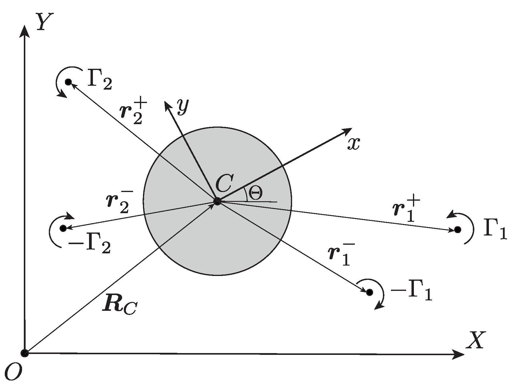
Choose two coordinate systems on a plane perpendicular to the motion of the vortices and the cylinder (see Figure 1):
- A fixed (inertial) coordinate system ;
- A moving coordinate system attached to the foil, with its origin at the center of the circle.
Let be the radius vector of the geometric center of the foil C in the fixed coordinate system . Let us specify the foil’s orientation by the angle between the axes and . Denote the coordinates of the ith pair of vortices in the moving axes by and , where and are the coordinates of the vortices with positive and negative strengths, respectively.
Reduced system. The equations of motion do not explicitly depend on the choice of the origin and the direction of the axes of the fixed coordinate system , so that the vector field of the system possesses symmetry fields. An explicit form of these symmetry fields is presented in the paper [1], which also gives a detailed description of the reduction procedure for the problem of the motion of n point vortices and a circular foil in an ideal fluid.
Choose as variables of the reduced system the coordinates of vortices, the total momentum , and the total angular momentum of the foil and the vortices in the frame . Then, the reduced system has the following form (see [1] for details):
where , is the density of the fluid, and is a Hamiltonian that is given by the relation
where the function has been introduced and m and I are the effective mass and the moment of inertia of the foil, respectively.
Equation (1) is a Hamiltonian system with the following Poisson brackets (only nonzero Poisson brackets are presented):
This Poisson structure is degenerate (its rank is six) and hence possesses the Casimir function
which is also a first integral of the system in (1). Moreover, the reduced system in (1) possesses an additional first integral [1]
Reconstruction of dynamics. In order to define the motion of the foil in the fixed coordinate system from the known solution of the reduced system in (1), it is necessary to use the Noether integrals [1]:
By rotating the fixed axes (i.e., by choosing origin ), we can ensure that the vector composed of the first integrals is directed along the axis , i.e.,
Accordingly, the angle and the variable Y are expressed from (5) as follows:
The evolution of the variable X describing the motion of the foil along the vector of the total momentum is governed by equation [1]:
Discrete symmetries and invariant submanifold. In the analysis of the dynamics of the system in (1), an important role is played not only by the above-mentioned conservation laws (the first integrals and the Poisson tensor), but also discrete symmetries. Let us consider them in more detail.
The reduced system in (1) admits two involutions (time-reversal symmetries). One of them involves rearranging the position of the vortices in the pair and changing the sign of the linear and angular momenta:
and the other has the form
Remark 1.
It is fairly simple to verify the presence of the involutions of and . Indeed, after an appropriate change in variables of the reduced system (without time reversal) the Hamiltonian remains invariant, while the right-hand sides of Equation (1) change their sign. Therefore, in order that the equations remain invariant, it is necessary to reverse the direction of time.
Composing these two involutions, we obtain the following transformation of symmetry for the reduced system:
As is well known, the fixed points of this symmetry form the invariant submanifold of the system in (1):
Throughout the rest of the paper we restrict ourselves to the analysis of the dynamics of a foil and vortices on the invariant submanifold .
Restriction of the system to the invariant submanifold. Let us parameterize manifold using the dimensionless variables and f as follows:
and define the parameters
Thus, for the vortex pair we keep track, in fact, only of the coordinates of the vortex with positive strength, since, knowing them from (7), we can always restore the position of a vortex with negative strength.
Rescaling time as
we obtain equations of motion on the invariant manifold in the following Hamiltonian form:
where the Hamiltonian H is
where , . We note that f in (8) is a parameter that corresponds to the fixed value of the Casimir function (4) of the initial system.
In the system in (8), one should exclude such values of the coordinates where the following hold:
- One of the vortices lies inside the foil
- Vortices in one of the pairs collide
- Vortices from different pairs collide
As can be seen, the Hamiltonian H has a singularity at , , W and on the boundary of and .
We note that Equation (8) is symmetric under the transformation
Therefore, without loss of generality, it can be assumed that, for example, because the trajectories with can be obtained by making the change in variables (10).
The evolution of the variable X is described by the equation
3. Relative Equilibria and Their Stability
We recall the main principles of the stability analysis of fixed points of Hamiltonian systems with two degrees of freedom that we use in what follows (for details, see, e.g., [13]).
Let be a fixed point of the system in (8), which is also a critical point of the Hamiltonian H. Define the following matrices:
- is the linearization matrix of the vector field in a neighborhood of the fixed point;
- is the matrix of the quadratic part of the Hamiltonian (Hessian).
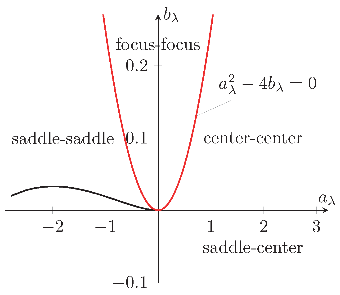
For the system in (1), these are matrices. Each of them is related to an invariant that has a key role in investigating the stability.
- (1)
- The index of the symmetric matrix (i.e., the number of its negative eigenvalues) is denoted by in what follows. It can take the values .
- (2)
- The type of the fixed point defined by the eigenvalues , of the matrix is as follows:
- –
- Center–center (, );
- –
- Saddle–center (, );
- –
- Saddle–saddle (, );
- –
- Focus–focus (),
where and are real numbers. Only a fixed point that is of center–center type is Lyapunov stable.
The index is related to the type of the critical point as follows:
- (1)
- If , then the fixed point is stable and of center–center type;
- (2)
- If , then the fixed point is unstable and of saddle–center type;
- (3)
- If , then the fixed point is of one of three types: center–center, saddle–saddle, or focus–focus. For it to be unstable, it suffices that the matrix has eigenvalues with a nonzero real part. To prove the stability of such a point, it is necessary to use the KAM theorem and it requires that all eigenvalues of the matrix are imaginary numbers and additional nonlinear conditions hold [16].
Thus, to examine the stability of the fixed points, it is in many cases sufficient to calculate its index, and only if is it necessary to specify the type of the point by analyzing the eigenvalues.
When these principles are applied in a standard way, a difficulty arises due to the fact that an analytic formulation of the stability criteria leads to a cumbersome set of inequalities, so that it is often difficult to determine whether there exists a solution satisfying the required criteria. For this reason, on the plane of values of the first integrals
where h is the fixed value of the Hamiltonian , we introduce the extended bifurcation diagram, which is constructed with the following three principles:
- 1.
- We plot the values of corresponding to critical points of ; they form bifurcation curves, and when such a curve is crossed, the topological type of the isoenergetic manifolds changes [13].
- 2.
- We put the index of the corresponding critical point on the bifurcation curves, in [13] it was shown that the index does not change along a smooth branch of the bifurcation curve.
- 3.
- For each branch of the bifurcation curves with the index , we first plot the curves and on the plane of coefficients of the characteristic polynomialand, thus, define possible types of fixed points on the branch and mark the corresponding parts of the branch according to the type of the fixed point.
Thus, the bifurcation diagram described above allows us to answer the questions concerning the existence and stability of the fixed points of Equation (8) (they correspond to relative equilibria of the initial system (1)).
Relative equilibria. We note that the fixed points of the reduced systems in (8) and (9) are given by solutions of four polynomial equations of sufficiently high order. This makes an explicit solution impossible, so we solve this system numerically.
We first consider collinear configurations. For them, the center of the foil and the vortices lie on the axis : and the coordinates and take (constant) values, which satisfy the equations
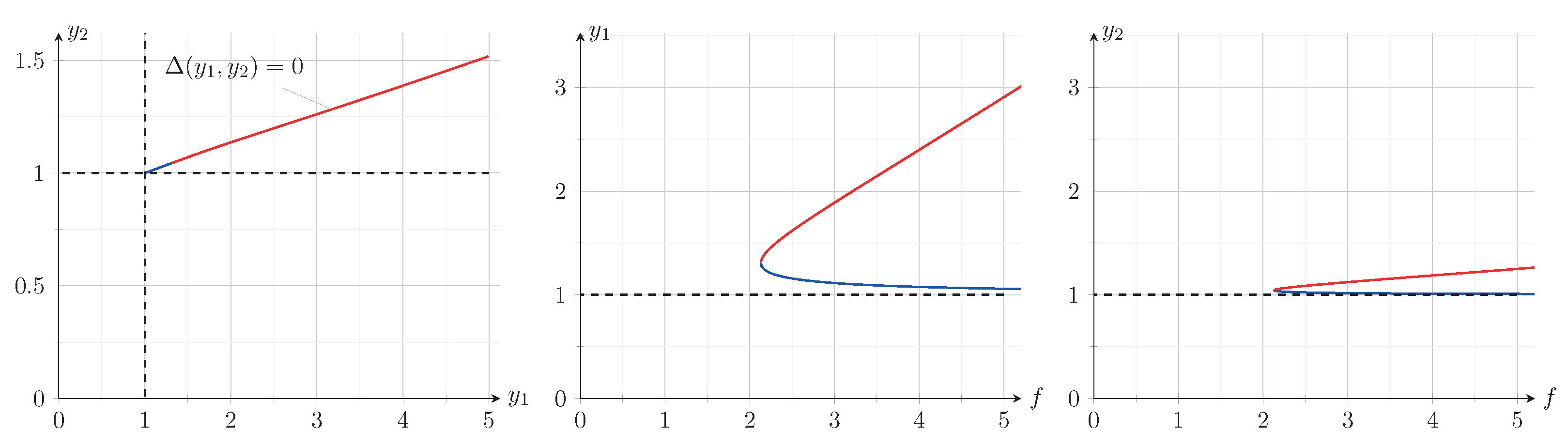
Previously, collinear configurations were found in [8]. It was shown that these two equations have solutions. To describe them, at the first step, we eliminate f from the system in (11) and obtain a solution in the form of a curve on the plane :
If , then the preceding relation defines the curve, which lies in the region , . A typical form of this curve is shown in Figure 2. Then, to define the dependence , it suffices to express f from any equation of (11) and to substitute the values of and satisfying (12). As a result, for the collinear configurations, we obtain the following bifurcation curve:
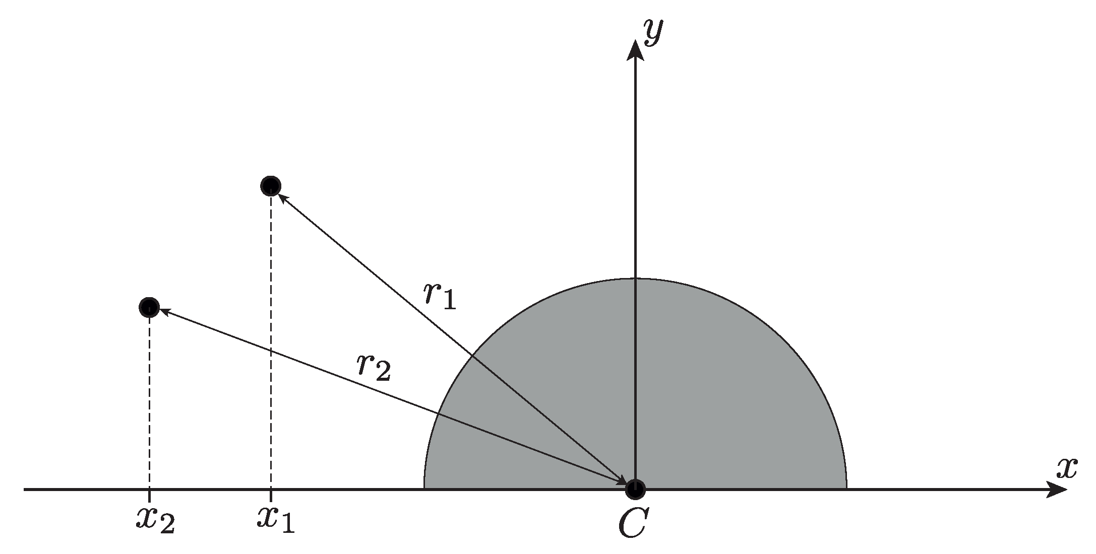
For the foil and one pair of vortices, a relative equilibrium with the vortices behind the foil is known [8,17,18]. Consider the question of the existence of similar solutions for the system with two pairs (see Figure 3). If they exist, then they are fixed points of the system in (8). Without loss of generality, we assume here
To find those equilibria, we fix the values of , , and f and numerically solve the corresponding polynomial system for , using Newton’s algorithm. Then, for the found solutions, using the method of continuation in a parameter, we restore the corresponding bifurcation curves on the plane . Earlier, this method was used to find new configurations of three vortices in a circle [13].
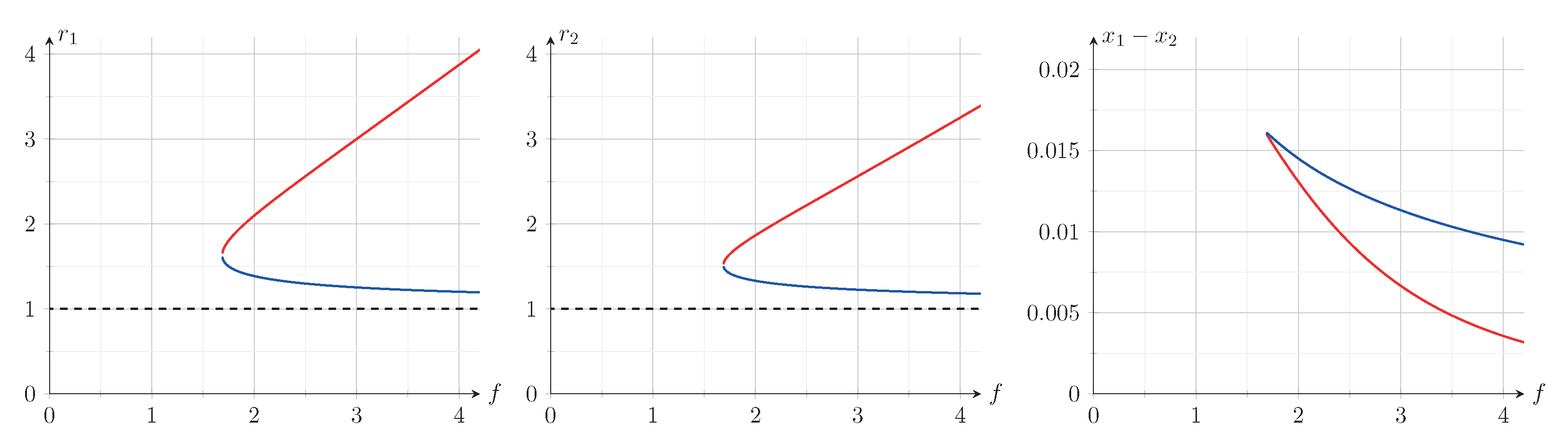
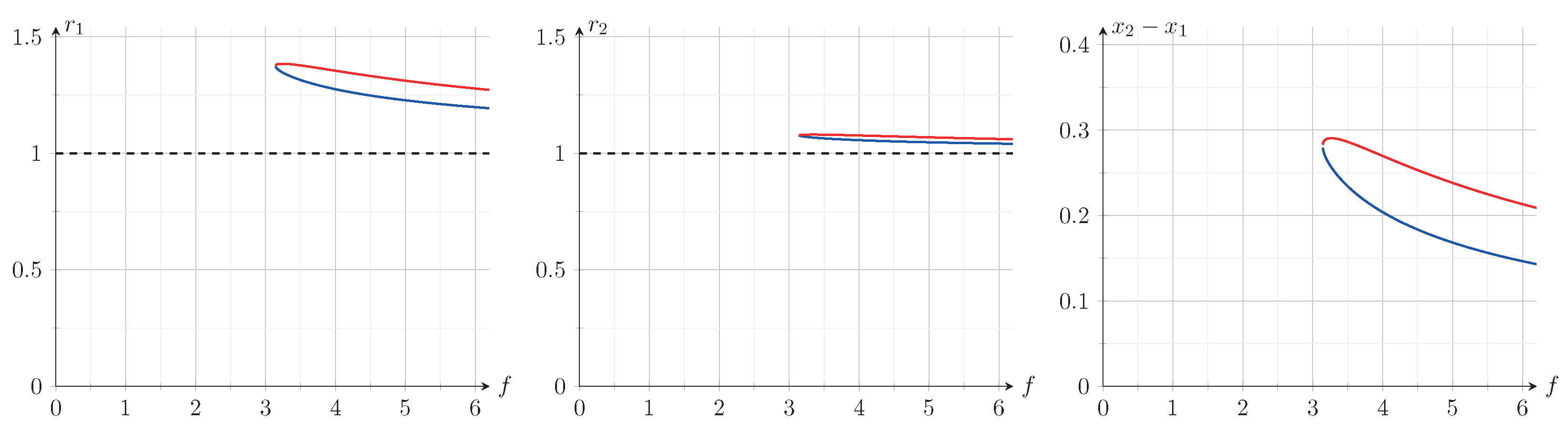
Using the method described above, two more bifurcation curves, and , are found corresponding to the relative equilibria. An example with explicit numerical values of for the found relative equilibria is given in Table 1, the graphs characterizing the arrangement of vortices are shown in Figure 4 and Figure 5, and a bifurcation diagram is shown in Figure 6. From these graphs, several conclusions may be drawn.
- On each bifurcation curve , , a critical point of the cusp type is visible. The values of f and h for each of these cusps correspond to the birth of two isolated relative equilibria. Then, as f increases, each of these relative equilibria persists and forms a branch (smooth part) of a bifurcation curve with the same index. Only the curve has a branch with and, thus, corresponds to stable relative equilibria. Both branches of the bifurcation curves with correspond to fixed points of the saddle–saddle type (see, e.g., Figure 7).
- The branches of the curves and with and , respectively, correspond to relative equilibria where vortices become more distant from the foil as f increases. By contrast, for the other relative equilibria, the distance between vortices and the foil decreases as f increases.
Remark 2.
We do not have a rigorous proof that, for the chosen parameters and , the system in (8) does not possess any other equilibrium points than those mentioned above. However, the resulting bifurcation diagram (Figure 6) is self-consistent (i.e., the change in the type of fixed points occurred at the critical points of the bifurcation curves). We emphasize the importance of the criterion of the breaking of the isolation of a bifurcation curve at degenerate critical points. For example, for a fixed value of f, only one point of each family and was at first found numerically. We then plotted corresponding bifurcation curves in the plane and found that such a bifurcation diagram was not self-consistent. This suggests the existence of additional equilibrium points, which were found later.
In [8], such relative equilibria for equal strengths of vortex pairs (i.e., ) were found where vortices formed a square with a foil at its geometric center. It would be interesting to examine the problem of the existence of such types of equilibria with .
4. Bounded Trajectories: Generalization of the Helmholtz Leapfrogging
In this section, we consider the bounded trajectories of the system in (8), which are not fixed points. For their numerical analysis and visualization we made use of a Poincaré map. We describe its construction in more detail below.
Let us introduce polar coordinates for the positions of the vortices:
According to Section 2, the range of variation of these coordinates is given as , , , and .
Choose a submanifold given by the relation
as a cross-section of the vector field. Next, numerically integrate the system with initial conditions satisfying (13) and use the Hénon method by finding intersections of the trajectory with the chosen cross-section. We finally obtain a Poincaré map of the system (7).
We note that the intersection of the (noncritical) level surface of the Hamiltonian with the cross-section (13) is defined in three-dimensional space
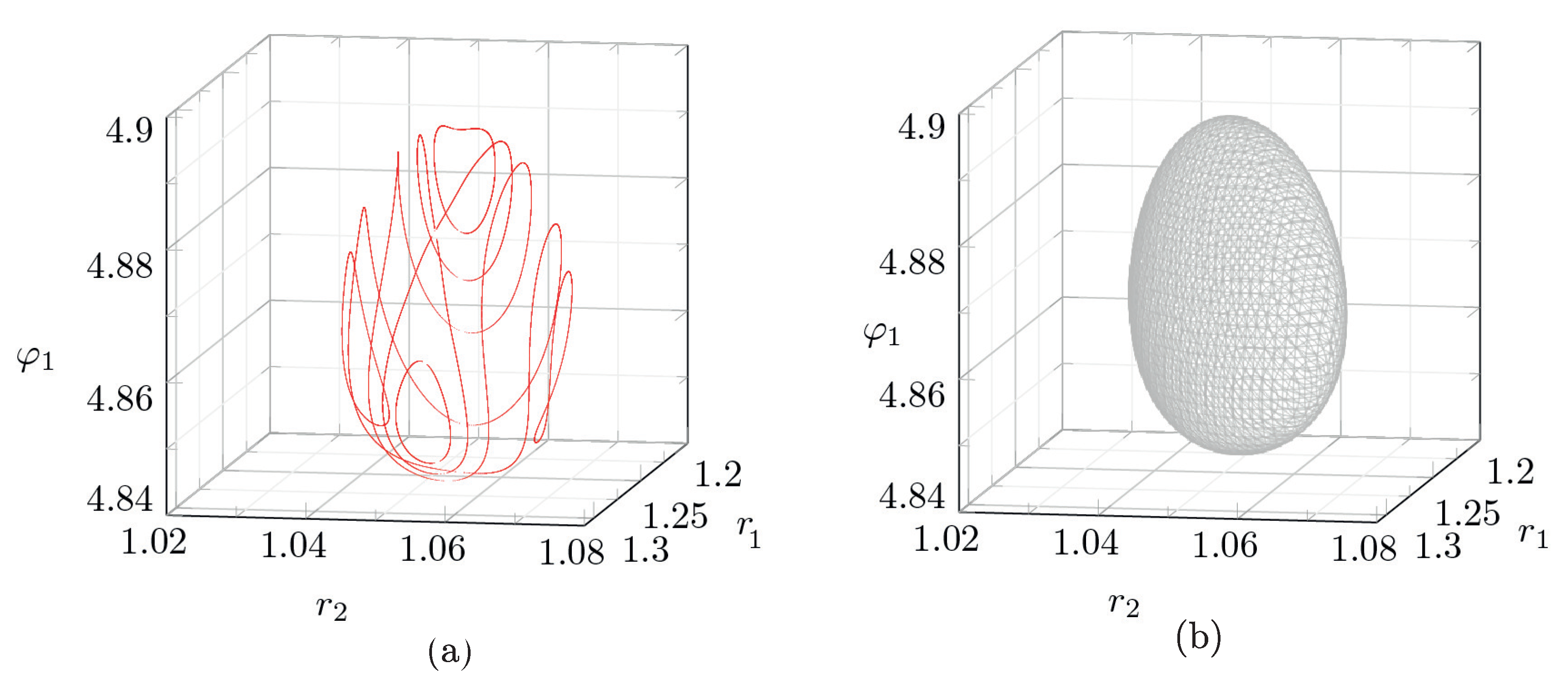
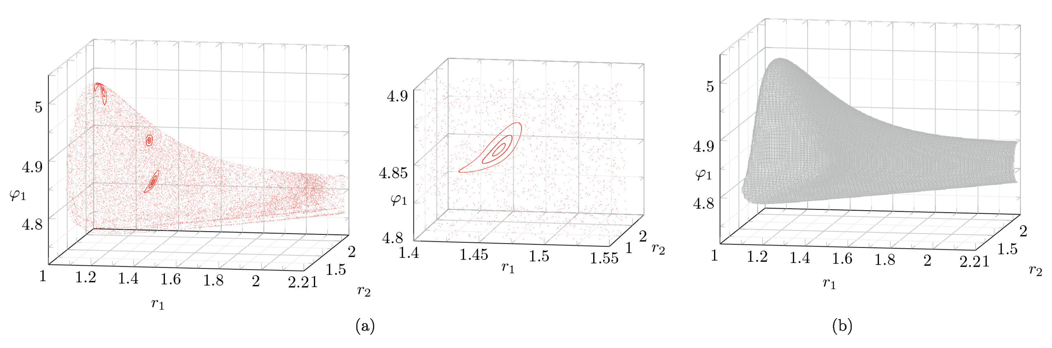
with a two-dimensional manifold , which is disconnected in the general case. Components of have a fairly complex form (see Figure 8b and Figure 9b), and so it is more convenient to plot a map on directly in three-dimensional space than to project it onto some plane.
In addition, the fixed level set of the energy integral can define an unbounded surface that contains scattering trajectories, i.e., trajectories for which one (or several) of the distances , , increase without bounds as . The scattering trajectories may have only a finite number of intersections with the chosen cross-section (13) as . This complicates the use of a Poincaré map for studying the system. Therefore, we first consider the case where the level set of the energy integral has a compact connected component.
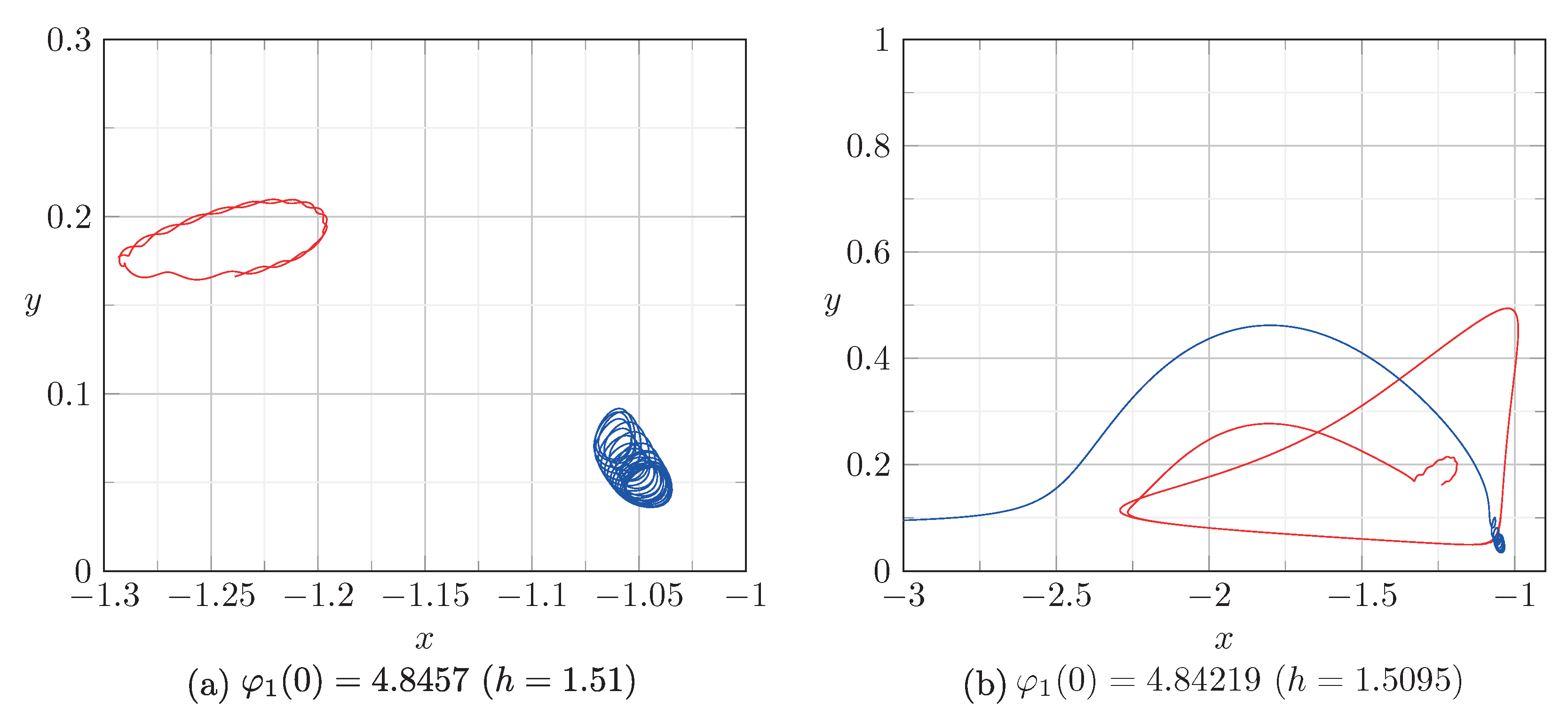
In the preceding section, we pointed out a critical point of the Hamiltonian with index . Hence, in a neighborhood of this point there are compact connected components of and of . An example of such a compact component of and the corresponding Poincaré map is shown in Figure 8, and an example of the trajectory of vortices in the coordinate system is shown in Figure 10a. All trajectories of the system (7) lying on the compact components of correspond to those motions of vortices where they lie in a bounded region near their positions that correspond to critical points with . Further, as h decreases and the branch of the bifurcation curve with is reached, scattering trajectories arise, i.e., the level surface of the Hamiltonian becomes unbounded. An example of such a scattering trajectory is shown in Figure 10b.
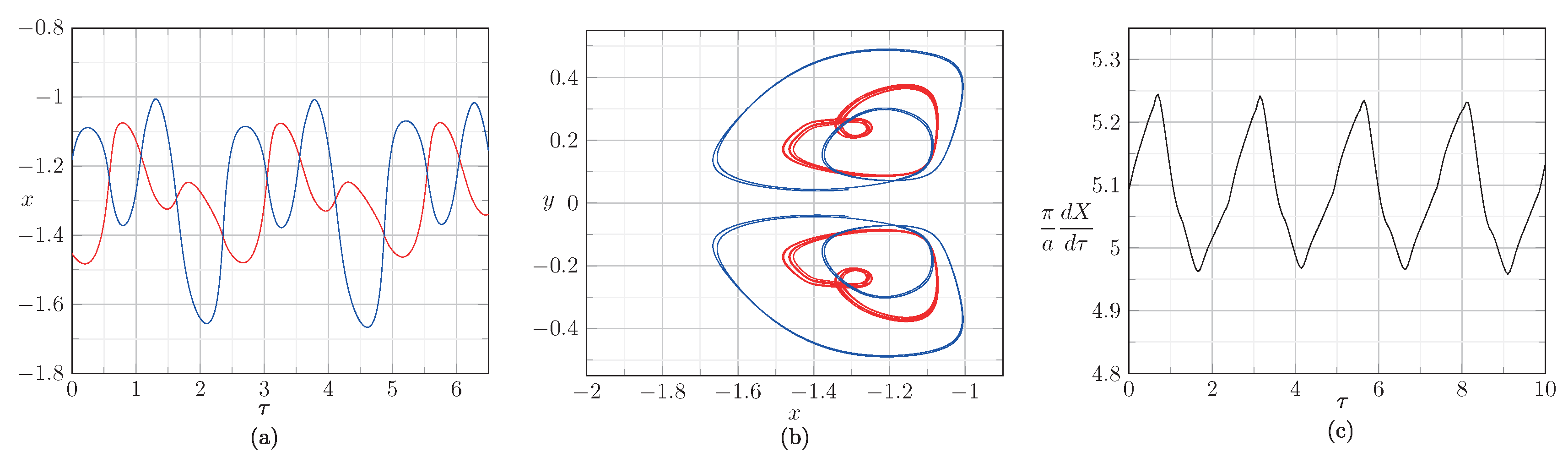
On the noncompact level surface of the Hamiltonian there may also lie bounded trajectories. Figure 9 shows an example of a Poincaré map where has an unbounded connected component. As can be seen, on this map there is a fixed point of period 3, which corresponds to a periodic solution of the system in (7). In addition, in a neighborhood of this point, the map has invariant curves corresponding to quasi-periodic trajectories of the system in (8).
In Figure 11b, the trajectories of vortices in the coordinate system are shown. They correspond to one of the invariant curves on the map of Figure 9a (for details, see (accessed on 1 March 2023) https://www.youtube.com/watch?v=jdW4yOVK_Ww). In this case, the vortex pairs pass alternately through each other, while all distances , , remain bounded (for details, see (accessed on 1 March 2023) https://www.youtube.com/watch?v=PufmBTVEstA). These trajectories generalize Helmholtz leapfrogging of two vortex pairs [6,7].
We note that there are still many open problems in describing the behavior of scattering trajectories in vortex dynamics and the considered system in particular. For example, they include constructing a scattering map and describing trajectories with different types of scattering depending on parameter values and initial conditions (i.e., depending on which of the distances , , increase without a bound). It would also be of interest to search for nonlocal bifurcations of the level surface of the Hamiltonian and to analyze their contribution to the dynamics of the system.
5. Conclusions
Our analysis has allowed us to find two families of relative equilibria where the vortices and the foil move along a straight line with constant velocity, while the vortices are behind the foil. Using the topological methods of stability analysis, we have shown that among them there are equilibria that are stable relative to symmetric perturbations (i.e., perturbations lying on the invariant manifold under consideration). The problem of the stability of these equilibria relative to nonsymmetric perturbations remains unsolved. For numerical analysis of the system’s trajectories we have constructed a Poincaré map. Using this Poincaré map, we have shown the existence of unbounded and bounded trajectories. The bounded trajectories of the system generalize the well-known Helmholtz leapfrogging, and the vortices always remain in a neighborhood of the cylinder. It would be interesting to investigate the problem of stability and conditions for existence of these trajectories depending on the system’s parameters.
Author Contributions
Conceptualization, I.S.M.; Methodology, I.S.M.; Software, I.A.B.; Writing—original draft, I.A.B.; Visualization, I.A.B.; Supervision, I.S.M. All authors have read and agreed to the published version of the manuscript.
Funding
The work of I.A.B. was performed at the Ural Mathematical Center (Agreement no. 075-02-2023-933). The work of I.S.M. was carried out within the framework of the state assignment of the Ministry of Education and Science of Russia (FZZN-2020-0011).
Data Availability Statement
All numerical experiments are described in this paper and can be reproduced without additional information.
Conflicts of Interest
The authors declare no conflict of interest.
References
- Mamaev, I.S.; Bizyaev, I.A. Dynamics of an Unbalanced Circular Foil and Point Vortices in an Ideal Fluid. Phys. Fluids 2021, 33, 087119. [Google Scholar] [CrossRef]
- Ramodanov, S.M.; Sokolov, S.V. Dynamics of a Circular Cylinder and Two Point Vortices in a Perfect Fluid. Regul. Chaotic Dyn. 2021, 26, 675–691. [Google Scholar] [CrossRef]
- Shashikanth, B.N. Dynamically Coupled Rigid Body-Fluid Flow Systems; Springer: Cham, Switzerland, 2021. [Google Scholar]
- Eckhardt, B.; Aref, H. Integrable and Chaotic Motions of Four Vortices: II. Collision Dynamics of Vortex Pairs. Philos. Trans. R. Soc. A 1988, 326, 655–696. [Google Scholar]
- Meleshko, V.V.; Konstantinov, M.Y. Dynamics of Vortex Structures; Naukova Dumka: Kiev, Ukraine, 1993. (In Russian) [Google Scholar]
- Acheson, D.J. Instability of Vortex Leapfrogging. Eur. J. Phys. 2000, 21, 269–273. [Google Scholar] [CrossRef]
- Behring, B.M.; Goodman, R.H. Stability of Leapfrogging Vortex Pairs: A Semi-Analytic Approach. Phys. Rev. Fluid 2019, 4, 124703. [Google Scholar] [CrossRef] [Green Version]
- Shashikanth, B.N. Symmetric Pairs of Point Vortices Interacting with a Neutrally Buoyant Two-Dimensional Circular Cylinder. Phys. Fluids 2006, 18, 127103. [Google Scholar] [CrossRef]
- Moura, M.N.; Vasconcelos, G.L. Four-Vortex Motion around a Circular Cylinder. Phys. Fluids 2013, 25, 073601. [Google Scholar] [CrossRef] [Green Version]
- Seath, D.D. Equilibrium Vortex Positions. J. Spacecr. Rocket. 1971, 8, 72–75. [Google Scholar] [CrossRef]
- Weihs, D.; Boasson, M. Multiple Equilibrium Vortex Positions in Symmetric Shedding from Slender Bodies. AIAA J. 1979, 17, 213–214. [Google Scholar] [CrossRef]
- Föppl, L. Vortex Motion behind a Circular Cylinder; NASA TM 77015; NASA: Washington, DC, USA, 1983.
- Bolsinov, A.V.; Borisov, A.V.; Mamaev, I.S. The Bifurcation Analysis and the Conley Index in Mechanics. Regul. Chaotic Dyn. 2012, 17, 457–478. [Google Scholar] [CrossRef]
- Artemova, E.M.; Vetchanin, E.V. The Motion of an Unbalanced Circular Disk in the Field of a Point Source. Regul. Chaotic Dyn. 2022, 27, 24–42. [Google Scholar] [CrossRef]
- Bizyaev, I.A.; Mamaev, I.S. Qualitative Analysis of the Dynamics of a Balanced Circular Foil and a Vortex. Regul. Chaotic Dyn. 2021, 26, 658–674. [Google Scholar] [CrossRef]
- Arnold, V.I.; Kozlov, V.V.; Neishtadt, A.I. Mathematical Aspects of Classical and Celestial Mechanics, 3rd ed.; Springer: Berlin, Germany, 2006. [Google Scholar]
- Bizyaev, I.A.; Mamaev, I.S. Dynamics of a Pair of Point Vortices and a Foil with Parametric Excitation in an Ideal Fluid. Vestn. Udmurt. Univ. Mat. Mekhanika Kompyuternye Nauk. 2020, 30, 618–627. (In Russian) [Google Scholar] [CrossRef]
- Vasconcelos, G.L.; Moura, M.N.; Schakel, A.M.J. Vortex Motion around a Circular Cylinder. Phys. Fluids 2011, 23, 123601. [Google Scholar] [CrossRef] [Green Version]
Figure 1.
Coordinates and parameters describing a cylindrical foil and two pairs of point vortices in an ideal fluid.
Figure 1.
Coordinates and parameters describing a cylindrical foil and two pairs of point vortices in an ideal fluid.

Figure 2.
A typical curve and dependences and for collinear configurations with , . The red and blue lines denote parts of the curve with the indices and , respectively.
Figure 2.
A typical curve and dependences and for collinear configurations with , . The red and blue lines denote parts of the curve with the indices and , respectively.

Figure 3.
Layout of a foil and point vortices.

Figure 4.
Typical dependences , and for relative equilibria corresponding to the bifurcation curve with , . The red and blue lines denote parts of the curve with the indices and , respectively.
Figure 4.
Typical dependences , and for relative equilibria corresponding to the bifurcation curve with , . The red and blue lines denote parts of the curve with the indices and , respectively.

Figure 5.
Typical dependences , and for the relative equilibria corresponding to the bifurcation curve with , . The red and blue lines denote parts of the curve with the indices and , respectively.
Figure 5.
Typical dependences , and for the relative equilibria corresponding to the bifurcation curve with , . The red and blue lines denote parts of the curve with the indices and , respectively.

Figure 6.
Bifurcation diagram (a) and the dependence , which is the difference between the values of h on the upper and lower branches of the bifurcation curve (b).
Figure 6.
Bifurcation diagram (a) and the dependence , which is the difference between the values of h on the upper and lower branches of the bifurcation curve (b).

Figure 7.
Dependence of the coefficients of the characteristic polynomial for a portion of the bifurcation curve (black) with the index .
Figure 7.
Dependence of the coefficients of the characteristic polynomial for a portion of the bifurcation curve (black) with the index .

Figure 8.
Poincaré map (a) and the corresponding cross-section (b) for and the parameters , , , .

Figure 9.
Poincaré map (a) and the corresponding cross-section (b) for and the parameters , , , .

Figure 10.
Trajectories of vortices with initial conditions , , ; parameters , , ; and different .

Figure 11.
Dependences and (red and blue, respectively) (a), vortex trajectories in the coordinate system (b), and the dependence (c), which characterizes the translational velocity of the foil in the fixed coordinate system. All graphs have been plotted for the fixed initial conditions , , , and the parameters , , .


Table 1.
An example of numerical values of the fixed points of the system in (8) for , , and .
Table 1.
An example of numerical values of the fixed points of the system in (8) for , , and .
| −3.938836165 | 2.661361030 | −3.940909660 | 0.3738183364 | |
| −1.151164395 | 0.2241720364 | −1.159436579 | 0.03680779387 | |
| −1.214662769 | 0.1785458502 | −1.046342147 | 0.04920780747 | |
| −1.302316693 | 0.1573333876 | −1.064157855 | 0.09971334570 |
Disclaimer/Publisher’s Note: The statements, opinions and data contained in all publications are solely those of the individual author(s) and contributor(s) and not of MDPI and/or the editor(s). MDPI and/or the editor(s) disclaim responsibility for any injury to people or property resulting from any ideas, methods, instructions or products referred to in the content. |
© 2023 by the authors. Licensee MDPI, Basel, Switzerland. This article is an open access article distributed under the terms and conditions of the Creative Commons Attribution (CC BY) license (https://creativecommons.org/licenses/by/4.0/).
Share and Cite
MDPI and ACS Style
Bizyaev, I.A.; Mamaev, I.S. Dynamics of a Circular Foil and Two Pairs of Point Vortices: New Relative Equilibria and a Generalization of Helmholtz Leapfrogging. Symmetry 2023, 15, 698. https://doi.org/10.3390/sym15030698
AMA Style
Bizyaev IA, Mamaev IS. Dynamics of a Circular Foil and Two Pairs of Point Vortices: New Relative Equilibria and a Generalization of Helmholtz Leapfrogging. Symmetry. 2023; 15(3):698. https://doi.org/10.3390/sym15030698
Chicago/Turabian StyleBizyaev, Ivan A., and Ivan S. Mamaev. 2023. "Dynamics of a Circular Foil and Two Pairs of Point Vortices: New Relative Equilibria and a Generalization of Helmholtz Leapfrogging" Symmetry 15, no. 3: 698. https://doi.org/10.3390/sym15030698
Note that from the first issue of 2016, this journal uses article numbers instead of page numbers. See further details here.