Cubic q-Rung Orthopair Hesitant Exponential Similarity Measures for the Initial Diagnosis of Depression Grades

Abstract

The cubic q-rung orthopair hesitant fuzzy set (Cq-ROHFS) provides greater information and is capable of representing both the interval-valued q-rung orthopair hesitant fuzzy set (IVq-ROHFS) and the q-rung orthopair hesitant fuzzy set (q-ROHFS). The concept of Cq-ROHFS is more flexible when considering the symmetry between two or more objects. In social life, complex decision information is often too uncertain and hesitant to allow precision. The cubic q-rung orthopair hesitant fuzzy sets are a useful tool for representing uncertain and hesitant fuzzy information in uncertain decision situations. Using the least common multiple (LCM) extension method, we propose a decision-making method based on an exponential similarity measure and hesitancy in the cubic q-rung orthopair hesitant fuzzy environment. To represent assessment information more accurately, our proposed method adjusts parameters according to the decision maker’s preferences in the decision-making process. The Cq-ROHFS setting was used to develop a depression rating method based on the similarity measure for depressed patients. Finally, the validity and applicability of the decision method is demonstrated using an example of depression rating assessment. As a result of this study, the scientific community can gain insight into real-world clinical diagnostic problems and treatment options.

1. Introduction

Based on the values and preferences of the decision maker, decision making (DM) is a process of examining and deciding among a fixed set of alternatives. During the decision-making process, we choose the option that best meets our needs, expectations, etc. Prior to this, decisions were based on clear numbers. This approach, however, is not suitable for making appropriate decisions. In complex environments, realistic decision problems often present indecisive and ambiguous evaluation information. Since these problems are characterized by uncertainty and confusion, the techniques commonly used in classical mathematics do not always lend themselves to solving real-world problems. Researchers have recently focused their attention on imperfect, uncertain, and ambiguous information.

The concept of fuzzy sets (FS) was introduced by Zadeh [1]. The fuzzy set theory provides a quantitative method for solving uncertainty problems in complex decision systems and is widely used in many fields, including computational intelligence, multi-attribute decision making, pattern recognition, engineering, medical diagnosis, and machine learning. Atanassov introduced the concept of intuitionistic fuzzy sets in 1986 [2]. As an extension of FS, intuitionistic fuzzy sets (IFS) take into account both the membership and non-membership of elements within the set, which more accurately reflects the fuzziness of real information. In subsequent work, Atanassov developed the idea of IFS into interval-valued intuitionistic fuzzy sets (IVIFS) [3]. Nevertheless, intuitionistic fuzzy sets can only describe cases in which the sum of membership and non-membership does not exceed 1. Yager [4] introduced the idea of Pythagorean fuzzy sets (PFS) in order to address this problem. In this case, the sum of membership and non-membership degrees exceeds 1, but the sum of squares does not exceed 1. The concept of Pythagorean fuzzy sets (PFS) was extended by Garg [5] to represent the evaluation information more accurately in decision making.

Subsequently, Senapati and Yager [6] introduced the concept of Fermatean fuzzy sets (FFS) as an extension of Pythagorean fuzzy sets. The main feature of FFS is that the sum of the cubes of the membership and non-membership values of any object can be less than or equal to 1. Using Fermatean fuzzy sets, we can start from a [0, 1] × [0, 1] square to cover more elements than PFS and IFS. Then, Jeevaraj [7] introduced the concept of interval-valued Fermat fuzzy sets (IVFFS) and performed some mathematical operations on IVFFS. Later, Yager proposed the concept of the q-rung orthopair fuzzy set (q-ROFS) [8]. A q-rung orthopair fuzzy set is a generalization of FFS, PFS, and IFS with a wide range of membership and non-membership degrees. Obviously, q-ROFS is more general than IFS, PFS and FFS because IFS, PFS and FFS are special cases of q-ROFS for q = 1, q = 2 and q = 3, respectively. It is important to note that the acceptable information space can increase with the increase in the ladder level q and more uncertain information satisfies the boundary constraints. Therefore, q-ROFS is more suitable for describing fuzzy information than IFS, PFS and FFS. In particular, q-ROFS can describe complex and contradictory decision information by adjusting the value of the parameter q, where q ≥ 1. The larger the parameter q, the larger the fuzzy information space that q-ROFS can express.

The proposed q-ROFS enables the adjustment of q in the process of multi-attribute decision making in order to more accurately represent the information obtained in the evaluation process. The q-ROFS was introduced and scholars began to study its application in decision making for real-world scenarios. The related aggregation operator was discussed by Liu and Wang [9] and used for multi-attribute decision making. For classroom teaching quality evaluation, Peng and Dai [10] proposed multi-parameter similarity to measure the similarity between the ideal solution and each given solution in decision making. Using the q-ROF cosine similarity metrics and cotangent similarity metrics, Wang et al. [11] proposed a series of weighted q-ROFS similarity metrics. In q-ROFS probabilistic linguistics, Liu and Huang [12] introduced the Technique for Order Performance by Similarity to Ideal Solution (TOPSIS) method. Using Weighted Distance-Based Approximation (WDBA) to cover contingency decision making, Peng et al. [13] proposed a q-ROFS-based approach. To determine a given alternative’s relative priority, Krishnakumar et al. [14] used the COPRAS (COmplex PRoportional ASsessment) method. For the purpose of assembling the operator to obtain overall evaluation information, Li et al. [15] used Evaluation based on Distance from Average Solution (EDAS). As a solution to the problem of hotel brand management, Mi [16] used the VIKOR (VIsekriterijumska optimizacija i KOmpromisno Resenje) method. To implement innovation indicators for assessing sustainable businesses, Deng et al. [17] used MULTIMOORA (Multi-Objective Optimization by Ratio Analysis plus full MULTIplicative form). Peng and Huang [18] applied the CoCoSo (Combined Compromise Solution) methodology to the problem of financial risk assessment. According to Joshi et al. [19], interval q-rung orthopair fuzzy sets (IVq-ROFS) and multi-attribute decision-making methods were first proposed in [20]. Muhammad et al. [21] proposed an extension of fuzzy sets, known as linear Diophantine fuzzy sets (LDFS). LDFS introduces the role of reference parameters and removes the restriction of membership/non-membership levels. In addition, they allow us to expand the range of degrees of membership and non-membership, and provide parameterization for the model. As an additional study, Kamac [22] studied linear fuzzy algebraic structures based on digraphs of Diophantine equations. Then, Riaz and colleagues extended it to spherical linear Diophantine fuzzy sets [23] and studied decision-making problems related to these topics. From another point of view, spherical fuzzy set theory was proposed by Kutlu et al. [24] as one of the new extended concepts of fuzzy set theory. SFS deal with uncertainty and ambiguity more effectively than PFS. The authors [25,26] developed matrix countermeasures based on Rough Intervals and Type 2 intuitionistic fuzzy based on game theory, to solve the telecommunication market share problem and the implementation of a biogas project, respectively, which introduced new ideas for multi-attribute decision making.

The complexity of real-world decision problems sometimes leads to decision systems selecting both interval and exact values rather than a single interval/exact value to account for real-world membership and non-membership. Therefore, the concept of a cubic set (CS) using a combination of IVFS and FS was introduced by Jun et al. [27], who introduced some basic cubic set operations. Moreover, Kaur and Grag [28] have generalized cubic sets to cubic intuitionistic fuzzy sets (CIFS) and discussed their associated aggregation operators [29]. The cubic Pythagorean fuzzy set (CPFS) was introduced by Khan et al. [30], who then defined the weighted geometric aggregation and the cubic Pythagorean fuzzy average. There is no doubt that CPFS has the advantage of being able to carry more data to represent both IVPFS and PFN. The basic definition of the cubic q-rung orthopair fuzzy set (Cq-ROFS) and its associated aggregation operator was developed by Zhang et al. [31]. There is also no doubt that IFS and IVIFS effectively solve real-world problems that are ambiguous, but there is still a need to investigate an alternative approach that has both properties and anti-properties. To deal with this issue, Riaz et al. [32] introduced the mean aggregation operator in the cubic bipolar fuzzy set and presented an MCGDM for agribusiness using various cubic bipolar fuzzy set operators [33]. Devaraj, on the other hand, extended the concept of spherical fuzzy set (SFS) to that of the cubic spherical fuzzy set [34]. Then, the basic concepts of the cubic spherical fuzzy set (CSFS) and their operations were studied. CSFS deals with uncertainty and ambiguity more efficiently than CPFS.

The decision system, however, may be indecisive in some specific cases, resulting in membership or non-membership degrees. In this situation, several interval and exact values are needed to represent the membership and non-membership degrees. In order to address this problem adequately, this paper extends the cubic q-rung orthopair hesitant fuzzy set (Cq-ROFS) to a cubic q-rung orthopair hesitant fuzzy set (Cq-RHOFS) based on hesitant fuzzy sets (HFS) [35] and dyadic hesitant fuzzy sets (DHFS) [36]. Cq-ROHFS is a hybrid of the q-rung orthopair hesitant fuzzy set (IVq-ROHFS) and the interval valued q-rung orthopair hesitant fuzzy set (q-ROHFS). For q = 1, Cq-ROHFS reduces to the cubic intuitionistic hesitant fuzzy set, for q = 2, Cq-ROHFS reduces to the cubic Pythagorean hesitant fuzzy set, and for q = 3, Cq-ROHFS reduces to the cubic Fermatean hesitant fuzzy set. Cq-ROHFS can describe a wider range of information than Cq-ROFS, and causes less information distortion. The least common multiple (LCM) extension method is used to formulate an exponential distance and similarity measure. Based on the Cq-ROHFS environment, a decision-making method is developed. We illustrate the proposed method by describing the problem of determining the depression level at the outset.

As a result of the rapid development of the social economy, the pace of life has accelerated and social competition has become increasingly fierce. The psychological load caused by various factors has gradually increased [37]. The incidence of depression is also increasing. The number of people who die by suicide due to depression is as high as 1 million each year. In China, about 280,000 people commit suicide every year, most of these are depressed patients. Depression is a chronic illness that is prone to recurrent episodes and has a high burden of infection. Using the Disability Adjusted Life Year (DALY), research shows that the global prevalence of depression is about 11% and the number of people with depression has reached 350 million. It is estimated that by 2022, depression will be the most serious disease burden in developing countries and major depression will be the second leading cause of death and illness [38]. According to the World Health Organization (WHO), depression is predicted to become one of the most serious public health problems in the next 50 years. At present, the recognition rate and treatment rate of depressive disorders by doctors in general hospitals in China also need to be improved urgently. Therefore, the importance of early and timely and effective recognition for adequate treatment of depression is becoming increasingly evident, and the issue has attracted the attention of several researchers [39,40,41,42]. The current clinical approach to treating depression is to first perform a clinical investigation of the patient to assess depressive symptoms. Further investigations are then selected (e.g., a comprehensive physical and neurological examination, with attention to additional tests and laboratory tests). Finally, the patient is given an appropriate treatment plan (e.g., pharmacotherapy, psychotherapy, and physical therapy).

With the exclusion of mania, the physician will perform an initial assessment of the patient’s clinical depressive symptoms in the last two weeks for the degree of depression (usually using a combination of the Hamilton Depression Rating Scale and the Patient Health Questionnaire-9). Nevertheless, some challenges remain. The data obtained by physicians from patients’ depressive symptoms may contain a degree of uncertainty and ambiguous values due to the physician’s experience, testing time, and judgment. In these cases, in existing diagnostic assessment methods for depression, it is difficult to describe and assess the grade of depressed patients by means of precise values and imprecise ranges. Therefore, the depression data of some patients may belong to different depression grades, which subsequently produce unreasonable and uncertain assessment results and lead to assessment difficulties. In addition, existing assessment methods are usually based on precise information and use objective evaluations, which are deficient in that they cannot effectively express and reasonably deal with some grade assessment problems with uncertain, vague, and hesitant ambiguous information. To the best of our knowledge, there are no other more advanced and scientific techniques to deal with decision methods related to uncertain and indecisive information.

Based on the above, we have identified potential challenges as follows:

• The main challenge is the urgent need to establish a scientific method of decision making for depression assessment with fuzzy information. Existing initial diagnostic methods for depression are usually based on precise information and use objective evaluations without considering fuzzy information diagnostic methods. As a result, incomplete, uncertain, and inaccurate information may be lost in clinical investigations and initial diagnoses. The depression data of some patients may belong to different depression levels, which subsequently produce unreasonable and uncertain assessment results and lead to difficulties in the assessment of depressive symptoms.
• As mentioned above, there is no literature on the combination of Cq-ROHFS with the diagnosis of depression. Thus, the idea of expressing ambiguous information based on Cq-ROHFS is just beginning and there is further room for exploration. Due to the uncertainty and hesitancy of test and assessment data in assessing depression levels in depressed patients, there may be mixed information with symmetry between membership function values and non-membership function values. In addition, existing scoring systems for depressed patients cannot express mixed information.
• Moreover, using hesitancy-containing preference information based on Cq-ROHFS to identify depression levels is another interesting challenge, which requires better decision making under uncertainty. Finally, a comprehensive comparison of the proposed method with other methods to understand the strengths and weaknesses of the proposed method is an attractive challenge to explore.

Inspired by these challenges, some of the real contributions and innovations of the current proposal are as follows:

• This research contributes to the scientific community by helping visualize real-world clinical diagnostic problems and treatment options. To alleviate the main challenges, a new assessment method is proposed in the context of Cq-ROHFS to exploit the potential ability of Cq-ROHFS. In order to overcome the shortcomings of existing evaluation methods, ambiguous information of uncertainty and hesitation needs to be appropriately expressed in the composite score of depression diagnosis. However, in some special cases, decision support systems may have hesitations in determining membership and non-membership. In this case, several interval values and exact values are needed to represent the membership and non-membership degrees. In this study, we first propose Cq-ROHFS, which consists of IVq-ROHFS and q-ROHFS, for expressing the mixed information of both types.
• We propose an exponential distance and similarity measure with hesitation by means of an extension of the least common multiple (LCM) method. In the decision-making process, the proposed method allows the adjustment of the parameters according to the decision makers’ preferences to more accurately represent their evaluation information.
• Fifteen clinical cases are provided as examples of depression rating assessment in depressed patients to demonstrate the validity and applicability of the proposed depression rating assessment method in the Cq-ROHFS setting. Compared with existing methods [38,39,40], the proposed evaluation method can effectively and flexibly deal with depression assessment in a hierarchical setting, showing its advantages of flexibility, applicability, and practicality.

The remainder of this paper has the following structure: Section 2 introduces the basic definition of Cq-ROHFS and investigates its properties. Section 3 presents the concepts of exponential distance with hesitation and similarity measures in the Cq-ROHFS setting. In Section 4, a comprehensive evaluation decision method for the depression level based on the Cq-ROHFS environment is established. In Section 5, the clinical assessment grades of 15 depressed patients are used as examples to compare with existing work and to illustrate the validity and rationality of the proposed decision-making method. Finally, conclusions and next steps (future perspectives) are presented in Section 6.

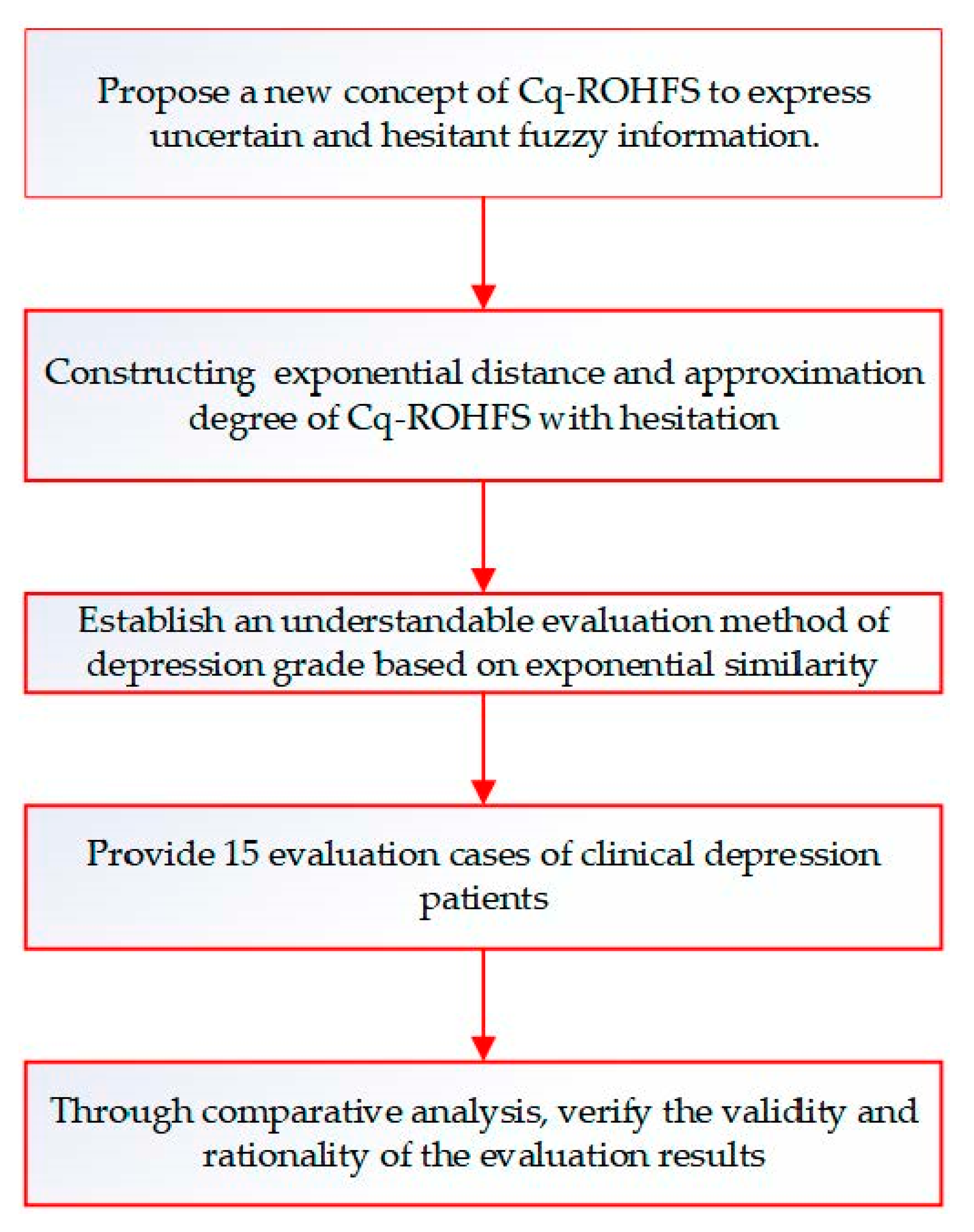
To show this study clearly, a flow chart is shown in Figure 1.

2. Preliminaries

Here, we review some basic concepts related to CS, CHFS, and q-ROHFS.

Regarding a hybrid form of an interval valued fuzzy set (IVFS) and a fuzzy value, a (fuzzy) cubic set CS is presented in a fixed non-empty set $\Delta$ by the following format [24]:

$$\mathrm{{\rm I}}=\left\{\langle \mathrm{u},\tilde{\vartheta }(u),\mu (u)\rangle |u\in \Delta \right\}$$

(1)

where $\tilde{\vartheta }(u)=[{\vartheta }^{-}(u),{\vartheta }^{+}(u)]$ is an IVFS, $\mu (u)$ is a fuzzy value.

Considering a hybrid form of both an interval valued hesitant fuzzy set (IVHFS) and a hesitant fuzzy set (HFS), a cubic hesitant fuzzy set (CHFS) is defined below.

Definition 1.

Set $\Delta$ as a fixed non-empty set. A CHFS $R$ is defined as the following form [43]:

$$E=\left\{\langle r_s,{\tilde{\vartheta }}_E(r_s),{\tilde{h}}_E(r_s)\rangle |r_s\in \Delta \right\}$$

(2)

where ${\tilde{\vartheta }}_E(r_s)$ is an interval valued hesitant fuzzy set for ${\tilde{\vartheta }}_E(r_s)=[{\vartheta }^{-}(r_s),{\vartheta }^{+}(r_s)]\subseteq [0,1]$, and ${\tilde{h}}_E(r_s)$ for $r_s\in \Delta$ is a HFS, which contains several different fuzzy values in $[0,1]$ expressed by ${\tilde{h}}_E(r_s)=\left\{{\mu }_1,{\mu }_2,\dots ,,{\mu }_t\right\}$ in ascending order.

Then, the fundamental element $\langle r_s,{\tilde{\vartheta }}_E(r_s),{\tilde{h}}_E(r_s)\rangle$ in Δ $$denoted simply as $e=\langle \tilde{\vartheta },\tilde{h}\rangle$, for the sake of convenience, is called a cubic hesitant fuzzy element (CHFE).

Definition 2.

Let$\Delta =\{r_2,r_2,\dots ,r_n\}$be the universe,

$$Q=\left\{{\langle r_s,\left(h_Q(r_s),g_Q(r_s)\right)\rangle }_q|r_s\in \Delta \right\}$$

(3)

where$q\ge 1$be the q-rung orthopair hesitant fuzzy set (q-ROHFS) on$\Delta$, $h_Q(r_s),g_Q(r_s)$represent all possible q-rung orthopair membership degrees and q-rung orthopair non-membership degrees of$r_s$belonging$Q$composition collection [44]. Where ${\mu }_Q\in h_Q(r_s)$, ${\nu }_Q\in g_Q(r_s)$, then satisfies $0\le {\mu }_Q(r_s),{\nu }_Q(r_s)\le 1,$ $0\le \sup {({\mu }_Q(r_{sj}))}^q+\sup {({\nu }_Q(r_{sj}))}^q\le 1,\left(q\ge 1\right)$ in an ascending order.

Definition 3.

Let$\Delta$be a non-empty set,

$$\stackrel{⌣}{Q}=\left\{\langle r_s,{\mu }_{\stackrel{⌣}{Q}}(r_s),{\upsilon }_{\stackrel{⌣}{Q}}(r_s)|r_s\in \Delta \rangle \right\}$$

(4)

is called an interval valued q-rung orthopair hesitant fuzzy set (IVq-ROHFS) on$\Delta$. Among them,${\mu }_{\stackrel{⌣}{Q}}(r_{sj})=[{\varsigma }_{\stackrel{⌣}{Q}}^{-}(r_{sj}),{\varsigma }_{\stackrel{⌣}{Q}}^{+}(r_{sj})]$, ${\upsilon }_{\stackrel{⌣}{Q}}(r_s)=\left[{\delta }_{\stackrel{⌣}{Q}}^{-}(r_{sj}),{\delta }_{\stackrel{⌣}{Q}}^{+}(r_{sj})\right]$are defined as all possible membership function and non-membership function to which the element$r_s$belong$\Delta$, and$r_s\in \Delta$, $q\ge 1$, $\left[{\varsigma }_{\stackrel{⌣}{Q}}^{-}(r_{sj}),{\varsigma }_{\stackrel{⌣}{Q}}^{+}(r_{sj})\right]\in \left[0,1\right]$, $[{\delta }_{\stackrel{⌣}{Q}}^{-}(r_{sj}),$${\delta }_{\stackrel{⌣}{Q}}^{+}(r_{sj})]\in \left[0,1\right]$, $0\le \sup {\left({\varsigma }_{{}_{\stackrel{⌣}{Q}}}^{+}(r_{sj})\right)}^q+\sup {\left({\delta }_{{}_{\stackrel{⌣}{Q}}}^{+}(r_{sj})\right)}^q$$\le 1$.

By combining IVq-ROHFS and q-ROHFS, we defined the cubic q-rung orthopair hesitant fuzzy set in the following manner:

Definition 4.

Let Δ be a finite universe. The cubic q-rung orthopair hesitant fuzzy set$\Im$on the universe Δ is defined as

$$\Im =\left\{{\langle r_s,{\tilde{\vartheta }}_{\Im }(r_s),{\tilde{t}}_{\Im }(r_s)\rangle }_q|r_s\in \Delta \right\}(q\ge 1)$$

(5)

where${\tilde{\vartheta }}_{\Im }(r_s):\Delta \to [0,1]$is an IVq-ROHFS${\tilde{\vartheta }}_{\Im }(r_s)=\left({\tilde{\mu }}_{\Im }(r_s),{\tilde{\upsilon }}_{\Im }(r_s)\right)$on$\Delta$and${\tilde{t}}_{\Im }(r_s):$ $\Delta \to [0,1]$is a q-ROHFS${\tilde{t}}_{\Im }(r_s)=\left(h_{\Im }(r_s),g_{\Im }(r_s)\right)$on$\Delta$.

A cubic q-rung orthopair hesitant fuzzy number (Cq-ROHFN) can be expressed as

$${\Im }_s=\langle \begin{array}{l}\left\{\left[{\varsigma }_{\Im }^{-}(r_{s1}),{\varsigma }_{\Im }^{+}(r_{s1})\right],\left[{\varsigma }_{\Im }^{-}(r_{s2}),{\varsigma }_{\Im }^{+}(r_{s2})\right],\dots ,\left[{\varsigma }_{\Im }^{-}(r_{sl(\tilde{\mu }{r}_s)}),{\varsigma }_{\Im }^{+}(r_{sl(\tilde{\mu }{r}_s)})\right]\right\},\\ \left\{\left[{\delta }_{\Im }^{-}(r_{s1}),{\delta }_{\Im }^{+}(r_{s1})\right],\left[{\delta }_{\Im }^{-}(r_{s2}),{\delta }_{\Im }^{+}(r_{s2})\right],\dots ,\left[{\delta }_{\Im }^{-}(r_{sl(\tilde{\mu }{r}_s)}),{\delta }_{\Im }^{+}(r_{sl(\tilde{\mu }{r}_s)})\right]\right\},\\ \left\{{\phi }_{\Im }(r_{s1}),{\phi }_{\Im }(r_{s2}),\dots ,{\phi }_{\Im }(r_{sl(h{r}_s)})\right\},\left\{{\psi }_{\Im }(r_{s1}),{\psi }_{\Im }(r_{s2}),\dots ,{\psi }_{\Im }(r_{sl(g{r}_s)})\right\}\end{array}\rangle$$

(6)

and abbreviated as $\langle {\tilde{\vartheta }}_s,{\tilde{t}}_s\rangle =\langle \left({\tilde{\mu }}_{\Im }(r_s),{\tilde{\upsilon }}_{\Im }(r_s)\right),(h_{\Im }(r_s),g_{\Im }(r_s))\rangle$.

For simplicity, an IVq-ROHFN and a q-ROHFN construct $\left({\tilde{\mu }}_{\Im }(r_s),{\tilde{\upsilon }}_{\Im }(r_s)\right)$ the Cq-ROHFN $\left(h_{\Im }(r_s),g_{\Im }(r_s)\right)$. When $q=1$, then ${\Im }_s$ is a cubic intuition hesitant fuzzy number (CIHFN) when $q=2$, then ${\Im }_s$ is a cubic Pythagorean hesitant fuzzy number (CPHFN), and when $q=3$, then ${\Im }_s$ is a cubic Fermatean hesitant fuzzy number (CFHFN).

Therefore, a Cq-ROHFS consists of a hybrid set that is made up of both an IVq-ROHFS and a q-ROHFS. The Cq-ROHFS offer the advantage that they can hold a great deal more information for representing the IVq-ROHFS and q-ROHFS simultaneously.

Definition 5.

Set,

$$\begin{array}{l}{\Im }_s=\langle {\tilde{\vartheta }}_{\Im }(r_s),{\tilde{t}}_{\Im }(r_s)\rangle =\langle \left\{{\tilde{\mu }}_{\Im }(r_s),{\tilde{\upsilon }}_{\Im }(r_s)\right\},\left\{h_{\Im }(r_s),g_{\Im }(r_s)\right\}\rangle \\ =\langle \begin{array}{l}\left\{\left[{\varsigma }_{\Im }^{-}(r_{s1}),{\varsigma }_{\Im }^{+}(r_{s1})\right],\left[{\varsigma }_{\Im }^{-}(r_{s2}),{\varsigma }_{\Im }^{+}(r_{s2})\right],\dots ,\left[{\varsigma }_{\Im }^{-}(r_{sl(\tilde{\mu }{r}_s)}),{\varsigma }_{\Im }^{+}(r_{sl(\tilde{\mu }{r}_s)})\right]\right\},\\ \left\{\left[{\delta }_{\Im }^{-}(r_{s1}),{\delta }_{\Im }^{+}(r_{s1})\right],\left[{\delta }_{\Im }^{-}(r_{s2}),{\delta }_{\Im }^{+}(r_{s2})\right],\dots ,\left[{\delta }_{\Im }^{-}(r_{sl(\tilde{\mu }{r}_s)}),{\delta }_{\Im }^{+}(r_{sl(\tilde{\mu }{r}_s)})\right]\right\},\\ \left\{{\phi }_{\Im }(r_{s1}),{\phi }_{\Im }(r_{s2}),\dots ,{\phi }_{\Im }(r_{sl(h{r}_s)})\right\},\left\{{\psi }_{\Im }(r_{s1}),{\psi }_{\Im }(r_{s2}),\dots ,{\psi }_{\Im }(r_{sl(g{r}_s)})\right\}\end{array}\rangle \end{array}$$

as a Cq-ROHFN, then call it:

• Membership-internal (briefly, M-Internal) if the following inequality holds:

$$\min \left({\varsigma }_{\Im }^{-}(r_s)\right)\le {\phi }_{\Im }(r_s)\le \max \left({\varsigma }_{\Im }^{+}(r_s)\right)$$

(7)

2.

Non-membership-internal (briefly, N-Internal) if the following inequality is valid:

$$\min \left({\delta }_{\Im }^{-}(r_s)\right)\le {\psi }_{\Im }(r_s)\le \max \left({\delta }_{\Im }^{+}(r_s)\right)$$

(8)

If a Cq-ROHFN in$\Delta$satisfies (7) and (8) for$s=1,2,\dots n$, $r_s\in \Delta$, we say that ${\Im }_s$ is an internal Cq-ROHFN.

For instance, ${\Im }_1=\langle {\tilde{\vartheta }}_{\Im }(r_1),{\tilde{t}}_{\Im }(r_1)\rangle =\langle \left\{\left[0.3,0.8\right]\right\},\left\{\left[0.4,0.9\right]\right\},\left\{0.3,0.4,0.7\right\},\{0.5,0.8\}\rangle$is an internal Cq-ROHFN, where $\langle \left\{\left[0.3,0.8\right]\right\},\left\{\left[0.4,0.9\right]\right\}\rangle$is its IVq-ROHFN and $\langle \left\{0,3,0,4,0,7\right\},\left\{0.5,0.8\right\}\rangle$ is its q-ROHFN.

Definition 6.

Set,

$${\Im }_1=\langle \left\{{\tilde{\mu }}_{\Im }(r_1),{\tilde{\upsilon }}_{\Im }(r_1)\right\},\left\{h_{\Im }(r_1),g_{\Im }(r_1)\right\}\rangle =\langle \begin{array}{l}\left\{\left[{\varsigma }_{\Im }^{-}(r_{11}),{\varsigma }_{\Im }^{+}(r_{11})\right],\left[{\varsigma }_{\Im }^{-}(r_{12}),{\varsigma }_{\Im }^{+}(r_{12})\right],\dots ,\left[{\varsigma }_{\Im }^{-}(r_{1l(\tilde{\mu }{r}_s)}),{\varsigma }_{\Im }^{+}(r_{1l(\tilde{\mu }{r}_s)})\right]\right\},\\ \left\{\left[{\delta }_{\Im }^{-}(r_{11}),{\delta }_{\Im }^{+}(r_{11})\right],\left[{\delta }_{\Im }^{-}(r_{12}),{\delta }_{\Im }^{+}(r_{12})\right],\dots ,\left[{\delta }_{\Im }^{-}(r_{1l(\tilde{\mu }{r}_s)}),{\delta }_{\Im }^{+}(r_{1l(\tilde{\mu }{r}_s)})\right]\right\},\\ \left\{{\phi }_{\Im }(r_{11}),{\phi }_{\Im }(r_{12}),\dots ,{\phi }_{\Im }(r_{1l(h{r}_s)})\right\},\left\{{\psi }_{\Im }(r_{11}),{\psi }_{\Im }(r_{12}),\dots ,{\psi }_{\Im }(r_{1l(g{r}_s)})\right\}\end{array}\rangle ,$$

and,

$${\Im }_2=\langle \left\{{\tilde{\mu }}_{\Im }(r_2),{\tilde{\upsilon }}_{\Im }(r_2)\right\},\left\{h_{\Im }(r_2),g_{\Im }(r_2)\right\}\rangle =\langle \begin{array}{l}\left\{\left[{\varsigma }_{\Im }^{-}(r_{21}),{\varsigma }_{\Im }^{+}(r_{21})\right],\left[{\varsigma }_{\Im }^{-}(r_{22}),{\varsigma }_{\Im }^{+}(r_{22})\right],\dots ,\left[{\varsigma }_{\Im }^{-}(r_{2l(\tilde{\mu }{r}_s)}),{\varsigma }_{\Im }^{+}(r_{2l(\tilde{\mu }{r}_s)})\right]\right\},\\ \left\{\left[{\delta }_{\Im }^{-}(r_{21}),{\delta }_{\Im }^{+}(r_{21})\right],\left[{\delta }_{\Im }^{-}(r_{22}),{\delta }_{\Im }^{+}(r_{22})\right],\dots ,\left[{\delta }_{\Im }^{-}(r_{2l(\tilde{\mu }{r}_s)}),{\delta }_{\Im }^{+}(r_{2l(\tilde{\mu }{r}_s)})\right]\right\},\\ \left\{{\phi }_{\Im }(r_{21}),{\phi }_{\Im }(r_{22}),\dots ,{\phi }_{\Im }(r_{2l(h{r}_s)})\right\},\left\{{\psi }_{\Im }(r_{21}),{\psi }_{\Im }(r_{22}),\dots ,{\psi }_{\Im }(r_{2l(g{r}_s)})\right\}\end{array}\rangle$$

as two Cq-ROHFs, then their relations are defined as follows:

• If ${\Im }_1={\Im }_2$, then ${\tilde{\vartheta }}_{\Im }(r_1)={\tilde{\vartheta }}_{\Im }(r_2)$, and ${\tilde{t}}_{\Im }(r_1)={\tilde{t}}_{\Im }(r_2)$, i.e., ${\varsigma }_{\Im }^{-(\iota )}(r_1)={\varsigma }_{\Im }^{-(\iota )}(r_2)$, ${\varsigma }_{\Im }^{+(\iota )}(r_1)={\varsigma }_{\Im }^{+(\iota )}(r_2)$, ${\delta }_{\Im }^{-(\sigma )}(r_1)={\delta }_{\Im }^{-(\sigma )}(r_2)$, ${\delta }_{\Im }^{+(\sigma )}(r_1)={\delta }_{\Im }^{+(\sigma )}(r_2)$, and ${\phi }_{\Im }^{(m)}(r_1)={\phi }_{\Im }^{(m)}(r_2)$, ${\psi }_{\Im }^{(n)}(r_1)={\psi }_{\Im }^{(n)}(r_2)$, for $\iota =1,2,\dots ,l(\tilde{\mu }{r}_s)$, $\sigma =1,2,\dots ,l(\tilde{\upsilon }{r}_s)$, $m=1,2,\dots ,l(h{r}_s)$, and $n=1,2,\dots ,l(g{r}_s)$;
• If ${\Im }_1\subseteq {\Im }_2$, then${\tilde{\vartheta }}_1\subseteq {\tilde{\vartheta }}_2$, and${\tilde{t}}_{1j}\subseteq {\tilde{t}}_{2j}$for$j=1,2,\dots n_s$.

3. Novel Distance and Similarity Measures

We introduce the hesitance degree concept before developing some novel distance measures using Cq-ROHFS. Following the definition of the hesitance degree on the hesitant fuzzy set [45], the hesitance degree on Cq-ROHFS is defined as follows:

Definition 7.

Let ${\tilde{\mu }}_{\Im }$, $h_{\Im }$ and ${\tilde{\upsilon }}_{\Im }$, $g_{\Im }$. be a set of all possible q-rung orthopair membership and q-rung orthopair non-membership that $r_{sj}$ belongs to $\Im$, respectively. Their respective lengths are $l({\tilde{\mu }}_{\Im })$, $l(h_{\Im })$, $l({\tilde{\upsilon }}_{\Im })$ and $l(g_{\Im }(r_s))$. Their degrees of hesitation are defined as follows: 

$$u({\tilde{\mu }}_{\Im })=1-\frac{1}{l({\tilde{\mu }}_{\Im })}, u(h_{\Im })=1-\frac{1}{l(h_{\Im })}, u({\tilde{\upsilon }}_{\Im })=1-\frac{1}{l({\tilde{\upsilon }}_{\Im })}, \mathrm{and} u(g_{\Im })=1-\frac{1}{l(g_{\Im })}$$

For any cubic q-rung orthopair hesitation fuzzy elements, the values of $u({\tilde{\mu }}_{\Im })$, $u(h_{\Im })$, $u({\tilde{\upsilon }}_{\Im }(r_s))$, and $u(g_{\Im })$ reflect the degree of hesitation of decision makers in determining the membership and non-membership of ${\vartheta }_{\Im }$ and $t_{\Im }$. The greater the value, the more hesitant the decision maker will be.

For example, if $l({\tilde{\mu }}_{\Im })=1$, $l({\tilde{\upsilon }}_{\Im })=1$, $l(h_{\Im })=1$, and $l(g_{\Im })=1$, then we have $u({\tilde{\mu }}_{\Im })=0$, $u({\tilde{\upsilon }}_{\Im })=0$, $u(h_{\Im })=0$, and $u(g_{\Im })=0$. In other words, this implies that the decision maker is confident in determining the membership’s exact value. As a consequence, decision makers do not hesitate to assess the value of membership.

It should be noted, however, that if $l({\tilde{\mu }}_{\Im })$, $l(h_{\Im })$, $l({\tilde{\upsilon }}_{\Im })$ and $l(g_{\Im })$ tend to infinity, then we have $u({\tilde{\mu }}_{\Im })=1$, $u({\tilde{\upsilon }}_{\Im })=1$, $u(h_{\Im })=1$, $u(g_{\Im })=1$, which indicate that the decision maker is indecisive and unable to assess the value of membership. If decision makers hesitate when evaluating an alternative or indicator, $u({\tilde{\mu }}_{\Im })$, $u({\tilde{\upsilon }}_{\Im })$, $u(h_{\Im })$ and $u(g_{\Im })$ show the degree of hesitancy.

Among several Cq-ROHFSs, $0\le u({\tilde{\mu }}_{\Im })\le 1$, $0\le u({\tilde{\upsilon }}_{\Im })\le 1$, $0\le u(h_{\Im })\le 1$ and $0\le u(g_{\Im })\le 1$, the larger the values of $u({\tilde{\mu }}_{\Im })$, $u({\tilde{\upsilon }}_{\Im })$, $u(h_{\Im })$ and $u(g_{\Im })$, the more hesitant the decision makers.

Let $u({\tilde{\mu }}_{\Im })=0$, $u({\tilde{\upsilon }}_{\Im })=0$, $u(h_{\Im })=0$, $u(g_{\Im })=0$; this means that the decision maker has no hesitancy in determining the importance of Cq-ROHFSs. When $u({\tilde{\mu }}_{\Im })\to 1$, $u({\tilde{\upsilon }}_{\Im })\to 1$, $u(h_{\Im })\to 1$, and $u(g_{\Im })\to 1$, it means that the decision maker finds it difficult to decide on the values of Cq-ROHFSs and is entirely hesitant.

Example 1.

Let${\Im }_1=\langle \left\{{\tilde{\mu }}_{\Im }(r_1),{\tilde{\upsilon }}_{\Im }(r_1)\right\},\left\{h_{\Im }(r_1),g_{\Im }(r_1)\right\}\rangle =\langle \{\left[0.2,0.5\right],\left[0.4,0.6\right]\},\left\{\left[0.3,0.8\right]\right\},$ $\{0.2,0.7,0.9\},\left\{0.4,0.6\right\}\rangle$, it means${\tilde{\mu }}_{\Im }(r_1)=\left\{[0.2,0.5],[0.4,0.6]\right\}$, ${\tilde{\upsilon }}_{\Im }(r_1)=\left\{\left[0.3,0.8\right]\right\}$, and$h_{\Im }(r_1)=\{0.2,0.7,0.9\}$, $g_{\Im }(r_1)=\left\{0.4,0.6\right\}$, then we have the degree of hesitancy as follows:

$$\begin{gathered} u({\tilde{\mu }}_{\Im }(r_1))=1-\frac{1}{2}=\frac{1}{2}, u({\tilde{\upsilon }}_{\Im }(r_1))=1-1=0, and u(h_{\Im }(r_1))=1-\frac{1}{3}=\frac{2}{3}, \\ u(g_{\Im }(r_1))=1-\frac{1}{2}=\frac{1}{2}. \end{gathered}$$

There may be a discrepancy in the number of elements in the hesitant fuzzy set due to incomplete decision information provided by decision makers or for other reasons. As in Cq-ROHFs, decision makers with different mindsets have different attitudes towards a given decision. This problem can be solved using the least common multiple expansion method in order to reduce the error caused by subjective factors.

Definition 8.

Since, in general, the lengths of the q-rung orthopair hesitant fuzzy elements in${\Im }_A$and${\Im }_B$, namely$l({\tilde{\mu }}_{\Im })$, $l(h_{\Im })$, $l({\tilde{\upsilon }}_{\Im })$and$l(g_{\Im })$, are not equal, suppose there are n q-rung orthopair hesitation fuzzy elements${\tilde{\vartheta }}_{\Im }$and${\tilde{t}}_{\Im }$, which do not have the same number of membership and non-membership degrees. Let${\ell }_S$, $M_S$and${\rho }_S$, $N_S$be the least common multiple of the number of possible membership and non-membership elements [46], that means ${\ell }_s=[l\left({\tilde{\mu }}_{{\Im }_A}\right),l\left({\tilde{\mu }}_{{\Im }_B}\right)]$, ${\rho }_s=[l\left({\tilde{\mu }}_{{\Im }_A}\right),l\left({\tilde{\mu }}_{{\Im }_B}\right)]$, $M_s=[l\left(h_{{\Im }_A}\right),$$l\left(h_{{\Im }_B}\right)]$, $N_s=[l\left(g_{{\Im }_A}\right),$$l\left(g_{{\Im }_B}\right)]$.

If all elements in $h_{{\Im }_A}$, $h_{{\Im }_B}$ are duplicated $\frac{M_s}{l(h_{{\Im }_B})}$, $\frac{M_s}{l(h_{{\Im }_A})}$ times, and all elements in $g_{{\Im }_A}$ and $g_{{\Im }_B}$ are repeated $\frac{N_s}{l(g_{{\Im }_B})}$, $\frac{N_s}{l(g_{{\Im }_A})}$ times in an ascending order, the LCM expansion method of elements in ${\tilde{\vartheta }}_{\Im }(r_s)$ are the same. Then, the number of elements in all Cq-ROHFSs is equal.

Example 2.

For example, suppose ${\Im }_1^{\text{'}}=\langle \left\{\left[0.2,0.5\right],\left[0.1,0.4\right]\right\},\left\{\left[0.2,0.3\right]\right\},\{0.3,0.4,$$0.6\},\left\{0.7\right\}\rangle$ and ${\Im }_2^{\text{'}}=\langle \left\{\left[0.4,0.6\right]\right\},\left\{\left[0.1,0.5\right],\left[0.3,0.4\right]\right\},\left\{0.2,0.7\right\},\{0.1,0.5,0.8\}$. are two Cq-ROHFSs. Then, we obtain their least common multiple numbers (LCMN) ${\ell }_s=2$, ${\rho }_s=2$, $M_s=6$ and $N_s=3$ in ${\Im }_1^{\text{'}}$ and ${\Im }_2^{\text{'}}$. Based on Definition 7, the two Cq-ROHFSs ${\Im }_1^{\text{'}}$ and ${\Im }_2^{\text{'}}$ can be extended to the following forms: 

$$\begin{gathered} {\Im }^{\text{'}}{}_1=\langle \left\{\left[0.2,0.5\right],\left[0.1,0.4\right]\right\},\left\{\left[0.2,0.3\right],\left[0.2,0.3\right]\right\},\left\{0.3,0.3,0.4,0.4,0.6,0.6\right\},\left\{0.7,0.7,0.7\right\}\rangle , \\ {\Im }^{\text{'}}{}_2=\langle \left\{\left[0.4,0.6\right],\left[0.4,0.6\right]\right\},\left\{\left[0.1,0.5\right],\left[0.3,0.4\right]\right\},\left\{0.2,0.2,0.2,0.7,0.7,0.7\right\},\left\{0.1,0.5,0.8\right\}\rangle . \end{gathered}$$

3.1. Novel Exponential Distance Measures between Cq-ROHFSs

In this section, we extend the exponential distance to the q-rung orthopair hesitant setting, and formulate an exponential distance with hesitancy based on Cq-ROHFSs.

Definition 9.

Inspired by [45,46,47], let ${\Im }_A$ and ${\Im }_B$ be two Cq-ROHFSs on the universal set $\Delta$, where ${\varsigma }_{{\Im }_A}^{-(\iota )}(r_s)$, ${\varsigma }_{{\Im }_A}^{+(\iota )}(r_s)$ and ${\varsigma }_{{\Im }_B}^{-(\iota )}(r_s)$, ${\varsigma }_{{\Im }_B}^{+(\iota )}(r_s)$, are the $\iota -th$ largest values in 

${\tilde{\mu }}_{{\Im }_A}(r_s)$,${\tilde{\mu }}_{{\Im }_B}(r_s)$; then ${\phi }_{{\Im }_A}^{(m)}(r_s)$ and ${\phi }_{{\Im }_B}^{(m)}(r_s)$ are the $m-th$ largest values in $h_{{\Im }_A}(r_s)$, $h_{{\Im }_B}(r_s)$, respectively. Other elements are the same, and used thereafter. The exponential distance between ${\Im }_A$ and ${\Im }_B$ are defined as follows:

$$d_{eg}(A,B)=\frac{1-\exp \left\{-{\left[{\displaystyle \sum _{s=1}^n\frac{1}{{\ell }_s+{{\rm M}}_s+{\rho }_s+N_s+4}}\left(\begin{array}{l}\left({\left|u({\tilde{\mu }}_{{\Im }_A}(r_s))-u({\tilde{\mu }}_{{\Im }_B}(r_s))\right|}^q+{\left|u(h_{{\Im }_A}(r_s))-u(h_{{\Im }_B}(r_s))\right|}^q\right)\\ +\left({\displaystyle \sum _{\iota =1}^{{\ell }_s}\left({\left|{\varsigma }_{{\Im }_A}^{-(\iota )}(r_s)-{\varsigma }_{{\Im }_B}^{-(\iota )}(r_s)\right|}^q+{\left|{\varsigma }_{{\Im }_A}^{+(\iota )}(r_s)-{\varsigma }_{{\Im }_B}^{+(\iota )}(r_s)\right|}^q\right)}+{\displaystyle \sum _{m=1}^{{{\rm M}}_s}{\left|{\phi }_{{\Im }_A}^{(m)}(r_s)-{\phi }_{{\Im }_B}^{(m)}(r_s)\right|}^q}\right)\\ +\left({\left|u({\tilde{\upsilon }}_{{\Im }_A}(r_s))-u({\tilde{\upsilon }}_{{\Im }_B}(r_s))\right|}^q+{\left|u(g_{{\Im }_A}(r_s))-u(g_{{\Im }_B}(r_s))\right|}^q\right)\\ +\left({\displaystyle \sum _{\sigma =1}^{{\rho }_s}\left({\left|{\delta }_{{\Im }_A}^{-(\sigma )}(r_s)-{\delta }_{{\Im }_B}^{-(\sigma )}(r_s)\right|}^q+{\left|{\delta }_{{\Im }_A}^{+(\sigma )}(r_s)-{\delta }_{{\Im }_B}^{+(\sigma )}(r_s)\right|}^q\right)}+{\displaystyle \sum _{n=1}^{N_s}{\left|{\psi }_{{\Im }_A}^{(n)}(r_s)-{\psi }_{{\Im }_B}^{(n)}(r_s)\right|}^q}\right)\end{array}\right)\right]}^{1/q}\right\}}{1-\exp \left(-{\left(n\right)}^{1/q}\right)}$$

(9)

During the actual decision-making process, the decision makers may have a different preference between the hesitance degree and the values of Cq-ROHFSs. Accordingly, the distance measure with preference information on Cq-ROHFSs is defined as follows:

$$d_{epg}(A,B)=\frac{1-\exp \left\{-{\left[{\displaystyle \sum _{s=1}^n\frac{1}{{\ell }_s+{{\rm M}}_s+{\rho }_s+N_s+4}}\left(\begin{array}{l}\alpha \left({\left|u({\tilde{\mu }}_{{\Im }_A}(r_s))-u({\tilde{\mu }}_{{\Im }_B}(r_s))\right|}^q+{\left|u(h_{{\Im }_A}(r_s))-u(h_{{\Im }_B}(r_s))\right|}^q\right)\\ +\beta \left({\displaystyle \sum _{\iota =1}^{{\ell }_s}\left({\left|{\varsigma }_{{\Im }_A}^{-(\iota )}(r_s)-{\varsigma }_{{\Im }_B}^{-(\iota )}(r_s)\right|}^q+{\left|{\varsigma }_{{\Im }_A}^{+(\iota )}(r_s)-{\varsigma }_{{\Im }_B}^{+(\iota )}(r_s)\right|}^q\right)}+{\displaystyle \sum _{m=1}^{{{\rm M}}_s}{\left|{\phi }_{{\Im }_A}^{(m)}(r_s)-{\phi }_{{\Im }_B}^{(m)}(r_s)\right|}^q}\right)\\ +\gamma \left({\left|u({\tilde{\upsilon }}_{{\Im }_A}(r_s))-u({\tilde{\upsilon }}_{{\Im }_B}(r_s))\right|}^q+{\left|u(g_{{\Im }_A}(r_s))-u(g_{{\Im }_B}(r_s))\right|}^q\right)\\ +\eta \left({\displaystyle \sum _{\sigma =1}^{{\rho }_s}\left({\left|{\delta }_{{\Im }_A}^{-(\sigma )}(r_s)-{\delta }_{{\Im }_B}^{-(\sigma )}(r_s)\right|}^q+{\left|{\delta }_{{\Im }_A}^{+(\sigma )}(r_s)-{\delta }_{{\Im }_B}^{+(\sigma )}(r_s)\right|}^q\right)}+{\displaystyle \sum _{n=1}^{N_s}{\left|{\psi }_{{\Im }_A}^{(n)}(r_s)-{\psi }_{{\Im }_B}^{(n)}(r_s)\right|}^q}\right)\end{array}\right)\right]}^{1/q}\right\}}{1-\exp \left(-{\left(n\right)}^{1/q}\right)}$$

(10)

where $\alpha ,\beta ,\gamma ,\eta \in \left[0,1\right]$, $\alpha +\beta =1,\gamma +\eta =1$.

As $\alpha ,\gamma$ changes, distance results also change, which means that the degree of hesitation influences the final decision. In particular, when $\alpha ,\gamma$ increases, for example $\alpha =\gamma =0.8$, we tend to focus more on the differences between hesitations rather than the differences between values. This is because the differences between hesitations have a stronger effect than the differences between values, and this effect is sufficient to compensate for the differences between values.

Nevertheless, there are several practical problems in which parameter weights play an important role in decision making. In some cases, each element may have a different substantial degree, so distance measures for Cq-ROHFS should take the weight of the component into account. Let us consider the weight $W={(w_1,w_2,\dots ,w_n)}^T$ of each element $r_s\in \Delta$, with a distinction between hesitation and membership/non-membership values. A weighted exponential distance measure with preference is defined as follows:

$$d_{ewpg}(A,B)=\frac{1-\exp \left\{-{\left[{\displaystyle \sum _{s=1}^n\frac{w_s}{{\ell }_s+{{\rm M}}_s+{\rho }_s+N_s+4}}\left(\begin{array}{l}\alpha \left({\left|u({\tilde{\mu }}_{{\Im }_A}(r_s))-u({\tilde{\mu }}_{{\Im }_B}(r_s))\right|}^q+{\left|u(h_{{\Im }_A}(r_s))-u(h_{{\Im }_B}(r_s))\right|}^q\right)\\ +\beta \left({\displaystyle \sum _{\iota =1}^{{\ell }_s}\left({\left|{\varsigma }_{{\Im }_A}^{-(\iota )}(r_s)-{\varsigma }_{{\Im }_B}^{-(\iota )}(r_s)\right|}^q+{\left|{\varsigma }_{{\Im }_A}^{+(\iota )}(r_s)-{\varsigma }_{{\Im }_B}^{+(\iota )}(r_s)\right|}^q\right)}+{\displaystyle \sum _{m=1}^{{{\rm M}}_s}{\left|{\phi }_{{\Im }_A}^{(m)}(r_s)-{\phi }_{{\Im }_B}^{(m)}(r_s)\right|}^q}\right)\\ +\gamma \left({\left|u({\tilde{\upsilon }}_{{\Im }_A}(r_s))-u({\tilde{\upsilon }}_{{\Im }_B}(r_s))\right|}^q+{\left|u(g_{{\Im }_A}(r_s))-u(g_{{\Im }_B}(r_s))\right|}^q\right)\\ +\eta \left({\displaystyle \sum _{\sigma =1}^{{\rho }_s}\left({\left|{\delta }_{{\Im }_A}^{-(\sigma )}(r_s)-{\delta }_{{\Im }_B}^{-(\sigma )}(r_s)\right|}^q+{\left|{\delta }_{{\Im }_A}^{+(\sigma )}(r_s)-{\delta }_{{\Im }_B}^{+(\sigma )}(r_s)\right|}^q\right)}+{\displaystyle \sum _{n=1}^{N_s}{\left|{\psi }_{{\Im }_A}^{(n)}(r_s)-{\psi }_{{\Im }_B}^{(n)}(r_s)\right|}^q}\right)\end{array}\right)\right]}^{1/q}\right\}}{1-\exp \left(-{\left(n\right)}^{1/q}\right)}$$

(11)

Let $w_s\in \left[0,1\right]$, ${\displaystyle \sum _{s=1}^n{w}_s}=1$, $q>0$, and $\alpha ,\beta ,\lambda ,\eta \in \left[0,1\right]$, $\alpha +\beta =1,\lambda +\eta =1$. If $w={(\frac{1}{n},\frac{1}{n},\dots ,\frac{1}{n})}^T$; then, the distance measures $d_{ewpg}$ will become $d_{epg}$.

Theorem 1.

Let$A,B,C$be the three Cq-ROHFSs defined over the universal set$\Delta$; then the distance measures$d_{eg}(A,B)$, $d_{epg}(A,B)$satisfy the following properties.

• $d(A,B)\in \left[0,1\right]$;
• $d(A,B)=0$, if $A=B$;
• $d(A,B)=d(B,A)$.

Proof of Theorem 1.

Let $A$, $B$ and $C$ be three Cq-ROHFSs over the universal set $\Delta$; then, we have:

(P1) It is clear that $d(A,B)\ge 0$, so we need prove only $d(A,B)\le 1$. Since $A$ and $B$ are Cq-ROHFs, so we get ${\left|{\varsigma }_{{\Im }_A}^{-(\iota )}(r_s)-{\varsigma }_{{\Im }_B}^{-(\iota )}(r_s)\right|}^q\in \left[0,1\right]$, ${\left|{\varsigma }_{{\Im }_A}^{+(\iota )}(r_s)-{\varsigma }_{{\Im }_B}^{+(\iota )}(r_s)\right|}^q\in \left[0,1\right]$, $|{\delta }_{{\Im }_A}^{-(\sigma )}(r_s)-{{\delta }_{{\Im }_B}^{-(\sigma )}(r_s)|}^q\in \left[0,1\right]$, ${\left|{\delta }_{{\Im }_A}^{+(\sigma )}(r_s)-{\delta }_{{\Im }_B}^{+(\sigma )}(r_s)\right|}^q\in \left[0,1\right]$, ${|u\left({\mu }_{{\Im }_A}(r_s)\right)-u\left({\mu }_{{\Im }_B}(r_s)\right)|}^q\in$$\left[0,1\right]$, ${|u\left({\upsilon }_{{\Im }_A}(r_s)\right)-u\left({\upsilon }_{{\Im }_B}(r_s)\right)|}^q\in \left[0,1\right]$, ${\left|u\left(h_{{\Im }_A}(r_s)\right)-u\left(h_{{\Im }_B}(r_s)\right)\right|}^q\in \left[0,1\right]$, $|u\left(g_{{\Im }_A}(r_s)\right)-$${u\left(g_{{\Im }_B}(r_s)\right)|}^q\in \left[0,1\right]$, ${\displaystyle \sum _{m=1}^{M_s}{\left|{\phi }_{{\Im }_A}^{(m)}(r_s)-{\phi }_{{\Im }_B}^{(m)}(r_s)\right|}^q}\in \left[0,1\right]$ and ${\displaystyle \sum _{n=1}^{N_s}{\left|{\psi }_{{\Im }_A}^{(n)}(r_s)-{\psi }_{{\Im }_B}^{(n)}(r_s)\right|}^q}\in \left[0,1\right]$ then $q>0$, and $\alpha ,\beta ,\lambda ,\eta$$\in \left[0,1\right]$, $\alpha +\beta =1,\lambda +\eta =1$.

Thus, we have:

$$\begin{gathered} \left[{\displaystyle \sum _{s=1}^n\frac{1}{{\ell }_s+{{\rm M}}_s+{\rho }_s+N_s+4}}{\left(\begin{array}{l}\alpha \left({\left|u({\tilde{\mu }}_{{\Im }_A}(r_s))-u({\tilde{\mu }}_{{\Im }_B}(r_s))\right|}^q+{\left|u(h_{{\Im }_A}(r_s))-u(h_{{\Im }_B}(r_s))\right|}^q\right)\\ +\beta \left({\displaystyle \sum _{\iota =1}^{{\ell }_s}\left({\left|{\varsigma }_{{\Im }_A}^{-(\iota )}(r_s)-{\varsigma }_{{\Im }_B}^{-(\iota )}(r_s)\right|}^q+{\left|{\varsigma }_{{\Im }_A}^{+(\iota )}(r_s)-{\varsigma }_{{\Im }_B}^{+(\iota )}(r_s)\right|}^q\right)}+{\displaystyle \sum _{m=1}^{{{\rm M}}_s}{\left|{\phi }_{{\Im }_A}^{(m)}(r_s)-{\phi }_{{\Im }_B}^{(m)}(r_s)\right|}^q}\right)\\ +\gamma \left({\left|u({\tilde{\upsilon }}_{{\Im }_A}(r_s))-u({\tilde{\upsilon }}_{{\Im }_B}(r_s))\right|}^q+{\left|u(g_{{\Im }_A}(r_s))-u(g_{{\Im }_B}(r_s))\right|}^q\right)\\ +\eta \left({\displaystyle \sum _{\sigma =1}^{{\rho }_s}\left({\left|{\delta }_{{\Im }_A}^{-(\sigma )}(r_s)-{\delta }_{{\Im }_B}^{-(\sigma )}(r_s)\right|}^q+{\left|{\delta }_{{\Im }_A}^{+(\sigma )}(r_s)-{\delta }_{{\Im }_B}^{+(\sigma )}(r_s)\right|}^q\right)}+{\displaystyle \sum _{n=1}^{N_s}{\left|{\psi }_{{\Im }_A}^{(n)}(r_s)-{\psi }_{{\Im }_B}^{(n)}(r_s)\right|}^q}\right)\end{array}\right)}^{1/q}\right]\le {\left(n\right)}^{1/q} \\ \Rightarrow \exp \left\{-{\left[{\displaystyle \sum _{s=1}^n\frac{1}{{\ell }_s+{{\rm M}}_s+{\rho }_s+N_s+4}}\left(\begin{array}{l}\alpha \left({\left|u({\tilde{\mu }}_{{\Im }_A}(r_s))-u({\tilde{\mu }}_{{\Im }_B}(r_s))\right|}^q+{\left|u(h_{{\Im }_A}(r_s))-u(h_{{\Im }_B}(r_s))\right|}^q\right)\\ +\beta \left({\displaystyle \sum _{\iota =1}^{{\ell }_s}\left({\left|{\varsigma }_{{\Im }_A}^{-(\iota )}(r_s)-{\varsigma }_{{\Im }_B}^{-(\iota )}(r_s)\right|}^q+{\left|{\varsigma }_{{\Im }_A}^{+(\iota )}(r_s)-{\varsigma }_{{\Im }_B}^{+(\iota )}(r_s)\right|}^q\right)}+{\displaystyle \sum _{m=1}^{{{\rm M}}_s}{\left|{\phi }_{{\Im }_A}^{(m)}(r_s)-{\phi }_{{\Im }_B}^{(m)}(r_s)\right|}^q}\right)\\ +\gamma \left({\left|u({\tilde{\upsilon }}_{{\Im }_A}(r_s))-u({\tilde{\upsilon }}_{{\Im }_B}(r_s))\right|}^q+{\left|u(g_{{\Im }_A}(r_s))-u(g_{{\Im }_B}(r_s))\right|}^q\right)\\ +\eta \left({\displaystyle \sum _{\sigma =1}^{{\rho }_s}\left({\left|{\delta }_{{\Im }_A}^{-(\sigma )}(r_s)-{\delta }_{{\Im }_B}^{-(\sigma )}(r_s)\right|}^q+{\left|{\delta }_{{\Im }_A}^{+(\sigma )}(r_s)-{\delta }_{{\Im }_B}^{+(\sigma )}(r_s)\right|}^q\right)}+{\displaystyle \sum _{n=1}^{N_s}{\left|{\psi }_{{\Im }_A}^{(n)}(r_s)-{\psi }_{{\Im }_B}^{(n)}(r_s)\right|}^q}\right)\end{array}\right)\right]}^{1/q}\right\}\ge \exp \left(-{\left(n\right)}^{1/q}\right) \\ \begin{array}{l}\Rightarrow 1-\exp \left\{-{\left[{\displaystyle \sum _{s=1}^n\frac{1}{{\ell }_s+{{\rm M}}_s+{\rho }_s+N_s+4}}\left(\begin{array}{l}\alpha \left({\left|u({\tilde{\mu }}_{{\Im }_A}(r_s))-u({\tilde{\mu }}_{{\Im }_B}(r_s))\right|}^q+{\left|u(h_{{\Im }_A}(r_s))-u(h_{{\Im }_B}(r_s))\right|}^q\right)\\ +\beta \left({\displaystyle \sum _{\iota =1}^{{\ell }_s}\left({\left|{\varsigma }_{{\Im }_A}^{-(\iota )}(r_s)-{\varsigma }_{{\Im }_B}^{-(\iota )}(r_s)\right|}^q+{\left|{\varsigma }_{{\Im }_A}^{+(\iota )}(r_s)-{\varsigma }_{{\Im }_B}^{+(\iota )}(r_s)\right|}^q\right)}+{\displaystyle \sum _{m=1}^{{{\rm M}}_s}{\left|{\phi }_{{\Im }_A}^{(m)}(r_s)-{\phi }_{{\Im }_B}^{(m)}(r_s)\right|}^q}\right)\\ +\gamma \left({\left|u({\tilde{\upsilon }}_{{\Im }_A}(r_s))-u({\tilde{\upsilon }}_{{\Im }_B}(r_s))\right|}^q+{\left|u(g_{{\Im }_A}(r_s))-u(g_{{\Im }_B}(r_s))\right|}^q\right)\\ +\eta \left({\displaystyle \sum _{\sigma =1}^{{\rho }_s}\left({\left|{\delta }_{{\Im }_A}^{-(\sigma )}(r_s)-{\delta }_{{\Im }_B}^{-(\sigma )}(r_s)\right|}^q+{\left|{\delta }_{{\Im }_A}^{+(\sigma )}(r_s)-{\delta }_{{\Im }_B}^{+(\sigma )}(r_s)\right|}^q\right)}+{\displaystyle \sum _{n=1}^{N_s}{\left|{\psi }_{{\Im }_A}^{(n)}(r_s)-{\psi }_{{\Im }_B}^{(n)}(r_s)\right|}^q}\right)\end{array}\right)\right]}^{1/q}\right\}\\ \le 1-\exp \left(-{\left(n\right)}^{1/q}\right)\end{array} \\ \Rightarrow \frac{1-\exp \left\{-{\left[{\displaystyle \sum _{s=1}^n\frac{1}{{\ell }_s+{{\rm M}}_s+{\rho }_s+N_s+4}}\left(\begin{array}{l}\alpha \left({\left|u({\tilde{\mu }}_{{\Im }_A}(r_s))-u({\tilde{\mu }}_{{\Im }_B}(r_s))\right|}^q+{\left|u(h_{{\Im }_A}(r_s))-u(h_{{\Im }_B}(r_s))\right|}^q\right)\\ +\beta \left({\displaystyle \sum _{\iota =1}^{{\ell }_s}\left({\left|{\varsigma }_{{\Im }_A}^{-(\iota )}(r_s)-{\varsigma }_{{\Im }_B}^{-(\iota )}(r_s)\right|}^q+{\left|{\varsigma }_{{\Im }_A}^{+(\iota )}(r_s)-{\varsigma }_{{\Im }_B}^{+(\iota )}(r_s)\right|}^q\right)}+{\displaystyle \sum _{m=1}^{{{\rm M}}_s}{\left|{\phi }_{{\Im }_A}^{(m)}(r_s)-{\phi }_{{\Im }_B}^{(m)}(r_s)\right|}^q}\right)\\ +\gamma \left({\left|u({\tilde{\upsilon }}_{{\Im }_A}(r_s))-u({\tilde{\upsilon }}_{{\Im }_B}(r_s))\right|}^q+{\left|u(g_{{\Im }_A}(r_s))-u(g_{{\Im }_B}(r_s))\right|}^q\right)\\ +\eta \left({\displaystyle \sum _{\sigma =1}^{{\rho }_s}\left({\left|{\delta }_{{\Im }_A}^{-(\sigma )}(r_s)-{\delta }_{{\Im }_B}^{-(\sigma )}(r_s)\right|}^q+{\left|{\delta }_{{\Im }_A}^{+(\sigma )}(r_s)-{\delta }_{{\Im }_B}^{+(\sigma )}(r_s)\right|}^q\right)}+{\displaystyle \sum _{n=1}^{N_s}{\left|{\psi }_{{\Im }_A}^{(n)}(r_s)-{\psi }_{{\Im }_B}^{(n)}(r_s)\right|}^q}\right)\end{array}\right)\right]}^{1/q}\right\}}{1-\exp \left(-{\left(n\right)}^{1/q}\right)}\le 1 \\ d(A,B)\le 1. \end{gathered}$$

(P2) For two Cq-ROHFSs $A$ and $B$, assume that $d(A,B)=0$; then:

$$\begin{gathered} \iff \exp \left\{-{\left[{\displaystyle \sum _{s=1}^n\frac{1}{{\ell }_s+{{\rm M}}_s+{\rho }_s+N_s+4}}\left(\begin{array}{l}\alpha \left({\left|u({\tilde{\mu }}_{{\Im }_A}(r_s))-u({\tilde{\mu }}_{{\Im }_B}(r_s))\right|}^q+{\left|u(h_{{\Im }_A}(r_s))-u(h_{{\Im }_B}(r_s))\right|}^q\right)\\ +\beta \left({\displaystyle \sum _{\iota =1}^{{\ell }_s}\left({\left|{\varsigma }_{{\Im }_A}^{-(\iota )}(r_s)-{\varsigma }_{{\Im }_B}^{-(\iota )}(r_s)\right|}^q+{\left|{\varsigma }_{{\Im }_A}^{+(\iota )}(r_s)-{\varsigma }_{{\Im }_B}^{+(\iota )}(r_s)\right|}^q\right)}+{\displaystyle \sum _{m=1}^{{{\rm M}}_s}{\left|{\phi }_{{\Im }_A}^{(m)}(r_s)-{\phi }_{{\Im }_B}^{(m)}(r_s)\right|}^q}\right)\\ +\gamma \left({\left|u({\tilde{\upsilon }}_{{\Im }_A}(r_s))-u({\tilde{\upsilon }}_{{\Im }_B}(r_s))\right|}^q+{\left|u(g_{{\Im }_A}(r_s))-u(g_{{\Im }_B}(r_s))\right|}^q\right)\\ +\eta \left({\displaystyle \sum _{\sigma =1}^{{\rho }_s}\left({\left|{\delta }_{{\Im }_A}^{-(\sigma )}(r_s)-{\delta }_{{\Im }_B}^{-(\sigma )}(r_s)\right|}^q+{\left|{\delta }_{{\Im }_A}^{+(\sigma )}(r_s)-{\delta }_{{\Im }_B}^{+(\sigma )}(r_s)\right|}^q\right)}+{\displaystyle \sum _{n=1}^{N_s}{\left|{\psi }_{{\Im }_A}^{(n)}(r_s)-{\psi }_{{\Im }_B}^{(n)}(r_s)\right|}^q}\right)\end{array}\right)\right]}^{1/q}\right\}=1 \\ \iff {\displaystyle \sum _{s=1}^n\frac{1}{{\ell }_s+{{\rm M}}_s+{\rho }_s+N_s+4}}\left(\begin{array}{l}\alpha \left({\left|u({\tilde{\mu }}_{{\Im }_A}(r_s))-u({\tilde{\mu }}_{{\Im }_B}(r_s))\right|}^q+{\left|u(h_{{\Im }_A}(r_s))-u(h_{{\Im }_B}(r_s))\right|}^q\right)\\ +\beta \left({\displaystyle \sum _{\iota =1}^{{\ell }_s}\left({\left|{\varsigma }_{{\Im }_A}^{-(\iota )}(r_s)-{\varsigma }_{{\Im }_B}^{-(\iota )}(r_s)\right|}^q+{\left|{\varsigma }_{{\Im }_A}^{+(\iota )}(r_s)-{\varsigma }_{{\Im }_B}^{+(\iota )}(r_s)\right|}^q\right)}+{\displaystyle \sum _{m=1}^{{{\rm M}}_s}{\left|{\phi }_{{\Im }_A}^{(m)}(r_s)-{\phi }_{{\Im }_B}^{(m)}(r_s)\right|}^q}\right)\\ +\gamma \left({\left|u({\tilde{\upsilon }}_{{\Im }_A}(r_s))-u({\tilde{\upsilon }}_{{\Im }_B}(r_s))\right|}^q+{\left|u(g_{{\Im }_A}(r_s))-u(g_{{\Im }_B}(r_s))\right|}^q\right)\\ +\eta \left({\displaystyle \sum _{\sigma =1}^{{\rho }_s}\left({\left|{\delta }_{{\Im }_A}^{-(\sigma )}(r_s)-{\delta }_{{\Im }_B}^{-(\sigma )}(r_s)\right|}^q+{\left|{\delta }_{{\Im }_A}^{+(\sigma )}(r_s)-{\delta }_{{\Im }_B}^{+(\sigma )}(r_s)\right|}^q\right)}+{\displaystyle \sum _{n=1}^{N_s}{\left|{\psi }_{{\Im }_A}^{(n)}(r_s)-{\psi }_{{\Im }_B}^{(n)}(r_s)\right|}^q}\right)\end{array}\right)=0 \\ \iff {\displaystyle \sum _{s=1}^n\frac{1}{{{\rm M}}_s+N_s+4}}\left(\begin{array}{l}{\left|{\vartheta }_A^{-}(r_s)-{\vartheta }_B^{-}(r_s)\right|}^q+{\left|{\vartheta }_A^{+}(r_s)-{\vartheta }_B^{+}(r_s)\right|}^q\\ +\left(\alpha {\left|u(h_{{\Im }_A}(r_s))-u(h_{{\Im }_B}(r_s))\right|}^q+\beta {\displaystyle \sum _{m=1}^{{{\rm M}}_s}{\left|{\phi }_{{\Im }_A}^{(m)}(r_s)-{\phi }_{{\Im }_B}^{(m)}(r_s)\right|}^q}\right)\\ +\left(\gamma {\left|u(g_{{\Im }_A}(r_s))-u(g_{{\Im }_B}(r_s))\right|}^q+\eta {\displaystyle \sum _{n=1}^{N_s}{\left|{\psi }_{{\Im }_A}^{(n)}(r_s)-{\psi }_{{\Im }_B}^{(n)}(r_s)\right|}^q}\right)\end{array}\right)=0 \\ \iff \left|{\varsigma }_{{\Im }_A}^{-(\iota )}(r_s)-{\varsigma }_{{\Im }_B}^{-(\iota )}(r_s)\right|=0, \left|{\varsigma }_{{\Im }_A}^{+(\iota )}(r_s)-{\varsigma }_{{\Im }_B}^{+(\iota )}(r_s)\right|=0, \left|{\delta }_{{\Im }_A}^{-(\sigma )}(r_s)-{\delta }_{{\Im }_B}^{-(\sigma )}(r_s)\right|=0, |{\delta }_{{\Im }_A}^{+(\sigma )}(r_s)-{\delta }_{{\Im }_B}^{+(\sigma )}(r_s)|=0, \\ |u\left({\mu }_{{\Im }_A}(r_s)\right)-u\left({\mu }_{{\Im }_B}(r_s)\right)|=0, |u\left({\upsilon }_{{\Im }_A}(r_s)\right)-u\left({\upsilon }_{{\Im }_B}(r_s)\right)|=0, |u\left(h_{{\Im }_A}(r_s)\right)-u\left(h_{{\Im }_B}(r_s)\right)|=0, \\ |u\left(g_{{\Im }_A}(r_s)\right)-u\left(g_{{\Im }_B}(r_s)\right)|=0, {\displaystyle \sum _{m=1}^{{{\rm M}}_s}{\left|{\phi }_{{\Im }_A}^{(m)}(r_s)-{\phi }_{{\Im }_B}^{(m)}(r_s)\right|}^q}=0, {\displaystyle \sum _{n=1}^{N_s}{\left|{\psi }_{{\Im }_A}^{(n)}(r_s)-{\psi }_{{\Im }_B}^{(n)}(r_s)\right|}^q}=0.\iff {\varsigma }_{{\Im }_A}^{-(\iota )}(r_s)={\varsigma }_{{\Im }_B}^{-(\iota )}(r_s), \\ {\varsigma }_{{\Im }_A}^{+(\iota )}(r_s)={\varsigma }_{{\Im }_B}^{+(\iota )}(r_s), {\delta }_{{\Im }_A}^{-(\sigma )}(r_s)={\delta }_{{\Im }_B}^{-(\sigma )}(r_s), {\delta }_{{\Im }_A}^{+(\sigma )}(r_s)={\delta }_{{\Im }_B}^{+(\sigma )}(r_s), u\left({\mu }_{{\Im }_A}(r_s)\right)=u\left({\mu }_{{\Im }_B}(r_s)\right), u\left({\upsilon }_{{\Im }_A}(r_s)\right)=u\left({\upsilon }_{{\Im }_B}(r_s)\right), \\ u(h_{{\Im }_A}(r_s))=u(h_{{\Im }_B}(r_s)),{\phi }_{{\Im }_A}^{(m)}(r_s)={\phi }_{{\Im }_B}^{(m)}(r_s)u(g_{{\Im }_A}(r_s))=u(g_{{\Im }_B}(r_s)), {\psi }_{{\Im }_A}^{(n)}(r_s)={\psi }_{{\Im }_B}^{(n)}(r_s). \\ \iff A=B. \end{gathered}$$

(P3) Since for any two real numbers $x$ and $y$, we have $\left|x-y\right|=\left|y-x\right|$. Thus, (P3) holds. □

Theorem 2.

Let$A,B,C$be three Cq-ROHFSs with the same length L on$\Delta =\left(r_1,r_2,\dots ,r_n\right)$, if ${\tilde{\vartheta }}_{{}_A}\subseteq {\tilde{\vartheta }}_{{}_B}\subseteq {\tilde{\vartheta }}_{{}_C}$, ${\phi }_{{\Im }_A}^{(m)}(r_s)\le {\phi }_{{\Im }_B}^{(m)}(r_s)\le {\phi }_{{\Im }_C}^{(m)}(r_s)$and${\psi }_{{\Im }_A}^{(n)}(r_s)\le {\psi }_{{\Im }_B}^{(n)}(r_s)\le$${\psi }_{{\Im }_C}^{(n)}(r_s)$, $m=1,2,\dots ,l(h{r}_s)$, $n=1,2,\dots l(g{r}_s)$, then$d(A,B)\le d(A,C)$and$d(B,C)\le d(A,C)$.

Proof of Theorem 2.

If ${\tilde{\vartheta }}_{{}_A}\subseteq {\tilde{\vartheta }}_{{}_B}\subseteq {\tilde{\vartheta }}_{{}_C}$, ${\phi }_{{\Im }_A}^{(m)}(r_s)\le {\phi }_{{\Im }_B}^{(m)}(r_s)\le {\phi }_{{\Im }_C}^{(m)}(r_s)$ and ${\psi }_{{\Im }_A}^{(n)}(r_s)\le {\psi }_{{\Im }_B}^{(n)}(r_s)$ $\le {\psi }_{{\Im }_C}^{(n)}(r_s)$, thus $|{\phi }_{{\Im }_A}(r_s)-{\phi }_{{\Im }_B}(r_s)|\le |{\phi }_{{\Im }_A}(r_s)-{\phi }_{{\Im }_C}(r_s)|$, $\left|{\psi }_{{\Im }_B}(r_s)-{\psi }_{{\Im }_C}(r_s)\right|\le |{\psi }_{{\Im }_A}(r_s)-{\psi }_{{\Im }_C}(r_s)|$, $u{(}_{{\Im }_A}(r_s))=u{(}_{{\Im }_B}(r_s))=u{(}_{{\Im }_C}(r_s))$, $|{\delta }_{{\Im }_A}(r_s)-{\delta }_{{\Im }_B}(r_s)|\le |{\delta }_{{\Im }_A}(r_s)-{\delta }_{{\Im }_C}(r_s)|$, $|{\varsigma }_{{\Im }_A}(r_s)-{\varsigma }_{{\Im }_B}(r_s)|\le$$|{\varsigma }_{{\Im }_A}(r_s)-$${\varsigma }_{{\Im }_C}(r_s)|$.

Because $q>0$, then:

$$\begin{gathered} {\displaystyle \sum _{s=1}^n\frac{w_s}{{\ell }_s+{{\rm M}}_s+{\rho }_s+N_s+4}}\left(\begin{array}{l}\alpha \left({\left|u({\tilde{\mu }}_{{\Im }_A}(r_s))-u({\tilde{\mu }}_{{\Im }_B}(r_s))\right|}^q+{\left|u(h_{{\Im }_A}(r_s))-u(h_{{\Im }_B}(r_s))\right|}^q\right)\\ +\beta \left({\displaystyle \sum _{\iota =1}^{{\ell }_s}\left({\left|{\varsigma }_{{\Im }_A}^{-(\iota )}(r_s)-{\varsigma }_{{\Im }_B}^{-(\iota )}(r_s)\right|}^q+{\left|{\varsigma }_{{\Im }_A}^{+(\iota )}(r_s)-{\varsigma }_{{\Im }_B}^{+(\iota )}(r_s)\right|}^q\right)}+{\displaystyle \sum _{m=1}^{{{\rm M}}_s}{\left|{\phi }_{{\Im }_A}^{(m)}(r_s)-{\phi }_{{\Im }_B}^{(m)}(r_s)\right|}^q}\right)\\ +\gamma \left({\left|u({\tilde{\upsilon }}_{{\Im }_A}(r_s))-u({\tilde{\upsilon }}_{{\Im }_B}(r_s))\right|}^q+{\left|u(g_{{\Im }_A}(r_s))-u(g_{{\Im }_B}(r_s))\right|}^q\right)\\ +\eta \left({\displaystyle \sum _{\sigma =1}^{{\rho }_s}\left({\left|{\delta }_{{\Im }_A}^{-(\sigma )}(r_s)-{\delta }_{{\Im }_B}^{-(\sigma )}(r_s)\right|}^q+{\left|{\delta }_{{\Im }_A}^{+(\sigma )}(r_s)-{\delta }_{{\Im }_B}^{+(\sigma )}(r_s)\right|}^q\right)}+{\displaystyle \sum _{n=1}^{N_s}{\left|{\psi }_{{\Im }_A}^{(n)}(r_s)-{\psi }_{{\Im }_B}^{(n)}(r_s)\right|}^q}\right)\end{array}\right) \\ \le {\displaystyle \sum _{s=1}^n\frac{w_s}{{\ell }_s+{{\rm M}}_s+{\rho }_s+N_s+4}}\left(\begin{array}{l}\alpha \left({\left|u({\tilde{\mu }}_{{\Im }_A}(r_s))-u({\tilde{\mu }}_{{\Im }_C}(r_s))\right|}^q+{\left|u(h_{{\Im }_A}(r_s))-u(h_{{\Im }_C}(r_s))\right|}^q\right)\\ +\beta \left({\displaystyle \sum _{\iota =1}^{{\ell }_s}\left({\left|{\varsigma }_{{\Im }_A}^{-(\iota )}(r_s)-{\varsigma }_{{\Im }_C}^{-(\iota )}(r_s)\right|}^q+{\left|{\varsigma }_{{\Im }_A}^{+(\iota )}(r_s)-{\varsigma }_{{\Im }_C}^{+(\iota )}(r_s)\right|}^q\right)}+{\displaystyle \sum _{m=1}^{{{\rm M}}_s}{\left|{\phi }_{{\Im }_A}^{(m)}(r_s)-{\phi }_{{\Im }_C}^{(m)}(r_s)\right|}^q}\right)\\ +\gamma \left({\left|u({\tilde{\upsilon }}_{{\Im }_A}(r_s))-u({\tilde{\upsilon }}_{{\Im }_C}(r_s))\right|}^q+{\left|u(g_{{\Im }_A}(r_s))-u(g_{{\Im }_C}(r_s))\right|}^q\right)\\ +\eta \left({\displaystyle \sum _{\sigma =1}^{{\rho }_s}\left({\left|{\delta }_{{\Im }_A}^{-(\sigma )}(r_s)-{\delta }_{{\Im }_C}^{-(\sigma )}(r_s)\right|}^q+{\left|{\delta }_{{\Im }_A}^{+(\sigma )}(r_s)-{\delta }_{{\Im }_C}^{+(\sigma )}(r_s)\right|}^q\right)}+{\displaystyle \sum _{n=1}^{N_s}{\left|{\psi }_{{\Im }_A}^{(n)}(r_s)-{\psi }_{{\Im }_C}^{(n)}(r_s)\right|}^q}\right)\end{array}\right) \\ {\displaystyle \sum _{s=1}^n\frac{w_s}{{\ell }_s+{{\rm M}}_s+{\rho }_s+N_s+4}}\left(\begin{array}{l}\alpha \left({\left|u({\tilde{\mu }}_{{\Im }_B}(r_s))-u({\tilde{\mu }}_{{\Im }_C}(r_s))\right|}^q+{\left|u(h_{{\Im }_B}(r_s))-u(h_{{\Im }_C}(r_s))\right|}^q\right)\\ +\beta \left({\displaystyle \sum _{\iota =1}^{{\ell }_s}\left({\left|{\varsigma }_{{\Im }_B}^{-(\iota )}(r_s)-{\varsigma }_{{\Im }_C}^{-(\iota )}(r_s)\right|}^q+{\left|{\varsigma }_{{\Im }_B}^{+(\iota )}(r_s)-{\varsigma }_{{\Im }_C}^{+(\iota )}(r_s)\right|}^q\right)}+{\displaystyle \sum _{m=1}^{{{\rm M}}_s}{\left|{\phi }_{{\Im }_B}^{(m)}(r_s)-{\phi }_{{\Im }_C}^{(m)}(r_s)\right|}^q}\right)\\ +\gamma \left({\left|u({\tilde{\upsilon }}_{{\Im }_B}(r_s))-u({\tilde{\upsilon }}_{{\Im }_C}(r_s))\right|}^q+{\left|u(g_{{\Im }_B}(r_s))-u(g_{{\Im }_C}(r_s))\right|}^q\right)\\ +\eta \left({\displaystyle \sum _{\sigma =1}^{{\rho }_s}\left({\left|{\delta }_{{\Im }_B}^{-(\sigma )}(r_s)-{\delta }_{{\Im }_C}^{-(\sigma )}(r_s)\right|}^q+{\left|{\delta }_{{\Im }_B}^{+(\sigma )}(r_s)-{\delta }_{{\Im }_C}^{+(\sigma )}(r_s)\right|}^q\right)}+{\displaystyle \sum _{n=1}^{N_s}{\left|{\psi }_{{\Im }_B}^{(n)}(r_s)-{\psi }_{{\Im }_C}^{(n)}(r_s)\right|}^q}\right)\end{array}\right) \\ \le {\displaystyle \sum _{s=1}^n\frac{w_s}{{\ell }_s+{{\rm M}}_s+{\rho }_s+N_s+4}}\left(\begin{array}{l}\alpha \left({\left|u({\tilde{\mu }}_{{\Im }_A}(r_s))-u({\tilde{\mu }}_{{\Im }_C}(r_s))\right|}^q+{\left|u(h_{{\Im }_A}(r_s))-u(h_{{\Im }_C}(r_s))\right|}^q\right)\\ +\beta \left({\displaystyle \sum _{\iota =1}^{{\ell }_s}\left({\left|{\varsigma }_{{\Im }_A}^{-(\iota )}(r_s)-{\varsigma }_{{\Im }_C}^{-(\iota )}(r_s)\right|}^q+{\left|{\varsigma }_{{\Im }_A}^{+(\iota )}(r_s)-{\varsigma }_{{\Im }_C}^{+(\iota )}(r_s)\right|}^q\right)}+{\displaystyle \sum _{m=1}^{{{\rm M}}_s}{\left|{\phi }_{{\Im }_A}^{(m)}(r_s)-{\phi }_{{\Im }_C}^{(m)}(r_s)\right|}^q}\right)\\ +\gamma \left({\left|u({\tilde{\upsilon }}_{{\Im }_A}(r_s))-u({\tilde{\upsilon }}_{{\Im }_C}(r_s))\right|}^q+{\left|u(g_{{\Im }_A}(r_s))-u(g_{{\Im }_C}(r_s))\right|}^q\right)\\ +\eta \left({\displaystyle \sum _{\sigma =1}^{{\rho }_s}\left({\left|{\delta }_{{\Im }_A}^{-(\sigma )}(r_s)-{\delta }_{{\Im }_C}^{-(\sigma )}(r_s)\right|}^q+{\left|{\delta }_{{\Im }_A}^{+(\sigma )}(r_s)-{\delta }_{{\Im }_C}^{+(\sigma )}(r_s)\right|}^q\right)}+{\displaystyle \sum _{n=1}^{N_s}{\left|{\psi }_{{\Im }_A}^{(n)}(r_s)-{\psi }_{{\Im }_C}^{(n)}(r_s)\right|}^q}\right)\end{array}\right) \mathrm{Namely}, \\ d(A,B)\le d(A,C) \mathrm{and} d(B,C)\le d(A,C).\square \end{gathered}$$

Theorem 3.

Let $A,B,C$ be the three Cq-ROHFSs defined over the universal set $\Delta$; then, the distance measures $d_{ewg}(A,B)$, $d_{ewpg}(A,B)$ satisfy the following properties:

• $d(A,B)\in \left[0,1\right]$;
• $d(A,B)=0$, if$A=B$;
• $d(A,B)=d(B,A)$.

Proof of Theorem 3.

For Cq-ROHFSs $A,B$ and $w_s$ is the weight vector of the $r_s$, $s.t.$ $r_s>0$ and ${\displaystyle \sum _{s=1}^n{w}_s}=1$, we have:

$$\begin{gathered} {\displaystyle \sum _{s=1}^n\frac{w_s}{{\ell }_s+{{\rm M}}_s+{\rho }_s+N_s+4}}{\left(\begin{array}{l}\alpha \left({\left|u({\tilde{\mu }}_{{\Im }_A}(r_s))-u({\tilde{\mu }}_{{\Im }_B}(r_s))\right|}^q+{\left|u(h_{{\Im }_A}(r_s))-u(h_{{\Im }_B}(r_s))\right|}^q\right)\\ +\beta \left({\displaystyle \sum _{\iota =1}^{{\ell }_s}\left({\left|{\varsigma }_{{\Im }_A}^{-(\iota )}(r_s)-{\varsigma }_{{\Im }_B}^{-(\iota )}(r_s)\right|}^q+{\left|{\varsigma }_{{\Im }_A}^{+(\iota )}(r_s)-{\varsigma }_{{\Im }_B}^{+(\iota )}(r_s)\right|}^q\right)}+{\displaystyle \sum _{m=1}^{{{\rm M}}_s}{\left|{\phi }_{{\Im }_A}^{(m)}(r_s)-{\phi }_{{\Im }_B}^{(m)}(r_s)\right|}^q}\right)\\ +\gamma \left({\left|u({\tilde{\upsilon }}_{{\Im }_A}(r_s))-u({\tilde{\upsilon }}_{{\Im }_B}(r_s))\right|}^q+{\left|u(g_{{\Im }_A}(r_s))-u(g_{{\Im }_B}(r_s))\right|}^q\right)\\ +\eta \left({\displaystyle \sum _{\sigma =1}^{{\rho }_s}\left({\left|{\delta }_{{\Im }_A}^{-(\sigma )}(r_s)-{\delta }_{{\Im }_B}^{-(\sigma )}(r_s)\right|}^q+{\left|{\delta }_{{\Im }_A}^{+(\sigma )}(r_s)-{\delta }_{{\Im }_B}^{+(\sigma )}(r_s)\right|}^q\right)}+{\displaystyle \sum _{n=1}^{N_s}{\left|{\psi }_{{\Im }_A}^{(n)}(r_s)-{\psi }_{{\Im }_B}^{(n)}(r_s)\right|}^q}\right)\end{array}\right)}^{1/q} \\ \le {\displaystyle \sum _{s=1}^n\frac{1}{{\ell }_s+{{\rm M}}_s+{\rho }_s+N_s+4}}{\left(\begin{array}{l}\alpha \left({\left|u({\tilde{\mu }}_{{\Im }_A}(r_s))-u({\tilde{\mu }}_{{\Im }_B}(r_s))\right|}^q+{\left|u(h_{{\Im }_A}(r_s))-u(h_{{\Im }_B}(r_s))\right|}^q\right)\\ +\beta \left({\displaystyle \sum _{\iota =1}^{{\ell }_s}\left({\left|{\varsigma }_{{\Im }_A}^{-(\iota )}(r_s)-{\varsigma }_{{\Im }_B}^{-(\iota )}(r_s)\right|}^q+{\left|{\varsigma }_{{\Im }_A}^{+(\iota )}(r_s)-{\varsigma }_{{\Im }_B}^{+(\iota )}(r_s)\right|}^q\right)}+{\displaystyle \sum _{m=1}^{{{\rm M}}_s}{\left|{\phi }_{{\Im }_A}^{(m)}(r_s)-{\phi }_{{\Im }_B}^{(m)}(r_s)\right|}^q}\right)\\ +\gamma \left({\left|u({\tilde{\upsilon }}_{{\Im }_A}(r_s))-u({\tilde{\upsilon }}_{{\Im }_B}(r_s))\right|}^q+{\left|u(g_{{\Im }_A}(r_s))-u(g_{{\Im }_B}(r_s))\right|}^q\right)\\ +\eta \left({\displaystyle \sum _{\sigma =1}^{{\rho }_s}\left({\left|{\delta }_{{\Im }_A}^{-(\sigma )}(r_s)-{\delta }_{{\Im }_B}^{-(\sigma )}(r_s)\right|}^q+{\left|{\delta }_{{\Im }_A}^{+(\sigma )}(r_s)-{\delta }_{{\Im }_B}^{+(\sigma )}(r_s)\right|}^q\right)}+{\displaystyle \sum _{n=1}^{N_s}{\left|{\psi }_{{\Im }_A}^{(n)}(r_s)-{\psi }_{{\Im }_B}^{(n)}(r_s)\right|}^q}\right)\end{array}\right)}^{1/q} \\ \Rightarrow 1-\exp \left\{-{\displaystyle \sum _{s=1}^n\frac{w_s}{{\ell }_s+{{\rm M}}_s+{\rho }_s+N_s+4}}{\left[\begin{array}{l}\alpha \left({\left|u({\tilde{\mu }}_{{\Im }_A}(r_s))-u({\tilde{\mu }}_{{\Im }_B}(r_s))\right|}^q+{\left|u(h_{{\Im }_A}(r_s))-u(h_{{\Im }_B}(r_s))\right|}^q\right)\\ +\beta \left({\displaystyle \sum _{\iota =1}^{{\ell }_s}\left({\left|{\varsigma }_{{\Im }_A}^{-(\iota )}(r_s)-{\varsigma }_{{\Im }_B}^{-(\iota )}(r_s)\right|}^q+{\left|{\varsigma }_{{\Im }_A}^{+(\iota )}(r_s)-{\varsigma }_{{\Im }_B}^{+(\iota )}(r_s)\right|}^q\right)}+{\displaystyle \sum _{m=1}^{{{\rm M}}_s}{\left|{\phi }_{{\Im }_A}^{(m)}(r_s)-{\phi }_{{\Im }_B}^{(m)}(r_s)\right|}^q}\right)\\ +\gamma \left({\left|u({\tilde{\upsilon }}_{{\Im }_A}(r_s))-u({\tilde{\upsilon }}_{{\Im }_B}(r_s))\right|}^q+{\left|u(g_{{\Im }_A}(r_s))-u(g_{{\Im }_B}(r_s))\right|}^q\right)\\ +\eta \left({\displaystyle \sum _{\sigma =1}^{{\rho }_s}\left({\left|{\delta }_{{\Im }_A}^{-(\sigma )}(r_s)-{\delta }_{{\Im }_B}^{-(\sigma )}(r_s)\right|}^q+{\left|{\delta }_{{\Im }_A}^{+(\sigma )}(r_s)-{\delta }_{{\Im }_B}^{+(\sigma )}(r_s)\right|}^q\right)}+{\displaystyle \sum _{n=1}^{N_s}{\left|{\psi }_{{\Im }_A}^{(n)}(r_s)-{\psi }_{{\Im }_B}^{(n)}(r_s)\right|}^q}\right)\end{array}\right]}^{1/q}\right\} \\ \le 1-\exp \left\{-{\displaystyle \sum _{s=1}^n\frac{1}{{\ell }_s+{{\rm M}}_s+{\rho }_s+N_s+4}}{\left[\begin{array}{l}\alpha \left({\left|u({\tilde{\mu }}_{{\Im }_A}(r_s))-u({\tilde{\mu }}_{{\Im }_B}(r_s))\right|}^q+{\left|u(h_{{\Im }_A}(r_s))-u(h_{{\Im }_B}(r_s))\right|}^q\right)\\ +\beta \left({\displaystyle \sum _{\iota =1}^{{\ell }_s}\left({\left|{\varsigma }_{{\Im }_A}^{-(\iota )}(r_s)-{\varsigma }_{{\Im }_B}^{-(\iota )}(r_s)\right|}^q+{\left|{\varsigma }_{{\Im }_A}^{+(\iota )}(r_s)-{\varsigma }_{{\Im }_B}^{+(\iota )}(r_s)\right|}^q\right)}+{\displaystyle \sum _{m=1}^{{{\rm M}}_s}{\left|{\phi }_{{\Im }_A}^{(m)}(r_s)-{\phi }_{{\Im }_B}^{(m)}(r_s)\right|}^q}\right)\\ +\gamma \left({\left|u({\tilde{\upsilon }}_{{\Im }_A}(r_s))-u({\tilde{\upsilon }}_{{\Im }_B}(r_s))\right|}^q+{\left|u(g_{{\Im }_A}(r_s))-u(g_{{\Im }_B}(r_s))\right|}^q\right)\\ +\eta \left({\displaystyle \sum _{\sigma =1}^{{\rho }_s}\left({\left|{\delta }_{{\Im }_A}^{-(\sigma )}(r_s)-{\delta }_{{\Im }_B}^{-(\sigma )}(r_s)\right|}^q+{\left|{\delta }_{{\Im }_A}^{+(\sigma )}(r_s)-{\delta }_{{\Im }_B}^{+(\sigma )}(r_s)\right|}^q\right)}+{\displaystyle \sum _{n=1}^{N_s}{\left|{\psi }_{{\Im }_A}^{(n)}(r_s)-{\psi }_{{\Im }_B}^{(n)}(r_s)\right|}^q}\right)\end{array}\right]}^{1/q}\right\}\Rightarrow \\ {d}_{ewpg}(A,B)\le d_{epg}(A,B). \end{gathered}$$

As $0\le d_{epg}(A,B)\le 1$, which implies that $d_{ewpg}(A,B)$ satisfies (P1), the proof of (P2)–(P3) is similar to Theorem 1. Therefore, the weighted distance $d_{ewpg}(A,B)$ is a valid distance measure. □

3.2. Novel Exponential Similarity Measures between Cq-ROHFSs

The similarity measure represents the degree of similarity between two Cq-ROHFS functions, which is essential in multi-attribute decision making. In this section, several similarity measures between two Cq-ROHFSs are developed using the proposed distance metric.

The exponential similarity measures considering hesitancy on Cq-ROHFS are defined as follows:

$$\begin{array}{l}{s}_{ewg}\left(A,B\right)=1-d_{ewg}\left(A,B\right)\\ =1-\frac{1-\exp \left\{-{\left[{\displaystyle \sum _{s=1}^n\frac{w_s}{{\ell }_s+{{\rm M}}_s+{\rho }_s+N_s+4}}\left(\begin{array}{l}\left({\left|u({\tilde{\mu }}_{{\Im }_A}(r_s))-u({\tilde{\mu }}_{{\Im }_B}(r_s))\right|}^q+{\left|u(h_{{\Im }_A}(r_s))-u(h_{{\Im }_B}(r_s))\right|}^q\right)\\ +\left({\displaystyle \sum _{\iota =1}^{{\ell }_s}\left({\left|{\varsigma }_{{\Im }_A}^{-(\iota )}(r_s)-{\varsigma }_{{\Im }_B}^{-(\iota )}(r_s)\right|}^q+{\left|{\varsigma }_{{\Im }_A}^{+(\iota )}(r_s)-{\varsigma }_{{\Im }_B}^{+(\iota )}(r_s)\right|}^q\right)}+{\displaystyle \sum _{m=1}^{{{\rm M}}_s}{\left|{\phi }_{{\Im }_A}^{(m)}(r_s)-{\phi }_{{\Im }_B}^{(m)}(r_s)\right|}^q}\right)\\ +\left({\left|u({\tilde{\upsilon }}_{{\Im }_A}(r_s))-u({\tilde{\upsilon }}_{{\Im }_B}(r_s))\right|}^q+{\left|u(g_{{\Im }_A}(r_s))-u(g_{{\Im }_B}(r_s))\right|}^q\right)\\ +\left({\displaystyle \sum _{\sigma =1}^{{\rho }_s}\left({\left|{\delta }_{{\Im }_A}^{-(\sigma )}(r_s)-{\delta }_{{\Im }_B}^{-(\sigma )}(r_s)\right|}^q+{\left|{\delta }_{{\Im }_A}^{+(\sigma )}(r_s)-{\delta }_{{\Im }_B}^{+(\sigma )}(r_s)\right|}^q\right)}+{\displaystyle \sum _{n=1}^{N_s}{\left|{\psi }_{{\Im }_A}^{(n)}(r_s)-{\psi }_{{\Im }_B}^{(n)}(r_s)\right|}^q}\right)\end{array}\right)\right]}^{1/q}\right\}}{1-\exp \left(-{\left(n\right)}^{1/q}\right)}\end{array}$$

(12)

The similarity measures $s_{eg}$, $s_{epg}$, $s_{ewpg}$ can be defined as $s_{ewg}$.

Theorem 4.

Let $A,B,C$ be the three Cq-ROHFs defined over the universal set $\Delta$; then the distance measures $s_{eg}(A,B)$, $s_{epg}(A,B),$$s_{ewg}(A,B)$, $s_{ewpg}(A,B)$ satisfy the following properties:

• $s(A,B)\in \left[0,1\right]$;
• $s(A,B)=1$, if $A=B$;
• $s(A,B)=s(B,A)$;
• If $A\subseteq B\subseteq C$, then $s(A,B)\le s(A,C)$, $s(B,C)\le s(A,C)$.

The above properties can be proved similar to Theorems 1, 2, and 3.

In the following section, we present a new exponential approximation algorithm based on the new similarity measure discussed above. For the purpose of illustrating the performance of Cq-ROHFS, we provide a numerical example.

4. Depression Grade Assessment Method Using the Cq-ROHFS Similarity Measure

Depressive disorder is a common mental illness with a high suicide rate and social burden. Therefore, early diagnosis and early treatment of patients with depression is crucial. In this section, we present a modeling approach based on the Cq-ROHFS environment with similarity measures to help solve the decision problem. The developed model will be applied to the depression rating assessment decision problem.

An individual with depression is diagnosed using the Statistical Diagnostic Manual of Mental Disorders (DSM-5) [48] and the Chinese Classification and Diagnostic Criteria of Mental Disorders, Third Edition (CCMD-3) [49]. A number of criteria are considered, including symptom criteria, course criteria, exclusion criteria, and severity criteria. A diagnosis must meet all four criteria listed above. Primary symptoms of depression are loss of interest, unpleasantness, diminished energy, fatigue, trauma, low self-esteem, self-blame or guilt, difficulties associating or thinking, sleep disturbances, significant weight loss, and decreased sexual desire. Symptoms and a minimum of two weeks’ duration of illness are required. The list of exclusion criteria includes organic psychiatric disorders, schizophrenia, and bipolar disorders, in addition to depressive disorders related to psychoactive substances. The severity criteria are based on the Depression Rating Scale. Severity criteria are determined using the Hamilton Depression Scale (HAMD) and the nine-item Patient Health Questionnaire Depression Scale (PHQ-9) [50,51,52].

• HAMD (developed by Hamilton in 1960) has 17 items in its scale. The total score is 52 points. Mild Depression receives $7–17$ points, Moderate Depression receives $18–24$ points, and Major Depression receives $25–52$ points [50,52].
• The PHQ-9 Scale scores are divided into three levels: “never” is 0 points; “a few days” is 1 point; “more than a week” is 2 points; and “almost every day” is 3 points [51,52]. Scores on the scale may not exceed 27 points. Mild depression is rated at $5–9$ points, moderate depression at $10–17$ points, and major depression at $18–27$ points.

HAMD and PHQ-9 allow depression patients to be divided into three different types of symptoms: Mild Depression ($D_1$), Moderate Depression ($D_2$), and Major Depression ($D_3$), which represent three different kinds of symptoms $D=\{D_1,$$D_2,D_3\}$.

As shown in

Table 1. The grades of depression.

Depression Grade	HAMD Score	PHQ-9 Score
$D_1$ (Mild Depression)	$\left[7,17\right]$	$\left[5,9\right]$
$D_2$ (Moderate Depression)	$\left[18,24\right]$	$\left[10,17\right]$
$D_3$ (Major Depression)	$\left[25,52\right]$	$\left[18,27\right]$

, they are utilized for preliminary evaluation or diagnosis of depression patients. It can be seen from

Table 2. The knowledge (three patterns) of depression levels expressed by the Cq-ROHFS.

Depression Grade	${\mathit{C}}_1:\mathbf{ HAMD}$	${\mathit{C}}_2:\mathbf{PHQ}-9$
$D_1$	$\left[0.13,0.33\right],\left[0.67,0.87\right],\left\{0.48,0.78\right\},\left\{0.26,0.54\right\}$	$\left[0.19,0.33\right],\left[0.67,0.81\right],\left\{0.51,0.81\right\},\left\{0.29,0.53\right\}$
$D_2$	$\left[0.35,0.46\right],\left[0.54,0.65\right],\left\{0.52,0.86\right\},\left\{0.24,0.48\right\}$	$\left[0.37,0.63\right],\left[0.37,0.63\right],\left\{0.55,0.85\right\},\left\{0.27,0.5\right\}$
$D_3$	$\left[0.48,1\right],\left[0,0.52\right],\left\{0.64,0.88\right\},\left\{0.22,0.46\right\}$	$\left[0.67,1\right],\left[0,0.33\right],\left\{0.62,0.87\right\},\left\{0.25,0.48\right\}$

that the grade assessment of depression can be converted into standardized Cq-ROHFS by the following formula: ${\tilde{\mu }}_{{\Im }_k}(r_s)=[{\varsigma }_{{\Im }_k}^{-}(r_s)/\max \left({\varsigma }_{{\Im }_k}^{+}\right),{\varsigma }_{{\Im }_k}^{+}(r_s)/\max$$\left({\varsigma }_{{\Im }_k}^{+}\right)]$, ${\tilde{\upsilon }}_{{\Im }_k}(r_s)=\left[{\delta }_{{\Im }_k}^{-}(r_s),{\delta }_{{\Im }_k}^{+}(r_s)\right]=$$[1-{\varsigma }_{{\Im }_k}^{+}(r_s),$$1-{\varsigma }_{{\Im }_k}^{-}(r_s)]$.

Therefore, the comprehensive grade assessment of depression is shown in Table 2.

Suppose a group of doctors evaluates the depression levels of 15 patients corresponding to HAMD and PHQ-9 based on the evaluation indicators of [50,51,52] and the doctor’s hesitation and uncertainty. Thus, Cq-ROHFSs can be used to represent the assessment information of the patient $P_i(i=1,2,\dots ,\zeta )$. Following on from Table 2, the three levels of depressive symptoms can be represented using Cq-ROHFS as follows:

$$\begin{array}{c}{D}_1=\left\{\begin{array}{l}<C_1,\left\{\left[0.13,0.33\right]\right\},\left\{\left[0.67,0.87\right]\right\},\left\{0.48,0.78\right\},\left\{0.26,0.54\right\}>,\\ <C_2,\left\{[0.19,0.33]\right\},\left\{\left[0.67,0.81\right]\right\},\left\{0.51,0.81\right\},\left\{0.29,0.53\right\}>\end{array}\right\}\hfill \\ D_2=\left\{\begin{array}{l}<C_1,\left\{\left[0.35,0.46\right]\right\},\left\{\left[0.54,0.65\right]\right\},\left\{0.52,0.86\right\},\left\{0.24,0.48\right\}>,\\ <C_2,\left\{[0.37,0.63\right\}],\left\{\left[0.37,0.63\right]\right\},\left\{0.55,0.85\right\},\left\{0.27,0.5\right\}>\end{array}\right\}\hfill \\ D_3=\left\{\begin{array}{l}<C_1,\left\{\left[0.48,1\right]\right\},\left\{\left[0,0.52\right]\right\},\left\{0.64,0.88\right\},\left\{0.22,0.46\right\}>,\\ <C_2,\left\{[0.67,1]\right\},\left\{\left[0,0.33\right]\right\},\left\{0.62,0.87\right\},\left\{0.25,0.48\right\}>\end{array}\right\}\hfill \end{array}$$

Assume that a group of doctors assessed patients in group $\zeta$ according to Table 1 and Table 2 for HAMD and PHQ-9. In this case, based on the combination of IVq-ROHFS and q-ROHFS, the patient’s depression assessment information $P_i(i=1,2,\dots ,\zeta )$ can be expressed in the form of Cq-ROHFS, as follows:

$$P_i=\left\{\begin{array}{l}\langle C_1,\left[{\vartheta }_i{}^{-}(r_1),{\vartheta }_i{}^{+}(r_1)\right],\left\{{\phi }_{\Im }{}^{(1)}(r_1),{\phi }_{\Im }{}^{(2)}(r_1),\dots ,{\phi }_{\Im }{}^{(l(h{r}_1))}(r_1)\right\},\left\{{\psi }_{\Im }{}^{(1)}(r_1),{\psi }_{\Im }{}^{(2)}(r_1),\dots ,{\psi }_{\Im }{}^{(l(g{r}_1))}(r_1)\right\}\rangle ,\\ \langle C_2,\left[{\vartheta }_i{}^{-}(r_2),{\vartheta }_i{}^{+}(r_2)\right],\left\{{\phi }_{\Im }{}^{(1)}(r_2),{\phi }_{\Im }{}^{(2)}(r_2),\dots ,{\phi }_{\Im }{}^{(l(h{r}_2))}(r_2)\right\},\left\{{\psi }_{\Im }{}^{(1)}(r_2),{\psi }_{\Im }{}^{(2)}(r_2),\dots ,{\psi }_{\Im }{}^{(l(g{r}_2))}(r_2)\right\}\rangle \end{array}\right\}$$

It is well known that similarity measurement is an important mathematical tool for pattern recognition. Determining the grade of patients with depression is also a pattern recognition problem. In this study, we examined the three general levels of depression $D_k(k=1,2,3)$ on the Cq-ROHFS for patients $P_i(i=1,2,\dots ,\zeta )$. We can therefore recommend the following comprehensive grade evaluation methods for patients suffering from depression.

According to Table 2, the following Cq-ROHFS information can indicate the types of depression symptoms experienced by patients with problems. Consider conducting a clinical survey of patients with depression in order to determine the patient’s reaction to the depressive symptoms. We recommend using the form of uncertain scores, level of membership, and level of non-membership.

We can provide the following evaluation/diagnosis methods to patients $P_i(i=1,2,\dots ,\zeta )$ with Cq-ROHFS information. To accurately evaluate/diagnose patients $P_i$ with depressive symptoms, we can utilize the similarity measures $S_{ewg}(P_i,D_k)$ Equation (13) and $S_{ewpg}(P_i,D_k)$ Equation (14). The appropriate evaluation grade $D_{\overline{k}}$ for depressive symptoms of patient $P_i$ is determined by dividing $\overline{k}=\arg \max \{S(P_i,D_k)\}$ by $k=1,2,3$, $i=1,2,\dots ,\zeta$ and $\alpha ,\beta ,\lambda ,\eta \in \left[0,1\right]$, and then $\alpha +\beta =1,\lambda +\eta =1$.

$$\begin{array}{l}{S}_{ewg}(P_i,D_k)=1-d_{ewg}(P_i,D_k)\\ =1-\frac{1-\exp \left\{-{\left[{\displaystyle \sum _{s=1}^n\frac{w_s}{{\ell }_s+{{\rm M}}_s+{\rho }_s+N_s+4}}\left(\begin{array}{l}\left({\left|u({\tilde{\mu }}_{{\Im }_i}(r_s))-u({\tilde{\mu }}_{{\Im }_k}(r_s))\right|}^q+{\left|u(h_{{\Im }_i}(r_s))-u(h_{{\Im }_k}(r_s))\right|}^q\right)\\ +\left({\displaystyle \sum _{\iota =1}^{{\ell }_s}\left({\left|{\varsigma }_{{\Im }_i}^{-(\iota )}(r_s)-{\varsigma }_{{\Im }_k}^{-(\iota )}(r_s)\right|}^q+{\left|{\varsigma }_{{\Im }_i}^{+(\iota )}(r_s)-{\varsigma }_{{\Im }_k}^{+(\iota )}(r_s)\right|}^q\right)}+{\displaystyle \sum _{m=1}^{{{\rm M}}_s}{\left|{\phi }_{{\Im }_i}^{(m)}(r_s)-{\phi }_{{\Im }_k}^{(m)}(r_s)\right|}^q}\right)\\ +\left({\left|u({\tilde{\upsilon }}_{{\Im }_i}(r_s))-u({\tilde{\upsilon }}_{{\Im }_k}(r_s))\right|}^q+{\left|u(g_{{\Im }_i}(r_s))-u(g_{{\Im }_k}(r_s))\right|}^q\right)\\ +\left({\displaystyle \sum _{\sigma =1}^{{\rho }_s}\left({\left|{\delta }_{{\Im }_i}^{-(\sigma )}(r_s)-{\delta }_{{\Im }_k}^{-(\sigma )}(r_s)\right|}^q+{\left|{\delta }_{{\Im }_i}^{+(\sigma )}(r_s)-{\delta }_{{\Im }_k}^{+(\sigma )}(r_s)\right|}^q\right)}+{\displaystyle \sum _{n=1}^{N_s}{\left|{\psi }_{{\Im }_i}^{(n)}(r_s)-{\psi }_{{\Im }_k}^{(n)}(r_s)\right|}^q}\right)\end{array}\right)\right]}^{1/q}\right\}}{1-\exp \left(-{\left(n\right)}^{1/q}\right)}\end{array}$$

(13)

$$\begin{array}{l}{S}_{ewpg}(P_i,D_k)=1-d_{ewpg}(P_i,D_k)\\ =1-\frac{1-\exp \left\{-{\left[{\displaystyle \sum _{s=1}^n\frac{w_s}{{\ell }_s+{{\rm M}}_s+{\rho }_s+N_s+4}}\left(\begin{array}{l}\alpha \left({\left|u({\tilde{\mu }}_{{\Im }_i}(r_s))-u({\tilde{\mu }}_{{\Im }_k}(r_s))\right|}^q+{\left|u(h_{{\Im }_i}(r_s))-u(h_{{\Im }_k}(r_s))\right|}^q\right)\\ +\beta \left({\displaystyle \sum _{\iota =1}^{{\ell }_s}\left({\left|{\varsigma }_{{\Im }_i}^{-(\iota )}(r_s)-{\varsigma }_{{\Im }_k}^{-(\iota )}(r_s)\right|}^q+{\left|{\varsigma }_{{\Im }_i}^{+(\iota )}(r_s)-{\varsigma }_{{\Im }_k}^{+(\iota )}(r_s)\right|}^q\right)}+{\displaystyle \sum _{m=1}^{{{\rm M}}_s}{\left|{\phi }_{{\Im }_i}^{(m)}(r_s)-{\phi }_{{\Im }_k}^{(m)}(r_s)\right|}^q}\right)\\ +\gamma \left({\left|u({\tilde{\upsilon }}_{{\Im }_i}(r_s))-u({\tilde{\upsilon }}_{{\Im }_k}(r_s))\right|}^q+{\left|u(g_{{\Im }_i}(r_s))-u(g_{{\Im }_k}(r_s))\right|}^q\right)\\ +\eta \left({\displaystyle \sum _{\sigma =1}^{{\rho }_s}\left({\left|{\delta }_{{\Im }_i}^{-(\sigma )}(r_s)-{\delta }_{{\Im }_k}^{-(\sigma )}(r_s)\right|}^q+{\left|{\delta }_{{\Im }_i}^{+(\sigma )}(r_s)-{\delta }_{{\Im }_k}^{+(\sigma )}(r_s)\right|}^q\right)}+{\displaystyle \sum _{n=1}^{N_s}{\left|{\psi }_{{\Im }_i}^{(n)}(r_s)-{\psi }_{{\Im }_k}^{(n)}(r_s)\right|}^q}\right)\end{array}\right)\right]}^{1/q}\right\}}{1-\exp \left(-{\left(n\right)}^{1/q}\right)}\end{array}$$

(14)

5. Discussion of the Results and Comparisons

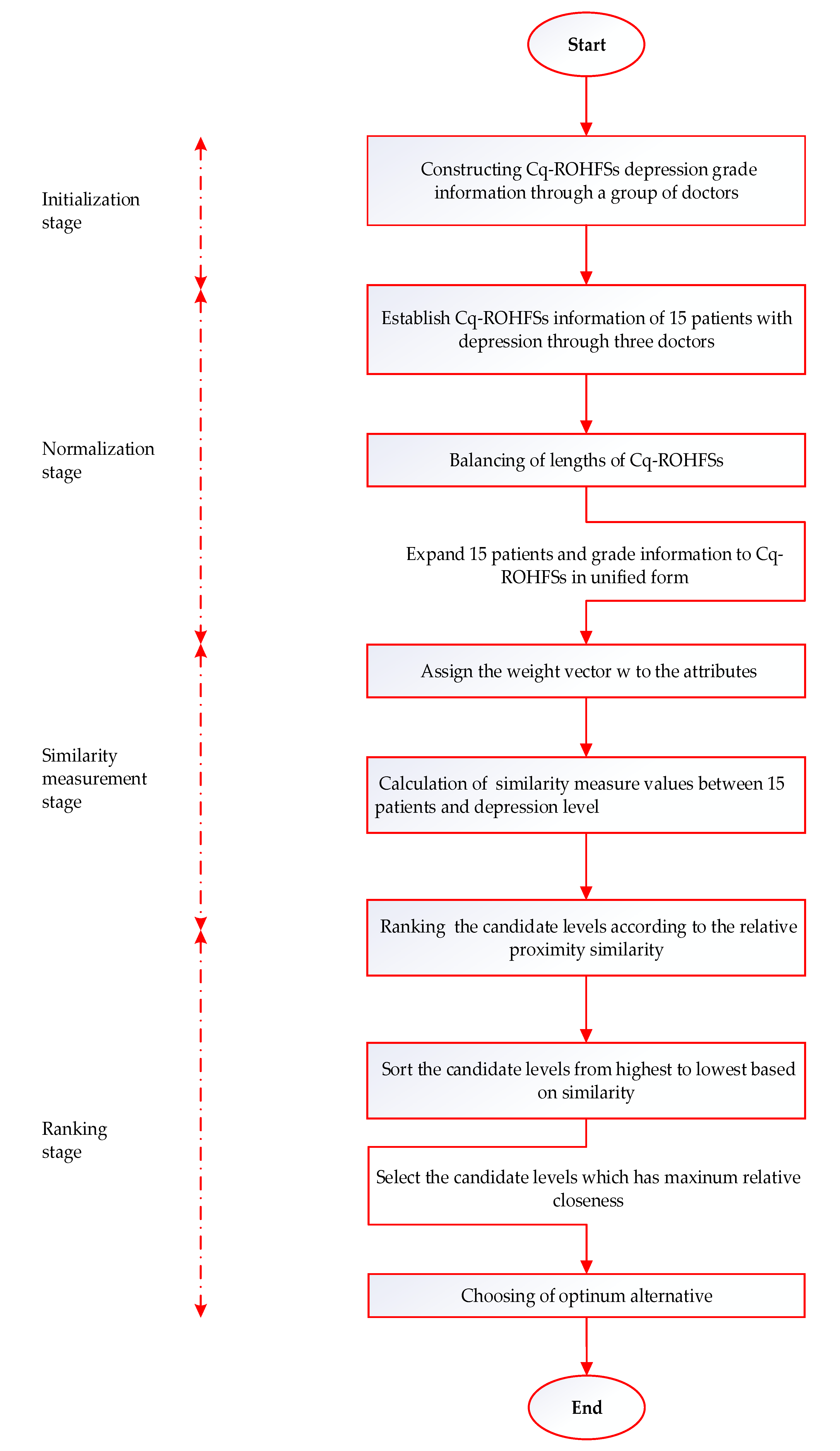
The purpose of this section is to provide 15 clinical cases as examples of how grade assessment is conducted for patients with depression to illustrate the efficacy and adaptability of the proposed depression assessment method based on Cq-ROHFS. It is recommended that the three doctors provide their evaluations anonymously in order to achieve better results. As a result, each value provided only represents a possible value, whose importance is unknown. Due to this, it is appropriate to repeat these values, rather than them appearing only once. The depression assessment method presented in this paper is depicted in Figure 2.

5.1. Numerical Illustration (15 Clinical Cases)

As shown in Table 1, we can obtain the scores of HAMD and PHQ-9 of 15 patients with depression as actual clinical cases, including the ranges of uncertain scores and membership and non-membership degrees, assigned by a group of three doctors in skeptical and hesitant situations, as indicated in

Table 3. Arguments made by 15 patients with depression (HAMD).

Patient Pi	HAMD Score	Membership of HAMD	Non-Membership of HAMD
P1	[18,21]	{0.6,0.75}	{0.25,0.35}
P2	[8,14]	{0.6,0.8}	{0.4,0.5}
P3	[20,22]	{0.3,0.65,0.85}	{0.4,0.5}
P4	[22,24]	{0.6,0.7,0.87}	{0.21,0.4}
P5	[15,18]	{0.5}	{0.5,0.6}
P6	[8,14]	{0.35}	{0.7,0.8}
P7	[21,24]	{0.4}	{0.5,0.6}
P8	[41,46]	{0.65,0.68,0.8}	{0.32,0.44}
P9	[22,25]	{0.64,0.79}	{0.35,0.65,0.68}
P10	[28,37]	{0.37,0.79}	{0.23,0.29}
P11	[46,48]	{0.59,0.75}	{0.2,0.51}
P12	[15,16]	{0.56,0.77}	{0.25,0.35}
P13	[30,34]	{0.54,0.81}	{0.23,0.39}
P14	[18,19]	{0.53,0.68}	{0.5,0.6,0.65}
P15	[40,42]	{0.61,0.82}	{0.25,0.35}

and

Table 4. Arguments made by 15 patients with depression (PHQ-9).

Patient Pi	PHQ-9 Score	Membership of PHQ-9	Non-Membership of PHQ-9
P1	[15,17]	{0.66,0.71}	{0.22,0.36}
P2	[5,6]	{0.3,0.55}	{0.35,0.55,0.81}
P3	[12,16]	{0.5,0.8}	{0.27,0.31}
P4	[18,21]	{0.8,0.88}	{0.2,0.35}
P5	[10,14]	{0.34,0.75}	{0.27,0.63}
P6	[6,7]	{0.41,0.62}	{0.57,0.61,0.87}
P7	[8,11]	{0.46,0.61}	{0.45,0.52,0.9}
P8	[18,20]	{0.55,0.83}	{0.29,0.33}
P9	[21,22]	{0.61,0.76}	{0.22,0.27}
P10	[23,24]	{0.61,0.76}	{0.27,0.34}
P11	[18,21]	{0.56,0.76}	{0.35,0.65,0.68}
P12	[5,6]	{0.3,0.55}	{0.28,0.46}
P13	[21,23]	{0.51,0.7}	{0.22,0.29,0.6}
P14	[5,9]	{0.41,0.73}	{0.23,0.51}
P15	[24,25]	{0.45,0.85}	{0.22,0.65}

.

The grade evaluation parameters of 15 patients in Table 3 and Table 4 can be transformed into standardized Cq-ROHFS, as shown in

Table 5. The Cq-ROHFS information of 15 patients with depression.

Patient Pi	C1: HAMD	C2: PHQ-9
P1	<[0.35,0.4],[0.6,0.65],{0.6,0.75},{0.25,0.35}>	<[0.56,0.63],[0.37,0.44],{0.66,0.71},{0.22,0.36}>
P2	<[0.15,0.27],[0.73,0.85],{0.6,0.8},{0.4,0.5}>	<[0.19,0.22],[0.78,0.81],{0.3,0.55},{0.35,0.55,0.81}>
P3	<[0.38,0.42],[0.58,0.62],{0.3,0.65,0.85},{0.4,0.5}>	<[0.44,0.59],[0.41,0.56],{0.5,0.8},{0.27,0.31}>
P4	<[0.42,0.46],[0.54,0.58],{0.6,0.7,0.87},{0.21,0.4}>	<[0.67,0.78],[0.22,0.33],{0.8,0.88},{0.2,0.35}>
P5	<[0.29,0.35],[0.65,0.71],{0.5},{0.5,0.6}>	<[0.37,0.52],[0.48,0.63],{0.34,0.75},{0.27,0.63}>
P6	<[0.15,0.27],[0.73,0.85],{0.35},{0.7,0.8}>	<[0.22,0.26],[0.74,0.78],{0.41,0.62},{0.57,0.61,0.87}>
P7	<[0.4,0.46],[0.54,0.6],{0.4},{0.5,0.6}>	<[0.3,0.41],[0.59,0.7],{0.46,0.61},{0.45,0.52,0.9}>
P8	<[0.79,0.88],[0.12,0.21],{0.65,0.68,0.8},{0.32,0.44}>	<[0.67,0.74],[0.26,0.33],{0.55,0.83},{0.29,0.33}>
P9	<[0.42,0.48],[0.52,0.58],{0.64,0.79},{0.35,0.65,0.68}>	<[0.78,0.81],[0.19,0.22],{0.61,0.76},{0.22,0.27}>
P10	<[0.54,0.71],[0.29,0.46],{0.37,0.79},{0.23,0.29}>	<[0.85,0.89],[0.11,0.15],{0.61,0.76},{0.27,0.34}>
P11	<[0.88,0.92],[0.08,0.12],{0.59,0.75},{0.2,0.51}>	<[0.67,0.78],[0.22,0.33],{0.56,0.76},{0.35,0.65,0.68}>
P12	<[0.29,0.31],[0.69,0.71],{0.56,0.77},{0.25,0.35}>	<[0.19,0.22],[0.78,0.81],{0.3,0.55},{0.28,0.46}>
P13	<[0.77,0.81],[0.19,0.23],{0.54,0.81},{0.23,0.39}>	<[0.78,0.85],[0.15,0.22],{0.51,0.7},{0.22,0.29,0.6}>
P14	<[0.35,0.37],[0.63,0.65],{0.53,0.68},{0.5,0.6,0.65}>	<[0.19,0.34],[0.66,0.81],{0.41,0.73},{0.23,0.51}>
P15	<[0.77,0.81],[0.19,0.23],{0.61,0.82},{0.25,0.35}>	<[0.89,0.93],[0.07,0.11],{0.45,0.85},{0.22,0.65}>

.

Then, the grade evaluation information of 15 patients with depression in Table 5 can be expressed as the following Cq-ROHFS.

$$\begin{array}{c}{P}_1=\left\{\begin{array}{l}<C_1,\left\{\left[0.35,0.4\right]\right\},\left\{\left[0.6,0.65\right]\right\},\{0.6,0.75\},\{0.25,0.35\}>,\\ <C_2,\left\{[0.56,0.63]\right\},\left\{[0.37,0.44]\right\},\{0.66,0.71\},\{0.22,0.36\}>\end{array}\right\}\hfill \\ P_2=\left\{\begin{array}{l}<C_1,\left\{[0.15,0.27]\right\},\left\{[0.73,0.85]\right\},\{0.6,0.8\},\{0.4,0.5\}>,\\ <C_2,\left\{[0.19,0.22]\right\},\left\{[0.78,0.81]\right\},\{0.3,0.55\},\{0.35,0.55,0.81\}>\end{array}\right\}\hfill \\ P_3=\left\{\begin{array}{l}<C_1,\left\{[0.38,0.42]\right\},\left\{[0.58,0.62]\right\},\{0.3,0.65,0.85\},\{0.4,0.5\}>,\\ <C_2,\left\{[0.44,0.59]\right\},\left\{[0.41,0.56]\right\},\{0.5,0.8\},\{0.27,0.31\}>\end{array}\right\}\hfill \\ P_4=\left\{\begin{array}{l}<C_1,\left\{[0.42,0.46]\right\},\left\{[0.54,0.58]\right\},\{0.6,0.7,0.87\},\{0.21,0.4\}>,\\ <C_2,\left\{[0.67,0.78]\right\},\left\{[0.22,0.33]\right\},\{0.8,0.88\},\{0.2,0.35\}>\end{array}\right\}\hfill \\ P_5=\left\{\begin{array}{l}<C_1,\left\{[0.29,0.35]\right\},\left\{[0.65,0.71]\right\},\left\{0.5\right\},\{0.5,0.6\}>,\\ <C_2,\left\{[0.37,0.52]\right\},\left\{[0.48,0.63]\right\},\{0.34,0.75\},\{0.27,0.63\}>\end{array}\right\}\hfill \\ P_6=\left\{\begin{array}{l}<C_1,\left\{[0.15,0.27]\right\},\left\{[0.73,0.85]\right\},\left\{0.35\right\},\{0.7,0.8\}>,\\ <C_2,\left\{[0.22,0.26]\right\},\left\{[0.74,0.78]\right\},\{0.41,0.62\},\{0.57,0.61,0.87\}>\end{array}\right\}\hfill \\ P_7=\left\{\begin{array}{l}<C_1,\left\{[0.4,0.46]\right\},\left\{[0.54,0.6]\right\},\left\{0.4\right\},\{0.5,0.6\}>,\\ <C_2,\left\{[0.3,0.41]\right\},\left\{[0.59,0.7]\right\},\{0.46,0.61\},\{0.45,0.52,0.9\}>\end{array}\right\}\hfill \\ P_8=\left\{\begin{array}{l}<C_1,\left\{[0.79,0.88]\right\},\left\{[0.12,0.21\right\}],\{0.65,0.68,0.8\},\{0.32,0.44\}>,\\ <C_2,\left\{[0.67,0.74]\right\},\left\{[0.26,0.33]\right\},\{0.55,0.83\},\{0.29,0.33\}>\end{array}\right\}\hfill \\ P_9=\left\{\begin{array}{l}<C_1,\left\{[0.42,0.48]\right\},\left\{[0.52,0.58]\right\},\{0.64,0.79\},\{0.35,0.65,0.68\}>,\\ <C_2,\left\{[0.78,0.81]\right\},\left\{[0.19,0.22]\right\},\{0.61,0.76\},\{0.22,0.27\}>\end{array}\right\}\hfill \\ P_{10}=\left\{\begin{array}{l}<C_1,\left\{[0.54,0.71]\right\},\left\{[0.29,0.46]\right\},\{0.37,0.79\},\{0.23,0.29\}>,\\ <C_2,\left\{[0.85,0.89]\right\},\left\{[0.11,0.15]\right\},\{0.61,0.76\},\{0.27,0.34\}>\end{array}\right\}\hfill \\ P_{11}=\left\{\begin{array}{l}<C_1,\left\{[0.88,0.92]\right\},\left\{[0.08,0.12]\right\},\{0.59,0.75\},\{0.2,0.51\}>,\\ <C_2,\left\{[0.67,0.78]\right\},\left\{[0.22,0.33]\right\},\{0.56,0.76\},\{0.35,0.65,0.68\}>\end{array}\right\}\hfill \\ P_{12}=\left\{\begin{array}{l}<C_1,\left\{[0.29,0.31]\right\},\left\{[0.69,0.71]\right\},\{0.56,0.77\},\{0.25,0.35\}>,\\ <C_2,\left\{[0.19,0.22]\right\},\left\{[0.78,0.81]\right\},\{0.3,0.55\},\{0.28,0.46\}>\end{array}\right\}\hfill \\ P_{13}=\left\{\begin{array}{l}<C_1,\left\{[0.77,0.81]\right\},\left\{[0.19,0.23]\right\},\{0.54,0.81\},\{0.23,0.39\}>,\\ <C_2,\left\{[0.78,0.85]\right\},\left\{[0.15,0.22]\right\},\{0.51,0.7\},\{0.22,0.29,0.6\}>\end{array}\right\}\hfill \\ P_{14}=\left\{\begin{array}{l}<C_1,\left\{[0.35,0.37]\right\},\left\{[0.63,0.65]\right\},\{0.53,0.68\},\{0.5,0.6,0.65\}>,\\ <C_2,\left\{[0.19,0.34]\right\},\left\{[0.66,0.81]\right\},\{0.41,0.73\},\{0.23,0.51\}>\end{array}\right\}\hfill \\ P_{15}=\left\{\begin{array}{l}<C_1,\left\{[0.77,0.81]\right\},\left\{[0.19,0.23]\right\},\{0.61,0.82\},\{0.25,0.35\}>,\\ <C_2,\left\{[0.89,0.93]\right\},\left\{[0.07,0.11]\right\},\{0.45,0.85\},\{0.22,0.65\}>\end{array}\right\}\hfill \end{array}$$

Based upon the assumption that the weight of each element $C_s$ is the same, $s=1,2$ and $w_s=1/2$. Using Equations (22) and (23), we can calculate the similarity measure between patient $P_i$$(i=1,2,\dots ,15)$ and depression grade $D_k(k=1,2,3)$.

5.2. Result and Discussion

At present, no other method can be used to more accurately determine depression ratings. In this section, we compare the proposed depression rating assessment model with the existing commonly utilized HAMD and PHQ-9 assessment methods [50,51,52] using 15 depressed patients. Our proposed structure is also evaluated for its superiority, validity, veracity, and symmetry. Based on our observations, we observe that our proposed model is superior and can successfully handle the DM decision problem.

In the first step, we used Equation (13) to adjust only the parameter $q$ in order to produce a more accurate representation of the patient assessment information in the decision-making process. To investigate the effect of different values of $q=1,2,3,\dots ,10$ on the grade assessment results, the analytical calculations were chosen, and the above steps were repeated in order to obtain the similarity results of patient $P_i$$(i=1,2,\dots ,15)$ and depressive symptoms $D_k(k=1,2,3)$, as shown in

Table 6. Similarity measurements between $P_i$ and $D_k$ $\left(i=1,2,3,k=1,2,3,q=1,2,3,\dots ,10\right)$.

$S_{ewg}(P_i,D_k)$	Patient Pi
	$P_1$	$P_2$	$P_3$
$q=1$	0.8509, 0.9288, 0.8349	0.8974, 0.8208, 0.7074	0.8598, 0.9202, 0.8091
$q=2$	0.7778, 0.8841, 0.7209	0.8415, 0.7595, 0.5800	0.8013, 0.8716, 0.7094
$q=3$	0.7312, 0.8572, 0.6363	0.8003, 0.7164, 0.4947	0.7683, 0.8378, 0.6417
$q=4$	0.6985, 0.8385, 0.5758	0.7711, 0.6847, 0.4355	0.7469, 0.8142, 0.5923
$q=5$	0.6740, 0.8246, 0.5319	0.7496, 0.6596, 0.3926	0.7318, 0.7972, 0.5545
$q=6$	0.6550, 0.8136, 0.4989	0.7332, 0.6393, 0.3604	0.7206, 0.7844, 0.5249
$q=7$	0.6399, 0.8046, 0.4734	0.7204, 0.6224, 0.3355	0.7119, 0.7744, 0.5009
$q=8$	0.6276, 0.7973, 0.4532	0.7101, 0.6082, 0.3159	0.7049, 0.7664, 0.4814
$q=9$	0.6173, 0.7910, 0.4367	0.7017, 0.5962, 0.3000	0.7008, 0.7610, 0.4679
$q=10$	0.6087, 0.7858, 0.4231	0.6947, 0.5859, 0.2869	0.6945, 0.7542, 0.4513
$S_{ewg}(P_i,D_k)$	Patient Pi
	$P_4$	$P_5$	$P_6$
$q=1$	0.7971, 0.8863, 0.8858	0.8616,0.8764,0.7330	0.8114,0.7377,0.6276
$q=2$	0.7081, 0.8261, 0.7865	0.7864, 0.7917, 0.6281	0.7197, 0.6642, 0.5293
$q=3$	0.6482, 0.7860, 0.7066	0.7291, 0.7258, 0.5614	0.6610, 0.6180, 0.4689
$q=4$	0.6062, 0.7569, 0.6453	0.6812, 0.6744, 0.5140	0.6207, 0.5846, 0.4252
$q=5$	0.5758, 0.7348, 0.5990	0.6414, 0.6345, 0.4784	0.5911, 0.5590, 0.3915
$q=6$	0.5531, 0.7174, 0.5639	0.6088, 0.6034, 0.4508	0.5683, 0.5387, 0.3649
$q=7$	0.5355, 0.7036, 0.5368	0.5826, 0.5785, 0.4319	0.5501, 0.5222, 0.3435
$q=8$	0.5215, 0.6923, 0.5153	0.5611, 0.5583, 0.4105	0.5351, 0.5086, 0.3261
$q=9$	0.5128, 0.6847, 0.5007	0.5436, 0.5416, 0.3955	0.5226, 0.4971, 0.3117
$q=10$	0.5008, 0.6752, 0.4837	0.5290, 0.5276, 0.3828	0.5120, 0.4873, 0.2997
$S_{ewg}(P_i,D_k)$	Patient Pi
	$P_7$	$P_8$	$P_9$
$q=1$	0.8115, 0.8216, 0.7098	0.7676, 0.8400, 0.8931	0.7821, 0.8464, 0.8432
$q=2$	0.7367, 0.7323, 0.6150	0.6418, 0.7527, 0.8278	0.6754, 0.771, 0.7576
$q=3$	0.6843, 0.6721, 0.5577	0.5659, 0.6939, 0.7843	0.6036, 0.7164, 0.6913
$q=4$	0.6448, 0.6286, 0.5190	0.5157, 0.6523, 0.7536	0.5535, 0.6756, 0.6393
$q=5$	0.6139, 0.5961, 0.4910	0.4798, 0.6218, 0.7309	0.5172, 0.6447, 0.5993
$q=6$	0.5889, 0.5710, 0.4697	0.4525, 0.5988, 0.7134	0.4899, 0.621, 0.5684
$q=7$	0.5683, 0.5511, 0.4530	0.4309, 0.5808, 0.6997	0.4685, 0.6026, 0.5443
$q=8$	0.5511, 0.5351, 0.4394	0.4131, 0.5665, 0.6885	0.4513, 0.5879, 0.525
$q=9$	0.5365, 0.5219, 0.4282	0.4015, 0.5572, 0.6809	0.4402, 0.5783, 0.512
$q=10$	0.5240, 0.5108, 0.4187	0.3856, 0.5451, 0.6714	0.4254, 0.5662, 0.4963
$S_{ewg}(P_i,D_k)$	Patient Pi
	$P_{10}$	$P_{11}$	$P_{12}$
$q=1$	0.7541, 0.8344, 0.8847	0.7469, 0.8165, 0.8848	0.9207, 0.8656, 0.7308
$q=2$	0.6237, 0.7482, 0.8244	0.5987, 0.6962, 0.7803	0.8641, 0.7845, 0.5793
$q=3$	0.5479, 0.6899, 0.7854	0.5123, 0.6286, 0.7242	0.828, 0.7285, 0.4878
$q=4$	0.4981, 0.6456, 0.7574	0.4558, 0.5824, 0.6831	0.8027, 0.6876, 0.428
$q=5$	0.4624, 0.6109, 0.7364	0.4157, 0.5494, 0.6524	0.7836, 0.6569, 0.3861
$q=6$	0.4354, 0.5835, 0.72	0.3854, 0.5249, 0.629	0.7685, 0.6331, 0.3551
$q=7$	0.4141, 0.5617, 0.707	0.3615, 0.5058, 0.6109	0.7561, 0.6143, 0.3312
$q=8$	0.3969, 0.5441, 0.6965	0.3421, 0.4906, 0.5964	0.7458, 0.5992, 0.3124
$q=9$	0.3826, 0.5297, 0.6879	0.326, 0.4782, 0.5848	0.737, 0.5868, 0.297
$q=10$	0.3707, 0.5178, 0.6807	0.3125, 0.4678, 0.5751	0.7295, 0.5764, 0.2843
$S_{ewg}(P_i,D_k)$	Patient Pi
	$P_{13}$	$P_{14}$	$P_{15}$
$q=1$	0.7920, 0.8619, 0.8785	0.9077, 0.8595, 0.7375	0.7219, 0.8023, 0.8816
$q=2$	0.6741, 0.7923, 0.8194	0.8464, 0.7958, 0.6182	0.5723, 0.6948, 0.8211
$q=3$	0.6013, 0.7439, 0.7732	0.8025, 0.7568, 0.5416	0.4903, 0.6313, 0.7833
$q=4$	0.5531, 0.7064, 0.7362	0.7695, 0.7289, 0.4894	0.4403, 0.5895, 0.7574
$q=5$	0.5188, 0.6761, 0.7071	0.7439, 0.7073, 0.4521	0.4066, 0.5593, 0.7382
$q=6$	0.493, 0.6514, 0.6843	0.7232, 0.6899, 0.4243	0.3823, 0.5363, 0.7231
$q=7$	0.4729, 0.6311, 0.6664	0.7061, 0.6755, 0.4029	0.3637, 0.518, 0.7109
$q=8$	0.4566, 0.6144, 0.6521	0.6917, 0.6633, 0.3858	0.349, 0.5031, 0.7008
$q=9$	0.4431, 0.6005, 0.6405	0.681, 0.6547, 0.3753	0.337, 0.4905, 0.6922
$q=10$	0.4317, 0.5889, 0.6309	0.6687, 0.6438, 0.3605	0.327, 0.4799, 0.6849

.

Depending on the physician’s experience, testing time, and judgment, the data gathered from patients who are depressed may contain a certain amount of uncertainty and ambiguity. In these instances, existing methods of diagnosing depression [50,51,52] rely primarily on precise numerical measurements to describe and rate the grade of depression. As a consequence, the depression data of some patients may belong to different depression grades, thus producing inaccurate or inconclusive assessment results and complicating the assessment process.

In order to demonstrate the validity of the proposed method, we used only the mean of the interval membership set of Cq-ROHFS, thus simplifying Cq-ROHFS to the exact value. For example, for the interval membership of $P_1$, the average of 0.35 and 0.4 is 0.375, and the average of 0.56 and 0.63 is 0.595. The results are shown in

Table 7. The exact values of the 15 patients.

Patient Pi	${\mathit{C}}_1:\mathbf{HAMD}$	${\mathit{C}}_2:\mathbf{PHQ}-9$
$P_1$	0.375	0.595
$P_2$	0.22	0.205
$P_3$	0.4	0.515
$P_4$	0.44	0.725
$P_5$	0.32	0.445
$P_6$	0.22	0.24
$P_7$	0.43	0.355
$P_8$	0.835	0.705
$P_9$	0.45	0.795
$P_{10}$	0.625	0.87
$P_{11}$	0.9	0.725
$P_{12}$	0.3	0.205
$P_{13}$	0.79	0.805
$P_{14}$	0.36	0.265
$P_{15}$	0.79	0.91

.

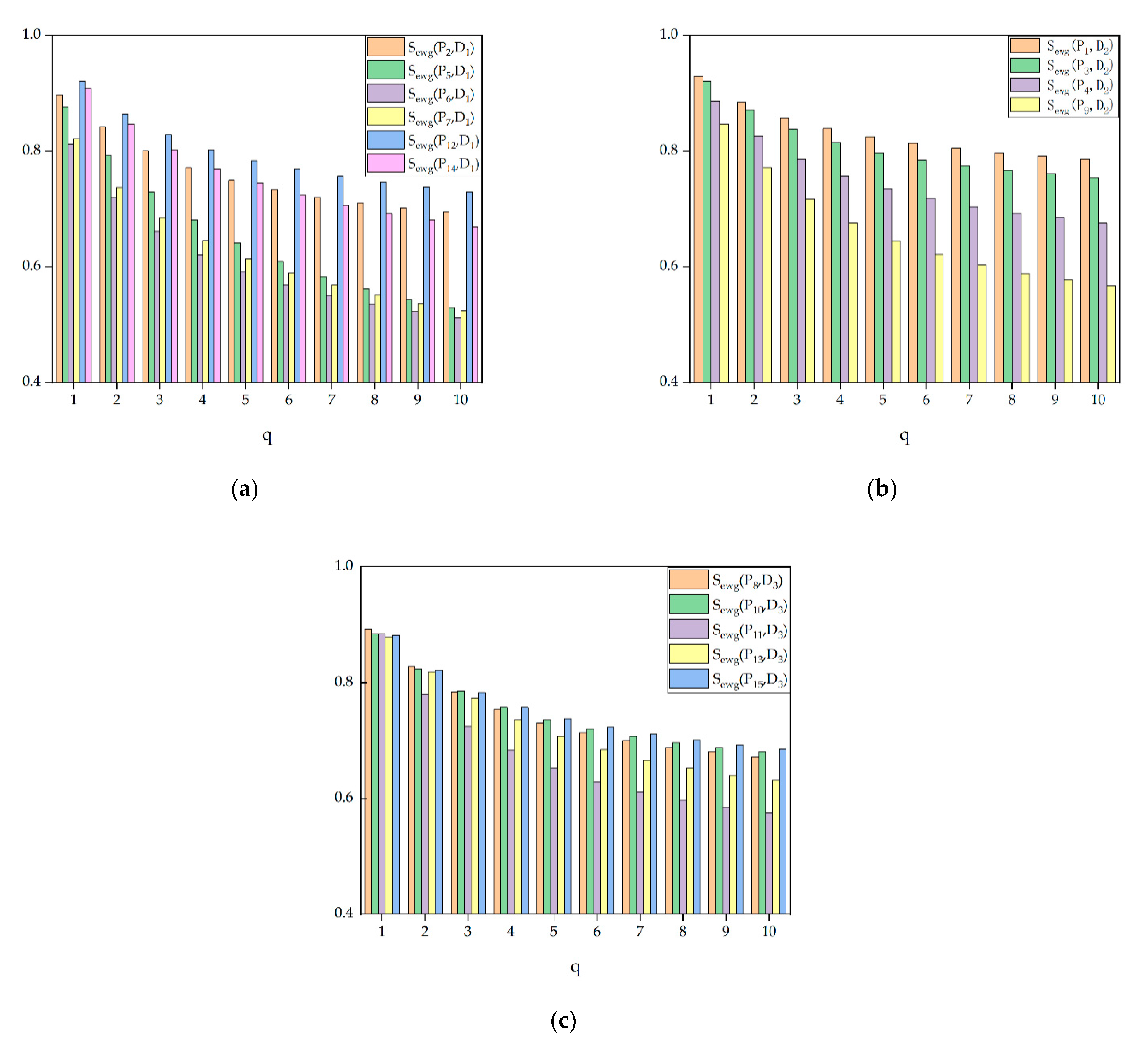
Then, we examined the effect of parameters on the results of depression grade diagnosis. Based on Table 6, the parameters have an effect on the similarity results, and the degree of similarity gradually increases as parameter $q$ is increased. However, the final similarity results of depression grades remained unchanged. The depression grade in Table 6 is determined by the maximum similarity. As an example, for $P_2$, the greatest similarity is with $D_1$, so $P_2$ belongs to $D_1$, i.e., Mild Depression. Therefore, this study’s method of evaluating depression allows the development of a composite depression scale based on 15 clinical cases, shown in

Table 8. Comparison of the evaluated depression levels of 15 patients $P_i$.

Patient Pi	Depression Grade of the Proposed Evaluation Method Use ${\mathit{S}}_{\mathit{e}\mathit{w}\mathit{g}}({\mathit{P}}_{\mathit{i}},{\mathit{D}}_{\mathit{k}})$	Grade of Depression According to Tang and Zhang [50]	Grade of Depression According to Kurt et al. [51]	Grade of Depression According to Guo et al. [52]
$P_1$	$D_2$	$D_2$	$D_2$	$D_2$
$P_2$	$D_1$	$D_1$	$D_1$	$D_1$
$P_3$	$D_2$	$D_2$	$D_2$	$D_2$
$P_4$	$D_2$	$D_2$	$D_3$	$D_2$ or $D_3$
$P_5$	$D_1$	$D_1$	$D_2$	$D_1$ or $D_2$
$P_6$	$D_1$	$D_1$	$D_1$	$D_1$
$P_7$	$D_1$	$D_1$	$D_1$ or $D_2$	$D_1$ or $D_2$
$P_8$	$D_3$	$D_3$	$D_3$	$D_3$
$P_9$	$D_2$	$D_2$	$D_3$	$D_2$ or $D_3$
$P_{10}$	$D_3$	$D_3$	$D_3$	$D_3$
$P_{11}$	$D_3$	$D_3$	$D_3$	$D_3$
$P_{12}$	$D_1$	$D_1$	$D_1$	$D_1$
$P_{13}$	$D_3$	$D_3$	$D_3$	$D_3$
$P_{14}$	$D_1$	$D_2$	$D_1$	$D_1$ or $D_2$
$P_{15}$	$D_3$	$D_3$	$D_3$	$D_3$

, which is then compared with the previously available methods of depression measurement.

Hence, depression grades can be calculated using the method proposed by [50,51,52] in correlation with Table 1 and Table 7, and the results are also presented in Table 8. In this case, the existing methods cannot accurately assess or diagnose the degree of depression for five patients $P_4$, $P_5$, $P_7$, $P_9$, and $P_{14}$. It is evident from Table 8 that the diagnostic results of 15 depressed patients who used the existing assessment method were comparable to or consistent with those of the newly proposed method. Consequently, the proposed evaluation method is an exponential similarity measure of Cq-ROHFSs based on Equation (13), which overcomes the drawbacks of existing simple scoring evaluation methods that have uncertain results. The proposed approach can provide accurate and unique assessment results, proving its validity and rationality.

In Table 8, according to the method described in this article, patients $P_2,P_5,P_6,P_7,P_{12}$ and $P_{14}$ were mildly depressed, $P_1,P_3,P_4$ and $P_9$ were moderately depressed, and $P_8,P_{10},P_{11},P_{13}$ and $P_{15}$ were severely depressed. As shown in Figure 3, the degree of difference in similarity gradually increased as $q$ increased.

As part of this section, we extend the exponential distance based on Cq-ROHFS to an exponential distance with hesitancy. Using Equation (14), we can then estimate the similarity between the 15 patients and the degree of hesitation, the degree of membership, and the degree of non-membership. The preference is different with diverse values of $\alpha$, $\beta$, $\gamma$, $\eta$ and $\alpha ,\beta ,\lambda ,\eta \in \left[0,1\right]$, $\alpha +\beta =1,\lambda +\eta =1$. Take $q=2$, $\alpha =\gamma$ and $\alpha =0.1,0.2,0.5,0.6,0.8,0.9$ respectively; we use the formula to compute the similarity between the 15 depressed patients and their depressive symptoms, as shown in

Table 9. The similarity result with preference ($q=2$).

$S_{ewpg}(P_i,D_k)$	Patient Pi
	$P_1$	$P_2$	$P_3$
$\alpha =0.1$	0.8286, 0.9015, 0.7911	0.8556, 0.8006, 0.6722	0.8436, 0.8851, 0.7717
$\alpha =0.2$	0.831, 0.9051, 0.7923	0.8624, 0.8063, 0.6758	0.8466, 0.8903, 0.7754
$\alpha =0.5$	0.8387, 0.9169, 0.7959	0.8858, 0.825, 0.6868	0.8562, 0.9079, 0.7872
$\alpha =0.6$	0.8413, 0.9213, 0.7972	0.895, 0.8318, 0.6906	0.8596, 0.9146, 0.7913
$\alpha =0.8$	0.8468, 0.931, 0.7997	0.9167, 0.8465, 0.6985	0.8666, 0.9303, 0.7998
$\alpha =0.9$	0.8496, 0.9364, 0.8009	0.9304, 0.8545, 0.7025	0.8703, 0.9399, 0.8043
$S_{ewpg}(P_i,D_k)$	Patient Pi
	$P_4$	$P_5$	$P_6$
$\alpha =0.1$	0.7743, 0.8602, 0.8395	0.8516, 0.8459, 0.719	0.7604, 0.7151, 0.6176
$\alpha =0.2$	0.7772, 0.8636, 0.8409	0.8499, 0.8467, 0.7204	0.7684, 0.7238, 0.6245
$\alpha =0.5$	0.7862, 0.8745, 0.8452	0.8451, 0.8491, 0.7246	0.795, 0.7526, 0.6464
$\alpha =0.6$	0.7893, 0.8784, 0.8467	0.8436, 0.8499, 0.726	0.8049, 0.7632, 0.6542
$\alpha =0.8$	0.7957, 0.8865, 0.8497	0.8405, 0.8515, 0.7289	0.827, 0.7867, 0.6706
$\alpha =0.9$	0.799, 0.8909, 0.8512	0.839, 0.8523, 0.7304	0.8394, 0.7998, 0.6793
$S_{ewpg}(P_i,D_k)$	Patient Pi
	$P_7$	$P_8$	$P_9$
$\alpha =0.1$	0.7913, 0.7783, 0.6924	0.7301, 0.8134, 0.8691	0.7486, 0.8117, 0.8018
$\alpha =0.2$	0.7953, 0.7845, 0.6977	0.7314, 0.815, 0.8707	0.751, 0.8173, 0.8067
$\alpha =0.5$	0.8078, 0.8045, 0.7144	0.7352, 0.8199, 0.8758	0.7612, 0.8336, 0.8236
$\alpha =0.6$	0.8122, 0.8118, 0.7202	0.7365, 0.8216, 0.8775	0.7645, 0.8397, 0.8296
$\alpha =0.8$	0.8215, 0.8275, 0.7325	0.7392, 0.8251, 0.8811	0.7713, 0.8527, 0.8424
$\alpha =0.9$	0.8264, 0.8361, 0.739	0.7405, 0.8268, 0.883	0.7748, 0.8598, 0.8493
$S_{ewpg}(P_i,D_k)$	Patient Pi
	$P_{10}$	$P_{11}$	$P_{12}$
$\alpha =0.1$	0.7157, 0.809, 0.8576	0.6961, 0.7667, 0.822	0.8799, 0.8279, 0.6776
$\alpha =0.2$	0.7171, 0.8109, 0.8613	0.6974, 0.7693, 0.8264	0.8851, 0.8317, 0.6798
$\alpha =0.5$	0.7211, 0.8165, 0.8733	0.7016, 0.7771, 0.8405	0.9024, 0.8437, 0.6863
$\alpha =0.6$	0.7225, 0.8185, 0.8776	0.703, 0.7798, 0.8456	0.909, 0.848, 0.6885
$\alpha =0.8$	0.7253, 0.8224, 0.8867	0.7059, 0.7853, 0.8564	0.9241, 0.8569, 0.693
$\alpha =0.9$	0.7267, 0.8244, 0.8917	0.7074, 0.7882, 0.8622	0.9331, 0.8617, 0.6953
	$P_{13}$	$P_{14}$	$P_{15}$
$\alpha =0.1$	0.7563, 0.844, 0.8609	0.8655, 0.827, 0.7018	0.6779, 0.7724, 0.8623
$\alpha =0.2$	0.7573, 0.8453, 0.863	0.8708, 0.8328, 0.7061	0.6786, 0.7733, 0.8643
$\alpha =0.5$	0.7602, 0.8495, 0.8696	0.8894, 0.8521, 0.7169	0.6808, 0.776, 0.8708
$\alpha =0.6$	0.7611, 0.8509, 0.8718	0.8964, 0.8592, 0.7209	0.6815, 0.7769, 0.873
$\alpha =0.8$	0.7631, 0.8538, 0.8765	0.9122, 0.8748, 0.729	0.683, 0.7788, 0.8777
$\alpha =0.9$	0.7641, 0.8553, 0.8789	0.9215, 0.8836, 0.7332	0.6837, 0.7797, 0.8801

.

According to Table 9, as $\alpha$ changes, similarity results also change, which means that the degree of hesitation influences the final decision. In particular, when $\alpha$ increases, for example $\alpha =0.6$, we tend to focus more on the differences between hesitations rather than the differences between values. This is because the differences between hesitations have a stronger effect than the differences between values, and this effect is sufficient to compensate for the differences between values. Thus, as $\alpha$ changes, the depression levels in

Table 10. Grading depression with preference ($q=2$ ).

Depression Grade	$\alpha =0.1$	$\alpha =0.2$	$\alpha =0.5$	$\alpha =0.6$	$\alpha =0.8$	$\alpha =0.9$
$P_1$	$D_2$	$D_2$	$D_2$	$D_2$	$D_2$	$D_2$
$P_2$	$D_1$	$D_1$	$D_1$	$D_1$	$D_1$	$D_1$
$P_3$	$D_2$	$D_2$	$D_2$	$D_2$	$D_2$	$D_2$
$P_4$	$D_2$	$D_2$	$D_2$	$D_2$	$D_2$	$D_2$
$P_5$	$D_1$	$D_2$	$D_2$	$D_2$	$D_2$	$D_2$
$P_6$	$D_1$	$D_1$	$D_1$	$D_1$	$D_1$	$D_1$
$P_7$	$D_1$	$D_1$	$D_1$	$D_1$	$D_2$	$D_2$
$P_8$	$D_3$	$D_3$	$D_3$	$D_3$	$D_3$	$D_3$
$P_9$	$D_2$	$D_2$	$D_2$	$D_2$	$D_2$	$D_2$
$P_{10}$	$D_3$	$D_3$	$D_3$	$D_3$	$D_3$	$D_3$
$P_{11}$	$D_3$	$D_3$	$D_3$	$D_3$	$D_3$	$D_3$
$P_{12}$	$D_1$	$D_1$	$D_1$	$D_1$	$D_1$	$D_1$
$P_{13}$	$D_3$	$D_3$	$D_3$	$D_3$	$D_3$	$D_3$
$P_{14}$	$D_1$	$D_1$	$D_1$	$D_1$	$D_1$	$D_1$
$P_{15}$	$D_3$	$D_3$	$D_3$	$D_3$	$D_3$	$D_3$

changes accordingly. This is due to the fact that the hesitation fuzzy set focuses on describing situations in which individuals are hesitant to provide preferences during the decision-making process. Therefore, it is reasonable to expect the level of hesitation to affect the decision outcome. $S_{ewg}(P_i,D_k)$ and $S_{ewpg}(P_i,D_k)$ $(q=2)$ differ in their results because of different preferences for the parameters $\alpha ,\beta ,\gamma ,\eta$. Therefore, the decision maker is able to make an informed decision based on the facts and circumstances at hand.

5.3. Comparison Analysis

Consequently, the evaluation results of the proposed comprehensive evaluation method for depression are included in or equal to those of the evaluation. This is sufficient to demonstrate the validity of the methodology. Due to the existing method, some depressed patients may receive inaccurate or unclear grade evaluations, resulting in a complicated assessment. As a consequence, the depression evaluation data from the two existing criteria may involve patients with varying degrees of depression simultaneously. Additionally, it is shown that the depression rating assessment method proposed in this paper is reasonable and can clearly demonstrate the performance of 15 depressed patients.

In

Table 11. Comparison of the proposed Cq-ROHFS with existing theories.

SN	References	Disadvantage	Grade Diagnosis
1	Zedah [1]	Lack of non-membership	Not Possible
2	Mehmood et al. [43]	Lack of non-membership	Not Possible
3	Liu et al. [44]	Lack of Interval fuzzy values	Not Possible
4	Guo et al. [50]	Lack of fuzzy values	Partially undetermined
5	Tang and Zhang [51]	Lack of PHQ-9 scores	Partially undetermined
6	Kurt et al. [52]	Lack of HAMD scores	Partially undetermined
7	Proposed Method in this paper	Long and heavy calculations in grades diagnosis	This problem can be solved with the help of a computer program

, the proposed Cq-ROHFS is compared with existing theories.In contrast to the previous study, Zedah [1] and Mehmood et al. [43] considered ambiguous information, but the final results were not able to be calculated since they considered only membership and not non-membership. It is noteworthy that Liu et al. [44] failed to consider the possibility that depression information may have an uncertain interval value form. The study by Tang and Zhang [50] focused solely on the HAMD and exact number depression scale assessment methods, which had one-sided results and were inaccurate. Using only the PHQ-9, Kurt et al. [51] analyzed the depression scale, which led to an incomplete assessment of the results. Guo et al. [52] considered both depression scales and exact numbers simultaneously, but it was difficult to make a selection when the results obtained from both depression scales were attributed to different levels at the same time. According to the method proposed in this paper, uncertain and hesitant information can be dealt with in an integrated manner. This problem can be solved with the aid of a computer program, exact results can be obtained, and information about the decision maker’s preferences can be considered. The long calculation time and workload required in the diagnosis of depression levels is a defect of our method.

In this paper, the Cq-ROHFS similarity measure is presented as a useful mathematical tool for decision making. It is capable of being applied to the assessment of depression as a whole. Advanced diagnostic methods are more suitable and practical for the initial evaluation of depressive symptoms, with greater effectiveness and rationality than existing methods.

6. Conclusions

A cubic q-rung orthopair hesitant fuzzy set is a novel extension of CIHFS and CPHFS, and a generalization of both concepts. A Cq-ROHFS contains more information and can be used to calculate both IVq-ROHFS and q-ROHFS in order to deal with the fuzziness of information. The fuzzy set theory gives decision makers greater scope to express their opinions. Asymmetric concepts are particularly relevant to decision making, since they characterize the binary relationship used to model the decision maker’s preferences. Our study presents a preliminary assessment model for depression rating based on cubic q-rung orthopair hesitant fuzzy set theory from the perspective of multi-attribute decision making. We discussed some basic concepts and developed some basic operations regarding Cq-ROHFS and its properties in this study. First, we introduced the basic properties and definition of Cq-ROHFS. Then, a new concept of exponential distance and similarity measures is proposed for Cq-ROHFS with hesitation based on the LCM extension method for the Cq-ROHF set. Additionally, for decision problems, an approach is developed based on the use of similarity measures in a Cq-ROHFS setting. To test the validity, flexibility, and applicability of the developed decision model, we used the developed model to address the depression rating assessment decision problem. Clinical cases were used to compare the proposed method with existing methods. The proposed evaluation method can be used to efficiently and rationally resolve the problem of depression rating assessment. The following are some strengths of the developed method: 1. When faced with uncertain information and indecision, it is capable of expressing and dealing with decision-making problems rationally and effectively. 2. The extension-based LCM method demonstrates an objective extension operation without subjective extension forms. 3. The proposed method permits the decision maker to adjust the parameters according to their preferences during decision making, in order to express their assessment information more accurately. Moreover, the study contributes to the scientific community by illustrating real-world clinical diagnostic problems and treatments. Because Cq-ROHFS enables a flexible and convenient means of expressing information and making decisions, it is applicable to a wide range of decision-making problems. The application of Cq-ROHFS to practical and complex decision problems is a topic of research that has broad application prospects and profound social implications. A further research project will investigate whether decision problems [25,26] can be addressed in this manner. Moreover, we intend to extend the proposed study to other settings, such as linear Diophantine fuzzy sets and spherical linear Diophantine fuzzy sets. Further, we will propose some aggregation operators that contain Cq-ROHFS information, along with new systematic metrics for evaluating information.

References

- Zadeh, L.A. Fuzzy sets. Inf. Control 1965, 8, 338–353. [Google Scholar] [CrossRef] [Green Version]
- Atanassov, K. Intuitionistic fuzzy sets. Fuzzy Sets Syst. 1986, 20, 87–96. [Google Scholar] [CrossRef]
- Atanassov, K.; Gargov, G. Interval valued intuitionistic fuzzy sets. Fuzzy Sets Syst. 1989, 31, 343–349. [Google Scholar] [CrossRef]
- Yager, R.R. Pythagorean fuzzy subsets. In Proceedings of the Joint IFSA World Congress and NAFIPS Annual Meeting, Edmonton, AB, Canada, 24–28 June 2013; pp. 57–61. [Google Scholar]
- Garg, H. A novel accuracy function under interval-valued Pythagorean fuzzy environment for solving multicriteria decision making problem. J. Intell. Fuzzy Syst. 2016, 31, 529–540. [Google Scholar] [CrossRef]
- Senapati, T.; Yager, R.R. Fermatean fuzzy sets. J. Ambient. Intell. Humaniz. Comput. 2020, 11, 663–674. [Google Scholar] [CrossRef]
- Jeevaraj, S. Ordering of interval-valued Fermatean fuzzy sets and its applications. Expert Syst. Appl. 2021, 185, 115613. [Google Scholar]
- Yager, R.R. Generalized Orthopair fuzzy Sets. IEEE Trans. Fuzzy Syst. 2017, 25, 1222–1230. [Google Scholar] [CrossRef]
- Liu, P.; Wang, P. Some q-Rung Orthopair Fuzzy Aggregation Operators and their Applications to Multiple-Attribute Decision Making. Int. J. Intell. Syst. 2018, 33, 259–280. [Google Scholar] [CrossRef]
- Peng, X.; Dai, J. Research on the assessment of classroom teaching quality with q-rung orthopair fuzzy information based on multiparametric similarity measure and combinative distance-based assessment. Int. J. Intell. Syst. 2019, 34, 1588–1630. [Google Scholar] [CrossRef]
- Wang, P.; Wang, J.; Wei, G.; Wei, C. Similarity measures of q-rung orthopair fuzzy sets based on cosine function and their applications. Mathematics 2019, 7, 340. [Google Scholar] [CrossRef] [Green Version]
- Liu, D.; Huang, A. Consensus reaching process for fuzzy behavioral TOPSIS method with probabilistic linguistic q-rung orthopair fuzzy set based on correlation measure. Int. J. Intell. Syst. 2020, 35, 494–528. [Google Scholar] [CrossRef]
- Peng, X.; Krishankumar, R.; Ravichandran, K. Generalized orthopair fuzzy weighted distance-based approximation (WDBA) algorithm in emergency decision-making. Int. J. Intell. Syst. 2019, 34, 2364–2402. [Google Scholar] [CrossRef]
- Krishankumar, R.; Ravichandran, K.S.; Kar, S.; Cavallaro, F.; Zavadskas, E.K.; Mardani, A. Scientific decision framework for evaluation of renewable energy sources under q-rung orthopair fuzzy set with partially known weight information. Sustainability 2019, 11, 4202. [Google Scholar] [CrossRef] [Green Version]
- Li, Z.; Wei, G.; Wang, R.; Wu, J.; Wei, C.; Wei, Y. EDAS method for multiple attribute group decision making under q-rung orthopair fuzzy environment. Technol. Econ. Dev. Econ. 2019, 26, 86–102. [Google Scholar] [CrossRef]
- Mi, X.; Li, J.; Liao, H.; Kazimieras Zavadskas, E.; Al-Barakati, A.; Barnawi, A.; Herrera-Viedma, E. Hospitality brand management by a score-based q-rung orthopair fuzzy VIKOR method integrated with the best worst method. Econ. Res. Ekon. Istraz. 2019, 32, 3266–3295. [Google Scholar]
- Deng, X.; Cheng, X.; Gu, J.; Xu, Z. An Innovative Indicator System and Group Decision Framework for Assessing Sustainable Development Enterprises. Group Decis. Negot. 2021, 30, 1201. [Google Scholar] [CrossRef]
- Peng, X.; Huang, H. Fuzzy decision making method based on CoCoSo with CRITIC for financial risk evaluation. Technol. Econ. Dev. Econ. 2020, 26, 695–724. [Google Scholar] [CrossRef] [Green Version]
- Joshi, B.P.; Singh, A.; Bhatt, P.K.; Vaisla, K.S. Interval valued q-rung orthopair fuzzy sets and their properties. Intell. Fuzzy Syst. 2018, 35, 5225–5230. [Google Scholar] [CrossRef]
- Wang, J.; Gao, H.; Wei, G.; Wei, Y. Methods for multiple-attribute group decision making with q-rung interval-valued orthopair fuzzy information and their applications to the selection of green suppliers. Symmetry 2019, 11, 56. [Google Scholar] [CrossRef] [Green Version]
- Riaz, M.; Hashmi, M.R. Linear Diophantine fuzzy set and its applications towards multi-attribute decision-making problems. J. Intell. Fuzzy Syst. 2019, 37, 5417–5439. [Google Scholar] [CrossRef]
- Ayub, S.; Shabir, M.; Riaz, M.; Aslam, M.; Chinram, R. Linear Diophantine fuzzy relations and their algebraic properties with decision making. Symmetry 2021, 13, 945. [Google Scholar] [CrossRef]
- Riaz, M.; Hashmi, M.R.; Pamucar, D.; Chu, Y.M. Spherical linear Diophantine fuzzy sets with modeling uncertainties in MCDM. Comput. Model. Eng. Sci. 2021, 126, 1125–1164. [Google Scholar] [CrossRef]
- Kutlu Gündoğdu, F.; Kahraman, C. Spherical fuzzy sets and spherical fuzzy TOPSIS method. J. Intell. Fuzzy Syst. 2019, 36, 337–352. [Google Scholar] [CrossRef]
- Seikh, M.R.; Dutta, S.; Li, D.-F. Solution of matrix games with rough interval pay-offs and its application in the telecom market share problem. Int. J. Intell. Syst. 2021, 36, 6066–6100. [Google Scholar] [CrossRef]
- Karmakar, S.; Seikh, M.R.; Castillo, O. Type-2 intuitionistic fuzzy matrix games based on a new distance measure: Application to biogas-plant implementation problem. Appl. Soft Comput. 2021, 106, 107357. [Google Scholar] [CrossRef]
- Jun, Y.B.; Kim, C.S.; Yang, K.O. Cubic sets. Ann. Fuzzy Math. Inf. 2012, 4, 83–98. [Google Scholar]
- Kaur, G.; Garg, H. Multi-attribute decision-making based on bonferroni mean operators under cubic intuitionistic fuzzy set environment. Entropy 2018, 20, 65. [Google Scholar] [CrossRef] [Green Version]
- Kaur, G.; Garg, H. Cubic intuitionistic fuzzy aggregation operators. Int. J. Uncertain Quantif. 2018, 8, 405–427. [Google Scholar] [CrossRef]
- Khan, F.; Khan, M.S.A.; Shahzad, M.; Abdullah, S. Pythagorean cubic fuzzy aggregation operators and their application to multi-criteria decision making problems. J. Intell. Fuzzy Syst. 2019, 36, 595–607. [Google Scholar] [CrossRef]
- Zhang, B.; Mahmood, T.; Ahmmad, J.; Khan, Q.; Ali, Z.; Zeng, S. Cubic q-Rung Orthopair Fuzzy Heronian Mean Operators and Their Applications to Multi-Attribute Group Decision Making. Mathematics 2020, 8, 1125. [Google Scholar] [CrossRef]
- Riaz, M.; Tehrim, S.T. Cubic bipolar fuzzy set with application to multi-criteria group decision making using geometric aggregation operators. Soft Comput. 2020, 24, 16111–16133. [Google Scholar] [CrossRef]
- Riaz, M.; Hashmi, M.R. MAGDM for agribusiness in the environment of various cubic m-polar fuzzy averaging aggregation operators. J. Intell. Fuzzy Syst. 2019, 37, 3671–3691. [Google Scholar] [CrossRef]
- Devaraj, A.; Aldring, J. Tangent Similarity Measure of Cubic Spherical Fuzzy Sets and Its Application to MCDM. In Proceedings of the International Conference on Intelligent and Fuzzy Systems, Istanbul, Turkey, 24–26 August 2021; pp. 802–810. [Google Scholar]
- Torra, V. Hesitant Fuzzy Sets. Int. J. Intell. Syst. 2010, 25, 529–539. [Google Scholar] [CrossRef]
- Zhu, B.; Xu, Z.; Xia, M. Dual Hesitant Fuzzy Sets. J. Appl. Math. 2012, 2012, 2607–2645. [Google Scholar] [CrossRef]
- Wen, A.P.; Wang, C.N.; Zhang, X.F.; Lu, Q.; Li, C.; Lu, Y. Diagnosis and treatment of depression. Shanxi J. Med. 2016, 45, 3. [Google Scholar]
- Tan, L.; Zhang, W. Diagnosis and treatment of depression in general hospital. J. Qingdao Univ. Med. Coll. 2003, 39, 363–366. [Google Scholar]
- Xu, J.M. Progress in diagnosis and treatment of depression. World Clin. Drugs 2006, 27, 5. [Google Scholar]
- Liu, X.L. Application of self-rating depression scale in the diagnosis of depression. China J. Space Med. 2004, 6, 39–40. [Google Scholar]
- Liu, Y.D. Exploration of diagnostic criteria for depression. Clin. Misdiagn. Mistreat. 2009, 22, 2. [Google Scholar]
- Jia, J.M.; Xu, J.M. Clinical study on diagnosis and classification of depression. J. Clin. Psychiatry 2001, 11, 95–96. [Google Scholar]
- Mehmood, F.; Mahmood, T.; Khan, Q. Cubic hesitant fuzzy sets and their applications to multi criteria decision making. Int. J. Algebra Stat. 2016, 5, 19–51. [Google Scholar] [CrossRef]
- Liu, D.; Peng, D.; Liu, Z. The distance measures between (q-rung orthopair hesitant fuzzy sets and their application in multiple criteria decision making. Int. J. Intell. Syst. 2019, 34, 2104–2121. [Google Scholar] [CrossRef]
- Li, D.; Zeng, W.; Li, J. New distance and similarity measures on hesitant fuzzy sets and their applications in multiple criteria decision making. Eng. Appl. Artif. Intell. 2015, 40, 11–16. [Google Scholar] [CrossRef]
- Ye, J. Multiple-attribute decision-making method using similarity measures of single-valued neutrosophic hesitant fuzzy sets based on least common multiple cardinality. Intell. Fuzzy Syst. 2018, 34, 4203–4211. [Google Scholar] [CrossRef]
- Garg, H.; Kumar, K. A novel exponential distance and its based TOPSIS method for interval-valued intuitionistic fuzzy sets using connection number of SPA theory. Artif. Intell. Rev. 2020, 53, 595–624. [Google Scholar] [CrossRef]
- American Psychiatric Association. Diagnostic and Statistical Manual of Mental Disorders: DSM-5; American Psychiatric Association: Washington, DC, USA, 2013. [Google Scholar]
- Chinese Medical Association Psychiatry Branch. Chinese Classification and Diagnostic Criteria of Mental Disorders, Third Edition (Classification of Mental Disorders). Chin. J. Psychiatry 2001, 34, 184–188. [Google Scholar]
- Tang, Y.H.; Zhang, M.Y. Hamilton depression rating scale (HAMD). Shanghai Psychiatr. Med. 1984, 2, 61–64. [Google Scholar]
- Kurt, K.; Spitzer, R.L.; Williams, J. The PHQ-9. J. Gen. Intern. Med. 2001, 16, 606–613. [Google Scholar]
- Guo, W.F.; Cao, X.L.; Sheng, L.; Li, J.X.; Zhang, L.K.; Ma, Y.Z. Expert consensus on the diagnosis and treatment of depression in integrated Chinese and Western medicine. Chin. J. Integr. Chin. West. Med. 2020, 40, 141–148. [Google Scholar]
Figure 1.
Flow chart of this study.
Figure 2.
Flow chart of the proposed depression method.
Figure 3.
Grade of depression of the proposed evaluation method using : (a) between patient and ; (b) between patient and ; (c) between patient and .