Nonlinear Stability and Linear Instability of Double-Diffusive Convection in a Rotating with LTNE Effects and Symmetric Properties: Brinkmann-Forchheimer Model

Abstract

The major finding of this paper is studying the stability of a double diffusive convection using the so-called local thermal non-equilibrium (LTNE) effects. A new combined model that we call it a Brinkmann-Forchheimer model was considered in this inquiry. Using both linear and non-linear stability analysis, a double diffusive convection is used in a saturated rotating porous layer when fluid and solid phases are not in the state of local thermal non-equilibrium. In addition, we discussed several related topics such as the effect of solute Rayleigh number, symmetric properties, Brinkman coefficient, Taylor number, inter-phase heat transfer coefficient on the stability of the system, and porosity modified conductivity ratio. Moreover, two cases were investigated in non-linear theory, the case of the Forchheimer coefficient $\mathcal{F}=0$ and the case of the Taylor-Darcy number $\tau =0$. For the validation of this work, some numerical experiments were made in the non-linear energy stability and the linear instability theories.

1. Introduction

Due to their wide range of applications, from the unification of binary mixtures to melting runoff in saturated soil, double diffusive convection problems in fluid and porous media have received a lot of attention in the last few decades, where symmetric properties played an important role in solving these problems. The study of double diffusive-convection in a rotating porous media has been covered and supported theoretically in many studies as well as through practical applications in engineering. The study of double diffusive-convection in a porous medium based on the theory of linear stability for several thermal and solute boundary conditions was first undertaken by [1]. Later, authors in [2] studied the double diffusive-convection in porous media with the existence of double-diffusion effects. An essential study of the effects of rotation on linear and non-linear double diffusive convection in a sparsely packed porous medium can be found in [3]. Important examples and experiments that contain geophysical framework, electrochemistry, and some other applications with an explanation of the non-linear energy stability of double diffusive convection problems, resulting in many future investment, are those in [4,5]. A really deep study and a comprehensive review of the problems associated with these mentioned applications can be found in [6,7]. Moreover, an excellent review of literature on double diffusive natural convection in a porous, fluid-filled medium can be obtained in the book [8]. Other useful review articles on a double diffusive convection in porous media can be found in [9,10,11]. The authors in [12,13,14] studied the non-linear disturbance theory that is used for the observation of the double diffusive convection in a porous horizontal layer. The same study was performed by [15], where the linear stability of thermal convection was analyzed using the Darcy–Brinkman model. Another important category of studies that are related to the problems of double diffusive-convection and the melting of permafrost under the sea can be seen in [16,17,18,19]. The impact of porous medium anisotropy on double diffusive convection was explained in [20]. Further studies with many different applications such as solidify and centrifugal casting of minerals, bio-mechanics, petroleum manufacture, chemical operations and food, rotating machinery, and geophysical problem are found in [21,22,23,24,25,26,27,28,29,30,31,32,33,34,35].

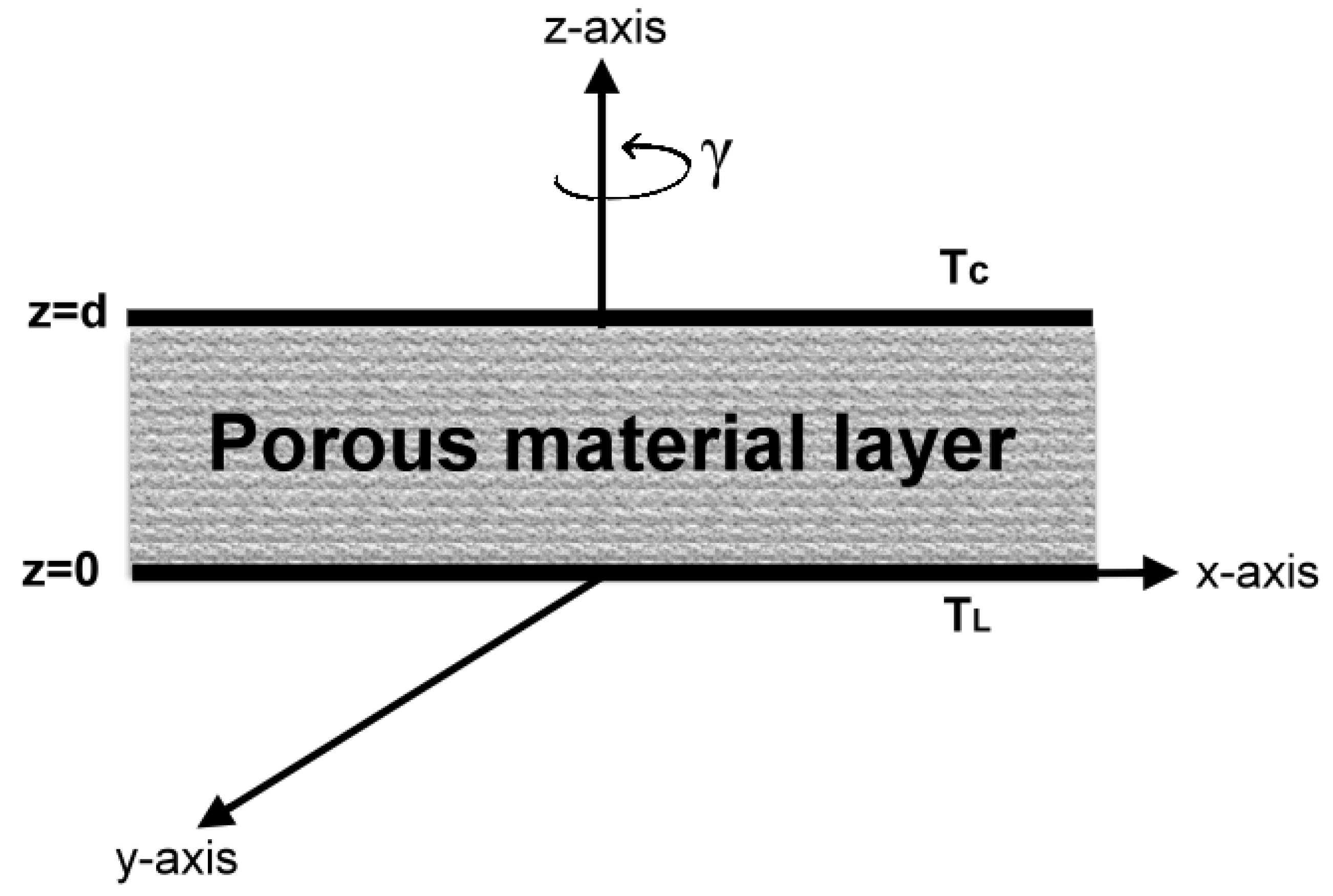
2. Basic Equations

Consider a rotating porous material layer that is located between the two planes $z=0$ and $z=d$ and that has been saturated with fluid as shown in Figure 1 below.

The problem can be represented as follows

$$T_s=T_f=T_L,C=C_L,z=0;T_s=T_f=T_U,C=C_U,z=d.$$

(1)

The equations are:

$$\begin{array}{c}{v}_i=-\frac{K}{\mu }{p}_{,i}-\nu \left|\mathbf{v}\right|v_i+\hat{\nu }\Delta v_i-\frac{K\mathrm{g}{\rho }_f}{\mu }[1-{\alpha }_t(T_f-T_L)+{\alpha }_c(C-C_L)]k_i-\frac{2}{\epsilon }{(\gamma \times \mathbf{v})}_i,\\ v_{i,i}=0,\\ \epsilon {\left(\rho c\right)}_f{T}_{,t}^f+{\left(\rho c\right)}_f{v}_i{T}_{,i}^f=\epsilon {\kappa }_f\Delta T_f+h(T_s-T_f),\\ (1-\epsilon ){\left(\rho c\right)}_s{T}_{,t}^s=(1-\epsilon ){\kappa }_s\Delta T_s-h(T_s-T_f),\\ \epsilon C_{,t}+v_i{C}_{,i}=\epsilon {\kappa }_c\Delta C,\end{array}$$

(2)

where $\Delta$ is the Laplace operator in 3-dimensions. $v_i,p,C,T_s$ and $T_f$ denote velocity, pressure, concentration of salt, temperature of the solid and temperature of the fluid, respectively. The terms $K,\mu ,\mathrm{g},\rho ,\epsilon ,{\alpha }_t,{\alpha }_c,c,h,{\kappa }_f,{\kappa }_s,{\kappa }_c,\gamma ,\nu$ and $\widehat{\nu }$ denote permeability, dynamic viscosity, gravity, density, porosity, thermal expansion coefficient, solute expansion coefficient, specific heat at constant pressure, inter-phase heat transfer coefficient, thermal conductivity of the fluid expansion coefficient, thermal conductivity of the solid, salt diffusivity, angular velocity of rotation, Forchheimer coefficient and Brinkman coefficient, respectively.

Throughout this paper, we will use both of the standard indicial and Einstein notations, and $k_i=(0,0,1)$.

Let us assume that the domain $D_E=\{(x,y)\in {\mathbb{R}}^2\}\times \{z\in (-1,1)\}\times \{t>0\}$. It is obvious that the equations of (1) hold in $D_E$, and assume that $B_s=(\overline{v_i},\overline{p},\overline{T_f},\overline{T_s},\overline{C})$ denote the solution of the initial steady state of the system, such that the fluid flow is vanished, $\overline{v_i}\equiv 0$, and assume also that these solutions are in terms of only z, such that:

$$\overline{T_s}=\overline{T_f}=-{\beta }_{t}z+T_L,\overline{C}=-{\beta }_{c}z+C_L,$$

(3)

where ${\beta }_t=\frac{T_U-T_L}{d}$, ${\beta }_c=\frac{C_U-C_L}{d}$, $\overline{p}$ which is called the steady pressure, and it is given by (2)₁ and can be reduced to

$${\overline{p}}_{,i}=\mathrm{g}{\rho }_f[1-{\alpha }_t({\overline{T}}_f-T_L)+{\alpha }_c(\overline{C}-C_L)]k_i,$$

(4)

To understand how the stability in (2) works, we introduce the perturbation $(u_i,\pi ,\theta ,\psi ,\varphi )$ to the steady solutions $(\overline{v_i},\overline{p},\overline{T_f},\overline{T_s},\overline{C})$, such that

$$v_i=\overline{v_i}+u_i,p=\overline{p}+\pi ,T_f=\overline{T_f}+\theta ,T_s=\overline{T_s}+\psi ,\mathrm{and}C=\overline{C}+\varphi$$

Using the equations in (3) and in (4), the system can be introduced as the following

$$\begin{array}{c}{u}_i=-\frac{K}{\mu }{\pi }_{,i}-\nu \left|\mathbf{u}\right|u_i+\hat{\nu }\Delta u_i+\frac{{\rho }_{f}K\mathrm{g}{\alpha }_t}{\mu }\theta k_i-\frac{{\rho }_{f}K\mathrm{g}{\alpha }_c}{\mu }\varphi k_i-\frac{2}{\epsilon }{(\gamma \times \mathbf{u})}_i,\\ u_{i,i}=0,\\ \epsilon {\left(\rho c\right)}_f{\theta }_{,t}+{\left(\rho c\right)}_f{u}_i{\theta }_{,i}={\left(\rho c\right)}_f{\beta }_{t}w+\epsilon {\kappa }_f\Delta \theta +h(\psi -\theta ),\\ (1-\epsilon ){\left(\rho c\right)}_s{\psi }_{,t}=(1-\epsilon ){\kappa }_s\Delta \psi -h(\psi -\theta ),\\ \epsilon {\varphi }_{,t}+u_i{\varphi }_{,i}={\beta }_{c}w+\epsilon {\kappa }_c\Delta \varphi .\end{array}$$

(5)

Let us consider now the variables with no dimensions that have the following scales

$$x_i=x_i^{*}d,t=\frac{{\left(\rho c\right)}_f{d}^2}{{\kappa }_f}{t}^{*},u_i=U{u}_i^{*},\pi =\frac{U\mu d}{K}{\pi }^{*},\theta =T^{♯}{\theta }^{*},\psi =T^{♯}{\psi }^{*},\varphi =T_{\varphi }^{♯}{\varphi }^{*},\tau =\frac{2\gamma }{\epsilon },$$

$$U=\frac{\epsilon {\kappa }_f}{{\left(\rho c\right)}_{f}d},{\kappa }_c=\frac{{\kappa }_f}{{\left(\rho c\right)}_f},M=\frac{h{d}^2}{\epsilon {\kappa }_f},\mathcal{F}=\nu U,B=\frac{\hat{\nu }}{d^2},\mathcal{A}=\frac{{\left(\rho c\right)}_s{\kappa }_f}{{\left(\rho c\right)}_f{\kappa }_s},\lambda =\frac{\epsilon {\kappa }_f}{(1-\epsilon ){\kappa }_s},$$

$$T^{♯}=Ud\sqrt{\frac{\mu {\beta }_t{c}_f}{\epsilon {\kappa }_f\mathrm{g}{\alpha }_{t}K}},T_{\varphi }^{♯}=Ud\sqrt{\frac{\mu {\beta }_c{c}_f}{\epsilon {\kappa }_f\mathrm{g}{\alpha }_{c}K}},R_t={\rho }_{f}d\sqrt{\frac{{\alpha }_t{\beta }_t{c}_f\mathrm{g}K}{\mu \epsilon {\kappa }_f}},R_c={\rho }_{f}d\sqrt{\frac{{\alpha }_c{\beta }_c{c}_f\mathrm{g}K}{\mu \epsilon {\kappa }_f}}.$$

Here $R_t$ and $R_c$ are the numbers of Rayleigh (dimensionless numbers), and $\tau$ is the Taylor-Darcy number. Therefore, the equations of the system of no-dimension can be given as

$$\begin{array}{c}{u}_i=-{\pi }_{,i}-\mathcal{F}\left|\mathbf{u}\right|u_i+B\Delta u_i+R_t\theta k_i-R_c\varphi k_i-(\tau \times \mathbf{u}),\\ u_{i,i}=0,\\ {\theta }_{,t}+u_i{\theta }_{,i}=R_{t}w+\Delta \theta +M(\psi -\theta ),\\ \mathcal{A}{\psi }_{,t}=\Delta \psi -\lambda M(\psi -\theta ),\\ {\varphi }_{,t}+u_i{\varphi }_{,i}=R_{c}w+\Delta \varphi ,\end{array}$$

(6)

where $\mathcal{F}$ and B are the Forchheimer and Brinkman coefficients, respectively, and the boundary conditions are given by the following

$$u_i=0,\theta =0,\psi =0,\varphi =0,\mathrm{on}z=0,1.$$

(7)

3. Linear Instability

To obtain the threshold for linear instability case, we neglect the nonlinear terms from system (6). Since we have here a linearity, one can find solutions for the form $u_i(\mathbf{x},t)=u_i\left(\mathbf{x}\right)e^{\sigma t},\theta (\mathbf{x},t)=\theta \left(\mathbf{x}\right)e^{\sigma t},\psi (\mathbf{x},t)=\psi \left(\mathbf{x}\right)e^{\sigma t}$ and $\varphi (\mathbf{x},t)=\varphi \left(\mathbf{x}\right)e^{\sigma t},$ such that $\sigma \in \mathbb{C}$. Thus, we end up having the following system

$$\begin{array}{c}{u}_i=-{\pi }_{,i}+B\Delta u_i+R_t\theta k_i-R_c\varphi k_i-(\tau \times \mathbf{u}),\\ u_{i,i}=0,\\ \sigma \theta =R_{t}w+\Delta \theta +M(\psi -\theta ),\\ \mathcal{A}\sigma \psi =\Delta \psi -\lambda M(\psi -\theta ),\\ \sigma \varphi =R_{c}w+\Delta \varphi .\end{array}$$

(8)

Now, taking the third components of the $curl$ and double $curl$ of Equation (8)₁ in system (8), leads to

$$\begin{array}{c}\phi =\tau w_z,\\ \Delta w=B{\Delta }^{2}w+R_t{\Delta }^{*}\theta -R_c{\Delta }^{*}\varphi -\tau \frac{\partial \phi }{\partial z},\\ u_{i,i}=0,\\ \sigma \theta =R_{t}w+\Delta \theta +M(\psi -\theta ),\\ \mathcal{A}\sigma \psi =\Delta \psi -\lambda M(\psi -\theta ),\\ \sigma \varphi =R_{c}w+\Delta \varphi .\end{array}$$

(9)

Here ${\Delta }^{*}=\frac{{\partial }^2}{\partial x^2}+\frac{{\partial }^2}{\partial y^2}$ and $\phi =\mathbf{k}·\nabla \times \mathbf{u}$ is the third component of the vorticity. Substituting (9)₁ into (9)₂, we obtain

$$\begin{array}{c}\Delta w=B{\Delta }^{2}w+R_t{\Delta }^{*}\theta -R_c{\Delta }^{*}\varphi -{\tau }^2{w}_{zz},\\ u_{i,i}=0,\\ \sigma \theta =R_{t}w+\Delta \theta +M(\psi -\theta ),\\ \mathcal{A}\sigma \psi =\Delta \psi -\lambda M(\psi -\theta ),\\ \sigma \varphi =R_{c}w+\Delta \varphi .\end{array}$$

(10)

Now, we consider the so-called “normal mode” of the representation $w=W\left(z\right)h(x,y)$, $\theta =\mathrm{\Theta }\left(z\right)h(x,y)$, $\psi =\mathrm{\Psi }\left(z\right)h(x,y)$ and $\varphi =\mathrm{\Phi }\left(z\right)h(x,y)$, such that $h(x,y)$ is a plan-form that tiles the plane $(x,y)$ with ${\Delta }^{*}h=-a^{2}h$.

Applying the previous represented mode, equations in (10) yield

$$\begin{array}{c}(D^2-a^2)W=B{(D^2-a^2)}^{2}W-a^2{R}_t\mathrm{\Theta }+a^2{R}_c\mathrm{\Phi }-{\tau }^2{D}^{2}W,\\ \sigma \mathrm{\Theta }=(D^2-a^2)\mathrm{\Theta }+R_{t}W+M(\mathrm{\Psi }-\mathrm{\Theta }),\\ \sigma \mathcal{A}\mathrm{\Psi }=(D^2-a^2)\mathrm{\Psi }-\lambda M(\mathrm{\Psi }-\mathrm{\Theta }),\\ \sigma \mathrm{\Phi }=(D^2-a^2)\mathrm{\Phi }+R_{c}W,\end{array}$$

(11)

and the boundary conditions are

$$W=0,\mathrm{\Theta }=0,\mathrm{\Psi }=0,\mathrm{\Phi }=0,\mathrm{at}z=0,1.$$

(12)

Hence, letting

$$\mathfrak{D}=D^2-a^2,{\mathfrak{D}}_1=\mathfrak{D}-M-\sigma ,{\mathfrak{D}}_2=\mathfrak{D}-\lambda M-\sigma \mathcal{A},{\mathfrak{D}}_3={\mathfrak{D}}_1{\mathfrak{D}}_2-\lambda M^2,\mathrm{and}{\mathfrak{D}}_4=\mathfrak{D}-\sigma .$$

Thus, from (11)₂, (11)₃ and (11)₄, and by applying the above assumptions, we obtain

$${\mathfrak{D}}_1\mathrm{\Theta }=-R_{t}W-M\mathrm{\Psi },{\mathfrak{D}}_2\mathrm{\Psi }=-\lambda M\mathrm{\Theta },{\mathfrak{D}}_3\mathrm{\Theta }=-R_t{\mathfrak{D}}_{2}W\mathrm{and}{\mathfrak{D}}_4\mathrm{\Phi }=-R_{c}W.$$

(13)

Now, multiplying Equation (11)₁ by ${\mathfrak{D}}_3$ and ${\mathfrak{D}}_4$, yields

$${\mathfrak{D}}_3{\mathfrak{D}}_4\mathfrak{D}W=B{\mathfrak{D}}_3{\mathfrak{D}}_4{\mathfrak{D}}^{2}W-a^2{R}_t{\mathfrak{D}}_3{\mathfrak{D}}_4\mathrm{\Theta }+a^2{R}_c{\mathfrak{D}}_3{\mathfrak{D}}_4\mathrm{\Phi }-{\tau }^2{\mathfrak{D}}_3{\mathfrak{D}}_4{D}^{2}W$$

(14)

With $\sigma =0$, (13) is reduced to

$$\begin{array}{c}({\mathfrak{D}}^4-M[1+\lambda ]{\mathfrak{D}}^3)W=B({\mathfrak{D}}^5-M[1+\lambda ]{\mathfrak{D}}^4)W+a^2{R}_t^2({\mathfrak{D}}^2-\lambda M\mathfrak{D})W\\ -a^2{R}_c^2({\mathfrak{D}}^2-M[1+\lambda ]\mathfrak{D})W-{\tau }^2({\mathfrak{D}}^3-M[1+\lambda ]{\mathfrak{D}}^2)D^{2}W.\end{array}$$

(15)

Since the boundary condition $W=0$ is represented on $z=0,1$, one can rewrite W as series of the sin function, such that $\sin \left(\eta \right)$, where $\eta =n\pi z$. Next, with $\mathrm{\Lambda }=\frac{\eta }{z^2}+a^2$, and a is the number of waves in the series in (15), one can obtain

$$R_t^2=\frac{\{{\mathrm{\Lambda }}^2+B{\mathrm{\Lambda }}^3+{\tau }^2{n}^2{\pi }^2\mathrm{\Lambda }+a^2{R}_c^2\}(\mathrm{\Lambda }+M[1+\lambda ])}{a^2(\mathrm{\Lambda }-\lambda M)}.$$

(16)

Then, minimizing $R_t^2$ with respect to $a^2$, we obtain

$$C_5{\mathrm{\Lambda }}^5+C_4{\mathrm{\Lambda }}^4+C_3{\mathrm{\Lambda }}^3+C_2{\mathrm{\Lambda }}^2+C_1\mathrm{\Lambda }+C_0=0,$$

(17)

where

$$C_5=2B,C_4=1+Bk+2HB,C_3=2H(1+Bk)-4\lambda {\pi }^{2}M-R_c^2,$$

$$C_2=2(L+k)-(kL-R_c^2{\pi }^2)-3{\pi }^2\lambda M(1+Bk)-2k{R}_c^2,$$

$$C_1=-2(L+k)+2k{R}_c^2{\pi }^2-R_c^2-Hk{R}_c^2,$$

$$C_0={\pi }^2\lambda M(kL-R_c^2{\pi }^2)-Hk{R}_c^2{\pi }^2,$$

$$k=M(1+\lambda ),L={\tau }^2{\pi }^2\mathrm{and}H=\lambda M-{\pi }^2.$$

As finding the zeros of Equation (17) analytically is almost impossible, we use some iterative methods for solving nonlinear equations such as Newton Raphson (NR), Bisection, and many other methods that can be seen in [36]. In fact, we use here the Newton–Raphson iterative method (NR) to solve the equation in (17) as we already tried with many different methods, but the results of NR method are more accurate and method converges to the solutions faster than the methods with fewer iterations. The following steps show how we use NR method. First, let

$$\mathcal{P}\left(\mathrm{\Lambda }\right)=c_5{\mathrm{\Lambda }}^5+c_4{\mathrm{\Lambda }}^4+c_3{\mathrm{\Lambda }}^3+c_2{\mathrm{\Lambda }}^2+c_1\mathrm{\Lambda }+c_0=0,$$

Next, we can create a sequence of initial solutions by using the following formula:

$${\mathrm{\Lambda }}_n={\mathrm{\Lambda }}_{n-1}-\frac{\mathcal{P}\left({\mathrm{\Lambda }}_{n-1}\right)}{{\mathcal{P}}^{\prime }\left({\mathrm{\Lambda }}_{n-1}\right)},$$

where we select ${\mathrm{\Lambda }}_0={\pi }^2$. In fact, the tolerance here is $\gamma >0$ and by repeating the iterations we can keep creating the solutions ${\mathrm{\Lambda }}_1,....,{\mathrm{\Lambda }}_N$ until we satisfy the condition below:

$$|f\left({\mathrm{\Lambda }}_n\right)|<\gamma ={10}^{-10}.$$

(18)

Moreover, we can use another method such as the fixed-point method (FP), where can write the previous mentioned equation as below:

$$\mathrm{\Lambda }=\frac{1}{\sqrt[5]{c_5}}{\left(-c_4{\mathrm{\Lambda }}^4-c_3{\mathrm{\Lambda }}^3-c_2{\mathrm{\Lambda }}^2-c_1\mathrm{\Lambda }-c_0\right)}^{1/5}.$$

(19)

Then, with ${\mathrm{\Lambda }}_0={\pi }^2$, one may use the formula below:

$${\mathrm{\Lambda }}_n=\frac{1}{\sqrt[5]{c_5}}{\left(-c_4{\mathrm{\Lambda }}_{n-1}^4-c_3{\mathrm{\Lambda }}_{n-1}^3-c_2{\mathrm{\Lambda }}_{n-1}^2-c_1{\mathrm{\Lambda }}_{n-1}-c_0\right)}^{1/5}.$$

(20)

One may also use here the tolerance $\gamma >0$ and by repeating the iterations we can keep creating the solutions ${\mathrm{\Lambda }}_1,....,{\mathrm{\Lambda }}_N$ until we satisfy the condition below:

$$|{\mathrm{\Lambda }}_n-{\mathrm{\Lambda }}_{n-1}|<\gamma ={10}^{-10}.$$

(21)

4. Nonlinear Energy Stability Theory

4.1. Nonlinear Stability Analysis with Forchheimer Coefficient $\mathcal{F}=0$

Before developing the nonlinear energy stability analysis, we can start by taking the third component of Equation (6)₁ in the system (6), which will lead to

$$\begin{array}{c}\phi =\tau w_z,\\ \Delta w=B{\Delta }^{2}w+R_t{\Delta }^{*}\theta -R_c{\Delta }^{*}\varphi -\tau \frac{\partial \phi }{\partial z},\end{array}$$

(22)

substituting (22)₁ into (22)₂, we obtain

$$\Delta w=B{\Delta }^{2}w+R_t{\Delta }^{*}\theta -R_c{\Delta }^{*}\varphi -{\tau }^2{w}_{zz}.$$

(23)

Let us suppose that V represents the period cell, $\parallel ·\parallel$ represents the norm on $L^2\left(V\right)$, and $(·,·)$ represents the inner product on $L^2\left(V\right)$. Niow, multiplying (23) by w, (6)${}_3$ by $\theta$, (6)${}_4$ by ${\lambda }^{-1}\psi$ and (6)₅ by $\varphi$ and integrating over V, yield

$$\begin{array}{c}0=-{\parallel \nabla w\parallel }^2-{\tau }^2\parallel w_z{\parallel }^2-B{\parallel \Delta w\parallel }^2+R_t({\nabla }^{*}\theta ,{\nabla }^{*}w)-R_c({\nabla }^{*}\varphi ,{\nabla }^{*}w),\\ \frac{d}{dt}\frac{1}{2}{\parallel \theta \parallel }^2=R_t(w,\theta )-{\parallel \nabla \theta \parallel }^2+M(\theta ,\psi -\theta ),\\ \frac{d}{dt}\frac{\mathcal{A}}{2\lambda }{\parallel \psi \parallel }^2=-{\lambda }^{-1}{\parallel \nabla \psi \parallel }^2-M(\psi ,\psi -\theta ),\\ \frac{d}{dt}\frac{1}{2}{\parallel \varphi \parallel }^2=R_c(w,\varphi )-{\parallel \nabla \varphi \parallel }^2.\end{array}$$

(24)

Multiply (24)₁ by ${\lambda }_1$ and (24)₄ by ${\lambda }_2$ and define $E,\mathcal{I}$ and $\mathcal{D}$ by

$$\begin{array}{c}E\left(t\right)=\frac{1}{2}{\parallel \theta \parallel }^2+\frac{\mathcal{A}}{2\lambda }{\parallel \psi \parallel }^2+\frac{{\lambda }_2}{2}{\parallel \varphi \parallel }^2,\\ \mathcal{I}={\lambda }_1{R}_t({\nabla }^{*}\theta ,{\nabla }^{*}w)+R_t(w,\theta )-{\lambda }_1{R}_c({\nabla }^{*}\varphi ,{\nabla }^{*}w)+R_c(w,\varphi ),\\ \mathcal{D}={\lambda }_1{\parallel \nabla w\parallel }^2+{\tau }^2{\lambda }_1\parallel w_z{\parallel }^2+B{\lambda }_1{\parallel \Delta w\parallel }^2+{\parallel \nabla \theta \parallel }^2+{\lambda }^{-1}{\parallel \nabla \psi \parallel }^2+{\lambda }_2{\parallel \nabla \varphi \parallel }^2+M{\parallel \theta -\psi \parallel }^2,\end{array}$$

(25)

from adding (24)₁–(24)₄, we obtain

$$\frac{dE}{dt}=\mathcal{I}-\mathcal{D}\le -\mathcal{D}(1-\frac{1}{{\rm Y}}),$$

(26)

where

$$\frac{1}{{\rm Y}}=\underset{\mathcal{H}}{max}\frac{\mathcal{I}}{\mathcal{D}}.$$

(27)

If ${\rm Y}>1$, then with substituting $\pi$ as the constant in poincarés inequality, we can see that

$$\mathcal{D}\ge c(\parallel \theta {\parallel }^2+\parallel \psi {\parallel }^2+\parallel \varphi {\parallel }^2)=cE,$$

where $c=min\{2\pi ,2\pi \lambda {\mathcal{A}}^{-1},2\pi {\lambda }_2^{-1}\}$, from integrating (26) with $\gamma =c(1-\frac{1}{{\rm Y}})$, we have

$$E\left(t\right)\le E\left(0\right)e^{-\gamma t}\Rightarrow E\left(t\right)\to 0\mathrm{as}t\to \infty \mathrm{at}\mathrm{least}\mathrm{exponentially}.$$

From Equation (6)₁ ($\mathcal{F}=0$), with substituting $\mu$ as the constant in the poincarés inequality, one could show that

$${\parallel \mathbf{u}\parallel }^2\le -\mu B{\parallel \mathbf{u}\parallel }^2+R_t(w,\theta )-R_c(w,\varphi ),$$

by using Youngs inequality, we obtain

$${(1+\mu B)\parallel \mathbf{u}\parallel }^2\le \frac{R_t^2}{2}{\parallel \theta \parallel }^2+\frac{R_c^2}{2}{\parallel \varphi \parallel }^2+{\parallel w\parallel }^2,$$

hence,

$${\parallel \mathbf{u}\parallel }^2\le \frac{R_t^2}{2\mu B}{\parallel \theta \parallel }^2+\frac{R_c^2}{2\mu B}{\parallel \varphi \parallel }^2.$$

Therefore, ${\rm Y}>1$ also ensures the exponential decay $\parallel \mathbf{u}\parallel .$ One can show that ${\rm Y}>1$ is equivalent to $R<R_E$, where $R_E$ is the value of R for which ${\rm Y}=1$. This value of $R_E$ is the nonlinear stability threshold.

To solve the maximum problem (27), we study the Euler Lagrange equations which can be found from

$$R_E\delta \mathcal{I}-\delta \mathcal{D}=0.$$

(28)

Thus, the equations of Euler Lagrange appear from variational problem (28), are

$$\begin{array}{c}2{\lambda }_1(\Delta w-B{\Delta }^{2}w+{\tau }^2{w}_{zz})+R_t(\theta -{\lambda }_1{\Delta }^{*}\theta )+R_c({\lambda }_1{\Delta }^{*}\varphi +{\lambda }_2\varphi )={\zeta }_{,i}\\ 2(\Delta \theta -M\theta )+R_t(w-{\lambda }_1{\Delta }^{*}w)+2M\psi =0,\\ {\lambda }^{-1}\Delta \psi -M\psi +M\theta =0,\\ 2{\lambda }_2\Delta \varphi +R_c({\lambda }_{2}w+{\lambda }_1{\Delta }^{*}w)=0.\end{array}$$

(29)

Now, eliminating the Lagrange multiplier $\zeta$, and representing the normal mode and notation as described in Section 3, system (29), yields

$$\begin{array}{c}(D^2-a^2)W-B{(D^2-a^2)}^{2}W+{\tau }^2{D}^{2}W+\frac{R_t(1+a^2{\lambda }_1)}{2{\lambda }_1}\mathrm{\Theta }+\frac{R_c({\lambda }_2-a^2{\lambda }_1)}{2{\lambda }_1}\mathrm{\Phi }=0,\\ (D^2-a^2-M)\mathrm{\Theta }+\frac{R_t(1+a^2{\lambda }_1)}{2}W+M\mathrm{\Psi }=0,\\ (D^2-a^2-\lambda M)\mathrm{\Psi }+\lambda M\mathrm{\Theta }=0,\\ (D^2-a^2)\mathrm{\Phi }+\frac{R_c({\lambda }_2-a^2{\lambda }_1)}{2{\lambda }_2}W=0.\end{array}$$

(30)

Now, one may evaluate the critical Rayleigh number (CRN) by using the following

$$R_E=\underset{{\lambda }_1,{\lambda }_2}{max}\underset{a^2}{min}{R}_t^2(a^2,{\lambda }_1,{\lambda }_2).$$

4.2. Nonlinear Stability Analysis with Taylor-Darcy Number $\tau =0$ $(\mathcal{F}\ne 0)$

Multiply, (6)₁ by $u_i$, (6)₃ by $\theta$, (6)₄ by ${\lambda }^{-1}\psi$ and (6)₅ by $\varphi$ and integrating over V, we obtain

$$\begin{array}{c}0=-{\parallel \mathbf{u}\parallel }^2-{\mathcal{F}\parallel \mathbf{u}\parallel }_3^3-B{\parallel \nabla \mathbf{u}\parallel }^2+R_t(w,\theta )-R_c(w,\varphi ),\\ \frac{d}{dt}\frac{1}{2}{\parallel \theta \parallel }^2=R_t(w,\theta )-{\parallel \nabla \theta \parallel }^2+M(\theta ,\psi -\theta ),\\ \frac{d}{dt}\frac{\mathcal{A}}{2\lambda }{\parallel \psi \parallel }^2=-{\lambda }^{-1}{\parallel \nabla \psi \parallel }^2-M(\psi ,\psi -\theta ),\\ \frac{d}{dt}\frac{1}{2}{\parallel \varphi \parallel }^2=R_c(w,\varphi )-{\parallel \nabla \varphi \parallel }^2,\end{array}$$

(31)

where ${\parallel ·\parallel }_3$ denotes the $L^3\left(V\right)$. Let us assume now that both of ${\lambda }_1$ and ${\lambda }_2$ are positive parameters. Therefore, by multiplying (31)₁ by ${\lambda }_1$, (31)₄ by ${\lambda }_2$ and adding these two equations with (31)₂ and (31)₃, we obtain

$$\frac{dE}{dt}=\mathcal{I}-\mathcal{D}-{\lambda }_1\mathcal{F}{\parallel \mathbf{u}\parallel }_3^3\le \mathcal{I}-\mathcal{D},$$

where $E,\mathcal{I}$ and $\mathcal{D}$ are given by

$$\begin{array}{c}E\left(t\right)=\frac{1}{2}{\parallel \theta \parallel }^2+\frac{\mathcal{A}}{2\lambda }{\parallel \psi \parallel }^2+\frac{{\lambda }_2}{2}{\parallel \varphi \parallel }^2,\\ \mathcal{I}=R_t([1+{\lambda }_1]w,\theta )+R_c([{\lambda }_2-{\lambda }_1]w,\varphi ),\\ \mathcal{D}={\lambda }_1{\parallel \mathbf{u}\parallel }^2+{\lambda }_1{B\parallel \nabla \mathbf{u}\parallel }^2+{\parallel \nabla \theta \parallel }^2+{\lambda }^{-1}{\parallel \nabla \psi \parallel }^2+{\lambda }_2{\parallel \nabla \varphi \parallel }^2+M{\parallel \theta -\psi \parallel }^2,\end{array}$$

(32)

With some mathematical simplifications, we obtain

$$\frac{dE}{dt}=-\mathcal{D}(1-\frac{1}{R_E}),$$

(33)

where

$$\frac{1}{R_E}=\underset{\mathcal{H}}{max}\frac{\mathcal{I}}{\mathcal{D}},$$

(34)

such that $\mathcal{H}$ is the space of admissible functions.

In fact, if $R_E>1$ then substituting $\pi$ as the constant in poincarés inequality, one can obtain

$$\mathcal{D}\ge \alpha (\parallel \theta {\parallel }^2+\parallel \psi {\parallel }^2+\parallel \varphi {\parallel }^2)=\alpha E,$$

where $\alpha =min\{2\pi ,2\pi \lambda {\mathcal{A}}^{-1},2\pi {\lambda }_2^{-1}\}$. Now integrating (33) with $\gamma =\alpha (1-\frac{1}{R_E})$, yields

$$E\left(t\right)\le E\left(0\right)e^{-\gamma t}\Rightarrow E\left(t\right)\to 0\mathrm{as}t\to \infty \mathrm{at}\mathrm{least}\mathrm{exponentially}.$$

To obtain decay of $\mathbf{u}$, we note from Equation (31)₁ with the aid of Youngs inequality

$${\parallel \mathbf{u}\parallel }^2+{\mathcal{F}\parallel \mathbf{u}\parallel }_3^3+B{\parallel \nabla \mathbf{u}\parallel }^2=R_t(w,\theta )-R_c(w,\varphi )$$

$$\le R_t^2{\parallel \theta \parallel }^2+R_c^2{\parallel \varphi \parallel }^2+\frac{1}{2}{\parallel w\parallel }^2$$

$$\le R_t^2{\parallel \theta \parallel }^2+R_c^2{\parallel \varphi \parallel }^2+\frac{1}{2}{\parallel \mathbf{u}\parallel }^2.$$

Then, the decay of $\mathbf{u}$ is clearly obtained.

Since the global stability has been already established, we can study the maximum problem (34) keeping in mind its condition as $R_E>1$. In fact, we could solve this maximization problem by studying the equations of Euler Lagrange which can be obtained from the following

$$R_E\delta \mathcal{I}-\delta \mathcal{D}=0.$$

Now, by using the above equation and the values of both $\delta \mathcal{I}$ and $\delta \mathcal{D}$, one can obtain the following equations

$$\begin{array}{c}2{\lambda }_1{u}_i-2{\lambda }_{1}B\Delta u_i+R_t(1+{\lambda }_1)\theta k_i+R_c({\lambda }_2-{\lambda }_1)\varphi k_i={\varsigma }_{,i},\\ 2\Delta \theta +R_t(1+{\lambda }_1)w-2M\theta +2M\psi =0,\\ {\lambda }^{-1}\Delta \psi +M\theta -M\psi =0,\\ 2{\lambda }_2\Delta \varphi +R_c({\lambda }_2-{\lambda }_1)w=0,\end{array}$$

(35)

The above equations in (35) are called the Euler Lagrange equations, where ${\varsigma }_{,i}$ represents the Lagrange multiplier. Now, by taking the third component in (35)₁, one can remove the Lagrange multiplier. Thus, we obtain

$$\begin{array}{c}2{\lambda }_1\Delta w-2{\lambda }_{1}B{\Delta }^{2}w+R_t(1+{\lambda }_1){\Delta }^{*}\theta +R_c({\lambda }_2-{\lambda }_1){\Delta }^{*}\varphi =0,\\ 2\Delta \theta +R_t(1+{\lambda }_1)w-2M\theta +2M\psi =0,\\ {\lambda }^{-1}\Delta \psi +M\theta -M\psi =0,\\ 2{\lambda }_2\Delta \varphi +R_c({\lambda }_2-{\lambda }_1)w=0.\end{array}$$

(36)

Introducing the normal mode representations, then, system (36) becomes

$$\begin{array}{c}(D^2-a^2)W-B{(D^2-a^2)}^{2}W-\frac{a^2{R}_t(1+{\lambda }_1)}{2{\lambda }_1}\mathrm{\Theta }-\frac{a^2{R}_c({\lambda }_2-{\lambda }_1)}{2{\lambda }_1}\mathrm{\Phi }=0,\\ (D^2-a^2-M)\mathrm{\Theta }+\frac{R_t(1+{\lambda }_1)}{2}W+M\mathrm{\Psi }=0,\\ (D^2-a^2-\lambda M)\mathrm{\Psi }+\lambda M\mathrm{\Theta }=0,\\ (D^2-a^2)\mathrm{\Phi }+\frac{R_c({\lambda }_2-{\lambda }_1)}{2{\lambda }_2}W=0.\end{array}$$

(37)

Now, one my evaluate the critical Rayleigh number (CRN) by using the following

$$R_E=\underset{{\lambda }_1,{\lambda }_2}{max}\underset{a^2}{min}{R}_t^2(a^2,{\lambda }_1,{\lambda }_2).$$

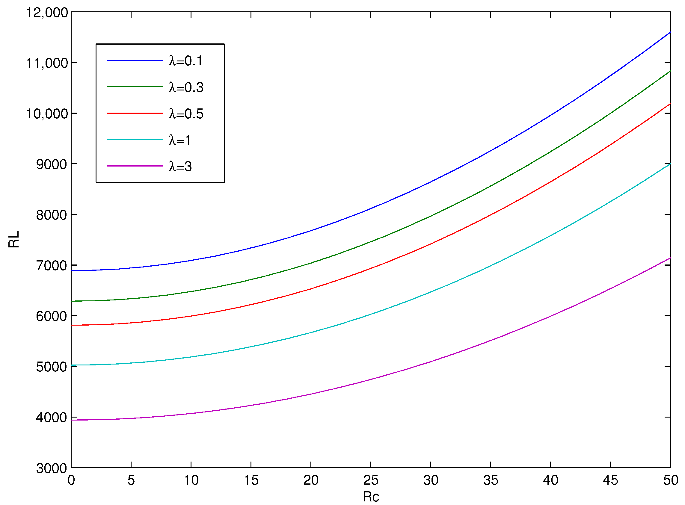
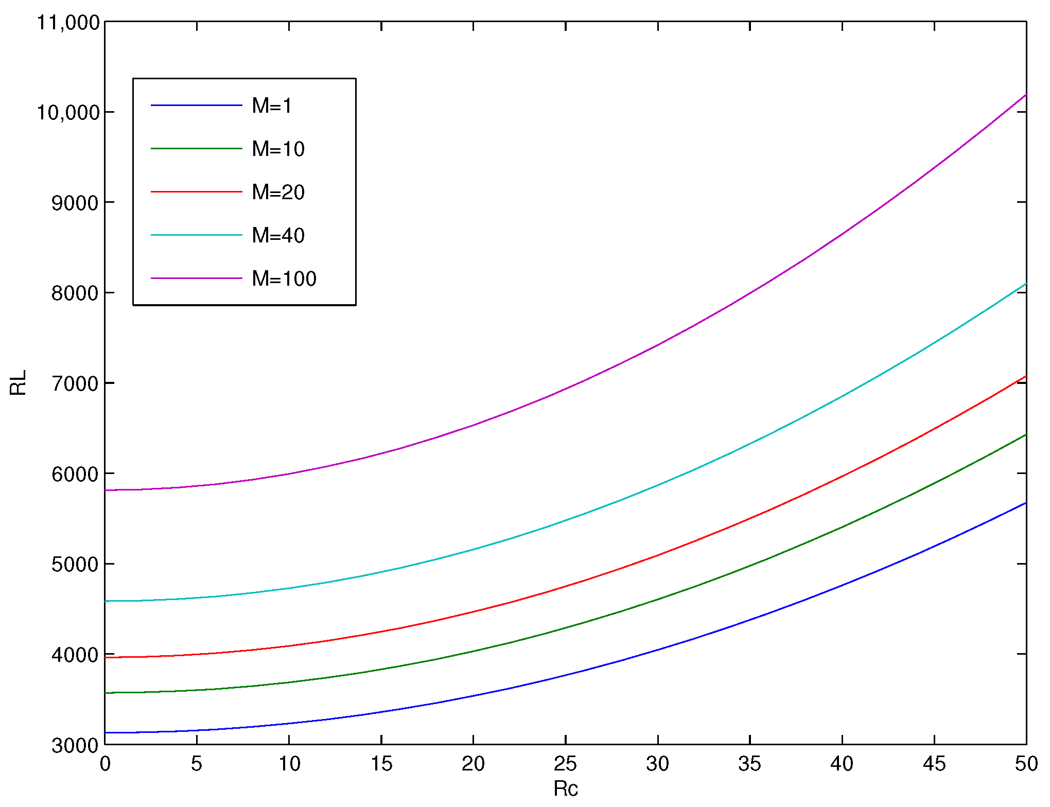
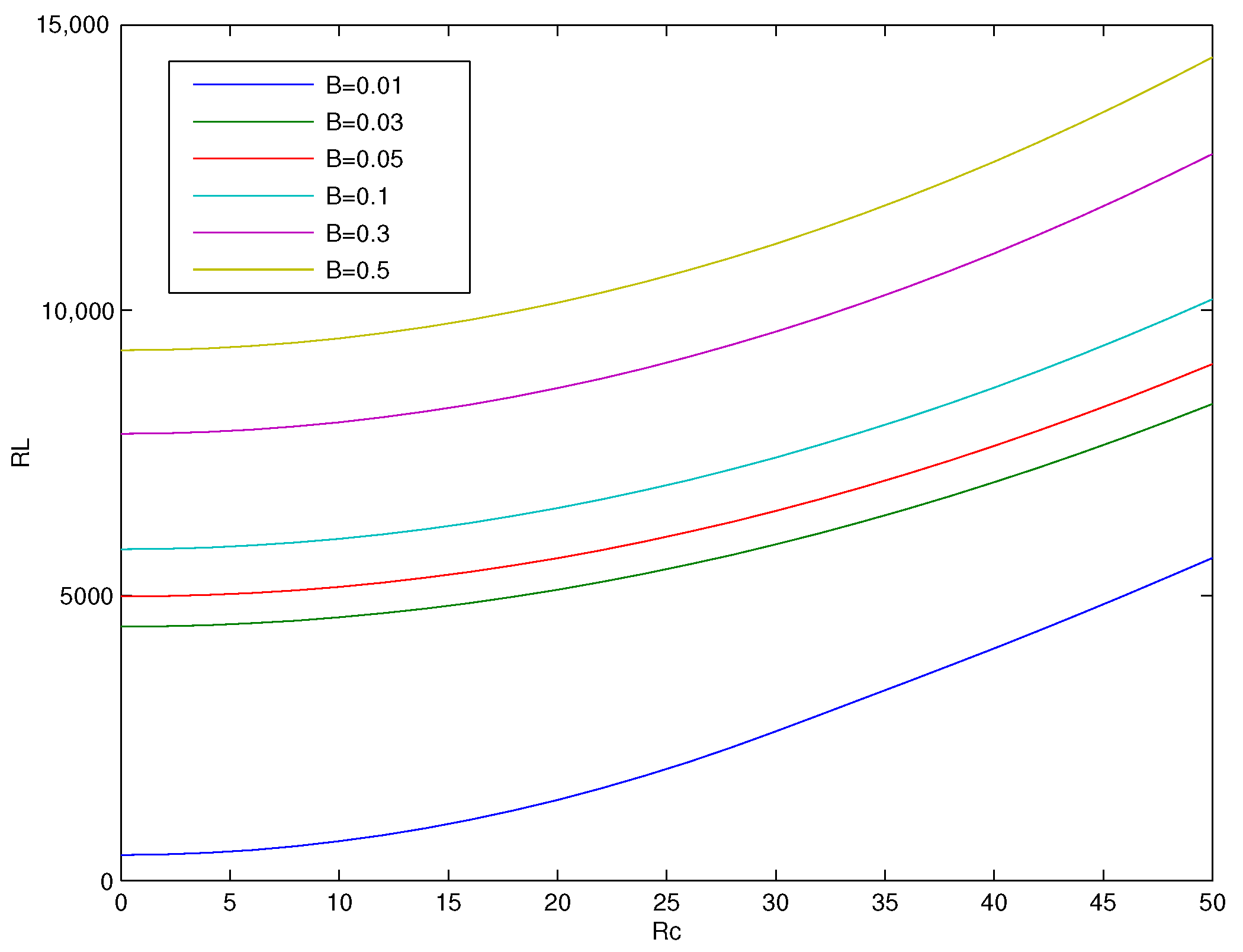
5. Discussion of Results

For the validation of the proposed work, we present in this section some experimental examples and focus on the numerical solutions of the instability of the linear case and the stability of the nonlinear case. The numerical solutions of the systems in (11) (the linear instability), with respect to the stationary and oscillatory convection cases. The results are reported when $M=100,\lambda =0.5,\tau =20$ and $B=0.1$. Furthermore, we discuss the different values of $\lambda ,M,B,\tau$ and $R_c$ in Figure 2, Figure 3, Figure 4 and Figure 5. Chebyshev collocation method has been used for solving the systems of eigenproblems (11), (30) and (37). More information about these types of systems can be seen in [21,22,23,24,37,38,39]. The solutions are then presented in

Table 1. Critical thermal Rayleigh number $R_L$ against $M, B, \tau , \lambda$ and $R_c$, with $M=100, \lambda =0.5,$$\tau =20, B=0.1$.

M	${\mathit{R}}_{\mathit{L}}$	B	${\mathit{R}}_{\mathit{L}}$	$\mathit{\tau }$	${\mathit{R}}_{\mathit{L}}$	$\mathit{\lambda }$	${\mathit{R}}_{\mathit{L}}$
1	3129.269	0.03	4454.813	5	1040.987	0.1	6891.419
10	3571.252	0.05	4983.339	10	2230.570	0.3	6287.196
20	3963.275	0.1	5812.355	20	5812.355	0.5	5812.355
40	4584.929	0.3	7836.130	30	10,708.940	1	5023.691
100	5813.3146	0.5	9299.307	50	16,011.301	3	3940.149

,

Table 2. Critical thermal Rayleigh number $R_E$ against $M, B, \tau , \lambda$ and $R_c$, with $M=100, \lambda =0.5, \tau =20,$$B=0.1$.

M	${\mathit{R}}_{\mathit{E}}$	B	${\mathit{R}}_{\mathit{E}}$	$\mathit{\tau }$	${\mathit{R}}_{\mathit{E}}$	$\mathit{\lambda }$	${\mathit{R}}_{\mathit{E}}$
1	2.00 $\times {10}^{-9}$	0.03	2.04 $\times {10}^{-10}$	5	1.47 $\times {10}^{-10}$	0.1	2.08 $\times {10}^{-10}$
10	2.01 $\times {10}^{-9}$	0.05	1.31 $\times {10}^{-10}$	10	25.30 $\times {10}^{-10}$	0.3	5.23 $\times {10}^{-10}$
20	8.15 $\times {10}^{-10}$	0.1	2.26 $\times {10}^{-9}$	20	2.26 $\times {10}^{-9}$	0.5	2.26 $\times {10}^{-9}$
40	1.82 $\times {10}^{-10}$	0.3	8.60 $\times {10}^{-9}$	30	1.68 $\times {10}^{-10}$	1	5.26 $\times {10}^{-10}$
100	2.08 $\times {10}^{-10}$	0.5	2.12 $\times {10}^{-10}$	50	2.18 $\times {10}^{-10}$	3	5.24 $\times {10}^{-10}$

and

Table 3. Critical thermal Rayleigh number $R_E$ against $M, B, \tau , \lambda$ and $R_c$, with $M=100,$$\lambda =0.5, \tau =0,$$B=0.1$.

M	${\mathit{R}}_{\mathit{E}}$	B	${\mathit{R}}_{\mathit{E}}$	$\mathit{\lambda }$	${\mathit{R}}_{\mathit{E}}$
1	2.22 $\times {10}^{-9}$	0.03	5.07 $\times {10}^{-10}$	0.1	7.04 $\times {10}^{-10}$
10	1.64 $\times {10}^{-10}$	0.05	1.30 $\times {10}^{-10}$	0.3	1.70 $\times {10}^{-9}$
20	3.86 $\times {10}^{-10}$	0.1	3.62 $\times {10}^{-10}$	0.5	5.38 $\times {10}^{-9}$
40	3.03 $\times {10}^{-10}$	0.3	5.38 $\times {10}^{-10}$	1	1.44 $\times {10}^{-9}$
100	7.04 $\times {10}^{-10}$	0.5	4.12 $\times {10}^{-10}$	3	1.44 $\times {10}^{-9}$

, which comprise $R_L$ and $R_E$ which are called the critical thermal Rayleigh numbers (CTRN) for both of the linear instability theory and the non-linear stability theory, respectively. In fact, these values have been evaluated from (11), (30) and (37) in order to compute the various values of $\lambda ,M,B$ and $\tau$, respectively, with $R_c=0$. We can see in the results that the values of $M,\tau$ and B are increasing in the stability case, while the stability curve fall away from the instability curve for the large values of $\lambda$. However, in Table 2 and Table 3, the values of $R_E$ which have been evaluated from (30) for the nonlinear stability theory are oscillating with different values of $\lambda ,M,B,\tau$ and $R_c=0$; thus, from Table 1, we can see that the linear instability theory is more accurate than the nonlinear stability theory. Consequently, we can observe that these effects in the physical sense are overlapping in somehow in a competition with each other. In addition, we can see that the CTRN values do not change and stay the same in the two cases (the linear and nonlinear cases) without any critical unstable senses.

6. Conclusions and Future Direction

The stability of a double diffusive convection problem using the local thermal non-equilibrium (LTNE) effects has been considered in this recent work. In addition, a new model has been used along with a new approach by using two numerical methods to analyze the linear and non-linear stability of the mentioned problem. From the results of the critical thermal Rayleigh numbers (CTRN), we were able to compute the various values of $\lambda ,M,B$ and $\tau$, respectively, with $R_c=0$ that we used to analyze the linear and non-linear stability. For future work, one might use different models than Brinkmann-Forchheimer and a different numerical method than the one we used to solve the equation in (17).

References

- Nield, D.A. Onset of thermohaline convection in a porous medium. Water Resour. Res. 1968, 4, 553–560. [Google Scholar] [CrossRef]
- Rudraiah, N.; Malashetty, M.S. The influence of coupled molecular diffusion on the double diffusive convection in a porous medium. ASME J. Heat Transf. 1986, 108, 872–876. [Google Scholar] [CrossRef]
- Rudraiah, N.; Shivakumara, I.S.; Friedrich, R. The effect of rotation on linear and nonlinear double diffusive convection in a sparsely packed porous medium. Int. J. Heat Mass Transf. 1986, 29, 1301–1317. [Google Scholar] [CrossRef] [Green Version]
- Joseph, D.D. Global stability of the conduction-diffusion solution. Arch. Rational Mech. Anal. 1970, 36, 285–292. [Google Scholar] [CrossRef]
- Mulone, G. On the nonlinear stability of a fluid layer of a mixture heated and salted from below. Contin. Mech. Thermodyn. 1994, 6, 161–184. [Google Scholar] [CrossRef]
- Straughan, B. The Energy Method, Stability and Nonlinear Convection, 2nd ed.; Springer: New York, NY, USA, 2004; Volume 91. [Google Scholar]
- Straughan, B. Stability and Wave Motion in Porous Media; Applied Mathematical Sciences; Springer: New York, NY, USA, 2008; Volume 165. [Google Scholar]
- Nield, D.A.; Bejan, A. Convection in Porous Media, 3rd ed.; Springer: Berlin/Heidelberg, Germany, 2006. [Google Scholar]
- Mojtabi, A.; Charrier-Mojtabi, M.C. Double-diffusive convection in porous media. In Handbook of Porous Media; Vafai, K., Ed.; Marcel Dekker: New York, NY, USA, 2000; pp. 559–603. [Google Scholar]
- Mojtabi, A.; Charrier-Mojtabi, M.C. Double-diffusive convection in porous media. In Handbook of Porous Media, 2nd ed.; Vafai, K., Ed.; Taylor and Francis: New York, NY, USA, 2005; pp. 269–320. [Google Scholar]
- Mamou, M. Stability analysis of double-diffusive convection in porous enclosures. In Transport Phenomena in Porous Media II; Ingham, D.B., Pop, I., Eds.; Elsevier: Oxford, UK, 2002; pp. 113–154. [Google Scholar]
- Chakrabarti, A.; Gupta, A.S. Nonlinear thermohaline convection in a rotating porous medium. Mech. Res. Commun. 1981, 8, 9–15. [Google Scholar] [CrossRef]
- Straughan, B. Global non-linear stability in porous convection with a thermal non-equilibrium model. Proc. R. Soc. Lond. A 2006, 462, 409–418. [Google Scholar]
- Rudraiah, N.; Srimani, P.K.; Friedrich, R. Finite amplitude convection in a two component fluid saturated porous layer. Heat Mass Transf. 1982, 25, 715–722. [Google Scholar] [CrossRef]
- Poulikakos, D. Double diffusive convection in a horizontally sparsely packed porous layer. Int. Commun. Heat Mass Transf. 1986, 13, 587–598. [Google Scholar] [CrossRef]
- Galdi, G.P.; Payne, L.E.; Proctor, M.R.E.; Straughan, B. Convection in thawing subsea permafrost. Proc. R. Soc. Lond. A 1987, 414, 83–102. [Google Scholar]
- Hutter, K.; Straughan, B. Penetrative convection in thawing subsea permafrost. Continuum Mech. Thermodyn. 1997, 9, 259–272. [Google Scholar] [CrossRef]
- Hutter, K.; Straughan, B. Models for convection in thawing porous media in support for the subsea permafrost equations. J. Geophys. Res. 1999, 104, 29249–29260. [Google Scholar] [CrossRef]
- Payne, L.E.; Song, J.C.; Straughan, B. Double diffusive porous penetrative convection. Int. J. Eng. Sci. 1988, 26, 797–809. [Google Scholar] [CrossRef]
- Patil, P.R.; Parvathy, C.P.; Venkatakrishnan, K.S. Thermohaline instability in a rotating anisotropic porous medium. Appl. Sci. Res. 1989, 46, 73–88. [Google Scholar] [CrossRef]
- Amahmid, A.; Hasnaoui, M.; Mamou, M.; Vasseur, P. Double-diffusive parallel flowinduced in a horizontal Brinkman porous layer subjected to constant heat and mass fluxes: Analytical and numerical studies. Heat Mass Transf. 1999, 35, 409–421. [Google Scholar] [CrossRef]
- Harfash, A.J.; Meften, G.A. Couple stresses effect on instability and nonlinear stability in a double diffusive convection. Appl. Math. Comput. 2019, 341, 301–320. [Google Scholar] [CrossRef]
- Harfash, A.J.; Meften, G.A. Nonlinear stability analysis for double-diffusive convection when the viscosity depends on temperature. Phys. Scr. 2020, 95, 085203. [Google Scholar] [CrossRef]
- Meften, G.A. Conditional and unconditional stability for double diffusive convection when the viscosity has a maximum. Appl. Math. Comput. 2021, 392, 125694. [Google Scholar] [CrossRef]
- Bahloul, A.; Boutana, N.; Vasseur, P. Double diffusive and Soret-induced convection in a shallow horizontal porous layer. J. Fluid Mech. 2003, 491, 325–352. [Google Scholar] [CrossRef]
- Hill, A.A. Double-diffusive convection in a porous medium with a concentration based internal heat source. Proc. R. Soc. Lond. A 2005, 461, 561–574. [Google Scholar] [CrossRef]
- Malashetty, M.S.; Pop, I.; Heera, R. Linear and nonlinear double diffusive convection in a rotating sparsely packed porous layer using a thermal nonequilibrium model. Contin. Mech. Thermodyn. 2009, 21, 317–339. [Google Scholar] [CrossRef]
- Malashetty, M.S. Anisotropic thermo convective effects on the onset of double diffusive convection in a porous medium. Int. J. Heat Mass Transf. 1993, 36, 2397–2401. [Google Scholar] [CrossRef]
- Mamou, M.; Vasseur, P. Thermosolutal bifurcation phenomena in porous enclosures subject to vertical temperature and concentration gradients. J. Fluid Mech. 1999, 395, 61–87. [Google Scholar] [CrossRef]
- Mamou, M.; Vasseur, P.; Hasnaoui, M. On numerical stability analysis of double diffusive convection in confined enclosures. J. Fluid Mech. 2001, 433, 209–250. [Google Scholar] [CrossRef]
- Murray, B.T.; Chen, C.F. Double diffusive convection in a porous medium. J. Fluid Mech. 1989, 201, 147–166. [Google Scholar] [CrossRef]
- Straughan, B.; Hutter, K. A priori bounds and structural stability for double diffusive convection incorporating the Soret effect. Proc. R. Soc. Lond. A 1999, 455, 767–777. [Google Scholar] [CrossRef]
- Taslim, M.E.; Narusawa, U. Binary fluid composition and double diffusive convection in porous medium. J. Heat Mass Transf. 1986, 108, 221–224. [Google Scholar]
- Meften, G.A.; Ali, A.H.; Yaseen, M.T. Continuous Dependence for Thermal Convection in a Forchheimer-Brinkman Model with Variable Viscosity. AIP Conf. Proc. 2021, in press. [Google Scholar]
- Meften, G.A.; Ali, A.H. Continuous dependence for double diffusive convection in a Brinkman model with variable viscosity. Acta Univ. Sapientiae Math. 2022, in press. [Google Scholar]
- Abdul-Hassan, N.Y.; Ali, A.H.; Park, C. A new fifth-order iterative method free from second derivative for solving nonlinear equations. J. Appl. Math. Comput. 2021, 1–10. [Google Scholar] [CrossRef]
- Ali, A.H. Modifying Some Iterative Methods for Solving Quadratic Eigenvalue Problems. Master’s Thesis, Wright State University, Dayton, OH, USA, 2017. [Google Scholar]
- Harfash, A.J.; Meften, G.A. Couple stresses effect on linear instability and nonlinear stability of convection in a reacting fluid. Chaos Solitons Fractals 2018, 107, 18–25. [Google Scholar] [CrossRef]
- Harfash, A.J.; Meften, G.A. Poiseuille flow with couple stresses effect and no-slip boundary conditions. Appl. Comput. Mech. 2020, 6, 1069–1083. [Google Scholar]