An Interval Estimation Method of Patent Keyword Data for Sustainable Technology Forecasting

1
Department of Mathematics, University of Arkansas—Fort Smith, Fort Smith, AR 72913, USA
2
Department of Statistics, Cheongju University, Chungbuk 28503, Korea
*
Author to whom correspondence should be addressed.
Sustainability 2017, 9(11), 2025; https://doi.org/10.3390/su9112025
Submission received: 1 October 2017
/
Revised: 20 October 2017
/
Accepted: 3 November 2017
/
Published: 5 November 2017
(This article belongs to the Section Economic and Business Aspects of Sustainability)
Abstract
:Technology forecasting (TF) is forecasting the future state of a technology. It is exciting to know the future of technologies, because technology changes the way we live and enhances the quality of our lives. In particular, TF is an important area in the management of technology (MOT) for R&D strategy and new product development. Consequently, there are many studies on TF. Patent analysis is one method of TF because patents contain substantial information regarding developed technology. The conventional methods of patent analysis are based on quantitative approaches such as statistics and machine learning. The most traditional TF methods based on patent analysis have a common problem. It is the sparsity of patent keyword data structured from collected patent documents. After preprocessing with text mining techniques, most frequencies of technological keywords in patent data have values of zero. This problem creates a disadvantage for the performance of TF, and we have trouble analyzing patent keyword data. To solve this problem, we propose an interval estimation method (IEM). Using an adjusted Wald confidence interval called the Agresti–Coull confidence interval, we construct our IEM for efficient TF. In addition, we apply the proposed method to forecast the technology of an innovative company. To show how our work can be applied in the real domain, we conduct a case study using Apple technology.
1. Introduction
Technology has affected society. At the same time, society has been a huge influence on technological change [1,2]. We can understand society, therefore, by analyzing the results of developed technologies. In addition, we can predict the future of society using the results of future technology forecasting. Technology forecasting (TF) is forecasting the future state of a technology [2,3,4,5]. In the age of limitless competition of technology, it is important to know the future of technologies. Many studies related to TF have been conducted in diverse areas [3,5,6,7,8,9,10,11,12]. Choi and Jun (2014) used statistical clustering based on Bayesian inference to find the vacant technology area of the future [3]. They used patent documents for input data in their technology analysis. Jun et al. (2012) proposed a technological matrix map using patent data clustering [4]. They performed the TF process using the results of technology clustering. In addition, Kim and Jun (2015) studied a graphical model based on causal inference and copula regression for the TF of the Apple Company [5]. The research conducted a case study using the innovative technologies of the Apple Company, because Apple is a leading company in technological innovation [9]. Conventional TF methods were based on qualitative and quantitative approaches such as Delphi and statistical patent analysis. However, the TF methods did not have a standard tool of forecasting like other forecasting processes, such as business or weather. Quantitative analysis models for business or weather forecasting have been studied for a long time [13,14]. Most of the textbook examples for forecasting are based on the statistical models related to business or weather [15]. Recently, in this area, there are various models from statistical forecasting methods to machine learning based prediction models such as artificial neural networks [16,17,18,19]. On the other hand, studies on quantitative analysis models for TF have been started recently and active studies are still under way [2]. Making a standard tool for TF is a challenge in the management of technology (MOT). In addition, TF is important in MOT for research and development (R&D) planning and new product development. Consequently, there have been many studies of TF for MOT using many techniques [8,20,21]. They performed patent analysis for TF because a patent contains complete information regarding a developed technology. Many patent analyses for TF were based on quantitative approaches such as statistics and machine learning [9,22,23,24]. The most traditional methods of TF based on patent analysis had one problem in common [22,25]. There is a sparsity of patent keyword data structured from retrieved patent documents. After preprocessing with text mining techniques, most occurred frequencies of technological keywords in patent data have values of zero [4,25]. This problem creates a disadvantage for the performance of TF, and we had trouble analyzing keyword data. For example, most estimated probabilities of technological keywords have zeros. Consequently, it was difficult to plan any R&D strategy using the results.
To solve this problem, we propose an interval estimation method (IEM) in this paper. The proposed method is focused on a solution to the sparsity in patent analysis. We use an adjusted Wald confidence interval called the Agresti–Coull confidence interval to construct the IEM for efficient TF. We predict the future possibility of a keyword, not using point estimation, but interval estimation, because most point estimations are zero under the sparsity of structured patent data. In addition, we apply the proposed method to forecast the sustainable technology that improves the technological competition of a company. The sustainable technology is a technology to improve the technological competitions of a company or a technology field for sustainability [26,27]. Recently, Park and Jun (2017) studied on a sustainable technology analysis for three-dimensional printing technology using statistical methods [28]. To show how our work can be applied to the real domain, we conduct a case study using Apple’s patents. The remainder of our paper is organized as follows. Section 2 introduces the previous works related to technology analysis and interval estimation. Section 3 proposes the IEM for sustainable technology forecasting. Section 4 illustrates a case study with Apple’s patent data. Section 5 concludes the paper.
2. Research Background
2.1. Patent Analysis and Technology Forecasting
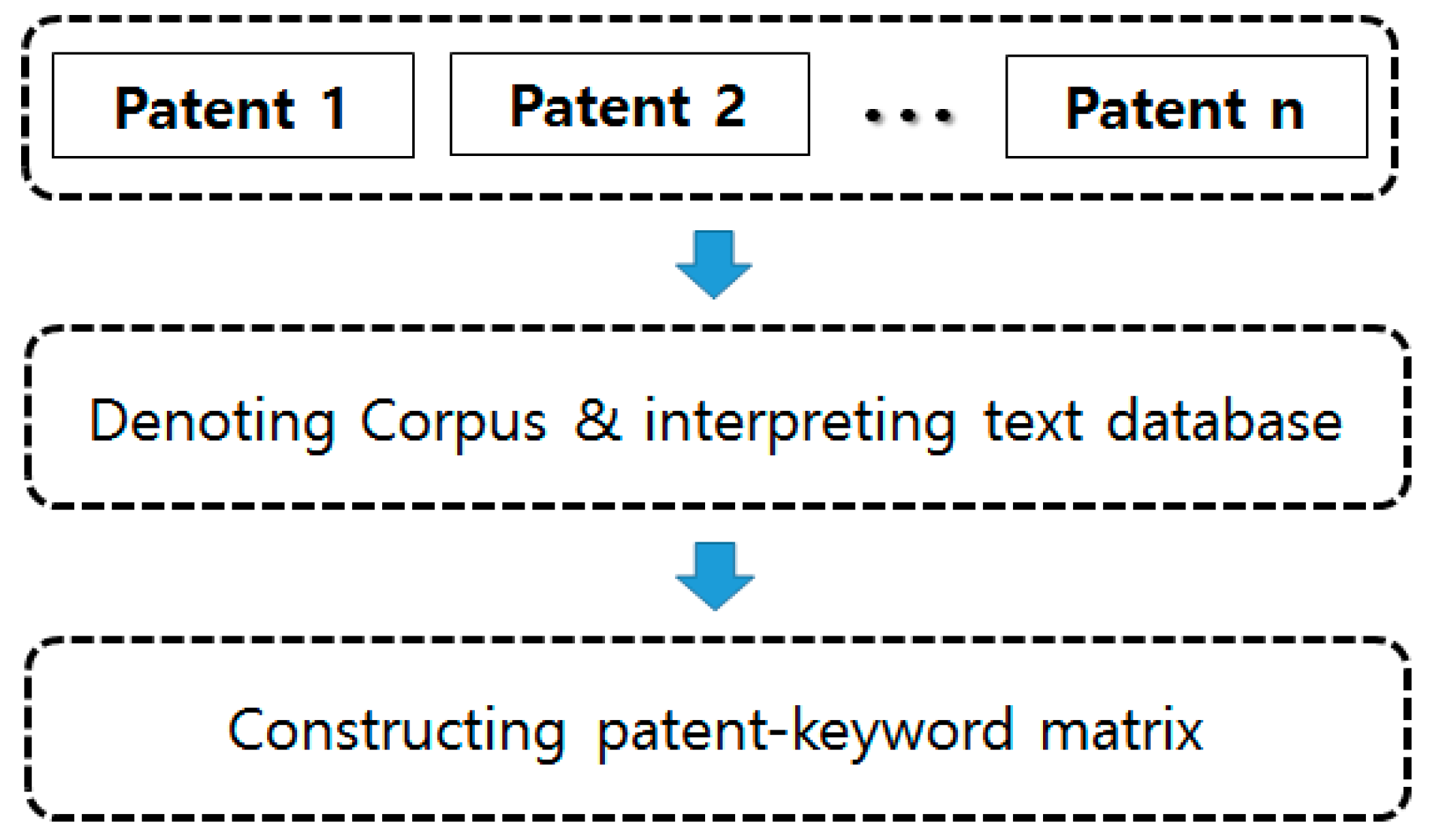
Patent analysis has been a popular research topic in the TF of MOT. Many studies on patent analysis have focused on technology analysis [4,5,22,24,29]. They preprocessed patent documents using text mining techniques to construct the structured data suitable for statistical analysis. Nakamura et al. (2015) studied on a knowledge combining modeling using cluster analysis. Using patent document data, they proposed the depth and breadth combination model for the measurement of knowledge similarity between different technological domains by patent clustering [30]. To construct a strategic road map of robotics technologies for the power industry, Daim et al. (2017) represented a multi-criteria technology assessment using the technology system tree, expert group identification, and co-authorship and related keyword network diagram [31]. Kyebambe et al. (2017) studied the forecasting of emerging technologies using patent analysis. They analyzed the patent citations from patent documents by supervised learning approach [19]. In the retail field, research related to an innovation leading to retail industry growth was carried out by Pantano et al. (2017). The study showed an empirical evidence of the growth from the results of patent analysis [32]. Caviggioli (2016) used the international patent classification (IPC) codes extracted from the patent documents for technology fusion. He analyzed the IPC code data to represent the identification of the drivers of technology convergence [33]. Using text mining techniques and F-term analysis, Song et al. (2017) discovered new technology opportunities. The finding is also based on patent document data [34]. Figure 1 shows the common process of patent analysis.
We retrieve the patent documents related to a target technology from patent databases such as the United States Patent and Trademark Office (USPTO) or WIPS Corporation [35,36]. The USPTO and WIPS are popular patent databases for free and commercial use, respectively. Using preprocessing by text mining techniques, we make a patent–keyword matrix as structured data for statistical analysis, because patent document data are not suitable for statistical analysis [24,25,37,38]. The rows and columns of the matrix represent the patents and keywords, respectively. Additionally, each element of the matrix represents the occurred frequency of a keyword in each patent. This matrix is the same as the table structure of statistical analysis with observation (row) and variable (column). The analytical results of the matrix data are used for the TF. In this paper, we propose a method of interval estimation for statistical analysis of patent technology data. We explain the general methods of interval estimation in the next section.
2.2. Interval Estimation Methods
The estimation and hypothesis tests are the two main parts of statistical inference [39]. Applied statisticians prefer the confidence interval to the hypothesis test, because the interval estimation is more effective than the test in the field. When a frequency value is given, one of the most common statistics is a proportion, p. The Wald confidence interval, based on the asymptotic normality of the maximum likelihood of p, is commonly used [40,41,42]. However, the Wald confidence interval cannot give a confidence interval for p in the case of X = 0 (zero frequency) or the lower bound of the Wald confidence interval with negative value in X ≈ 0, where X is a variable with frequency value. To solve these problems, many researchers have studied other confidence intervals [40,41,42,43,44]. Here, some confidence intervals are introduced for p. First, we show the Wald confidence interval as follows: let X denote the number of successes with a sample size n, and let be a sample proportion. Based on asymptotic normal assumptions [39], the classic confidence interval for the proportion is as follow
where is quantile from a standard normal distribution. Next, we explain the Wilson confidence interval [45].
The terminologies in (2) are the same as the notations of (1). Lastly, the exact confidence interval is based on a binomial distribution; Clopper and Pearson (1934) suggested the exact confidence interval for the true p without approximation [46]. The confidence limits are the solutions in to the following equations, except for the extreme cases of and .
The lower limit is 0 at , and the upper limit is 1 at . Based on the relationship between Binomial and F distribution, the exact confidence interval can be obtained as follows:
where is the quantile of the F distribution with degrees of freedom of a and b. In the context of patent big data, the methods of interval estimation can be an efficient approach to overcome the sparsity of patent data. We, therefore, propose an interval estimation method for the TF in the next section.
3. Interval Estimation for Technology Forecasting
In this paper, we propose a method of interval estimation for the TF. Among the various methods for computing interval estimation, we use the Agresti–Coull confidence interval (which is called an adjusted Wald confidence interval) as follows [43,47,48].
where and . The Agresti–Coull confidence interval is a similar form of Wald confidence interval. Additionally, if z ≈ 2 in the Wilson confidence interval, the center of the Agresti–Coull confidence interval is identical to that of the Wilson confidence interval as follows:
The Agresti–Coull confidence interval is also interpreted as the center of the Wilson’s confidence interval, as a weighted average of and as follows:
Therefore, the point estimator converges to as . They compared actual coverage probabilities with 95% confidence level depending on sample size and the true proportion, and showed much better performance than the Wald and exact confidence intervals. They recommended it for all sample sizes and parameters. Using the adjusted Wald confidence interval, we can control many zero values of the structured data (document–term matrix) that is preprocessed from patent documents. To get patent documents related to target technology, we retrieve patents from patent databases of the world. The most popular databases, USPTO and WIPSON, are used. In the retrieved patent documents related to our target technology, we have to form the structured patent data for our IEM. Figure 2 shows the process of our preprocessing to construct the structured patent data.
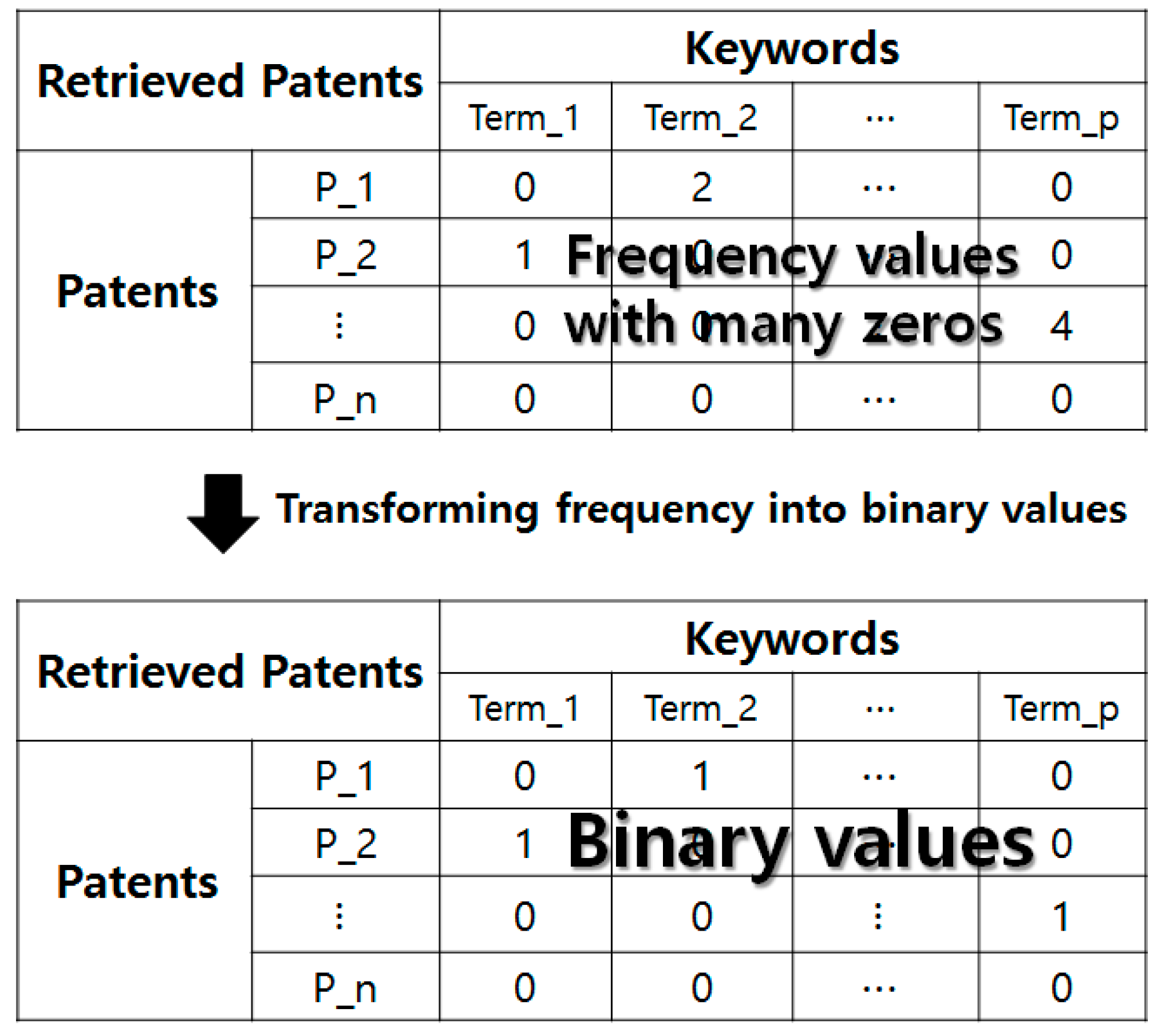
The text document collection based on the retrieved n patent documents is denoted as a corpus, and it is interpreted as a text database. The R data language and its “tm” package are used to construct a patent–keyword matrix from the interpreted text database [37,38,49]. Using the text mining process, we get the structured patent data in top of Figure 3.
The patent–keyword matrix consists of patents and keywords as its rows and columns, respectively. Each element of the matrix is the occurred frequency value of a keyword in a patent. Next, we transform the patent data of frequency values into structured data with binary values for the interval estimation in bottom of Figure 3. In this paper, we use this matrix for our IEM in Apple’s TF. We encounter the sparsity problem in this data structure of Figure 3, because many elements of the matrix are zero values. We have to select a methodology to overcome this problem. In our research, we propose an IEM based on the adjusted Wald confidence interval. Therefore, we perform the IEM from the patent documents related to the target technology according to the following process.
- (Step 1)
- Collecting patent document data
- (1-1)
- Selection of target technology
- (1-2)
- Retrieval of patents related to target technology from patent databases
- (Step 2)
- Constructing structured patent data
- (2-1)
- Collected patent documents imported to R data system
- (2-2)
- Denoting corpus and interpreting text database using patent documents
- (2-3)
- Building patent–keyword matrix with occurred frequency of keyword
- (2-4)
- Changing occurred frequency to binary value
- (Step 3)
- Computing interval estimation of patent keyword
- (3-1)
- Using Agresti–Coull confidence interval for IEM
- (3-2)
- Computing interval estimation of technology keyword for TF
- (Step 4)
- Forecasting future technology
- (4-1)
- Using IEM results of all patent keywords
- (4-2)
- Assigning representative technology to each keyword
- (4-3)
- Predicting future state of target technology
In this paper, we forecast future technologies using the results of our IEM. We compute the estimated intervals of all patent keywords using the IEM. In addition, we can set data related technology to the “data” keyword. The mean (), upper, and lower values of interval estimation provide valuable information to forecast future technology. The larger the values are, the more important the technological keyword is. In statistics, half of the width is called as a margin of error, and the square root part in Equation (5) is called the standard error. Both of them are measures of errors for the interval estimation. The errors are depended on the estimate for p and a sample size, n. With bigger p and less n, the errors are increasing, and the widths are getting wider. It could be interpreted that more errors and wider widths when a bigger p is estimated with smaller sample size. It is quite reasonable. The estimation is not stable with small sample. We should suggest wider interval estimation for better confidence. In the next section, we perform a case study of Apple’s technology.
4. Case Study of Apple Technology
To show how the proposed method can be used to address a real problem, we carried out a case study using Apple’s patent data. Apple has been leading the technological innovation of the global information and communication (ICT) industry [9,10,50,51,52]. Jun and Park (2013) examined the technological innovation of Apple using patent analysis [9]. They analyzed the patent documents of Apple with time series regression, K-means clustering, and social network analysis to understand the technologies of Apple. Additionally, Kim and Jun (2015) studied graphical causal inference and copula regression to analyze the technological keywords of Apple patents [5]. The authors used the technological relationships among Apple’s patent keywords to understand the technological structure of Apple. Previous studies related to Apple’s technologies did not consider technological changes over time and the scope of change in the patent keywords of Apple. We proposed an IEM for building the variable interval of Apple’s keywords over time. We used Apple’s patents issued between 1977 and 2010. We also searched patent data in the patent database of WIPS Corporation [36]. Using text mining techniques including natural language processing [37,38], we made a corpus from searched patent documents and constructed document–term matrix which consists of patent documents (rows) and occurred terms (columns). To select the keywords representing Apple’s technologies, we had help from the domain experts of Apple in the Korea Intellectual Property Strategy Agency (KISTA) [53]. We extracted sixteen major keywords from the collected patent documents related to Apple, as follows: audio, computer, content, data, device, digital, display, image, information, interface, media, memory, network, system, user, and video. To analyze the patent documents of Apple, we formed structured data called patent keyword matrix using text mining techniques. The columns and rows represent patent keywords and years in this matrix, and the elements of the matrix contain the occurred frequency values of keywords by year. Using this data matrix, we computed interval estimations for each keyword. We grouped the sixteen keywords into four technological groups. Like the approach to keyword selection of Apple technology, we got help from the domain experts of Apple in the Korea Intellectual Property Strategy Agency (KISTA) for technological classification of Apple. Table 1 shows the four technological groups of Apple keywords and their representative technologies.
In Table 1, Group 1 consists of four keywords (i.e., “content”, “data”, “information”, and “memory”) and we defined the representative technology of this group as “Data”. In the same way, the representative technologies of Groups 2–4 are “Application”, “System”, and “User Interface”, respectively. The four major technologies are considered to assess Apple’s technological sustainability. We computed the interval estimations of the keywords and keyword groups.
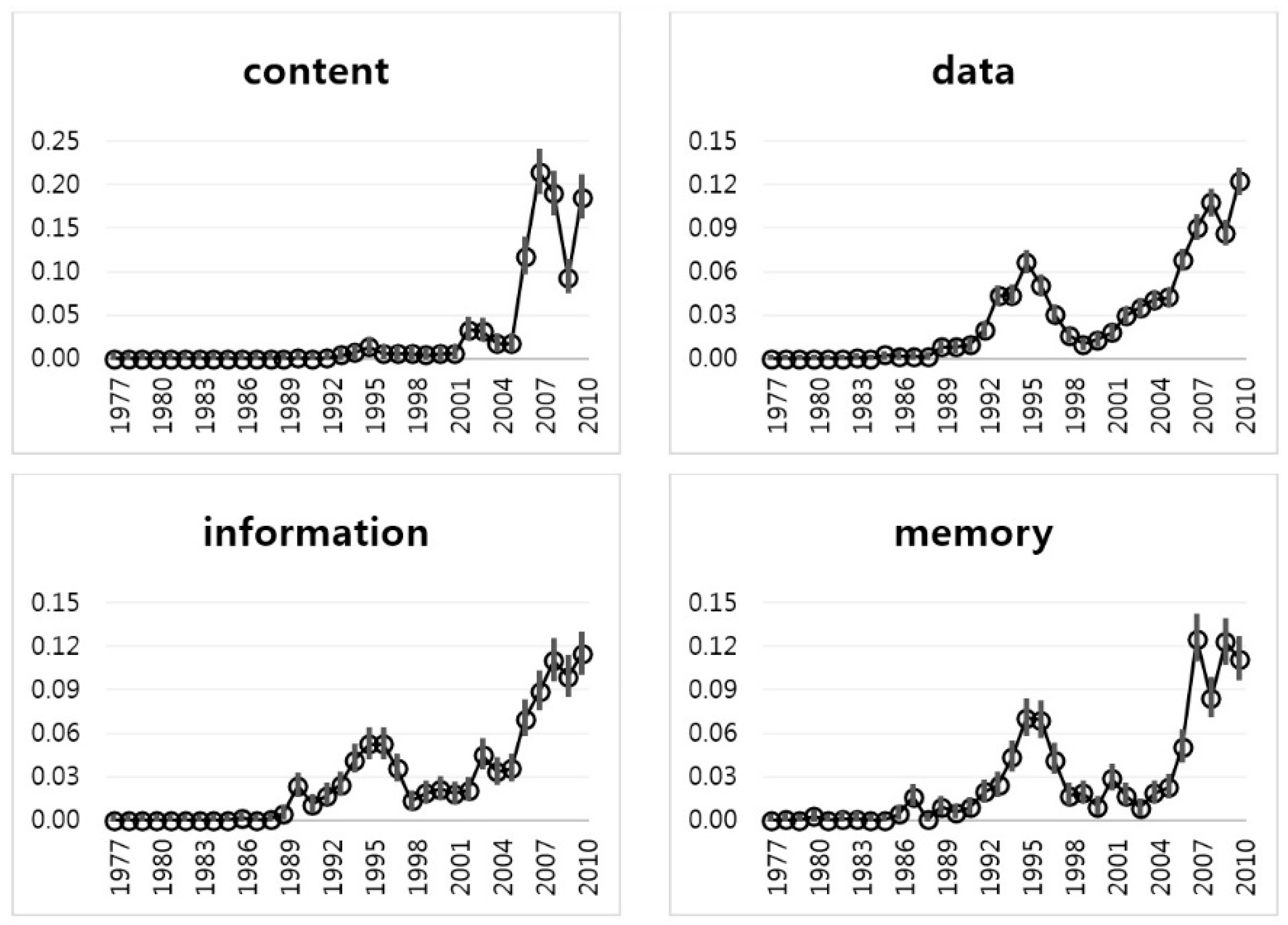
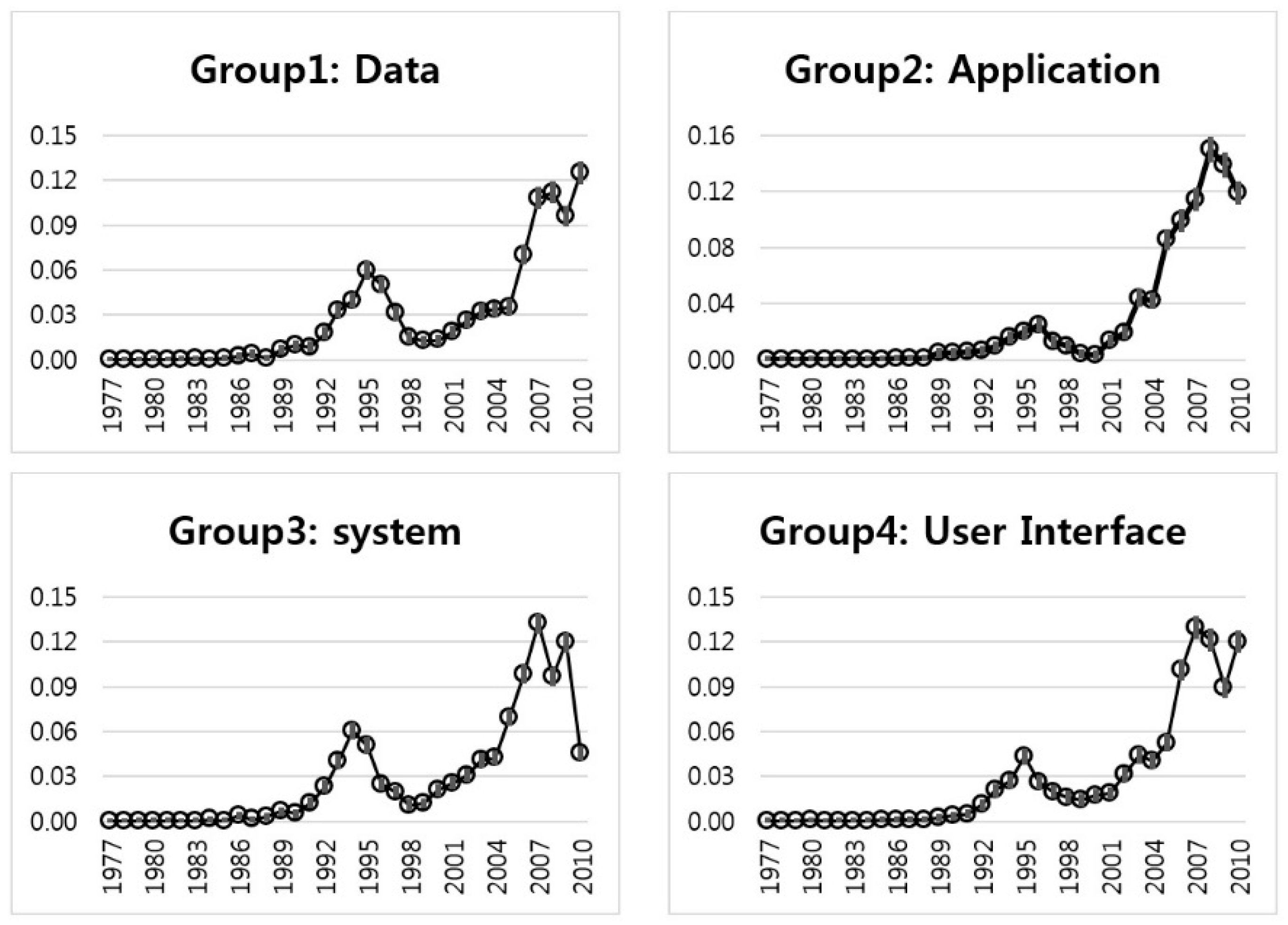
Figure 4 shows the interval estimation plots of four keywords in Group 1. The “content” keyword rose in the late 2000s, dropped in 2009, and then increased again in 2010. The keywords of “data”, “information”, and “memory” were at their peak in 1995. Later, they continued to decrease, but, recently, they have increased rapidly. In the late 1990s, Apple launched a new computer called the iMac. At that time, Apple first turned a profit. We determined that the technology of Group 1 is the sustainable technology of Apple. To discover more detail about the Group 1 technology, we show IEM values, such as the estimate, lower limit, and upper limit of the proportion () IE of each keyword by year in Table 2. Because there was very little frequency before the 1990s, most of the mean values of the keywords were close to zero.
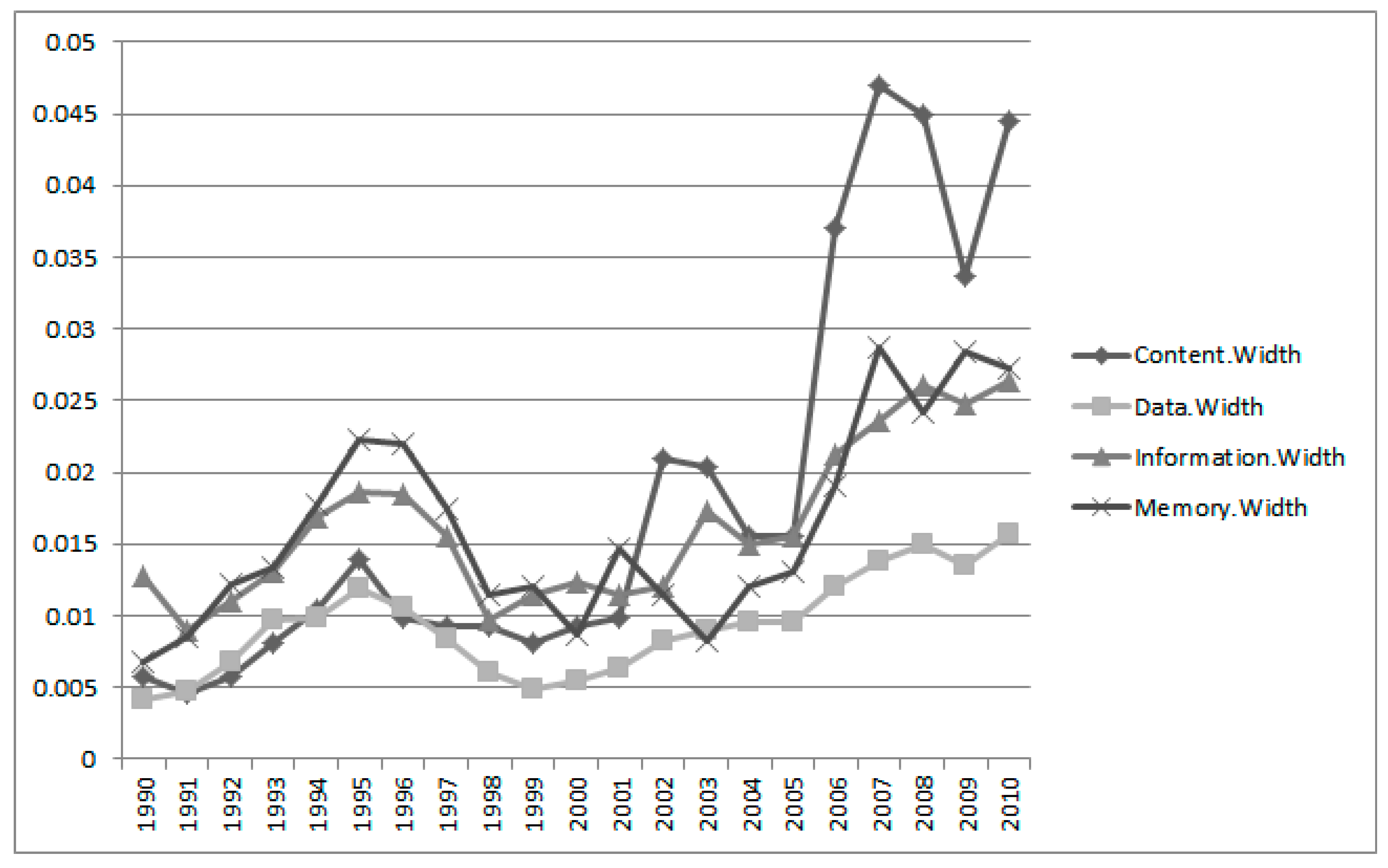
In Figure 5 we extracted meaningful interval estimations results since 1990 from Table 2 to determine the variability of the keywords over time. The interval estimation widths of the keywords of Group 1 were computed from the absolute difference between the upper and lower limits. The width value of the keyword “data” is the smallest one in Group 1. This means that the technology based on data does not fluctuate over time within the Apple technology. In a relative sense, the width value of the keyword “content” fluctuates more than other keywords in Group 1.
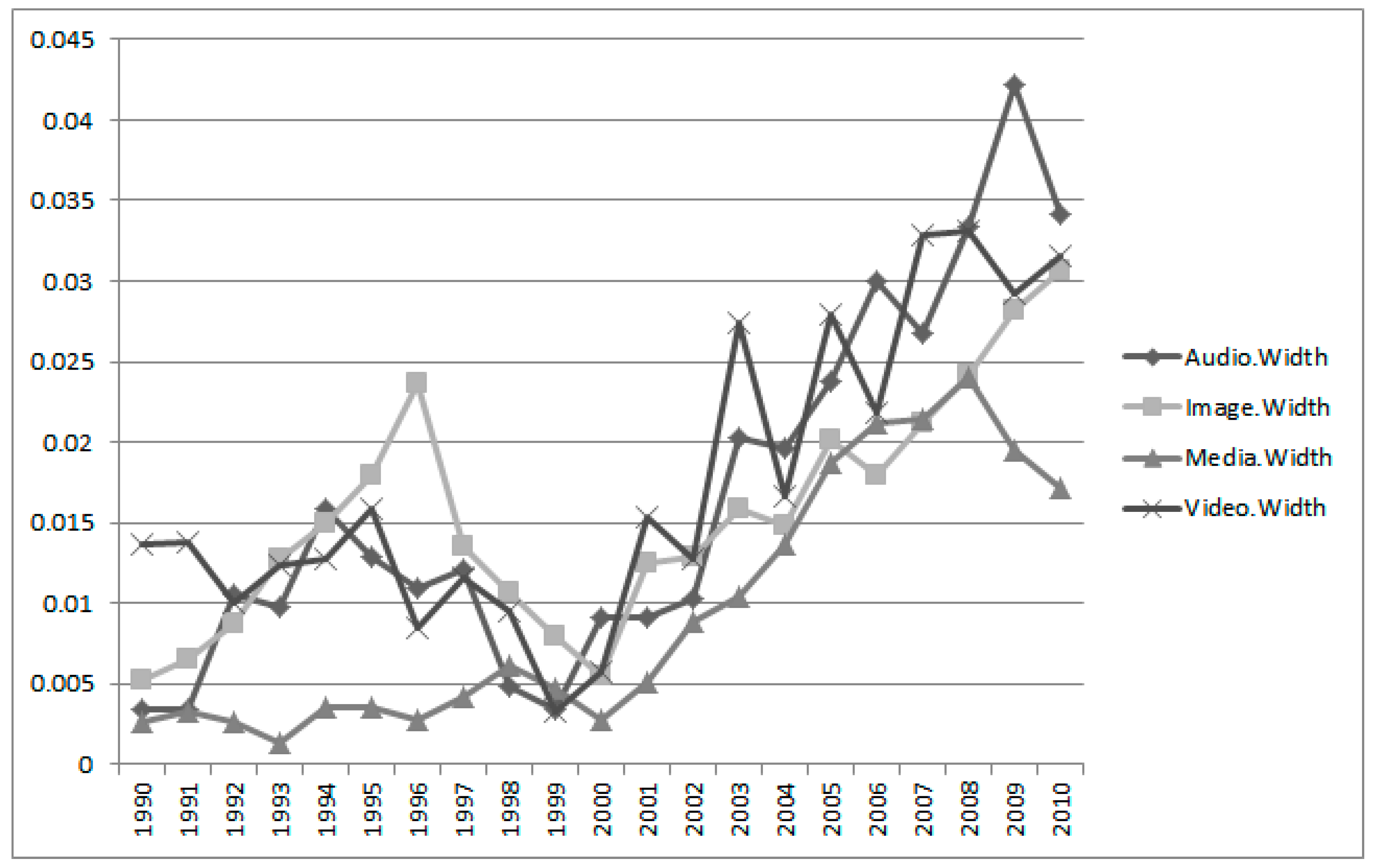
Next, Figure 6 shows the IE plots for Group 2 (i.e., “Application”) with keywords “audio”, “image”, “media”, and “video”. The time trends of most Group 2 keywords differ from the keywords of Group 1. They have no peaks in the late 1990s, except for the keyword of “image”. The keyword “audio” has a peak in 2009. This means that the “audio” technology of Apple was researched and developed relatively recently. The “media” technology is similar to the technology based on “audio”. However, the technology of “video” has fluctuated since the 2000s. Table 3 shows the detailed IEM results of Group 2.
Using the estimate, lower, and upper values, we constructed the interval estimation widths of the keywords of Group 2 in Figure 7. Unlike the visualization result of Group 1, they show large fluctuations. In particular, by the year 2000 the range of fluctuations was larger than before. We concluded, therefore, that the technology of “Data” (Group 1) is more stable than the “Application” technology (Group 2).
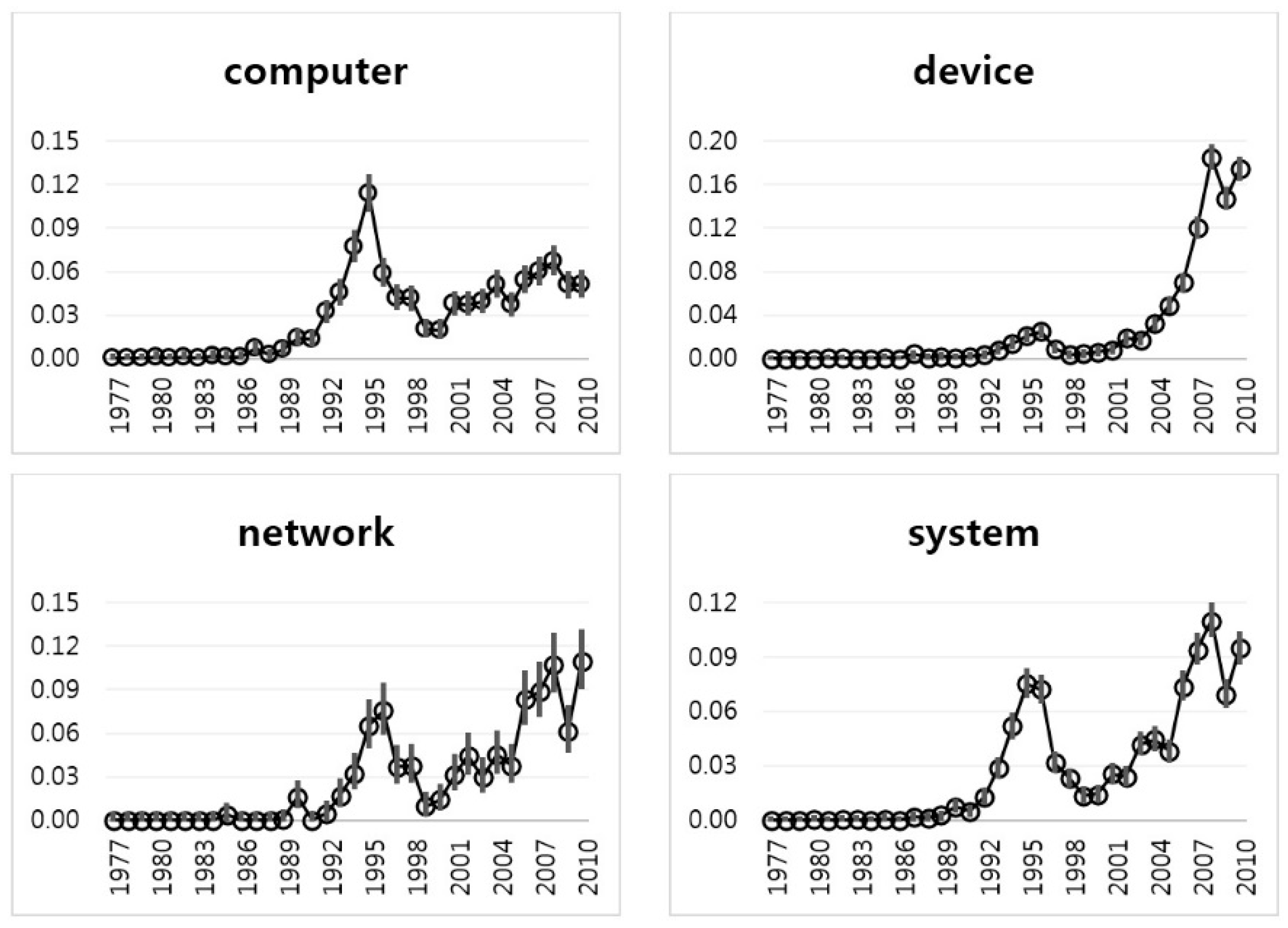
Figure 8 shows the IE plots of Group 3 with the keywords of “computer”, “device”, “network”, and “system”. The trends of “computer”, “network”, and “system” are similar to those of the keywords of Group 1. They have peaks in 1995. The keyword of “device”, however, has a peak in 2007. This is more recent than other keywords in Group 3. We show more detailed IEM results of Group 3 keywords in Table 4. We found that the sparsity of Group 3 is less than that of Group 1 or Group 2, because most mean values of Group 3 keywords are not zero. This means that the technology of Group 3 (System technology) is very active in the Apple Company.
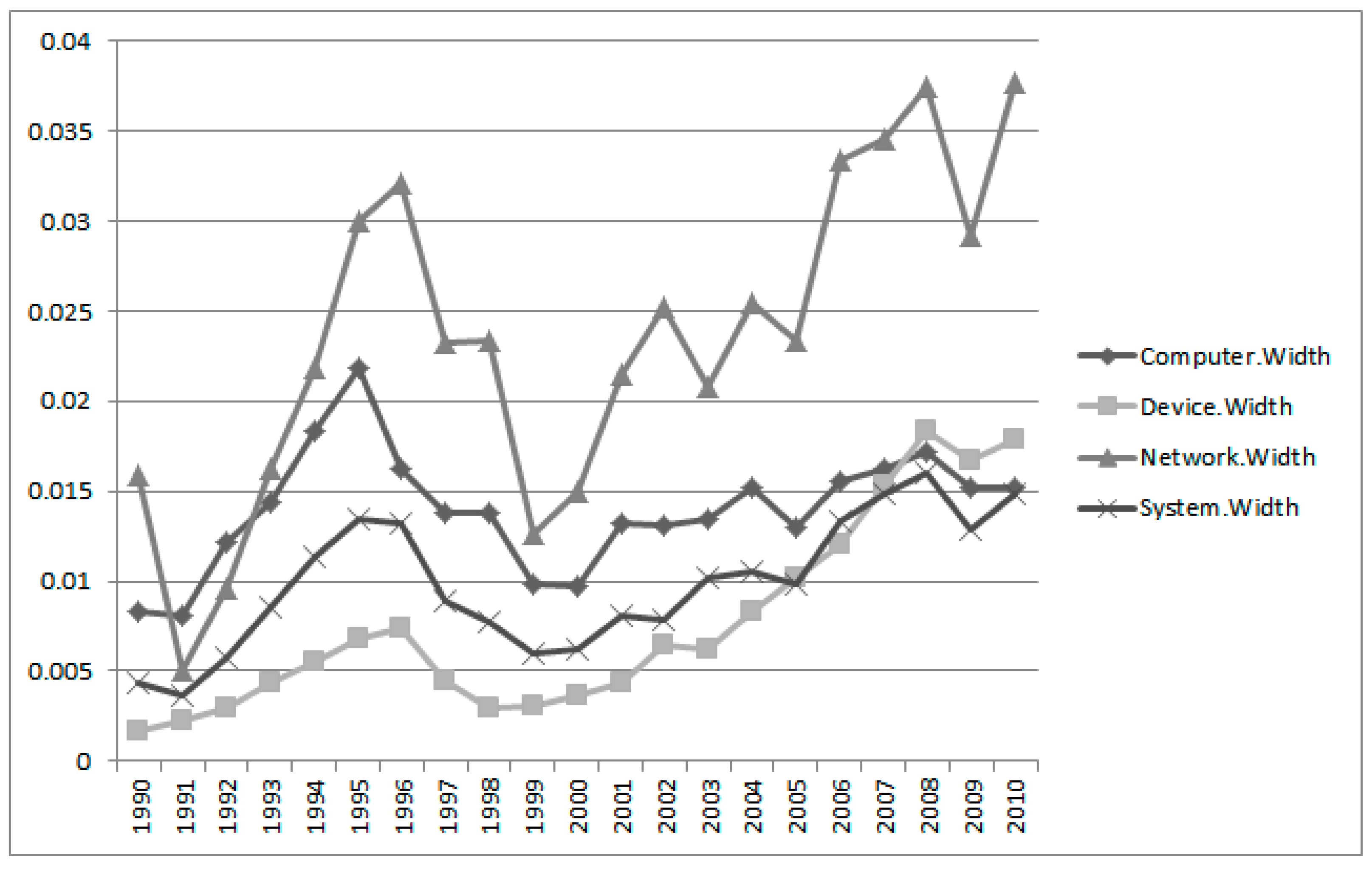
In Figure 9, we calculated the visualization of interval estimation widths of Group 3 using the results of Table 4. The results show that the variations of Group 3 keywords are stable except for “network”. We conclude, therefore, that the technology based on Group 3 is sustainable in the Apple Company.
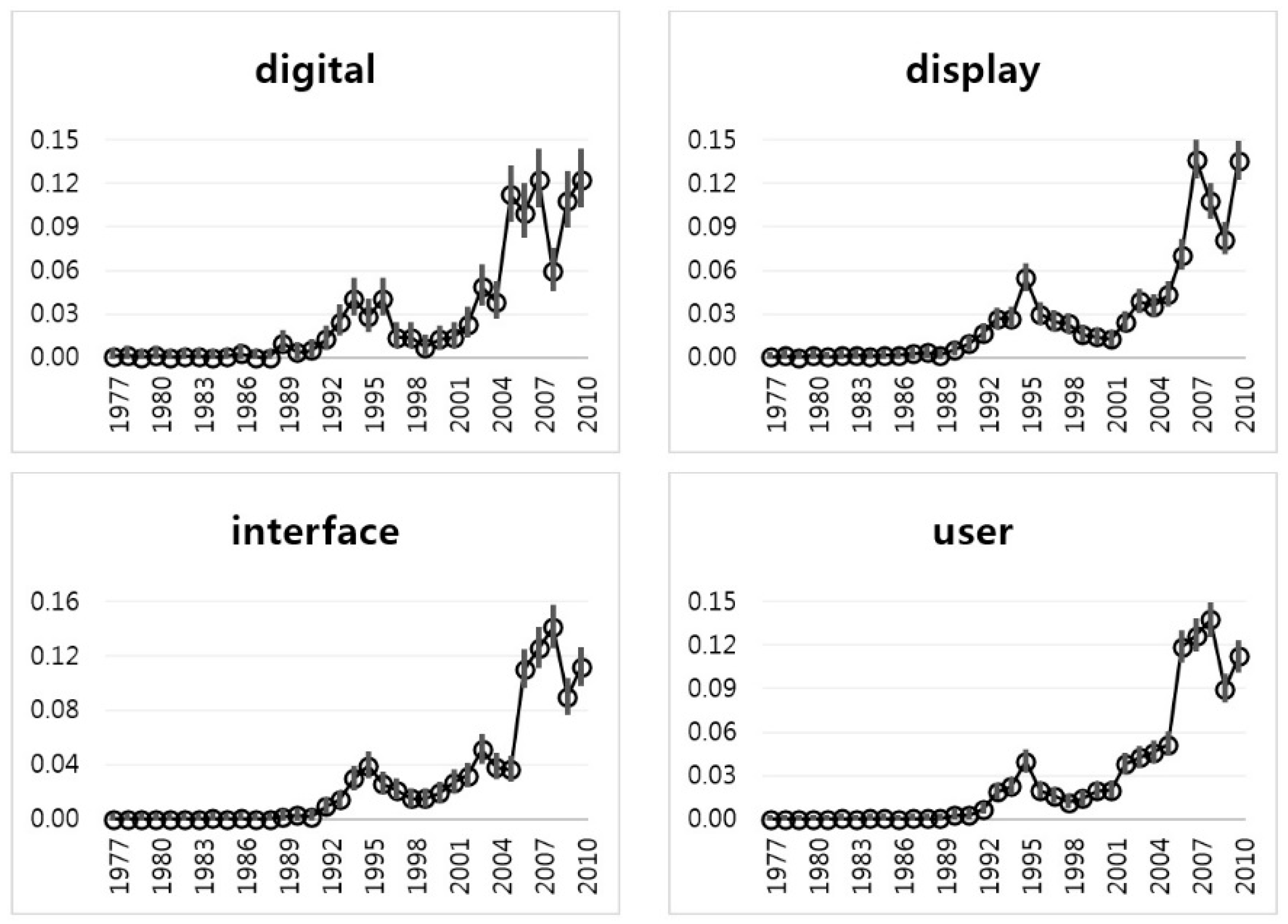
Next, Figure 10 represents the interval estimation plots of Group 4. The technological trends of Group 4 keywords are similar to the trend of Group 1. The relative height of Group 4, however, is lower than that of Group 1. We see that the technology of Group 4 (User Interface technology) is collaborative with the technology of Group 1 (Data technology). This means that Apple has developed the technologies of user interface and data together. Table 5 expresses the interval estimation results of the keywords in Group 4. Like the results of Group 3, the sparseness of Group 4 has relaxed somewhat. We see that the mean values of the keywords in Group 4 increase steadily.
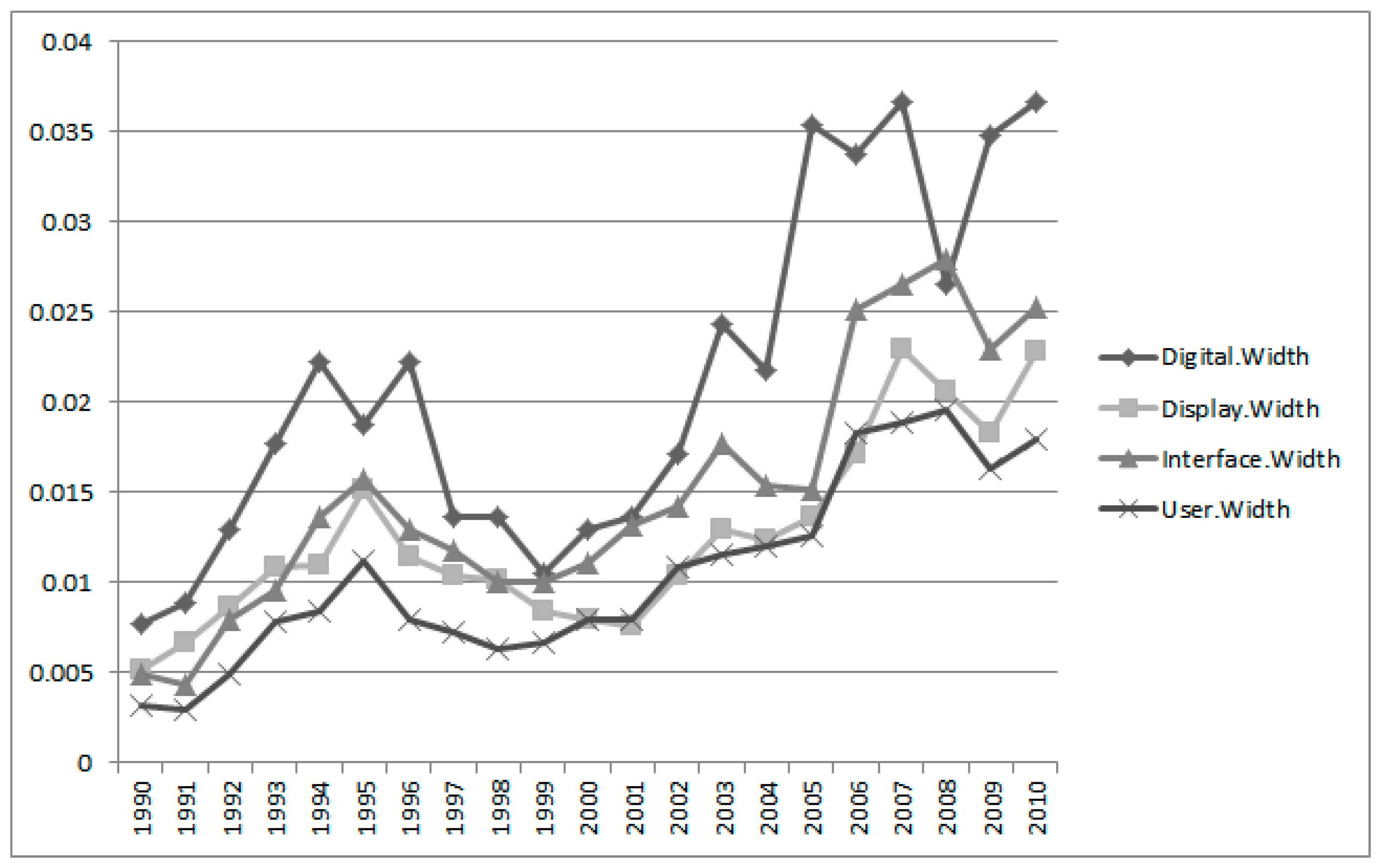
Figure 11 shows interval estimation widths of Group 4 keywords. The fluctuation of the “digital” keyword is larger than other keywords of Group 4.
Until now, we explained the IEM results according to technological groups. Finally, we carried out the IEM for all integrated groups. Figure 12 shows the interval estimation plots of all groups. The technologies of Groups 1, 3, and 4 have their peaks in 1995. However, the Group 2 technology has its peak in 2007. We see that the Apple Company has recently been focusing on technology based on application. Table 6 shows the interval estimation results of all groups.
Using the results of Table 6, we computed the interval estimation widths of all groups in Figure 13.
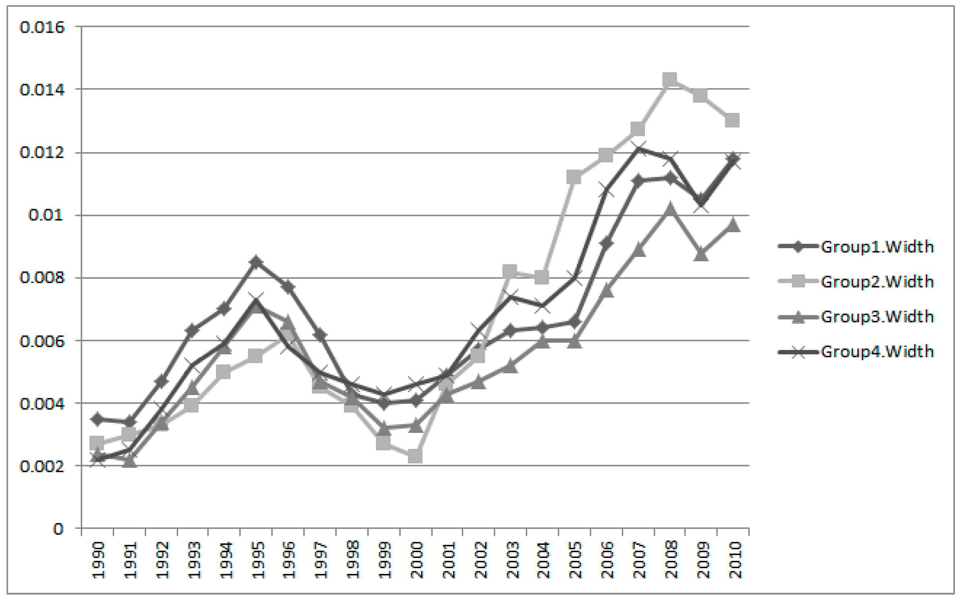
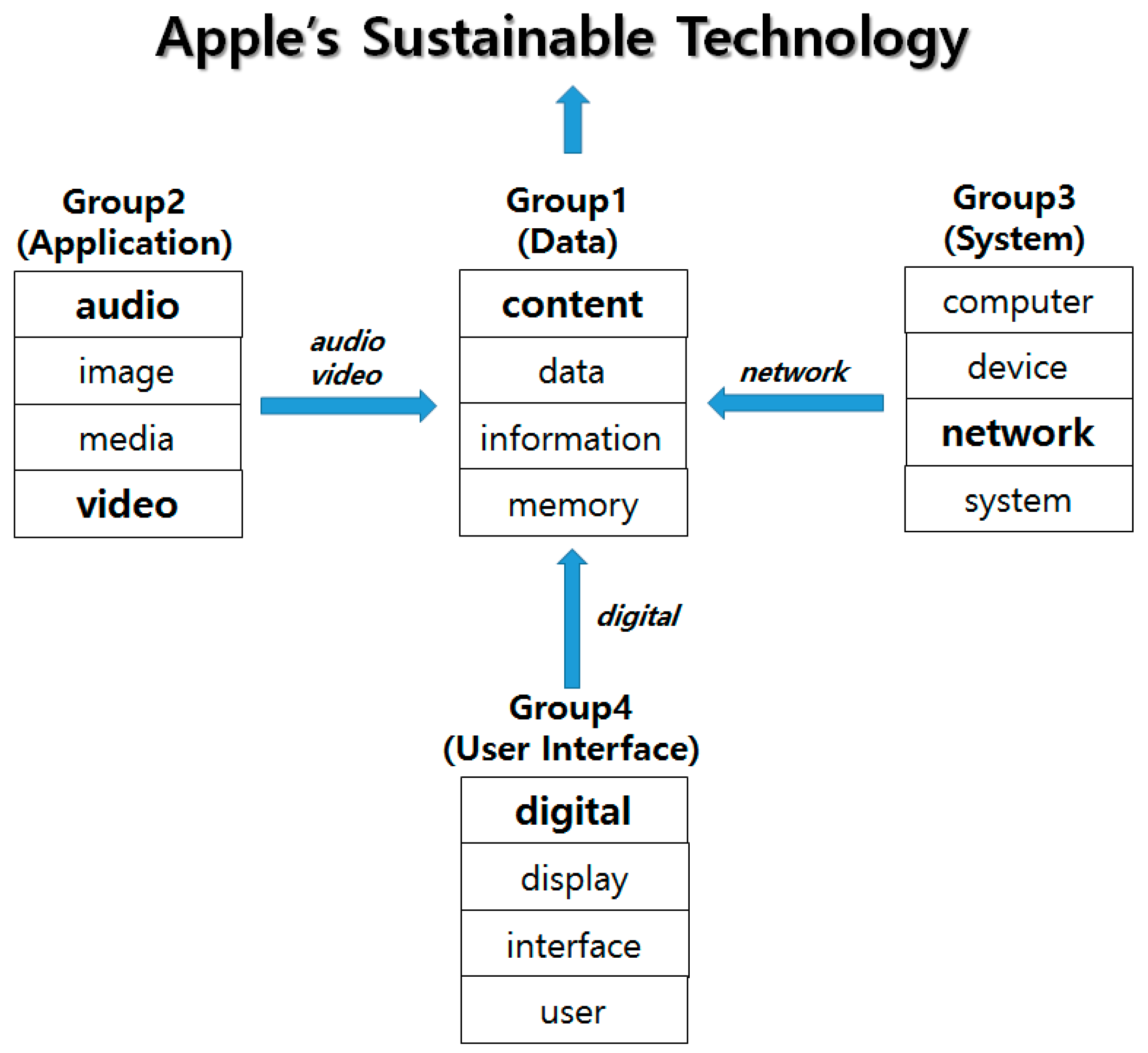
We see that the fluctuation patterns of all groups are similar. In 1995, the peaks of all fluctuations were visible, and recently fluctuations have increased. From the IEM results of all keywords and groups, we obtained the technological structure for Apple’s sustainability in Figure 14.
Group 1 consists of four keywords (i.e., “content”, “data”, “information”, and “memory”). Using the four keywords, we defined the representative technology of Group 1 as data-based technology. Among these keywords, the “content” keyword has the most influence on the Group 1 technology. In Figure 14, we expressed the keyword in bold. The same interpretations used for Group 1 apply to the other groups in Figure 14. The technology of Group 2 is influenced by the technologies based on “audio”, “image”, “media”, and “video”. The technologies of “audio” and “video” dominate the Group 2 technology. Among the four keywords included in Group 3, the “network” keyword has the most influence on the system-based technology of Group 3. Therefore, the technologies of Groups 2–4 affect the technology of Group 1. Apple possesses technologies related to application, system, and user interface, and they have become the basis for developing the data technology. Consequently, this technology structure drives the sustainable technology of Apple. In general analysis without sparsity problem, the frequency values are better data than the binary data. The sparsity problem causes analytical difficulties in patent data analysis. Thus, diverse studies were performed to overcome the problem. In this paper, we also tried to solve the problem by proposed interval estimation method using binary values, and we showed the validity of our method.
5. Discussion
Recently, technology analysis has relied on patent analysis by objective and quantitative statistical models rather than Delphi survey that is based on expert subjective knowledge. Thus, many studies related to patent data analysis have been performed in diverse fields. In order to use statistical models for patent data, we first have to convert the retrieved patent documents into a formal data structure. The structured patent data is a matrix consisting of patent keywords and their frequency values. Each row and column of the matrix represent a patent and a technological keyword, respectively. An element of the matrix is the frequency value of each keyword occurred in a patent document. In general, this matrix is very sparse, that is, most elements have a value of zero. Therefore, most of studies on patent analysis tried to solve the sparsity problem, and carried out statistical modeling or machine learning algorithm for technology analysis. TF is also an attractive field in technology analysis. Because companies want to know the future state of technology in order to increase their market competitiveness. The traditional TF studies mainly consisted of regression analysis that confirms the relation between technologies, time series analysis that analyzes the trend of technology over time, or cluster analysis that groups similar technologies. In the studies, each TF model was independently developed and used. However, our IEM-based TF method is a technology analysis that considered the technological trends of patent keywords over time and technological relations between patent keywords simultaneously. In particular, the TF results are expressed in the form of interval instead of single predictive value, reflecting both the diversity of prediction and uncertainty. In addition, we divided Apple’s technologies into four sub technology groups, and estimated the confidence intervals of occurred frequencies of technological keywords included in four groups. From the results of our proposed method, we can find the future trends of technological keywords of Apple’s technology, and predict Apple's future product development through a combination of the keywords with similar trends. We can apply the proposed method not only to Apple but also to other companies' technology analysis, so that we can predict product development as well as understand the technology possessed by the company. Our research does not provide a specific R&D plan for TF. If we want to a build detailed plan for technology development, we need help from the experts in the relevant field of technology. Future research needs to consider a methodology that can provide more specific R&D plan.
6. Conclusions
We proposed a statistical method of patent keyword analysis for TF. We used an interval estimation to make the proposed IEM. In addition, we applied text mining techniques to construct structured patent data suitable for statistical analysis using the R data language and its “tm” package. The structured data consisted of a patent–keyword matrix with occurred frequencies of all selected keywords, and we converted the frequency values to binary data for the IEM. From the results of IEM, we obtained the mean and confidence interval for each keyword. We assigned a representative technology to each keyword, and forecasted the future of the given technology. In this paper, we applied our IEM to Apple’s technology. We found that Apple’s product technology is based on four technological groups. They are data, application, system, and user interface technologies. In addition, the data technology is core and is a sustainable technology necessary for future development. The other technologies (i.e., application, system, and user interface) affect the development of the data technology. We used patents in 34 years between 1977 and 2010. However, in early years, there were few patents with 0 frequency. Only from 1990 some patents could be selected. Using only patents in the most current 20 years, we tried to forecast technology, and they are also only Apple’s patents. However, when we want to apply in general, they are not enough to forecast technology. To generalize the outputs, we should use interval estimation. We could use 95% interval estimation to forecast technology with 95% confidence in general.
This research contributes to an understanding of technological relationships, R&D planning, and new product development in a company. Our research has a limitation because we only used one interval estimation, though the estimation is superior to other interval estimations. In addition, we provided the technological structure for Apple’s sustainable technology by the results of our interval estimation. This does not show directly the future technology of Apple, but the domain experts of Apple technology can perform technology forecasting using the results of our case study of Apple. Thus, the final implication of this paper is depended upon the roles of domain experts. In our future work, we will study the integrated method of diverse interval estimations for TF. This connects the result of interval estimation to TF directly without the efforts of domain experts.
Acknowledgments
This research was supported by Basic Science Research Program through the National Research Foundation of Korea (NRF) funded by the Ministry of Education (NRF-2017R1D1A3B03031152).
Author Contributions
Daiho Uhm and Jea-Bok Ryu designed this research and collected the dataset for the experiment. Sunghae Jun analyzed the data to show the validity of this paper and wrote the paper and performed all the research steps. In addition, all authors have cooperated with each other for revising the paper.
Conflicts of Interest
The authors declare no conflict of interest.
References
- Ittipanuvat, V.; Fujita, K.; Sakata, I.; Kajikawa, Y. Finding linkage between technology and social issue: A Literature Based Discovery approach. J. Eng. Technol. Manag. 2014, 32, 160–184. [Google Scholar] [CrossRef]
- Roper, A.T.; Cunningham, S.W.; Porter, A.L.; Mason, T.W.; Rossini, F.A.; Banks, J. Forecasting and Management of Technology; John Wiley & Sons: New York, NY, USA, 2011. [Google Scholar]
- Choi, S.; Jun, S. Vacant technology forecasting using new Bayesian patent clustering. Technol. Anal. Strateg. Manag. 2014, 26, 241–251. [Google Scholar] [CrossRef]
- Jun, S.; Park, S.; Jang, D. Technology Forecasting using Matrix Map and Patent Clustering. Ind. Manag. Data Syst. 2012, 112, 786–807. [Google Scholar] [CrossRef]
- Kim, J.M.; Jun, S. Graphical Causal Inference and Copula Regression Model for Apple Keywords by Text Mining. Adv. Eng. Inform. 2015, 29, 918–929. [Google Scholar] [CrossRef]
- Choi, J.; Hwang, Y.S. Patent keyword network analysis for improving technology development efficiency. Technol. Forecast. Soc. Chang. 2014, 83, 170–182. [Google Scholar] [CrossRef]
- Huang, L.; Zhang, Y.; Guo, Y.; Zhu, D.; Porter, A.L. Four dimensional Science and Technology planning: A new approach based on bibliometrics and technology roadmapping. Technol. Forecast. Soc. Chang. 2014, 81, 39–48. [Google Scholar] [CrossRef]
- Jin, G.; Jeong, Y.; Yoon, B. Technology-driven roadmaps for identifying new product/market opportunities: Use of text mining and quality function deployment. Adv. Eng. Inform. 2015, 29, 126–138. [Google Scholar] [CrossRef]
- Jun, S.; Park, S. Examining technological innovation of Apple using patent analysis. Ind. Manag. Data Syst. 2013, 113, 890–907. [Google Scholar] [CrossRef]
- Keller, J.; Gracht, H.A.V.D. The influence of information and communication technology (ICT) on future foresight processes—Results from a Delphi survey. Technol. Forecast. Soc. Chang. 2014, 85, 81–92. [Google Scholar] [CrossRef]
- Trappey, C.V.; Wu, H.; Taghaboni-Dutta, F.; Trappey, A.J.C. Using patent data for technology forecasting: China RFID patent analysis. Adv. Eng. Inform. 2011, 25, 53–64. [Google Scholar] [CrossRef]
- Trappey, C.V.; Trappey, A.J.C.; Peng, H.; Lin, L.; Wang, T. A knowledge centric methodology for dental implant technology assessment using ontology based patent analysis and clinical meta-analysis. Adv. Eng. Inform. 2014, 28, 153–165. [Google Scholar] [CrossRef]
- Hanke, J.E.; Wichern, D. Business Forecasting, 9th ed.; Pearson: Essex, UK, 2014. [Google Scholar]
- Glahn, H.R.; Lowry, D.A. The Use of Model Output Statistics (MOS) in Objective Weather Forecasting. J. Appl. Meteorol. 1972, 11, 1203–1211. [Google Scholar] [CrossRef]
- Bowerman, B.L.; O’Connell, R.T.; Koehler, A.B. Forecasting, Time Series, and Regression, an Applied Approach; Brooks/Cole: Independence, KY, USA, 2005. [Google Scholar]
- Zhang, G.P. Neural Networks in Business Forecasting; IBM Press: Hershey, PA, USA, 2004. [Google Scholar]
- Spann, M.; Skiera, B. Internet-Based Virtual Stock Markets for Business Forecasting. Manag. Sci. 2003, 49, 1310–1326. [Google Scholar] [CrossRef]
- Mathur, S.; Kumar, A.; Chandra, M. A Feature Based Neural Network Model for Weather Forecasting. Int. J. Comput. Intell. 2008, 4, 209–216. [Google Scholar]
- Kyebambe, M.N.; Cheng, G.; Huang, Y.; He, C.; Zhang, Z. Forecasting emerging technologies: A supervised learning approach through patent analysis. Technol. Forecast. Soc. Chang. 2017, 125, 236–244. [Google Scholar] [CrossRef]
- OuYang, K.; Weng, C.S. A New Comprehensive Patent Analysis Approach for New Product Design in Mechanical Engineering. Technol. Forecast. Soc. Chang. 2011, 78, 1183–1199. [Google Scholar] [CrossRef]
- Trappey, A.J.C.; Trappey, C.V.; Wu, C.; Lin, C. A patent quality analysis for innovative technology and product development. Adv. Eng. Inform. 2012, 26, 26–34. [Google Scholar] [CrossRef]
- Park, S.; Kim, J.; Lee, H.; Jang, D.; Jun, S. Methodology of technological evolution for three-dimensional printing. Ind. Manag. Data Syst. 2016, 116, 122–146. [Google Scholar] [CrossRef]
- Tseng, Y.; Juang, D.; Wang, Y.; Lin, C. Text mining for patent map analysis. In Proceedings of the IACIS Pacific Conference, Taipei, Taiwan, 19–21 May 2005; pp. 1109–1116. [Google Scholar]
- Tseng, Y.; Lin, C.; Lin, Y. Text mining techniques for patent analysis. Inf. Process. Manag. 2007, 43, 1216–1247. [Google Scholar] [CrossRef]
- Jun, S.; Park, S.; Jang, D. Document Clustering Method Using Dimension Reduction and Support Vector Clustering to Overcome Sparseness. Expert Syst. Appl. 2014, 41, 3204–3212. [Google Scholar] [CrossRef]
- Choi, J.; Jun, S.; Park, S. A Patent Analysis for Sustainable Technology Management. Sustainability 2016, 8, 688. [Google Scholar] [CrossRef]
- Park, S.; Lee, S.; Jun, S. A Network Analysis Model for Selecting Sustainable Technology. Sustainability 2015, 7, 13126–13141. [Google Scholar] [CrossRef]
- Park, S.; Jun, S. Statistical Technology Analysis for Competitive Sustainability of Three Dimensional Printing. Sustainability 2017, 9, 1142. [Google Scholar] [CrossRef]
- Trappey, A.J.; Trappey, C.V. An R&D knowledge management method for patent document summarization. Ind. Manag. Data Syst. 2008, 108, 245–257. [Google Scholar]
- Nakamura, H.; Suzuki, S.; Sakata, I.; Kajikawa, Y. Knowledge combination modeling: The measurement of knowledge similarity between different technological domains. Technol. Forecast. Soc. Chang. 2015, 94, 187–201. [Google Scholar] [CrossRef]
- Daim, T.U.; Yoon, B.-S.; Lindenberg, J.; Grizzi, R.; Estep, J.; Oliver, T. Strategic roadmapping of robotics technologies for the power industry: A multicriteria technology assessment. Technol. Forecast. Soc. Chang. 2017. [Google Scholar] [CrossRef]
- Pantano, E.; Priporas, C.-V.; Sorace, S.; Iazzolino, G. Does innovation-orientation lead to retail industry growth? Empirical evidence from patent analysis. J. Retail. Consum. Serv. 2017, 34, 88–94. [Google Scholar] [CrossRef]
- Caviggioli, F. Technology fusion: Identification and analysis of the drivers of technology convergence using patent data. Technovation 2016, 55–56, 22–32. [Google Scholar] [CrossRef]
- Song, K.; Kim, K.S.; Lee, S. Discovering new technology opportunities based on patents: Text-mining and F-term analysis. Technovation 2017, 60–61, 1–14. [Google Scholar] [CrossRef]
- The United States Patent and Trademark Office (USPTO). Available online: http://www.uspto.gov/ (accessed on 1 March 2016).
- Wips on coporation, WIPS Corporation. Available online: http://www.wipson.com/ (accessed on 15 May 2016).
- Feinerer, I.; Hornik, K.; Meyer, D. Text mining infrastructure in R. J. Stat. Softw. 2008, 25, 1–54. [Google Scholar] [CrossRef]
- Feinerer, I.; Hornik, K. Text Mining Package-Package tm. In CRAN R-Project; CRAN R-Project: Vienna, Austria, 2017. [Google Scholar]
- Akritas, M. Probability and Statistics with R; Pearson: New York, NY, USA, 2015. [Google Scholar]
- Brown, L.D.; Cai, T.T.; DasGupta, A. Interval estimation for a binomial proportion (with discussion). Stat. Sci. 2001, 16, 101–133. [Google Scholar]
- Newcombe, R.G. Two-sided confidence intervals for the single proportion: Comparison of seven methods. Stat. Med. 1998, 17, 857–872. [Google Scholar] [CrossRef]
- Ryu, J.B. A short consideration of binomial confidence interval. Commun. Korean Stat. Soc. 2009, 16, 731–743. [Google Scholar] [CrossRef]
- Agresti, A.; Coull, B.A. Approximate is better than “Exact” for interval estimation of Binomial proportions. Am. Stat. 1998, 52, 119–126. [Google Scholar]
- Vollset, S.E. Confidence intervals for a binomial proportion. Stat. Med. 1993, 12, 809–824. [Google Scholar] [CrossRef] [PubMed]
- Wilson, E.B. Probable inference, the law of succession, and statistical inference. J. Am. Stat. Assoc. 1927, 22, 209–212. [Google Scholar] [CrossRef]
- Clopper, C.J.; Pearson, E.S. The use of confidence or fiducial limits illustrated in the case of the Binomial. Biometrika 1934, 26, 404–413. [Google Scholar] [CrossRef]
- Bonett, D.G.; Price, R.M. Adjusted Wald confidence interval for a difference of binomial proportions based on paired data. J. Educ. Behav. Stat. 2012, 37, 479–488. [Google Scholar] [CrossRef]
- Wu, H.; Neale, M.C. Adjusted confidence intervals for a bounded parameter. Behav. Genet. 2012, 42, 886–898. [Google Scholar] [CrossRef] [PubMed]
- R Development Core Team. R: A Language and Environment for Statistical Computing; R Foundation for Statistical Computing: Vienna, Austria, 2017. [Google Scholar]
- Hung, C.Y.; Lee, W.Y.; Wang, D.S. Strategic foresight using a modified Delphi with end-user participation: A case study of the iPad’s impact on Taiwan’s PC ecosystem. Technol. Forecast. Soc. Chang. 2013, 80, 485–497. [Google Scholar] [CrossRef]
- Linden, G.; Kraemer, K.L.; Dedrick, J. Who captures value in a global innovation network?: The case of Apple’s iPod. Commun. ACM-Being Hum. Digit. Age 2009, 52, 140–144. [Google Scholar] [CrossRef]
- Pontiskoski, E.; Asakawa, K. Overcoming Barriers to Open Innovation at Apple, Nintendo and Nokia. World Acad. Sci. Eng. Technol. 2009, 53, 372–377. [Google Scholar]
- Korea Intellectual Property Strategy Agency (KISTA). Available online: http://www.kista.or.kr (accessed on 1 July 2017).
Figure 1.
Patent analysis process.

Figure 2.
Text mining process for structured patent data.

Figure 3.
Structured patent data.

Figure 4.
Interval estimation plots of Group 1: content, data, information, and memory.

Figure 5.
IE widths of Group 1 keywords.

Figure 6.
Interval estimation plots of Group 2: audio, image, media, and video.

Figure 7.
IE widths of Group 2 keywords.

Figure 8.
Interval estimation plots of Group 3: computer, device, network, and system.

Figure 9.
IE widths of Group 3 keywords.

Figure 10.
Interval estimation plots of Group 4: digital, display, interface, and user.

Figure 11.
IE widths of Group 4 keywords.

Figure 12.
Interval estimation plots of all groups.

Figure 13.
IE widths of all groups’ keywords.

Figure 14.
Technological structure for Apple’s sustainable technology.


Table 1.
Four technology groups of Apple keywords.
| Group | Group 1 | Group 2 | Group 3 | Group 4 |
|---|---|---|---|---|
| Keyword | content | audio | computer | digital |
| data | image | device | display | |
| information | media | network | interface | |
| memory | video | system | user | |
| Representative Technology | Data | Application | System | User Interface |
Table 2.
Interval estimation of Group 1: content, data, information, and memory.
| Years | Content | Data | Information | Memory | ||||||||
|---|---|---|---|---|---|---|---|---|---|---|---|---|
| Lower | Upper | Lower | Upper | Lower | Upper | Lower | Upper | |||||
| 1977 | −0.0007 | 0.0000 | 0.0039 | −0.0001 | 0.0000 | 0.0007 | −0.0004 | 0.0000 | 0.0021 | −0.0004 | 0.0000 | 0.0022 |
| 1978 | −0.0007 | 0.0000 | 0.0039 | −0.0001 | 0.0000 | 0.0007 | −0.0004 | 0.0000 | 0.0021 | −0.0002 | 0.0005 | 0.0030 |
| 1979 | −0.0007 | 0.0000 | 0.0039 | −0.0001 | 0.0000 | 0.0007 | −0.0004 | 0.0000 | 0.0021 | −0.0004 | 0.0000 | 0.0022 |
| 1980 | −0.0007 | 0.0000 | 0.0039 | −0.0001 | 0.0001 | 0.0009 | −0.0004 | 0.0000 | 0.0021 | 0.0009 | 0.0024 | 0.0059 |
| 1981 | −0.0007 | 0.0000 | 0.0039 | −0.0001 | 0.0001 | 0.0009 | −0.0004 | 0.0000 | 0.0021 | −0.0004 | 0.0000 | 0.0022 |
| 1982 | −0.0007 | 0.0000 | 0.0039 | −0.0001 | 0.0000 | 0.0007 | −0.0004 | 0.0000 | 0.0021 | 0.0000 | 0.0010 | 0.0038 |
| 1983 | −0.0007 | 0.0000 | 0.0039 | 0.0003 | 0.0007 | 0.0018 | −0.0004 | 0.0000 | 0.0021 | 0.0000 | 0.0010 | 0.0038 |
| 1984 | −0.0007 | 0.0000 | 0.0039 | −0.0001 | 0.0000 | 0.0007 | −0.0004 | 0.0000 | 0.0021 | −0.0004 | 0.0000 | 0.0022 |
| 1985 | −0.0007 | 0.0000 | 0.0039 | 0.0012 | 0.0021 | 0.0036 | −0.0004 | 0.0000 | 0.0021 | −0.0004 | 0.0000 | 0.0022 |
| 1986 | −0.0007 | 0.0000 | 0.0039 | 0.0011 | 0.0019 | 0.0034 | 0.0003 | 0.0013 | 0.0041 | 0.0022 | 0.0044 | 0.0084 |
| 1987 | −0.0007 | 0.0000 | 0.0039 | 0.0010 | 0.0018 | 0.0032 | −0.0004 | 0.0000 | 0.0021 | 0.0118 | 0.0165 | 0.0231 |
| 1988 | −0.0007 | 0.0000 | 0.0039 | 0.0006 | 0.0012 | 0.0024 | 0.0000 | 0.0009 | 0.0035 | −0.0002 | 0.0005 | 0.0030 |
| 1989 | −0.0007 | 0.0000 | 0.0039 | 0.0058 | 0.0076 | 0.0100 | 0.0023 | 0.0045 | 0.0083 | 0.0058 | 0.0092 | 0.0145 |
| 1990 | −0.0004 | 0.0009 | 0.0053 | 0.0057 | 0.0075 | 0.0099 | 0.0181 | 0.0236 | 0.0308 | 0.0029 | 0.0053 | 0.0097 |
| 1991 | −0.0007 | 0.0000 | 0.0039 | 0.0074 | 0.0094 | 0.0121 | 0.0071 | 0.0107 | 0.0160 | 0.0054 | 0.0087 | 0.0139 |
| 1992 | −0.0004 | 0.0009 | 0.0053 | 0.0170 | 0.0201 | 0.0237 | 0.0127 | 0.0174 | 0.0237 | 0.0142 | 0.0194 | 0.0264 |
| 1993 | 0.0010 | 0.0034 | 0.0091 | 0.0387 | 0.0433 | 0.0484 | 0.0188 | 0.0245 | 0.0318 | 0.0180 | 0.0238 | 0.0314 |
| 1994 | 0.0032 | 0.0068 | 0.0137 | 0.0391 | 0.0437 | 0.0489 | 0.0343 | 0.0419 | 0.0511 | 0.0352 | 0.0432 | 0.0530 |
| 1995 | 0.0082 | 0.0137 | 0.0222 | 0.0608 | 0.0665 | 0.0727 | 0.0441 | 0.0526 | 0.0627 | 0.0602 | 0.0705 | 0.0824 |
| 1996 | 0.0026 | 0.0060 | 0.0125 | 0.0456 | 0.0506 | 0.0562 | 0.0437 | 0.0522 | 0.0622 | 0.0588 | 0.0690 | 0.0808 |
| 1997 | 0.0021 | 0.0051 | 0.0114 | 0.0271 | 0.0310 | 0.0355 | 0.0287 | 0.0357 | 0.0442 | 0.0339 | 0.0418 | 0.0514 |
| 1998 | 0.0021 | 0.0051 | 0.0114 | 0.0134 | 0.0162 | 0.0195 | 0.0089 | 0.0129 | 0.0186 | 0.0122 | 0.0170 | 0.0236 |
| 1999 | 0.0010 | 0.0034 | 0.0091 | 0.0079 | 0.0100 | 0.0127 | 0.0138 | 0.0187 | 0.0253 | 0.0138 | 0.0190 | 0.0259 |
| 2000 | 0.0021 | 0.0051 | 0.0114 | 0.0104 | 0.0129 | 0.0159 | 0.0165 | 0.0218 | 0.0288 | 0.0058 | 0.0092 | 0.0145 |
| 2001 | 0.0026 | 0.0060 | 0.0125 | 0.0149 | 0.0178 | 0.0213 | 0.0134 | 0.0183 | 0.0248 | 0.0222 | 0.0287 | 0.0369 |
| 2002 | 0.0243 | 0.0333 | 0.0453 | 0.0257 | 0.0295 | 0.0339 | 0.0157 | 0.0210 | 0.0278 | 0.0122 | 0.0170 | 0.0236 |
| 2003 | 0.0229 | 0.0316 | 0.0433 | 0.0312 | 0.0354 | 0.0401 | 0.0372 | 0.0450 | 0.0545 | 0.0051 | 0.0083 | 0.0133 |
| 2004 | 0.0109 | 0.0171 | 0.0264 | 0.0363 | 0.0407 | 0.0458 | 0.0263 | 0.0330 | 0.0413 | 0.0138 | 0.0190 | 0.0259 |
| 2005 | 0.0109 | 0.0171 | 0.0264 | 0.0374 | 0.0419 | 0.0470 | 0.0287 | 0.0357 | 0.0442 | 0.0167 | 0.0224 | 0.0297 |
| 2006 | 0.1005 | 0.1177 | 0.1375 | 0.0621 | 0.0679 | 0.0741 | 0.0601 | 0.0700 | 0.0813 | 0.0418 | 0.0505 | 0.0609 |
| 2007 | 0.1916 | 0.2142 | 0.2386 | 0.0835 | 0.0902 | 0.0973 | 0.0776 | 0.0887 | 0.1012 | 0.1117 | 0.1254 | 0.1404 |
| 2008 | 0.1680 | 0.1894 | 0.2129 | 0.1002 | 0.1074 | 0.1151 | 0.0978 | 0.1101 | 0.1238 | 0.0728 | 0.0841 | 0.0969 |
| 2009 | 0.0784 | 0.0939 | 0.1120 | 0.0801 | 0.0866 | 0.0936 | 0.0873 | 0.0990 | 0.1120 | 0.1094 | 0.1229 | 0.1378 |
| 2010 | 0.1639 | 0.1852 | 0.2084 | 0.1143 | 0.1219 | 0.1300 | 0.1020 | 0.1146 | 0.1284 | 0.0984 | 0.1113 | 0.1256 |
Table 3.
Interval estimation of Group 2: audio, image, media, and video.
| Years | Audio | Image | Media | Video | ||||||||
|---|---|---|---|---|---|---|---|---|---|---|---|---|
| Lower | Upper | Lower | Upper | Lower | Upper | Lower | Upper | |||||
| 1977 | −0.0005 | 0.0000 | 0.0029 | −0.0004 | 0.0000 | 0.0021 | −0.0002 | 0.0000 | 0.0011 | 0.0004 | 0.0018 | 0.0056 |
| 1978 | −0.0005 | 0.0000 | 0.0029 | −0.0004 | 0.0000 | 0.0021 | −0.0002 | 0.0000 | 0.0011 | −0.0003 | 0.0006 | 0.0038 |
| 1979 | −0.0005 | 0.0000 | 0.0029 | −0.0004 | 0.0000 | 0.0021 | −0.0002 | 0.0000 | 0.0011 | −0.0005 | 0.0000 | 0.0028 |
| 1980 | −0.0005 | 0.0000 | 0.0029 | −0.0004 | 0.0000 | 0.0021 | −0.0002 | 0.0000 | 0.0011 | 0.0004 | 0.0018 | 0.0056 |
| 1981 | −0.0005 | 0.0000 | 0.0029 | −0.0004 | 0.0000 | 0.0021 | −0.0002 | 0.0000 | 0.0011 | −0.0005 | 0.0000 | 0.0028 |
| 1982 | −0.0005 | 0.0000 | 0.0029 | 0.0000 | 0.0009 | 0.0035 | −0.0002 | 0.0000 | 0.0011 | −0.0005 | 0.0000 | 0.0028 |
| 1983 | −0.0005 | 0.0000 | 0.0029 | −0.0004 | 0.0000 | 0.0021 | −0.0002 | 0.0000 | 0.0011 | 0.0000 | 0.0012 | 0.0047 |
| 1984 | −0.0005 | 0.0000 | 0.0029 | −0.0004 | 0.0000 | 0.0021 | −0.0002 | 0.0000 | 0.0011 | −0.0003 | 0.0006 | 0.0038 |
| 1985 | −0.0005 | 0.0000 | 0.0029 | −0.0004 | 0.0000 | 0.0021 | −0.0002 | 0.0000 | 0.0011 | 0.0004 | 0.0018 | 0.0056 |
| 1986 | −0.0005 | 0.0000 | 0.0029 | −0.0004 | 0.0000 | 0.0021 | −0.0002 | 0.0000 | 0.0011 | 0.0036 | 0.0067 | 0.0121 |
| 1987 | 0.0000 | 0.0013 | 0.0049 | −0.0004 | 0.0000 | 0.0021 | −0.0002 | 0.0000 | 0.0011 | 0.0023 | 0.0049 | 0.0098 |
| 1988 | −0.0005 | 0.0000 | 0.0029 | −0.0002 | 0.0004 | 0.0028 | −0.0002 | 0.0000 | 0.0011 | 0.0011 | 0.0030 | 0.0073 |
| 1989 | 0.0007 | 0.0025 | 0.0067 | 0.0011 | 0.0027 | 0.0060 | −0.0002 | 0.0000 | 0.0011 | 0.0148 | 0.0207 | 0.0289 |
| 1990 | −0.0005 | 0.0000 | 0.0029 | 0.0014 | 0.0031 | 0.0066 | 0.0006 | 0.0014 | 0.0032 | 0.0132 | 0.0189 | 0.0268 |
| 1991 | −0.0005 | 0.0000 | 0.0029 | 0.0030 | 0.0054 | 0.0095 | 0.0012 | 0.0024 | 0.0045 | 0.0137 | 0.0195 | 0.0275 |
| 1992 | 0.0066 | 0.0107 | 0.0172 | 0.0068 | 0.0103 | 0.0155 | 0.0006 | 0.0014 | 0.0032 | 0.0059 | 0.0097 | 0.0159 |
| 1993 | 0.0051 | 0.0088 | 0.0149 | 0.0178 | 0.0233 | 0.0305 | −0.0002 | 0.0000 | 0.0011 | 0.0102 | 0.0152 | 0.0225 |
| 1994 | 0.0190 | 0.0258 | 0.0349 | 0.0261 | 0.0327 | 0.0410 | 0.0018 | 0.0031 | 0.0054 | 0.0112 | 0.0164 | 0.0239 |
| 1995 | 0.0111 | 0.0164 | 0.0240 | 0.0402 | 0.0484 | 0.0582 | 0.0016 | 0.0029 | 0.0051 | 0.0199 | 0.0268 | 0.0358 |
| 1996 | 0.0070 | 0.0113 | 0.0180 | 0.0781 | 0.0892 | 0.1018 | 0.0007 | 0.0017 | 0.0035 | 0.0036 | 0.0067 | 0.0121 |
| 1997 | 0.0096 | 0.0145 | 0.0217 | 0.0205 | 0.0265 | 0.0340 | 0.0027 | 0.0043 | 0.0069 | 0.0087 | 0.0134 | 0.0203 |
| 1998 | 0.0000 | 0.0013 | 0.0049 | 0.0116 | 0.0161 | 0.0223 | 0.0072 | 0.0099 | 0.0134 | 0.0049 | 0.0085 | 0.0144 |
| 1999 | −0.0005 | 0.0000 | 0.0029 | 0.0054 | 0.0085 | 0.0134 | 0.0036 | 0.0055 | 0.0083 | −0.0005 | 0.0000 | 0.0028 |
| 2000 | 0.0042 | 0.0076 | 0.0133 | 0.0017 | 0.0036 | 0.0072 | 0.0007 | 0.0017 | 0.0035 | 0.0007 | 0.0024 | 0.0065 |
| 2001 | 0.0042 | 0.0076 | 0.0133 | 0.0170 | 0.0224 | 0.0295 | 0.0044 | 0.0065 | 0.0095 | 0.0178 | 0.0243 | 0.0331 |
| 2002 | 0.0061 | 0.0101 | 0.0164 | 0.0186 | 0.0242 | 0.0315 | 0.0170 | 0.0209 | 0.0258 | 0.0112 | 0.0164 | 0.0239 |
| 2003 | 0.0350 | 0.0441 | 0.0553 | 0.0305 | 0.0377 | 0.0464 | 0.0251 | 0.0298 | 0.0355 | 0.0749 | 0.0876 | 0.1023 |
| 2004 | 0.0316 | 0.0403 | 0.0512 | 0.0257 | 0.0323 | 0.0405 | 0.0467 | 0.0532 | 0.0604 | 0.0220 | 0.0292 | 0.0386 |
| 2005 | 0.0508 | 0.0617 | 0.0746 | 0.0530 | 0.0623 | 0.0732 | 0.0964 | 0.1054 | 0.1151 | 0.0777 | 0.0907 | 0.1056 |
| 2006 | 0.0898 | 0.1038 | 0.1198 | 0.0411 | 0.0493 | 0.0591 | 0.1319 | 0.1422 | 0.1531 | 0.0431 | 0.0530 | 0.0649 |
| 2007 | 0.0675 | 0.0799 | 0.0943 | 0.0601 | 0.0700 | 0.0813 | 0.1337 | 0.1441 | 0.1551 | 0.1177 | 0.1333 | 0.1506 |
| 2008 | 0.1176 | 0.1334 | 0.1510 | 0.0806 | 0.0919 | 0.1047 | 0.1812 | 0.1929 | 0.2052 | 0.1194 | 0.1351 | 0.1525 |
| 2009 | 0.2231 | 0.2435 | 0.2653 | 0.1197 | 0.1332 | 0.1479 | 0.1068 | 0.1162 | 0.1263 | 0.0874 | 0.1010 | 0.1166 |
| 2010 | 0.1229 | 0.1391 | 0.1570 | 0.1472 | 0.1619 | 0.1778 | 0.0791 | 0.0873 | 0.0963 | 0.1062 | 0.1211 | 0.1378 |
Table 4.
Interval estimation of Group 3: computer, device, network, and system.
| Years | Computer | Device | Network | System | ||||||||
|---|---|---|---|---|---|---|---|---|---|---|---|---|
| Lower | Upper | Lower | Upper | Lower | Upper | Lower | Upper | |||||
| 1977 | −0.0002 | 0.0000 | 0.0014 | −0.0001 | 0.0000 | 0.0007 | −0.0007 | 0.0000 | 0.0044 | −0.0001 | 0.0000 | 0.0008 |
| 1978 | −0.0001 | 0.0003 | 0.0019 | −0.0001 | 0.0000 | 0.0007 | −0.0007 | 0.0000 | 0.0044 | −0.0001 | 0.0000 | 0.0008 |
| 1979 | −0.0002 | 0.0000 | 0.0014 | −0.0001 | 0.0000 | 0.0007 | −0.0007 | 0.0000 | 0.0044 | −0.0001 | 0.0000 | 0.0008 |
| 1980 | 0.0002 | 0.0009 | 0.0028 | −0.0001 | 0.0000 | 0.0007 | −0.0007 | 0.0000 | 0.0044 | 0.0000 | 0.0003 | 0.0013 |
| 1981 | −0.0001 | 0.0003 | 0.0019 | 0.0001 | 0.0004 | 0.0013 | −0.0007 | 0.0000 | 0.0044 | −0.0001 | 0.0000 | 0.0008 |
| 1982 | 0.0002 | 0.0009 | 0.0028 | 0.0001 | 0.0004 | 0.0013 | −0.0007 | 0.0000 | 0.0044 | 0.0000 | 0.0003 | 0.0013 |
| 1983 | −0.0001 | 0.0003 | 0.0019 | −0.0001 | 0.0000 | 0.0007 | −0.0007 | 0.0000 | 0.0044 | 0.0000 | 0.0003 | 0.0013 |
| 1984 | 0.0005 | 0.0015 | 0.0037 | −0.0001 | 0.0000 | 0.0007 | −0.0007 | 0.0000 | 0.0044 | −0.0001 | 0.0000 | 0.0008 |
| 1985 | 0.0004 | 0.0012 | 0.0033 | 0.0006 | 0.0013 | 0.0025 | 0.0011 | 0.0038 | 0.0100 | 0.0003 | 0.0008 | 0.0020 |
| 1986 | 0.0004 | 0.0012 | 0.0033 | −0.0001 | 0.0000 | 0.0007 | −0.0007 | 0.0000 | 0.0044 | −0.0001 | 0.0000 | 0.0008 |
| 1987 | 0.0049 | 0.0074 | 0.0110 | 0.0027 | 0.0039 | 0.0057 | −0.0007 | 0.0000 | 0.0044 | 0.0010 | 0.0019 | 0.0034 |
| 1988 | 0.0012 | 0.0025 | 0.0049 | 0.0003 | 0.0009 | 0.0019 | −0.0007 | 0.0000 | 0.0044 | 0.0006 | 0.0013 | 0.0027 |
| 1989 | 0.0042 | 0.0065 | 0.0099 | 0.0010 | 0.0017 | 0.0031 | −0.0004 | 0.0009 | 0.0059 | 0.0014 | 0.0024 | 0.0040 |
| 1990 | 0.0106 | 0.0142 | 0.0189 | 0.0004 | 0.0010 | 0.0021 | 0.0099 | 0.0161 | 0.0258 | 0.0054 | 0.0072 | 0.0098 |
| 1991 | 0.0101 | 0.0135 | 0.0182 | 0.0012 | 0.0020 | 0.0034 | −0.0007 | 0.0000 | 0.0044 | 0.0034 | 0.0049 | 0.0070 |
| 1992 | 0.0265 | 0.0320 | 0.0387 | 0.0025 | 0.0038 | 0.0055 | 0.0017 | 0.0047 | 0.0113 | 0.0102 | 0.0128 | 0.0160 |
| 1993 | 0.0386 | 0.0452 | 0.0530 | 0.0065 | 0.0084 | 0.0108 | 0.0106 | 0.0170 | 0.0269 | 0.0245 | 0.0285 | 0.0330 |
| 1994 | 0.0683 | 0.0769 | 0.0866 | 0.0111 | 0.0136 | 0.0166 | 0.0229 | 0.0321 | 0.0447 | 0.0464 | 0.0517 | 0.0577 |
| 1995 | 0.1031 | 0.1136 | 0.1250 | 0.0180 | 0.0211 | 0.0248 | 0.0517 | 0.0652 | 0.0817 | 0.0689 | 0.0753 | 0.0823 |
| 1996 | 0.0512 | 0.0588 | 0.0674 | 0.0216 | 0.0250 | 0.0290 | 0.0610 | 0.0755 | 0.0931 | 0.0658 | 0.0721 | 0.0790 |
| 1997 | 0.0352 | 0.0416 | 0.0490 | 0.0071 | 0.0091 | 0.0116 | 0.0269 | 0.0368 | 0.0501 | 0.0275 | 0.0317 | 0.0364 |
| 1998 | 0.0349 | 0.0412 | 0.0487 | 0.0025 | 0.0038 | 0.0055 | 0.0277 | 0.0378 | 0.0511 | 0.0197 | 0.0232 | 0.0274 |
| 1999 | 0.0160 | 0.0203 | 0.0258 | 0.0029 | 0.0042 | 0.0060 | 0.0049 | 0.0094 | 0.0175 | 0.0111 | 0.0138 | 0.0171 |
| 2000 | 0.0154 | 0.0197 | 0.0251 | 0.0045 | 0.0061 | 0.0082 | 0.0084 | 0.0142 | 0.0234 | 0.0119 | 0.0147 | 0.0181 |
| 2001 | 0.0315 | 0.0376 | 0.0447 | 0.0062 | 0.0081 | 0.0105 | 0.0221 | 0.0312 | 0.0436 | 0.0219 | 0.0256 | 0.0300 |
| 2002 | 0.0312 | 0.0372 | 0.0443 | 0.0157 | 0.0186 | 0.0221 | 0.0334 | 0.0444 | 0.0586 | 0.0205 | 0.0241 | 0.0283 |
| 2003 | 0.0329 | 0.0391 | 0.0463 | 0.0144 | 0.0172 | 0.0206 | 0.0206 | 0.0293 | 0.0414 | 0.0373 | 0.0421 | 0.0475 |
| 2004 | 0.0437 | 0.0508 | 0.0589 | 0.0282 | 0.0321 | 0.0365 | 0.0342 | 0.0453 | 0.0597 | 0.0397 | 0.0446 | 0.0502 |
| 2005 | 0.0307 | 0.0366 | 0.0437 | 0.0440 | 0.0489 | 0.0542 | 0.0277 | 0.0378 | 0.0511 | 0.0335 | 0.0381 | 0.0433 |
| 2006 | 0.0466 | 0.0539 | 0.0622 | 0.0638 | 0.0695 | 0.0758 | 0.0679 | 0.0831 | 0.1013 | 0.0676 | 0.0740 | 0.0809 |
| 2007 | 0.0521 | 0.0597 | 0.0684 | 0.1128 | 0.1202 | 0.1281 | 0.0730 | 0.0888 | 0.1075 | 0.0872 | 0.0943 | 0.1020 |
| 2008 | 0.0590 | 0.0671 | 0.0762 | 0.1759 | 0.1849 | 0.1942 | 0.0903 | 0.1076 | 0.1278 | 0.1026 | 0.1103 | 0.1186 |
| 2009 | 0.0434 | 0.0505 | 0.0586 | 0.1394 | 0.1476 | 0.1561 | 0.0484 | 0.0614 | 0.0776 | 0.0634 | 0.0696 | 0.0763 |
| 2010 | 0.0440 | 0.0511 | 0.0592 | 0.1658 | 0.1746 | 0.1837 | 0.0921 | 0.1095 | 0.1298 | 0.0875 | 0.0947 | 0.1024 |
Table 5.
Interval estimation of Group 4: digital, display, interface, and user.
| Years | Digital | Display | Interface | User | ||||||||
|---|---|---|---|---|---|---|---|---|---|---|---|---|
| Lower | Upper | Lower | Upper | Lower | Upper | Lower | Upper | |||||
| 1977 | −0.0003 | 0.0008 | 0.0051 | −0.0001 | 0.0003 | 0.0018 | −0.0003 | 0.0000 | 0.0019 | −0.0002 | 0.0000 | 0.0010 |
| 1978 | 0.0000 | 0.0016 | 0.0063 | 0.0003 | 0.0012 | 0.0031 | −0.0003 | 0.0000 | 0.0019 | −0.0002 | 0.0000 | 0.0010 |
| 1979 | −0.0006 | 0.0000 | 0.0038 | −0.0002 | 0.0000 | 0.0013 | −0.0003 | 0.0000 | 0.0019 | −0.0002 | 0.0000 | 0.0010 |
| 1980 | 0.0000 | 0.0016 | 0.0063 | 0.0005 | 0.0014 | 0.0035 | −0.0003 | 0.0000 | 0.0019 | −0.0002 | 0.0000 | 0.0010 |
| 1981 | −0.0006 | 0.0000 | 0.0038 | −0.0001 | 0.0003 | 0.0018 | −0.0003 | 0.0000 | 0.0019 | −0.0002 | 0.0000 | 0.0010 |
| 1982 | −0.0003 | 0.0008 | 0.0051 | 0.0003 | 0.0012 | 0.0031 | −0.0003 | 0.0000 | 0.0019 | −0.0001 | 0.0002 | 0.0013 |
| 1983 | −0.0003 | 0.0008 | 0.0051 | 0.0005 | 0.0014 | 0.0035 | −0.0003 | 0.0000 | 0.0019 | −0.0002 | 0.0000 | 0.0010 |
| 1984 | −0.0006 | 0.0000 | 0.0038 | 0.0000 | 0.0006 | 0.0022 | −0.0002 | 0.0004 | 0.0026 | −0.0001 | 0.0002 | 0.0013 |
| 1985 | −0.0003 | 0.0008 | 0.0051 | 0.0009 | 0.0020 | 0.0043 | −0.0003 | 0.0000 | 0.0019 | 0.0000 | 0.0004 | 0.0016 |
| 1986 | 0.0005 | 0.0024 | 0.0075 | 0.0005 | 0.0014 | 0.0035 | −0.0002 | 0.0004 | 0.0026 | −0.0002 | 0.0000 | 0.0010 |
| 1987 | −0.0006 | 0.0000 | 0.0038 | 0.0013 | 0.0026 | 0.0050 | −0.0003 | 0.0000 | 0.0019 | 0.0000 | 0.0004 | 0.0016 |
| 1988 | −0.0006 | 0.0000 | 0.0038 | 0.0017 | 0.0032 | 0.0057 | −0.0003 | 0.0000 | 0.0019 | −0.0001 | 0.0002 | 0.0013 |
| 1989 | 0.0054 | 0.0097 | 0.0172 | 0.0009 | 0.0020 | 0.0043 | 0.0007 | 0.0021 | 0.0050 | 0.0000 | 0.0004 | 0.0016 |
| 1990 | 0.0009 | 0.0032 | 0.0086 | 0.0035 | 0.0055 | 0.0086 | 0.0013 | 0.0029 | 0.0062 | 0.0015 | 0.0027 | 0.0047 |
| 1991 | 0.0020 | 0.0049 | 0.0109 | 0.0067 | 0.0095 | 0.0134 | 0.0007 | 0.0021 | 0.0050 | 0.0014 | 0.0025 | 0.0044 |
| 1992 | 0.0072 | 0.0122 | 0.0202 | 0.0129 | 0.0167 | 0.0216 | 0.0060 | 0.0092 | 0.0140 | 0.0053 | 0.0073 | 0.0102 |
| 1993 | 0.0170 | 0.0244 | 0.0347 | 0.0219 | 0.0268 | 0.0328 | 0.0098 | 0.0138 | 0.0194 | 0.0154 | 0.0189 | 0.0232 |
| 1994 | 0.0309 | 0.0406 | 0.0532 | 0.0224 | 0.0274 | 0.0334 | 0.0232 | 0.0293 | 0.0369 | 0.0184 | 0.0222 | 0.0268 |
| 1995 | 0.0197 | 0.0276 | 0.0385 | 0.0477 | 0.0548 | 0.0629 | 0.0322 | 0.0393 | 0.0479 | 0.0348 | 0.0401 | 0.0460 |
| 1996 | 0.0309 | 0.0406 | 0.0532 | 0.0248 | 0.0300 | 0.0362 | 0.0202 | 0.0259 | 0.0331 | 0.0159 | 0.0195 | 0.0239 |
| 1997 | 0.0085 | 0.0138 | 0.0222 | 0.0201 | 0.0248 | 0.0305 | 0.0162 | 0.0213 | 0.0280 | 0.0131 | 0.0164 | 0.0204 |
| 1998 | 0.0085 | 0.0138 | 0.0222 | 0.0185 | 0.0231 | 0.0286 | 0.0108 | 0.0151 | 0.0208 | 0.0092 | 0.0120 | 0.0155 |
| 1999 | 0.0036 | 0.0073 | 0.0141 | 0.0122 | 0.0159 | 0.0206 | 0.0108 | 0.0151 | 0.0208 | 0.0111 | 0.0141 | 0.0178 |
| 2000 | 0.0072 | 0.0122 | 0.0202 | 0.0107 | 0.0141 | 0.0187 | 0.0140 | 0.0188 | 0.0251 | 0.0159 | 0.0195 | 0.0239 |
| 2001 | 0.0085 | 0.0138 | 0.0222 | 0.0094 | 0.0127 | 0.0170 | 0.0213 | 0.0272 | 0.0345 | 0.0165 | 0.0201 | 0.0245 |
| 2002 | 0.0157 | 0.0227 | 0.0328 | 0.0198 | 0.0245 | 0.0302 | 0.0254 | 0.0318 | 0.0396 | 0.0329 | 0.0380 | 0.0438 |
| 2003 | 0.0380 | 0.0487 | 0.0623 | 0.0327 | 0.0386 | 0.0456 | 0.0429 | 0.0510 | 0.0606 | 0.0372 | 0.0426 | 0.0487 |
| 2004 | 0.0287 | 0.0382 | 0.0505 | 0.0295 | 0.0352 | 0.0419 | 0.0311 | 0.0381 | 0.0465 | 0.0405 | 0.0462 | 0.0525 |
| 2005 | 0.0956 | 0.1121 | 0.1310 | 0.0370 | 0.0433 | 0.0506 | 0.0296 | 0.0364 | 0.0447 | 0.0457 | 0.0516 | 0.0583 |
| 2006 | 0.0843 | 0.0999 | 0.1180 | 0.0626 | 0.0706 | 0.0797 | 0.0981 | 0.1100 | 0.1232 | 0.1099 | 0.1187 | 0.1282 |
| 2007 | 0.1055 | 0.1227 | 0.1422 | 0.1256 | 0.1367 | 0.1485 | 0.1128 | 0.1255 | 0.1394 | 0.1178 | 0.1269 | 0.1367 |
| 2008 | 0.0474 | 0.0593 | 0.0740 | 0.0974 | 0.1073 | 0.1180 | 0.1280 | 0.1414 | 0.1559 | 0.1279 | 0.1374 | 0.1475 |
| 2009 | 0.0919 | 0.1080 | 0.1267 | 0.0729 | 0.0816 | 0.0912 | 0.0791 | 0.0899 | 0.1021 | 0.0822 | 0.0900 | 0.0985 |
| 2010 | 0.1055 | 0.1227 | 0.1422 | 0.1248 | 0.1358 | 0.1476 | 0.0996 | 0.1117 | 0.1249 | 0.1032 | 0.1118 | 0.1211 |
Table 6.
Interval estimation of all groups.
| Years | Data | Application | System | User | ||||||||
|---|---|---|---|---|---|---|---|---|---|---|---|---|
| Lower | Upper | Lower | Upper | Lower | Upper | Lower | Upper | |||||
| 1977 | −0.0001 | 0.0000 | 0.0004 | 0.0001 | 0.0003 | 0.0010 | 0.0000 | 0.0000 | 0.0003 | 0.0000 | 0.0002 | 0.0007 |
| 1978 | 0.0000 | 0.0001 | 0.0005 | 0.0000 | 0.0001 | 0.0007 | 0.0000 | 0.0001 | 0.0004 | 0.0002 | 0.0005 | 0.0011 |
| 1979 | −0.0001 | 0.0000 | 0.0004 | −0.0001 | 0.0000 | 0.0005 | 0.0000 | 0.0000 | 0.0003 | −0.0001 | 0.0000 | 0.0004 |
| 1980 | 0.0002 | 0.0005 | 0.0011 | 0.0001 | 0.0003 | 0.0010 | 0.0001 | 0.0003 | 0.0007 | 0.0003 | 0.0006 | 0.0012 |
| 1981 | 0.0000 | 0.0001 | 0.0005 | −0.0001 | 0.0000 | 0.0005 | 0.0001 | 0.0002 | 0.0006 | 0.0000 | 0.0001 | 0.0005 |
| 1982 | 0.0000 | 0.0002 | 0.0006 | 0.0000 | 0.0002 | 0.0008 | 0.0002 | 0.0005 | 0.0009 | 0.0002 | 0.0005 | 0.0011 |
| 1983 | 0.0003 | 0.0006 | 0.0012 | 0.0000 | 0.0002 | 0.0008 | 0.0000 | 0.0002 | 0.0005 | 0.0002 | 0.0005 | 0.0011 |
| 1984 | −0.0001 | 0.0000 | 0.0004 | 0.0000 | 0.0001 | 0.0007 | 0.0001 | 0.0003 | 0.0007 | 0.0001 | 0.0003 | 0.0009 |
| 1985 | 0.0007 | 0.0012 | 0.0020 | 0.0001 | 0.0003 | 0.0010 | 0.0008 | 0.0013 | 0.0020 | 0.0004 | 0.0008 | 0.0016 |
| 1986 | 0.0014 | 0.0021 | 0.0031 | 0.0006 | 0.0011 | 0.0021 | 0.0001 | 0.0002 | 0.0006 | 0.0004 | 0.0008 | 0.0015 |
| 1987 | 0.0028 | 0.0038 | 0.0051 | 0.0005 | 0.0010 | 0.0019 | 0.0028 | 0.0036 | 0.0046 | 0.0005 | 0.0009 | 0.0017 |
| 1988 | 0.0005 | 0.0009 | 0.0016 | 0.0003 | 0.0006 | 0.0014 | 0.0008 | 0.0013 | 0.0020 | 0.0006 | 0.0010 | 0.0018 |
| 1989 | 0.0053 | 0.0066 | 0.0082 | 0.0034 | 0.0046 | 0.0061 | 0.0021 | 0.0028 | 0.0037 | 0.0015 | 0.0022 | 0.0032 |
| 1990 | 0.0079 | 0.0095 | 0.0114 | 0.0034 | 0.0046 | 0.0061 | 0.0055 | 0.0066 | 0.0079 | 0.0027 | 0.0036 | 0.0049 |
| 1991 | 0.0071 | 0.0086 | 0.0105 | 0.0043 | 0.0056 | 0.0073 | 0.0041 | 0.0051 | 0.0063 | 0.0036 | 0.0047 | 0.0061 |
| 1992 | 0.0154 | 0.0176 | 0.0201 | 0.0050 | 0.0064 | 0.0083 | 0.0107 | 0.0123 | 0.0141 | 0.0092 | 0.0110 | 0.0130 |
| 1993 | 0.0297 | 0.0327 | 0.0360 | 0.0077 | 0.0095 | 0.0116 | 0.0207 | 0.0228 | 0.0252 | 0.0183 | 0.0207 | 0.0235 |
| 1994 | 0.0364 | 0.0398 | 0.0434 | 0.0137 | 0.0160 | 0.0187 | 0.0371 | 0.0399 | 0.0429 | 0.0243 | 0.0271 | 0.0302 |
| 1995 | 0.0554 | 0.0595 | 0.0639 | 0.0172 | 0.0198 | 0.0227 | 0.0566 | 0.0601 | 0.0637 | 0.0394 | 0.0429 | 0.0467 |
| 1996 | 0.0460 | 0.0497 | 0.0537 | 0.0215 | 0.0244 | 0.0277 | 0.0476 | 0.0508 | 0.0542 | 0.0233 | 0.0261 | 0.0291 |
| 1997 | 0.0282 | 0.0312 | 0.0344 | 0.0106 | 0.0127 | 0.0151 | 0.0225 | 0.0248 | 0.0272 | 0.0172 | 0.0196 | 0.0222 |
| 1998 | 0.0127 | 0.0147 | 0.0170 | 0.0079 | 0.0097 | 0.0118 | 0.0177 | 0.0197 | 0.0219 | 0.0139 | 0.0160 | 0.0185 |
| 1999 | 0.0107 | 0.0125 | 0.0147 | 0.0032 | 0.0044 | 0.0059 | 0.0094 | 0.0109 | 0.0126 | 0.0121 | 0.0141 | 0.0164 |
| 2000 | 0.0113 | 0.0132 | 0.0154 | 0.0023 | 0.0032 | 0.0046 | 0.0106 | 0.0121 | 0.0139 | 0.0149 | 0.0170 | 0.0195 |
| 2001 | 0.0163 | 0.0186 | 0.0212 | 0.0113 | 0.0134 | 0.0159 | 0.0191 | 0.0212 | 0.0234 | 0.0164 | 0.0187 | 0.0213 |
| 2002 | 0.0235 | 0.0262 | 0.0292 | 0.0166 | 0.0191 | 0.0221 | 0.0234 | 0.0256 | 0.0281 | 0.0282 | 0.0312 | 0.0345 |
| 2003 | 0.0292 | 0.0322 | 0.0355 | 0.0400 | 0.0439 | 0.0482 | 0.0282 | 0.0307 | 0.0334 | 0.0402 | 0.0438 | 0.0476 |
| 2004 | 0.0303 | 0.0333 | 0.0367 | 0.0383 | 0.0421 | 0.0463 | 0.0379 | 0.0408 | 0.0439 | 0.0371 | 0.0405 | 0.0442 |
| 2005 | 0.0319 | 0.0351 | 0.0385 | 0.0802 | 0.0857 | 0.0914 | 0.0392 | 0.0421 | 0.0452 | 0.0485 | 0.0524 | 0.0565 |
| 2006 | 0.0657 | 0.0701 | 0.0748 | 0.0933 | 0.0991 | 0.1052 | 0.0652 | 0.0689 | 0.0728 | 0.0957 | 0.1010 | 0.1065 |
| 2007 | 0.1024 | 0.1078 | 0.1135 | 0.1083 | 0.1145 | 0.1210 | 0.0935 | 0.0979 | 0.1024 | 0.1231 | 0.1290 | 0.1352 |
| 2008 | 0.1064 | 0.1119 | 0.1176 | 0.1428 | 0.1498 | 0.1571 | 0.1270 | 0.1320 | 0.1372 | 0.1155 | 0.1213 | 0.1273 |
| 2009 | 0.0906 | 0.0957 | 0.1011 | 0.1318 | 0.1386 | 0.1456 | 0.0926 | 0.0969 | 0.1014 | 0.0844 | 0.0894 | 0.0947 |
| 2010 | 0.1191 | 0.1249 | 0.1309 | 0.1126 | 0.1189 | 0.1256 | 0.1148 | 0.1196 | 0.1245 | 0.1142 | 0.1199 | 0.1259 |
© 2017 by the authors. Licensee MDPI, Basel, Switzerland. This article is an open access article distributed under the terms and conditions of the Creative Commons Attribution (CC BY) license (http://creativecommons.org/licenses/by/4.0/).
Share and Cite
MDPI and ACS Style
Uhm, D.; Ryu, J.-B.; Jun, S. An Interval Estimation Method of Patent Keyword Data for Sustainable Technology Forecasting. Sustainability 2017, 9, 2025. https://doi.org/10.3390/su9112025
AMA Style
Uhm D, Ryu J-B, Jun S. An Interval Estimation Method of Patent Keyword Data for Sustainable Technology Forecasting. Sustainability. 2017; 9(11):2025. https://doi.org/10.3390/su9112025
Chicago/Turabian StyleUhm, Daiho, Jea-Bok Ryu, and Sunghae Jun. 2017. "An Interval Estimation Method of Patent Keyword Data for Sustainable Technology Forecasting" Sustainability 9, no. 11: 2025. https://doi.org/10.3390/su9112025
Note that from the first issue of 2016, this journal uses article numbers instead of page numbers. See further details here.