Multi Criteria Credit Rating Model for Small Enterprise Using a Nonparametric Method

Abstract

A small enterprise’s credit rating is employed to measure its probability of defaulting on a debt, but, for small enterprises, financial data are insufficient or even unreliable. Thus, building a multi criteria credit rating model based on the qualitative and quantitative criteria is of importance to finance small enterprises’ activities. Till now, there has not been a multicriteria credit risk model based on the rank sum test and entropy weighting method. In this paper, we try to fill this gap by offering three innovative contributions. First, the rank sum test shows significant differences in the average ranks associated with index data for the default and entire sample, ensuring that an index makes an effective differentiation between the default and non-default sample. Second, the rating equation’s capacity is tested to identify the potential defaults by verifying a clear difference between the average ranks of samples with default ratings (i.e., not index values) and the entire sample. Third, in our nonparametric test, the rank sum test is used with rank correlation analysis made to screen for indices, thereby avoiding the assumption of normality associated with more common credit rating methods.

1. Introduction

Small enterprises play an integral role in the Chinese economy. Not only do they account for 60% of China’s Gross Domestic Product (GDP), 50% of its national tax revenue, 65% of new patents in China, and over 80% of the country’s new product development, but they also serve as a major driver of new employment [1]. Because the financial information and operational data are often opaque and lack of standards, China has no effective method for identifying small enterprises’ credit ratings. Banks are limited by risk control issues and could provide only limited or no credit for small enterprises, which has created a severe financing crisis for these small enterprises in China. It has therefore become critically important to establish an enterprise credit rating model for the following three reasons. First, doing so allows banks to objectively and comprehensively assess the credit risks for small enterprises; second, it provides banks with information that helps them make decisions on loans to small enterprises; and, third, an effective enterprise credit rating model would alleviate financing difficulties met by small enterprises and promote the sustainable economic development.

In the scant scholarship on small enterprise credit ratings, limited financial information and a small sample size of small enterprises looking for financing have contributed to a poor understanding of the distribution of general ratings. Moreover, the assumptions associated with general parametric models are difficult to satisfy in this domain. In contrast, nonparametric methods are not as strict in terms of the need to satisfy certain assumptions, making them suitable to credit rating. Nonparametric and parametric methods can be used to produce results of similar accuracy, suggesting that the results produced by nonparametric methods are resistant to changes in the general distribution. In addition, they are relatively easy to calculate using either quantitative or qualitative data. The versatility of nonparametric methods makes them most suitable for calculating small enterprise credit ratings [2]. Accordingly, in this paper, we utilize the rank sum test and rank correlation analysis using a nonparametric test based on the relative rank of the results to establish a credit rating system that clearly identifies the likelihood of defaults by small enterprises. After employing the entropy weighting method to identify the appropriate weights of each index, we finalize the small enterprise credit rating model and use it to rate small enterprises.

The main proposed references for credit rating can be divided into four categories. The first category involves credit rating models based on parametric methods, which refer to the statistical and measurement methods that include logit and discriminant analysis. The logistic regression is the most popular parametric method applied to ratings [3], though others use the linear regression and discriminant analysis [4]. Many researchers and organizations use these parametric methods, as is evidenced by the instruments they produce. One example is the Small Enterprise Scoring Service developed by the Fair Isaac and Robert Morris Association (RMA). The Small Enterprise Scoring Service uses a logit model and small enterprise data from 17 banks to estimate the probability of a debt default and provide credit ratings for small enterprises [5]. Similarly, the Bank of France created the Bank-of-France-SCORE (BOF-SCORE) rating model based on data intrinsic for their own financial statements. BOF-SOCRE uses the fisher discriminant analysis to determine credit risk ratings for bank clients, an inclusion of small enterprises [6]. Gumparthi and Manickavasagam also used the discriminant analysis to classify small enterprises in terms of their credit [7]. Gumparthi and colleagues used this model to analyze Indian bank databases, demonstrating that rating models based on discriminant analysis have a high identification rate [8]. Other methods include the fuzzy set theory in examining credit ratings for small and micro enterprises [9], adding a mechanism for ordinary Kriging to the standard logistic credit rating model [10] and applying a survival analysis [11]. In recent years, the Cox proportional hazards (PH) model has grown increasingly popular in credit rating [12]. Finally, Tong et al. introduced the mixture cure models for the study of credit rating [13].

The second category is about the credit rating models based on artificial intelligence methods. In addition to the wealth of research proposing credit rating methods based on parametric methods, other scholars suggest that artificial intelligence should assist in credit rating. For example, Bellotti and Yu et al. used the support vector machines (SVM) to perform credit rating for small and medium enterprises [14,15]. Chen et al. similarly used the SVM theory to build an effective credit rating model [16]. Xiaodong and Liyan sought to address the “sample overlap” problem by introducing the fuzzy vector machine algorithm in the Dual Fuzzy Support Vector Machine model for exploring the credit risks in small and medium enterprises using a model of their credit ratings [17]. Kim proposed a modified Multiple Support Vector Machines technique (MSVMs) to produce a similar credit rating model and rate corporate bonds [18]. Khashman proposed a credit risk evaluation model based on neural networks to empirically analyze the German credit samples [19]. Hájek employed an inheritance algorithm for screening enterprise finance indices before entering the resultant variable into a neural network model [20]. Martens et al. introduced the SVM-rule extraction techniques that are only slightly less effective than the SVMs [21]. Finally, Yang presented an adaptive scoring system based on an incremental kernel method [22]. In this system, the scoring model is adjusted to allow for convergence to the optimal solution without losing information or encountering computational difficulties.

The third category involves credit rating models based on nonparametric methods. Wang et al. established a credit rating model based on a modified decision tree, which improved upon extant models’ general problems associated with noise and redundant properties [23]. Kruppa combined the random forests algorithm with the K-nearest methods to establish a consumer credit rating model used to calculate the probability of debt default for each rating category [24]. Mandala et al. developed a credit rating decision tree model based on data mining and used the data from the Bali village micro-credit body to test it [25]. These analyses are used to divide loans into performing and non-performing categories.

The fourth category refers to credit rating models based on combined methods. Yeh et al. combined the KMV model with methods based on nonparametric random forests and rough sets to generate a credit rating model [26]. Akkoç’s credit rating model was based on a three-step hybrid adaptive neuro-fuzzy inference system [27]. This model can be used to produce good results when tested with Turkish credit card data. Van Gestel et al. developed a credit rating model by combining logistic regression and support vector machines [28]. Zhang et al. united grey correlation and fuzzy clustering methods to produce a credit rating model [29]. Florez-Lopez proposed a variety of statistical methods (multiple discriminant analysis, multinomial logit regression, and ordered logit) and methods associated with decision trees to explore the determinants of ratings [30]. Finlay presented a multi-classifier system and introduced a new boosting algorithm, dubbed ET Boost [31]. Finally, Paleologo et al. created a method for adding missing data and proposed the use of an ensemble classification technique called subagging [32]. This method is particularly suitable for highly unbalanced credit rating data.

Although these methods have produced a variety of credit rating models for small enterprises, they nonetheless suffer from a number of deficiencies. First, it is impossible to ensure that all indices are capable of identifying defaults in traditional rating index systems. Current credit rating models select indices relying primarily on imperfect human judgment rather than scientific principles. Thus, the current index systems have multicollinearity between indices and cannot effectively screen for default risk. Second, the effectiveness of the entire index system is questionable. Most research cannot test entire credit rating models and are thus unable to ensure the effectiveness of the complete model in determining default risk. Because credit risk and default risk are essentially synonymous, a failure in the focus on default risk is a critical error. Third, rating small enterprises is contingent primarily on the availability of company financial data, much of which are unreliable or unavailable. Finally, credit rating models based on statistical approaches have often relied on parametric statistical tests that assume a normal distribution, which can only be satisfied with a large sample of enterprises that are very difficult for researchers to obtain.

To fill in the above gaps, we advance the study in two aspects. First, this study utilizes the rank sum test and rank correlation analysis by using a nonparametric test based on the relative rank of the results to establish a credit rating system for clearly identifying the likelihood of defaults by small enterprises, thereby avoiding any restriction associated with the need for normal data. To the best of our knowledge, in previous studies, no credit rating model has been established in this way. Second, we not only use the rank sum test to ensure the model’s capacity to identify the default status, but also compare the model with the parametric model to validate the model, and in this way we could guarantee the model’s default discrimination ability.

This paper proceeds as follows. In the next section, we present the establishment of a credit rating model; Section 3 introduces the data and empirical analysis; and Section 4 describes the results.

2. Methodology of the Study

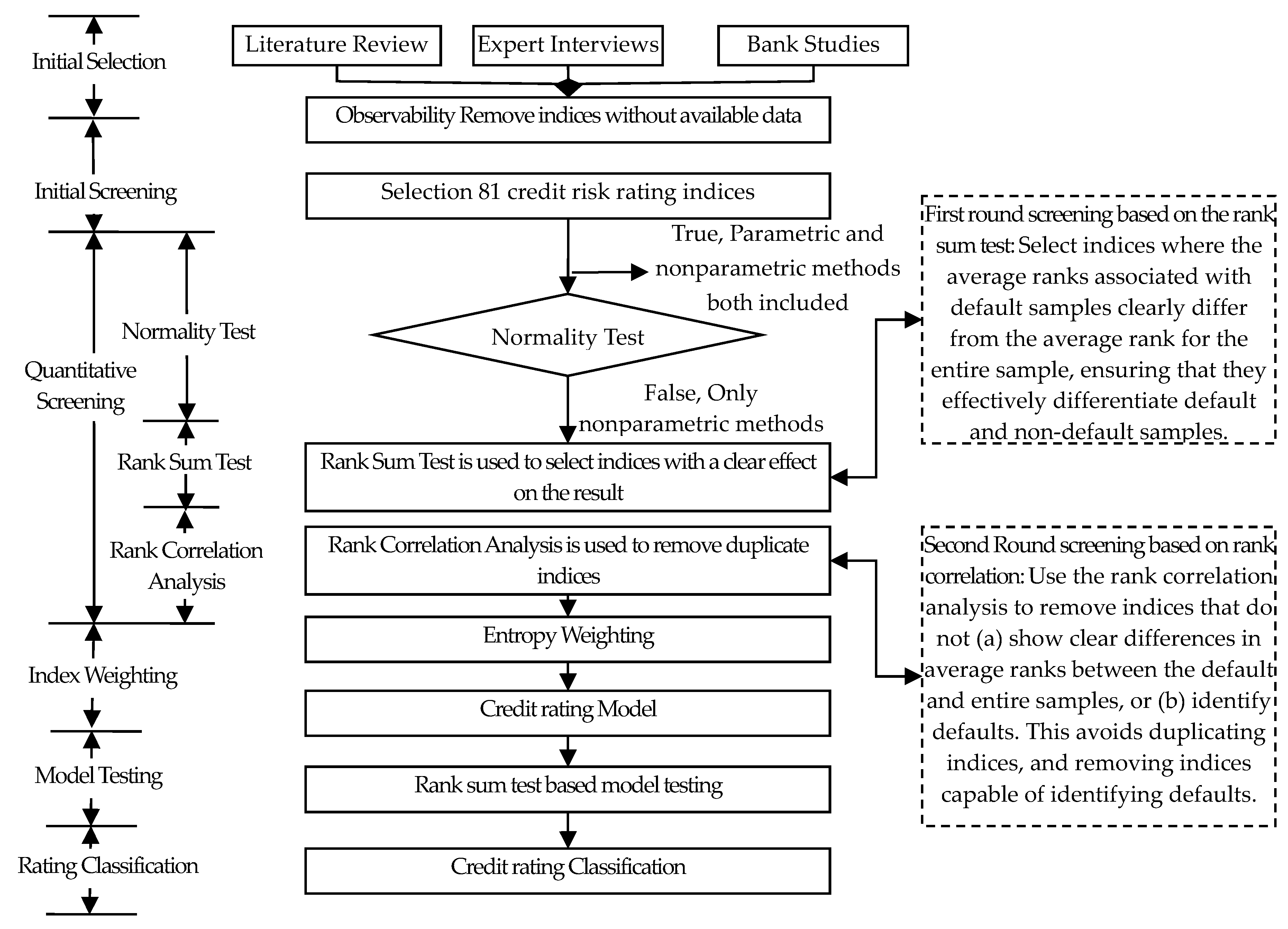
In this section, we introduce the process of creating a credit rating model based on a nonparametric method, including the rank sum test and rank correlation. A step-by-step instruction is provided, with the conceptual model for constructing the small enterprise credit rating model summarized in Figure 1.

To identify default enterprises, we construct the credit rating model in three aspects.

First, we use the Mann–Whitney rank sum test to screen indices. Using the rank sum test to select indices where the average ranks are associated with default samples with the entire sample showing a clear difference between them, ensuring that the chosen indices are able to clearly differentiate between the default and non-default samples. If the rank averages for default samples are significantly different from that of the entire sample, it means that the index is capable of clearly differentiating between the default and non-default samples, implying it can differentiate between defaults and non-defaults.

Second, we use the Spearman rank correlation coefficient method to remove duplicate indices. Using the rank correlation analysis, we remove the indices without showing a clear difference in average ranks between the default and entire samples, failing to clearly differentiate defaults. This avoids the problem of duplicate indices, and also avoids the removal of those differentiating defaults.

Third, we use the entropy value to give weight to each index; the more information an index has, the larger the weight should be given. Then, we define the critical point of credit score S_c, enterprises whose credit scores are lower than S_c to be classified as “default”, and those whose credit scores are higher than S_c to be classified as “non-default”. Thus, we classify the enterprises and identify the default.

2.1. Small Enterprise Credit Rating Index System

The construction of credit rating index system contains four steps. First we standardize the indices to eliminate the effects of different indicator dimensions. Next, we use the normal distribution test to check the distribution of the indices across the entire dataset. Then, in the first round screening, we select indices that have a clear effect on small enterprise defaults. Finally, we remove duplicate indices at the same criterion level, thereby ensuring a parsimonious index system through the second round screening.

2.1.1. Standardization of Index Data

Standardizing quantitative indices involves translating the indices to the [0,1] region and eliminating the effect of data dimensions on the rating result. There are three types of quantitative indices: positive indices, negative indices, and interval indices. A positive index is an index that is positively correlated with the credit rating of a small enterprise, such as the super quick ratio. A negative index is an index that is inversely correlated with the credit rating of a small enterprise, such as the asset/liability ratio. An interval index is an index for which a certain region of values [q₁, q₂] is optimal. As such, the closer an enterprise’s value to that index is to that region, the higher that enterprise’s credit rating will be.

Index data standardization process for the four types of indices is as follows. Let x_ij be the standardized value of the j-th sample in the i-th index, v_ij be the real value of the j-th sample in the i-th index, and N be the number of small enterprises. Given these definitions, the standardization equations of positive indices and negative indices are represented by Equations (1) and (2), respectively [33,34].

$$x_{ij}=\frac{v_{ij}-\underset{1\le i\le N}{\min }(v_{ij})}{\underset{1\le i\le N}{\max }(v_{ij})-\underset{1\le i\le N}{\min }(v_{ij})}$$

(1)

$$x_{ij}=\frac{\underset{1\le i\le N}{\max }(v_{ij})-v_{ij}}{\underset{1\le i\le N}{\max }(v_{ij})-\underset{1\le i\le N}{\min }(v_{ij})}$$

(2)

Let q₁ and q₂, respectively, represent the lower and the upper boundaries of the optimal region. Given this, the standardized score equation of the interval indices is expressed in Equation (3).

$$x_{ij}=\{\begin{array}{ccc}1-\frac{q_1-v_{ij}}{\max (q_1-\underset{1\le i\le N}{\min }(v_{ij}),\underset{1\le i\le N}{\max }(v_{ij})-q_2)},& v_{ij}<q_1\hfill & (3\mathrm{a})\\ 1-\frac{v_{ij}-q_2}{\max (q_1-\underset{1\le i\le N}{\min }(v_{ij}),\underset{1\le i\le N}{\max }(v_{ij})-q_2)},& v_{ij}>q_2\hfill & (3\mathrm{b})\\ 1,& q_1\le v_{ij}\le q_2\hfill & (3\mathrm{c})\end{array}$$

Because it is not easy to quantify qualitative indices, standardization uses subjective descriptions of the indices to obtain a rating. More specifically, standardization requires establishing a rating standard that can be manipulated while mitigating subjective factors.

Table 1. Standardized qualitative indices.

(1) No.	(2) Criterion Layer	(3) Index	(4) Description	(5) Standardized Value
1	X1 Internal non-financial factors	X1,1 Years in related industry	greater than 8 years (inclusive) 5 years (inclusive) to 8 years 2 years (inclusive) to 5 years less than 2 years, or lack of data	1.00
				0.70
				0.40
				0.00
…		…	…	…
8		X1,8 Famous brand level	main product is national famous brand main product is provincial famous brand main product is municipal famous brand main product is county famous brand other, or lack of data	1.00
				0.75
				0.50
				0.25
				0.00
…	…	…	…	…
20	X4 Commercial Reputation	X4,1 Enterprise tax records	at least 3 years of tax records with no tax delinquency records less than 3 years of tax records with no tax delinquency records individual tax delinquency record later paid in full no tax records two or more tax delinquency records, or lack of data	1.00
				0.75
				0.50
				0.25
				0.00
…		…	…	…
23		X4,4 Breach of contract	0 breaches of contract 1 breach of contract 2 breaches of contract 3 or more breaches of contract, or lack of data	1.00
				0.60
				0.30
				0.00

provides the rating systems for all 23 qualitative indices.

2.1.2. Normal Distribution Test for Rating Indices

Most determinations of normality rely on either the Shapiro–Wilk test or the K-S test. For a sample size between 3 and 2000, it is possible to test a distribution for normality using the Shapiro–Wilk method [35]. Our sample falls within this range, so we use the Shapiro–Wilk test to determine the distribution of the indices across the entire dataset. The value W is given by [36]:

$$W=\frac{{\left({\displaystyle \sum _{j=1}^N{a}_j}{x}_{i(j)}\right)}^2}{{\displaystyle \sum _{j=1}^N(}{x}_{i(j)}-{\overline{x}}_i{)}^2}$$

(4)

where a_j is a constant, and can be found in the Shapiro–Wilk weight table. x_i(j) is the j-th sample ranked in ascending order according to index i, and ${\overline{x}}_i$ is the average sample value for index i. Values for W range from 0 to 1, with higher values indicating a closer fit to a normal distribution.

Given confidence level α, if the two tails for W show a significance probability P(|W| > W_α/2) < α, then the sample does not possess a normal distribution. However, the empirical results below show that no index satisfies the conditions for a normal distribution, so traditional statistical methods are not suited for this sample set.

2.1.3. First Round Screening Based on the Rank Sum Test

In the first round, we select indices that have a clear effect on small enterprise defaults and that demonstrate clear differences between the average ranks associated with the default and entire samples to ensure that those indices can effectively differentiate default and non-default samples. We begin by ranking without identical ratings. Given index i, take m default samples and n non-default samples, and rank the m + n data samples from smallest to largest. Then, each sample x_ij (1 ≤ j ≤ m + n) has an associated rank R_ij in the combined dataset. If there are identical values after ordering the combined samples (which imply identical ranks), then we take the average rank from the associated ranks, and obtain the corrected rank $\overline{R_{ij}}$.

$$\overline{R_{ij}}={\displaystyle \sum _{}^h{R}_{ij}}/{\tau }_{ih},h=1,2,\dots ,g$$

(5)

where $\overline{R_{ij}}$ is corrected rank for the j-th sample in the i-th index, R_ij is the original rank for the j-th sample in the i-th index, and ${\tau }_{ih}$ is the length of the h-th identical rating rank column for the i-th index.

We next calculate the rank sum. Let W_iX be the rank sum of all default samples in the i-th index, $R^{\left(v\right)}{}_{iX}$ be the rank of the v-th default sample in index I, ${\sigma }_{iX}$ be the standard deviation for the rank of sum the default samples in index i, m be the number of default samples, n be the number of non-default samples, R_iE be the average rank for all samples in the index, and W_i be the rank sum for all samples in index i. Given these definitions, we obtain [2]:

$$W_{iX}={\displaystyle \sum _{v=1}^m{R}^{\left(v\right)}{}_{iX}}$$

(6)

$${\sigma }_{iX}=\sqrt{\frac{mn(m+n+1)}{12}}$$

(7)

$$R_{iE}=\frac{W_i}{m+n}=\frac{(m+n+1)}{2}$$

(8)

For a rank sum with identical ratings, let $\overline{R^{\left(v\right)}{}_{iX}}$ be the corrected rank for the v-th default sample in index i, ${\tau }_{ih}$ be the length of the h-th identical rating rank in index i, g be the total number of identical rating ranks, and the remaining variables defined as they are for Equations (6)–(8). Provided these definitions, we arrive at [2]:

$$W_{iX}={\displaystyle \sum _{k=1}^m\overline{R^{\left(v\right)}{}_{iX}}}$$

(9)

$${\sigma }_{iX}=\sqrt{\frac{1}{12}mn(m+n+1)-\frac{mn\left({\displaystyle \sum _g}({({\tau }_{ih})}^3-{\tau }_{ih})\right)}{12(m+n)(m+n-1)}}$$

(10)

For statistical inferences, we first establish the null and alternative hypotheses:

H₀: $W_{iX}=m{R}_{iE}$, in which both sample groups come from the same set, and the default and entire sample do not differ, indicating that the index does not effectively identify defaults.

H₁: $W_{iX}\ne m{R}_{iE}$, in which the two sample groups come from different sets, and the default and entire sample differ, indicating that the index effectively identifies defaults.

We next calculate and define the Z-statistic, such that [2]:

$$Z_i=\frac{W_{iX}-m{R}_{iE}}{{\sigma }_{iX}}$$

(11)

By dividing both the numerator and denominator in Equation (11) by the number of defaults m, we obtain Equation (12):

$$Z_i=\frac{W_{iX}/m-R_{iE}}{{\sigma }_{iX}/m}$$

(12)

The first variable in the numerator in Equation (12) is the average rank of all default samples. The second variable is the average rank of the entire sample R_iE. A large difference between these two variables indicates a large difference in the correlated values for the default and entire samples, and by extension, a greater value for Z. A high value for Z indicates that an index effectively distinguishes raw data into default and non-default samples, and can more easily identify defaults.

Because the distribution for Z is close to normal (i.e., N[0,1]; Wang, 2005), a high value for Z suggests that H₀ is likely to be rejected in favor of H₁. Given a significance level α, if the probability of the two tails of the Z distribution being significant is P(|Z| > Z_α/2) > α, the null hypothesis is rejected. To illustrate, if the significance level α = 0.01 [37], and the probability of significance is p > 0.01, then the index should be removed. If p > 0.01, then the index should be retained.

Thus, the value of Z reflects the level of difference between the average ranks of the default and entire sample such that greater Z values reflect larger differences between the samples (and by extension, larger differences between values for default and non-default samples). We chose indices that pass the Z value significance test to establish a credit rating index system capable of differentiating default and non-default samples.

2.1.4. Second-Round Screening Based on Rank Correlation Analysis

This round of screening removes duplicate indices at the same criterion level, thereby ensuring a parsimonious index system. If the sample values show identical increase and decrease trends under index k (i.e., return on equity) and index l (i.e., return on total assets), then indices k and l are fully correlated, and they provide redundant information; otherwise, indices k and l are weakly correlated, and thus provide information that is not redundant. By removing indices that provide duplicate information, we remove indices with a small absolute value for Z that does not effectively identify defaults.

To calculate the rank correlation coefficient, we rank the observed values for the entire sample under index k in ascending order, $R_1^k,R_2^k,\dots ,R_N^k$. We similarly rank the observed values for the entire sample for index l, $R_1^l,R_2^l,\dots ,R_N^l$. We then use these two series of rank orders to evaluate the differences in rank for observed values in indices k and l, and calculate d_u, to measure the correlation between the indices. The method for calculating d_u is as follows:

$$d_u=R_u^k-R_u^l,u=1,2,\dots ,N$$

(13)

where $R_u^k$ is the rank of the u-th sample in index k and $R_u^l$ is the rank of the u-th sample in index l. Given this, the rank correlation coefficient ${\gamma }^s$ is [2]:

$${\gamma }^s=\frac{\frac{N^3-N}{6}-\frac{1}{12}\left[{\displaystyle \sum _{G^k}^{}\left({({\tau }_g^k)}^3-{\tau }_g^k\right)}+{\displaystyle \sum _{G^l}^{}\left({({\tau }_g^l)}^3-{\tau }_g^l\right)}\right]-{\displaystyle \sum _{u=1}^n{d}_u^2}}{2\sqrt{\left[\frac{N^3-N}{12}-\frac{1}{12}{\displaystyle \sum _{G^k}^{}\left({({\tau }_g^k)}^3-{\tau }_g^k\right)}\right]\left[\frac{N^3-N}{12}-\frac{1}{12}{\displaystyle \sum _{G^l}^{}\left({({\tau }_g^l)}^3-{\tau }_g^l\right)}\right]}}$$

(14)

where, ${\tau }_g^k$ and ${\tau }_g^l$ are the respective lengths of the g-th section in indices k and l, and G^k and G^l are the number of ranks with identical ratings. From here, we can determine t using Equation (15):

$$t={\gamma }^s\sqrt{\frac{N-2}{1-{\gamma }^{s2}}}$$

(15)

Provided a given significance level α, if t is greater than t_α, then the two samples are correlated in terms of the two indices, indicating that they provide duplicate information. Because indices can easily pass the rank correlation significance test when sample size is large, we set a rank correlation coefficient condition to ensure the indices provide duplicate information. Generally, two conditions must be satisfied to infer that indices produce similar information. First, p must be greater than the established significance level (typically, α = 0.01). Second, the rank correlation coefficient ${\gamma }^s$ must be greater than 0.6 [38]. To remove indices that produce redundant information, we select the indices in the same criterion level that satisfy the above conditions, and remove those indices that have relatively small absolute values for Z that do not clearly identify defaults.

2.2. Establishing the Small Enterprise Credit Rating Model

This part contains a series of steps, including entropy weighting, credit rating equation construction, the test of the model’s effectiveness and the division of small enterprise credit ratings.

Entropy weighting is an objective weighting method that uses the entropy value for an index to represent the amount of information it provides. To calculate entropy values, let e_i represent the entropy value for the i-th rating index; Equations (16) and (17) provide the formulae for calculating e_i [39]:

$$f_{ij}=\raisebox{1ex}{$x_{ij}$}\!\left/ \!\raisebox{-1ex}{${\displaystyle \sum _{i=1}^n{x}_{ij}}$}\right.$$

(16)

$$e_i=\frac{1}{\ln n}{\displaystyle \sum _{i=1}^N{f}_{ij}}\ln f_{ij}$$

(17)

where f_ij is the eigenweight for the j-th sample in index i, x_ij is the observed value for the j-th sample in index i (i = 1, 2, …, n; j = 1, 2, …, m), and ${\displaystyle \sum _{i=1}^N{x}_{ij}}$ is the sum of the observed values for all samples in index i. We next calculate the entropy weights for each index. Let w_i be the entropy value for the i-th rating index; the entropy rating is then given by:

$$w_i=\frac{1-e_i}{n-{\displaystyle \sum _{i=1}^N{e}_i}}$$

(18)

Given index i, larger values for x_ij indicate that an index effectively compares to sample j. Moreover, larger values for x_ij indicate that more index i includes more information, thereby validating the greater weight assigned to x_ij.

In the credit rating equation for small enterprises, let p_j be the credit rating for the j-th small enterprise. According to the linear weighting comprehensive rating equation, the credit rating model for small enterprises is:

$$p_j={\displaystyle \sum _{i=1}^m{w}_i{x}_{ij}}$$

(19)

The value of the credit rating for small enterprises p_j as solved for in Equation (19) is in the region [0,1], which is too small to clearly reflect differences in credit ratings for small enterprises. Thus, p_j must be standardized to the region [0,100]. Let S_j be the standardized credit rating for the j-th small enterprise. Because higher small enterprise credit ratings imply higher standardized credit ratings, let the standardized credit rating for small enterprises be given by:

$$S_j=\frac{p_j-\underset{1\le j\le n}{\min }(p_j)}{\underset{1\le j\le n}{\max }(p_j)-\underset{1\le j\le n}{\min }(p_j)}\times 100$$

(20)

To determine the effectiveness of the small enterprise credit rating model in differentiating between default and non-default samples, we test whether there is a clear difference between average ranks associated with the default and entire samples. If the average rank of the credit rating for default samples is clearly different from the average rank of the entire sample, then the model clearly differentiates between default and non-default samples in terms of credit rating.

To perform the rank sum test, we must rank the credit ratings for all samples, calculate the rank sum, and test the average ranks associated with the ratings as described in Section 2.1.3. Given a significance level α of 0.01 [37], if p < 0.01, then default and non-default samples clearly differ in terms of credit rating, and the model is capable of differentiating between these two types of samples. This not only ensures that individual indices can effectively predict defaults, but also that the entire small enterprise credit rating model can effectively identify defaults by small enterprises.

After the test of the model’s effectiveness, we rank the standardized credit ratings for every small enterprise in descending order. Using data on the principal and interest on accounts outstanding and receivable for each small enterprise, we divide credit rating into nine levels [40], and calculate the Loss Given Default (LGD) for each level.

According to results produced by our research group [41], by adjusting the upper and lower bounds of the nine credit rating levels to ensure a strong inverse relationship between credit rating and LGD, we determine that the optimal result is the one for which there is the smallest difference between adjacent credit rating levels.

3. Empirical Study: Data from a Chinese Bank

3.1. Sample and Data Source

According to the Standards for Classification of Small and Medium-sized Enterprises [42], we collected small enterprise sample data across 11 industries, which can be seen in

Table 2. Chinese small enterprise standards.

(1) No.	(2) Industry	(3) Small Enterprise Classification
1	Retail	10–50 employees, 1–5 million RMB operating income
2	Wholesale	5–20 employees, 10–50 million RMB operating income
3	Construction	3–60 million RMB operating income, 3–50 million RMB total assets
4	Warehousing	20–200 employees, 1–10 million RMB operating income
5	Information Services	10–100 employees, 1–10 million RMB operating income
6	Transportation	20–300 employees, 2–30 million RMB operating income
7	Accommodation and catering	10–100 employees, 1–20 million RMB operating income
8	Leasing and business services	10–100 employees, 1–80 million RMB total assets
9	Real estate development and management	1–10 million RMB operating income, 20–50 million RMB total assets
10	Software and information technology	10–300 employees, 0.5–100 million RMB operating income
11	Other	10–100 employees

. These industries included, but were not limited to, real estate development and management, retail, leasing and business services, wholesale, accommodation and catering, transportation, software and information technology.

Our data provided information related to 1231 loans to small enterprises from a Chinese bank between 1994 and 2012. Of the 1231 loans in the dataset, 35 were defaults and 1196 were non-defaults. All data associated with the 1231 loans are summarized in Columns 1 to 1231 in

Table 3. Original and standardized data for the 81 small enterprises indices.

(a) No.	(b) Criterion Level	(c) Index	(d) Index Type	Original Data for the 1231 Loans vij			Standardized Data for the 1231 Loans xij			(e) Normality Test Value p	(f) Z
				(1) 2004100 90044	…	(1231) X201 2060800099	(1232) 200 410090044	…	(2462) X201 2060800099
1	C1 Solvency	X1 Debt ratio	Negative	0.640	…	0.603	0.454	…	0.369	0.00	−1.526
2		X2 Current liabilities, operating activities and net cash flow ratio	Positive	1.125	…	0.136	0.472	…	0.496	0.00	−1.269
…		…	…	…	…	…	…	…	…	…	…
20		X20 EBITDA/current liabilities ratio	Positive	0.031	…	0.059	0.052	…	0.010	0.00	−3.361
21	C2 Profitability	X21 Return on equity	Positive	0.055	…	0.067	0.232	…	0.065	0.00	−2.885
…		…	…	…	…	…	…	…	…	…	…
24		X24 return on total assets	Positive				0.026		0.003	0.00	−3.756
…	C2 Profitability	…	…	…	…	…	…	…	…	…	…
33		X33 Cash inflows from operating activities	Positive	62 816 920	…	592 213 568	0.005	…	0.026	0.00	−2.349
34	C3 Operating Capacity	X34 Accounts receivable turnover	Positive	1.937	…	18.000	0.015	…	0.054	0.00	−3.670
…		…	…	…	…	…	…	…	…	…	…
43		X43 Cash conversion cycle	Negative	-2.546	…	17.230	0.502	…	0.509	0.00	−1.999
44	C4 Growth Capacity	X44 Revenue growth	Positive	0.000	…	0.130	0.197	…	0.222	0.00	−0.417
…		…	…	…	…	…	…	…	…	…	…
48		X48 Retained earnings growth	Positive	1.809	…	0.888	0.519	…	0.513	0.00	−1.001
49	C5 External Macroeconomic Conditions	X49 Industry sentiment index	Positive	127.960	…	123.300	0.695	…	0.579	0.00	−4.969
…		…	…	…	…	…	…	…	…	…	…
54		X54 Engel coefficient	Negative	39.400	…	36.200	0.651	…	0.790	0.00	−7.187
55	C6 Internal Non-financial factors	X55 Years in industry	Qualitative	9 years	…	10 years	0.000	…	1.000	0.00	−2.528
…		…	…	…	…	…	…	…	…	…	…
63		X63 Ratio of loans repaid	Positive	0.000	…	1.000	0.000	…	1.000	0.00	−2.769
64	C7 Legal Person Situation	X64 Education background	Qualitative	N/A	…	Bachelors	0.700	…	1.000	0.00	−0.462
…		…	…	…	…	…	…	…	…	…	…
71		X71 Age	Interval	N/A		38	0.000		1.000	0.00	−1.246
…		…	…	…	…	…	…	…	…	…	…
74		X74 Time in current position	Qualitative	10	…	4	0.000	…	0.400	0.00	−4.923
75	C8 Enterprise Credit Situation	X75 Registered capital classification	Qualitative	N/A	…	Fund	0.800	…	1.000	0.00	−2.315
76		X76 Credit received in past 3 years	Qualitative	Records of default, outstanding loans	…	Credit records, non-default	0.000	…	1.000	0.00	−5.699
77	C9 Commercial Reputation	X77 Tax Records	Qualitative	No tax records	…	3 or more years of tax records, no tax delinquency records	0.250	…	1.000	0.00	−2.231
…		…	…	…	…	…	…	…	…	0.00	…
80		X80 No. of breaches of contract	Qualitative	0 breaches of contract	…	0 breaches of contract	1.000	…	1.000	0.00	−4.239
81	C10 Collateral Guarantee Factor	X81 Collateral Guarantee Rating	Qualitative	Industrial land use rights	…	Other enterprise guarantee	0.669	…	0.570	0.00	−4.540
82	——	Default	——	1.000	…	0.000	1.000	…	0.000	0.00	-

. For simplicity, we divide the data such that Columns 1232 to 1266 contain data for the 35 defaults, and Columns 1267 to 2462 contain data associated with the 1196 non-defaults. To simplify the data even further, Row 82 in Table 3 serves as a default indicator where a value of 1 represents a default, and a value of 0 represents a non-default.

3.2. Establishing the Credit Rating Index System

Using index data from the main office of a Chinese national bank, small enterprise index systems from domestic and international financial agencies (i.e., Moody, Standard and Poor’s, and the China Construction Bank), classic ratings indices from domestic and international academic resources, and survey data collected from real-world banks, we collected a sample of 107 small enterprise credit rating indices for screening. The index names, types, and references are listed in Columns 5, 6, and 7 of

Table 4. Index system selection for small enterprise credit rating.

(1) No.	(2) 1st Level Criteria	(3) 2nd Level Criteria	(4) 3rd Level Criteria	(5) Index Name	(6) Type	(7) References	(8) Screening Result
1	Repayment Ability	Internal Financial Factors	Solvency	Debt ratio	Negative	[3,5,6,8,14]	Failed rank sum test
2				Current liabilities, operating activities and net cash flow ratio	Positive	[4,5,6,10,14]	Failed rank sum test
…				…	…	…	…
28				Source of repayment	Qualitative	[7,11,12,13]	Unobservable
29			Profitability	Return on equity	Positive	[3,4,5,6,8,10,11,12,13,14,15]	Failed rank correlation analysis test
30				Sales, net present value rate	Positive	[5,6,7,8,10,13]	Failed rank sum test
…				…	…	…	…
44				Earnings per share	Positive	[3,8,11]	Unobservable
45			Operating Capacity	Accounts receivable turnover	Positive	[4,5,6,7,8,12,14]	Failed rank correlation analysis test
…				…	…	…	…
54				Cash conversion cycle	Positive	[4,5,6,10,12,13]	Failed rank sum test
55			Growth Capacity	Revenue growth	Positive	[4,7,8,9,11,15]	Failed rank sum test
…				…	…	…	…
63				Salary and benefits growth	Positive	[13]	Unobservable
64		External Macroeconomic Conditions		Industry sentiment index	Positive	[3,4,5,6,10,11,12,13]	Pass
…				…	…	…	…
72				Economic environment	Qualitative	[9,13]	Unobservable
73		Internal Non-financial factors		Years in industry	Qualitative	[6,8,9,10,12,13,14]	Failed rank sum test
…				…	…	…	…
85				Management level	Qualitative	[8,9,15]	Unobservable
86	Willingness to repay	Legal Person Situation		Legal person education background	Qualitative	[8,10,11,12]	Failed rank sum test
…				…	…	…	…
98				Owner qualities	Qualitative	[4,9,12,15]	Unobservable
99		Enterprise Situation		Registered capital classification	Qualitative	[3,4,5,6,10,12]	Failed rank sum test
…				…	…	…	…
102				Customer complaint rate	Qualitative	[12]	Unobservable
103		Commercial Reputation		Tax records	Qualitative	[3,8,9,10,15]	Failed rank sum test
104				Legal disputes	Qualitative	[5,6,7,8,10,13]	Failed rank correlation analysis test
…				…	…	…	…
106				No. of breaches of contract	Qualitative	[3,4,5,9,10,11,12]	Pass

.

The selection set encompasses three first-level criteria (i.e., repayment ability, willingness to repay, and collateral guarantee factors), seven second-level criteria: external macroeconomic conditions, internal non-financial factors, legal person situation, and internal financial factors, which is further divided into four third-level criteria including solvency, profitability, operating capacity, and growth capacity. Columns 2–4 of Table 4 outline these criteria.

Based on the observability principle, we performed a preliminary screening of the 107 indices, during which we removed 26 indices, including “source of repayment” and “earnings per share”. These indices are labeled “Unobservable” in Column 8 of Table 4. These removals yielded a final set of 81 indices, displayed in Column c of Table 3, ensuring our rating system is practicable. In addition, the first 81 rows and Columns 1–1231 of Table 3 illustrate the raw data associated with v_ij for the j-th sample in index i. From these data, we can calculate the maximum value $\max (v_{ij})$ and minimum value $\min (v_{ij})$ for each row.

For positive indices (“positive” in Column d in Table 3), we substituted their v_ij, $\max (v_{ij})$, and $\min (v_{ij})$ into Equation (1) and entered the standardized values x_ij into their respective columns (1232–2462). For negative indices (negative in Column d, Table 3), we substituted their v_ij, $\max (v_{ij})$, and $\min (v_{ij})$ into Equation (2) and entered the standardized values x_ij into Columns 1232–2462.

Interval indices are indicated in Column d of Table 3 with the term “interval”. To illustrate the standardization process, consider “Age” in Row 71 of Table 3. The age of the legal person associated with loan X2012060800099 in Column 1231 is 38, which is within the optimum interval [31]. According to Equation (3c), this makes the standardized value x_ij of “Age” in this case equal to 1. Thus, we entered this value into the cell located at Row 71, Column 2462 of Table 3. We standardized the Consumer Price Index using the same process.

For qualitative indices (“qualitative” in Column d of Table 3), we used the qualitative index rating classification provided in Table 1 to obtain the standardized result x_ij, which we then entered into Columns 1232–2462 of Table 3. Consider, for example, the “Years in industry” variable from Row 55 in Table 3. The years in industry associated with loan X2012060800099 from Column 1231 is 10 years. According to Table 1, this value is standardized such that it is equal to 1, which we then entered into Row 55, Column 2462 of Table 3. We standardized all other qualitative indices in a similar fashion.

We performed a normal distribution test for indices 1–81 in Table 3 and illustrate the results using “X₁ Debt ratio”. First, we ranked the 1231 sample values from Row 1, Columns 1–1231 of Table 3 in ascending order to obtain x_1(j), from which we determined the average sample rank ${\overline{x}}_1$ to be 1.106. Using a_j for each sample (n = 1231), we substituted x_1(j), ${\overline{x}}_1$, and a_j into Equation (4), obtaining W₁. Given a confidence level α of 0.01, we obtained a significance probability of 0.000 for both tails for W₁, which we then entered into Row 1, Column e of Table 3. Column e of Table 3 shows that the tests of normality for all indices produced p-values of less than 0.01, thereby allowing us to reject the null hypothesis that all indices possess a normal distribution and accept that all 81 rating indices for these small enterprises are non-normally distributed.

3.2.1. First Round Screening Based on the Rank Sum Test

We performed the rank sum test on all 81 indices listed in Column c of Table 3 using the “X₁ Debt ratio” as above to illustrate how we calculated Z. First, we combined the respective data from Row 1 of Table 3 for the 35 default loans in Columns 1232–1266 and the non-default loans from Columns 1267–2462. We then ranked loans in ascending order and entered them into Column 3 of

Table 5. Ranking of small enterprise loans.

(1) No.	(2) Loan No.	(3) Debt Ratio	(4) Default?	(5) Order No.	(6) Length	(7) Rank
1	200412150123	0	1	1	76	38.5
2	200512220004	0	1	2		38.5
…	…	…	…	…		…
76	X2011122100005	0	0	76		38.5
77	200909230014	0.0004	0	77	3	78
…	…	…	…	…	…	…
1228	200902180021	1	0	1228	4	1229.5
1229	E2010033100036	1	0	1229		1229.5
1230	E2011070600042	1	0	1230		1229.5
1231	E2011080500001	1	0	1231		1229.5

.

We then substituted the data from Rows 1–76, Columns 5–6, in Table 5 into Equation (5), and corrected the ranks for samples with a debt ratio of 0 to:

$${\overline{R}}_{1-76}={\displaystyle \sum _{j=1}^{76}(1+2+}\cdots +76)/76=38.5$$

We then entered the results into Column 7, Row 1–76 of Table 5 and substituted the rank associated with a default indicator value of 1 (see Column 4 of Table 5) into Equation (9). This produced the rank sum W_1X for sample X₁:

$$W_{1X}={\displaystyle \sum _{j=1}^{35}(38.5+38.5+}\cdots +1203)=18,396.5$$

We then substitute m = 35, n = 1196, and W_1X = 18,396.5 into Equation (8) to obtain the average rank R_1E for the entire sample:

$$R_{1E}=\frac{(35+1196+1)}{2}=616$$

Because identical ranks emerged, we substituted the above m, n, and length τ_g into Equation (10) to obtain the rank sum variance σ_1X for the default samples.

$$\begin{array}{ll}{\sigma }_{1X}& =\sqrt{\frac{1}{12}\times 35\times 1196\times 1232-\frac{35\times 1196\left(\left({76}^3-76\right)+\left(3^3-3\right)+\cdots +\left(4^3-4\right)\right)}{12\times 1231\times 1230}}\\ & =2072.79\end{array}$$

We then substituted the rank sum W_1X, average rank R_1E and rank sum variance σ_1X for sample X₁ into Equation (11). Given this, we calculated Z₁:

$$Z_1=\frac{18,396.5-35\times 616}{2072.29}=-1.526$$

We entered Z₁ into Row 1, Column f of Table 3. Given a confidence level α of 0.01, and a p-value (with 1231 degrees of freedom) of 0.127 in the standard normal distribution table, we rejected the null hypothesis. This indicated that there was no significant difference between the ranks associated with the default and entire sample in terms of the debt ratio index. Because the debt ratio index could not clearly identify defaults (i.e., distinguish defaults from the overall sample), we removed it from the model. We performed similar rank sum tests on the other 81 indices and removed 48. The indices removed from the model are labeled “Failed rank sum test” in Column 8 of Table 4.

3.2.2. Second Round Screening Based on Rank Correlation Analysis

For each of the 33 indices that passed the rank sum test, we performed rank correlation analyses on the entire sample set with the indices at the same criterion level. To illustrate this process, we offered the rank correlation analysis process for the “return on equity” and “return on total assets” indices. We ranked the values for the “return on equity” index in ascending order to obtain the index rank R_i^k. We then did the same for the “return on total assets” index to reveal rank R_i^l. Columns 3–4 in

Table 6. Rank differences for loans to small enterprises.

(1) No.	(2) Loan No.	(3) Rik	(4) Ril	(5) di	(6) di2
1	200410090044	529	467	62	3844
2	200410270004	609	539	70	4900
…	…	…	…	…	…
1230	X2012052200034	302.5	327.5	-25	625
1231	X2012060800099	302.5	327.5	-25	625

summarize these results.

We then substituted the data from Columns 3–4 in Table 6 into Equation (13), thereby obtaining an observed difference in rank using:

$$d_1=R_1^k-R_1^l=529-467=62$$

where d₁² = 62² = 3844. We then similarly solved for the rank differences d_i and squares d_i² for the other rows of Table 6, and entered the values into Columns 5 and 6.

We followed this by substituting d_i² from Column 6 of Table 6 and N = 1231 into Equation (14) to calculate the rank correction coefficient ${\gamma }^s$:

$$\begin{array}{l}{\gamma }^s=\frac{\frac{{1231}^3-1231}{6}-\frac{1}{12}({(277}^3-277)+\cdots {+(11}^3{-11)+(286}^3-286)+\cdots +{(3}^3-3))-(3844+\cdots +625)}{2\sqrt{\left[\frac{{1231}^3-1231}{12}-\frac{{(277}^3-277)+\cdots {+(11}^3-11)}{12}\right]\left[\frac{{1231}^3-1231}{12}-\frac{{(286}^3-286)+\cdots +{(3}^3-3)}{12}\right]}}\\ =0.834\end{array}$$

We then inserted ${\gamma }^s$ = 0.834 and N = 1231 into Equation (15) to obtain statistic t:

$$t=0.834\times \sqrt{\frac{1231-2}{1-{0.834}^2}}=52.99$$

Given a significance level α of 0.01, a t_α of 2.326, and the fact that t > t_α, the ranks for samples are correlated in terms of return on equity and return on total assets. Because the rank correlation coefficient γ^S = 0.834 > 0.6, we determined that the two indices provide duplicate information. According to Column f in Table 3, we removed the return on equity index because its absolute value of Z is less than that for the return on total assets index. We similarly calculated the rank correlation coefficient for the other criterion levels and removed indices with smaller absolute values for Z (see Column f of Table 3). In total, we removed 11 indices, which we labeled with “Failed rank correlation analysis test” in Column 8 of Table 4.

3.2.3. The Small Enterprise Index System and the Comparison with the Five Cs of Credit

The five Cs of credit is a system used by lenders to gauge the creditworthiness of potential borrowers, which has been widely used in the practice. The five Cs of credit are character, capacity, capital, collateral and conditions.

This study proposes a small enterprise credit rating index system that includes 22 indices covering all nine 3rd level criterion levels and satisfying the five Cs of credit. Columns e of

Table 7. The small enterprise index system and the comparison with the five Cs of credit.

(a) No.	(b) 1st Level Criteria	(c) 2nd Level Criteria	(d) 3rd Level Criteria	(e) Index	(f) Entropy Weighting	(1) Character	(2) Capacity	(3) Capital	(4) Collateral	(5) Condition
1	Repayment Ability	Internal Financial Factors	C1 Solvency	X5 Main business revenue/cash ratio	0.0418			√
2				X10 Super quick ratio	0.0394			√
3				X12 Net assets/year end loan balance ratio	0.0882		√
4				X13 Fixed capital ratio	0.0056		√
5				X15 Long term asset appropriation rate	0.1390		√
6				X20 EBITDA/current liabilities ratio	0.1284			√
7			C2 Profitability	X24 Return on total assets	0.0674		√
8				X27 Gross margins	0.0667		√
9			C3 Operating Capacity	X39 Shareholders’ equity turnover rate	0.0708			√
10			C4 Growth Capacity	X47 Capital accumulation rate	0.0006		√
11		C5 External Macroeconomic Conditions		X49 Industry sentiment index	0.0386					√
12				X52 Consumer Price Index	0.0697					√
13				X54 Engel coefficient	0.0437					√
14		C6 Internal Non-financial factors		X61 Sales reach	0.0467		√
15				X63 Ratio of loans repaid	0.0336		√
16	Repayment Ability	C7 Legal Person Situation		X66 Legal person credit card history	0.0499	√
17				X68 Residence status	0.0236		√
18				X69 Time spent in current residence	0.0261		√
19				X74 Time in current position	0.0016		√
20		C8 Enterprise Situation		X76 Credit received in past 3 years	0.0003	√
21		C9 Commercial Reputation		X80 No. of breaches of contract	0.0007	√
22	C10 Collateral Guarantee Factor			X81 Collateral Guarantee Rating	0.0174				√

is the indices we select. Columns 1–5 of Table 7 summarize the comparison between the five Cs of credit and the index system we build.

3.3. Solving for Small Enterprise Credit Rating

We inserted the data from Columns 1232–2462 in Table 3 into Equations (16)–(18) to obtain the entropy weighting for 22 post-screening indices. Upon obtaining them, we entered them into Column f in Table 7. We then substituted the data from Columns 1232–2462 in Table 3 and the weighting from Column f in Table 7 into Equation (19) to obtain the rating p₁ = 0.018 for loan 200410090044. Having obtained that rating value, we entered it into Row 1, Column 3 of

Table 8. Credit rating results for small enterprises.

(1) No.	(2) Loan No.	(3) Initial Credit Rating pj	(4) Standardized Credit Rating Sj	(5) Default	(6) Interest Receivable	(7) Outstanding Interest
1	200410090044	0.018	1.90	1	16964393	15100789
2	200410270004	0.253	46.36	0	13510055	0
…	…	…	…	…	…	…
1231	X2012060800099	0.360	66.49	0	2449108	0

. We calculated all other small enterprise credit ratings p_j, and entered them into Column 3 in Table 8. These steps provided us with the highest and lowest small enterprise credit ratings (p_max = 0.537 and p_min = 0.008, respectively).

We then entered the value 0.018 from Row 1, Column 3 into Table 8, and the highest (0.537) and lowest (0.008) ratings into Equation (20) to obtain the standardized credit rating for loan 200410090044,

S₁ = (0.018 − 0.008)/(0.537 − 0.008) × 100 = 1.90.

We entered this value into Row 1, Column 4 in Table 8, along with the standardized credit ratings S_i for all remaining small enterprises. Table 8, Column 5 shows whether a loan has defaulted, and Columns 6 and 7, respectively, illustrate the interest receivable and outstanding interest as provided by a commercial bank’s credit management database.

3.4. Model Validation

3.4.1. Testing the Small Enterprise Credit Rating Model with the Rank Sum Test

We ranked the credit ratings from Column 4 of Table 8 in ascending order and inserted them into Column 3 of

Table 9. Small enterprises credit ratings.

(1) No.	(2) Loan No.	(3)Score Sj	(4) Default	(5) Order No.	(6) Length	(7) Rank
1	199319010019001	0	1	1	3	2
2	199412010003501	0	1	2
3	199419010019101	0	1	3
…	…	…	…	…	…	…
1228	200710230043	98.781	0	1228	3	1229
1229	200711020006	98.781	0	1229		1229
1230	200711020007	98.781	0	1230		1229
1231	200904300004	100	0	1231	1	1231

. Columns 2 and 4 of Table 9 show the loan number and default indicator for each loan, respectively. In Column 5 of Table 9, and we determined the length of each identical rank and the final standardized rank, which we then inserted into Columns 6 and 7 of Table 9, respectively.

We then inserted the ranks of the defaults associated with a default indicator of 1 in Column 7 in Table 9 into Equation (9), thereby obtaining the default sample credit rating rank sum W_SX:

$$W_{SX}={\displaystyle \sum _{j=1}^{35}(2+2+}\cdots +561)=6367$$

Following this, we substituted m = 35, n = 1196 and W_SX = 6367 into Equation (8) to obtain the average rank of the credit ratings for the entire sample R_SX:

$$R_{SX}=\frac{(35+1196+1)}{2}=616$$

With identical ranks existing, we substituted m, n, and length τ_g into Equation (10) to obtain the default samples rank sum variance σ_SX:

$$\begin{array}{ll}{\sigma }_{SX}& =\sqrt{\frac{1}{12}\times 35\times 1196\times 1232-\frac{35\times 1196\left(\left(3^3-3\right)+\left(4^3-4\right)+\cdots +\left(3^3-3\right)\right)}{12\times 1231\times 1230}}\\ & =2071.41\end{array}$$

We next substituted the rank sum W_SX and average rank R_SX for default sample X_s, as well as the default sample rank sum variance σ_SX into Equation (11), thus obtaining Z_s:

$$Z_{\mathrm{s}}=\frac{6367-35\times 616}{2071.41}=-7.329$$

The p-value for the test of distribution normality (with 1231 degrees of freedom) was less than 0.01. Given an α value of 0.01, we rejected the null hypothesis. Therefore, our findings suggest that the ranks be associated with the default and that the entire sample demonstrate clear differences, therefore capable of differentiating defaults from non-defaults.

3.4.2. Comparison with Parametric Method

To validate the model we established, we compared the model we established with a parametric model. We followed the literature [43] and constructed a credit rating model based on t test and multiple discriminant analyses (MDA), with the t test model compared with the model we established.

Here we defined two models:

• Model 1: The model we constructed in this study.
• Model 2: Using t test for feature selection and the MDA for model construction.

For model 2, we used the t test for feature selection first. Given α = 0.05, we deleted the indicators whose p values of t test were greater than 0.05, and obtained 39 indicators reserved: X₂ Current liabilities, operating activities and net cash flow ratio, X₂₁ Return on equity, X₂₄ return on total assets and other 36 indicators.

Then we took the 39 indicators into the MDA method using the SPSS software, with the discriminant equation shown as follows.

$$D=2.23{\mathrm{X}}_2-1.021{\mathrm{X}}_3-0.098{\mathrm{X}}_4+\dots +1.049{\mathrm{X}}_{78}-0.271{\mathrm{X}}_{79}$$

(21)

We substituted the data from Table 3 into Equation (21), and achieved the default status prediction for each enterprise. By a comparison of the predicted default status and the true status, we can obtain the correct classification rate shown in Column 3 of

Table 10. Correct classification rates by Model 1 and Model 2.

	Model 1	Model 2
Correct default classification rate, 35 defaults	29/35 = 82.9%	22/35 = 62.9%
Correct non-default classification rate, 1196 non-defaults	946/1196 = 79.1%	1176/1196 = 98.3%
Correct overall classification rate	81.00% = (82.9% + 79.1%)/2	80.60% = (62.9% + 98.3%)/2

.

For Model 1, r to obtain the correct classification rate, we define the critical point of credit score S_c as [44]

$$S_c=\frac{\frac{1}{m}{\displaystyle \sum _{j=1}^m{S}_j^1}+\frac{1}{n}{\displaystyle \sum _{j=1}^n{S}_j^0}}{2}$$

(22)

where S_j¹ is the credit score of the i-th defaulted sample, m is the number of defaulted samples, S_j⁰ is the credit score of the j-th non-defaulted sample, and n is the number of non-defaulted samples.

Substitution of the data from Rows 1–1231, Columns 4, in Table 8 into Equation (22) yields the critical point S_c:

$$S_c=\frac{\frac{1}{35}{\displaystyle \sum _{j=1}^{35}{S}_j^1}+\frac{1}{1196}{\displaystyle \sum _{j=1}^{1196}{S}_j^0}}{2}=38.04$$

Enterprises with credit scores of less than 38.04 will be classified as “default”, and those with credit score of more than 38.04 will be classified as “non-default”.

Comparing the true status of default and the predicted status, we can obtain the correct classification rate either, as shown in Column 2 in Table 10.

From Row 1 of Table 10, it is clear that the Model 1 is more accurate in the default classification, with the correct default classification rate of Model 1 being 82.9%, which is higher than that of Model 2 (62.9%).

From Row 2 of Table 10, it can be seen that the Model 1 is less accurate in the non-default classification, with the correct non-default classification rate of Model 1 being 79.1%, which is lower than that of Model 2 (98.3%).

As is known, for each bank, the losses from a loan to unqualified enterprises are much greater than those from no loan to qualified enterprises. Although Model 1 and Model 2 have a similar overall classification rate (shown in Table 10), due to the more accurate prediction of the default, Model 1 outperformed Model 2.

Thus, Model 1 has a better performance than the t test-MDA model in dealing with the data of the small enterprises. As mentioned above, the parametric model relies on the normal distribution, but the small enterprises data used in this research are abnormal, so the result is biased when using the parametric method, especially in the default sample classification. That is also the reason for utilizing the nonparametric method in this study.

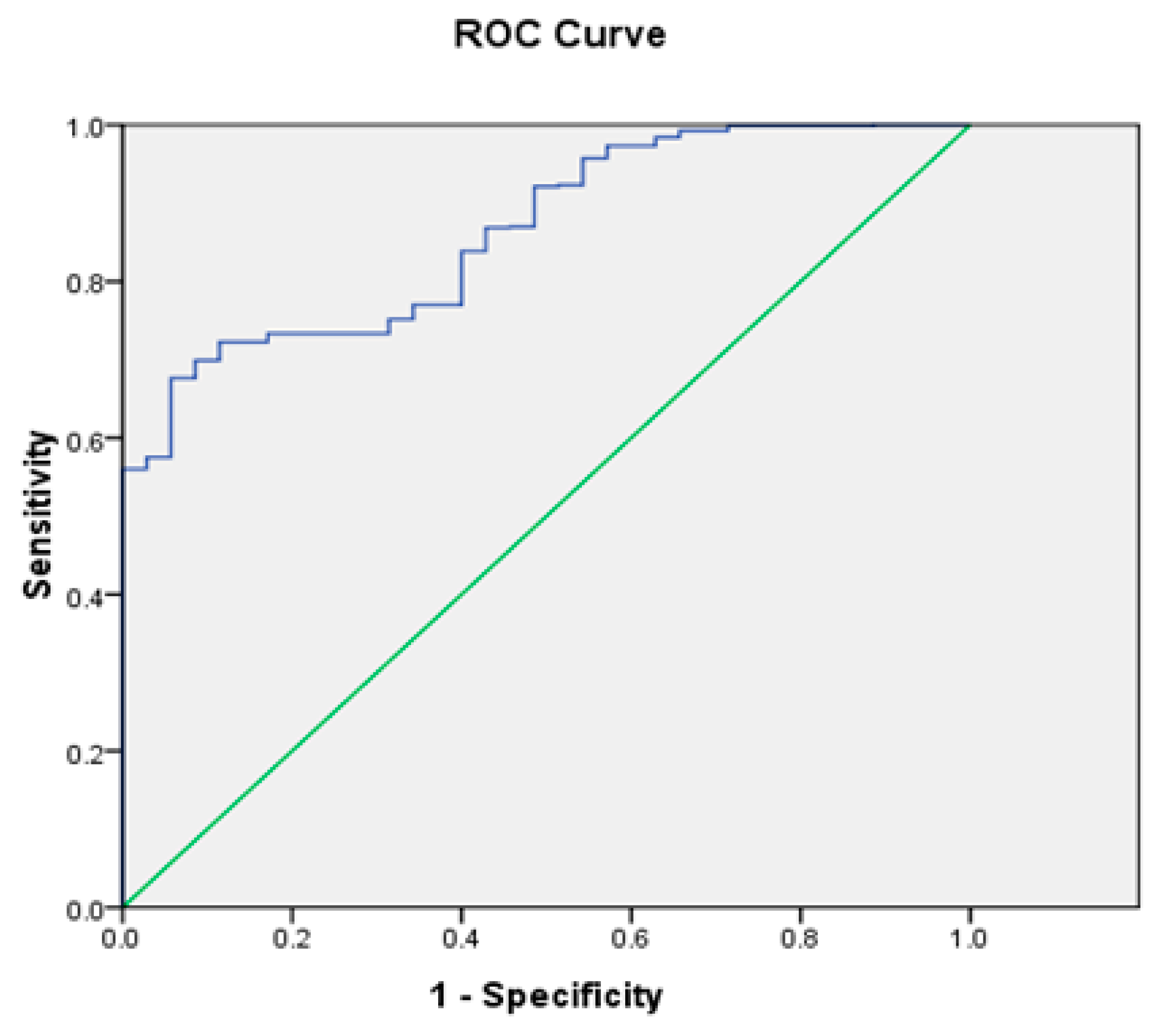
Furthermore, we inputted the rating score S_j and the default state to generate the Receiver Operating Characteristic curve (ROC curve) using SPSS software (see Figure 2). The Area Under Curve (AUC) value is 0.863, which is a acceptable level for credit rating model.

3.5. Classification of Small Enterprise Ratings

We ranked the credit ratings from Column 4 of Table 8 in descending order. According to the results of our research group [41], we introduced the interest receivable and interest outstanding from Columns 6 and 7 of Table 8 into the credit rating classification model, obtaining the credit rating results shown in Columns 1 and 2 of

Table 11. Classification results of small enterprise ratings.

(1) Credit Rating		(2) No. of Samples	(3) LGDk	(4) Sample Range	(5) Credit Rating Range
1	AAA	671	0.008%	1–671	49.88 < p ≤ 100
2	AA	19	0.307%	672–690	49.09 < p ≤ 49.88
…	…	…	…	…	…
8	CC	82	14.255%	1146–1227	0.23 < p ≤ 18.73
9	C	4	18.043%	1228–1231	0 < p ≤ 0.23

.

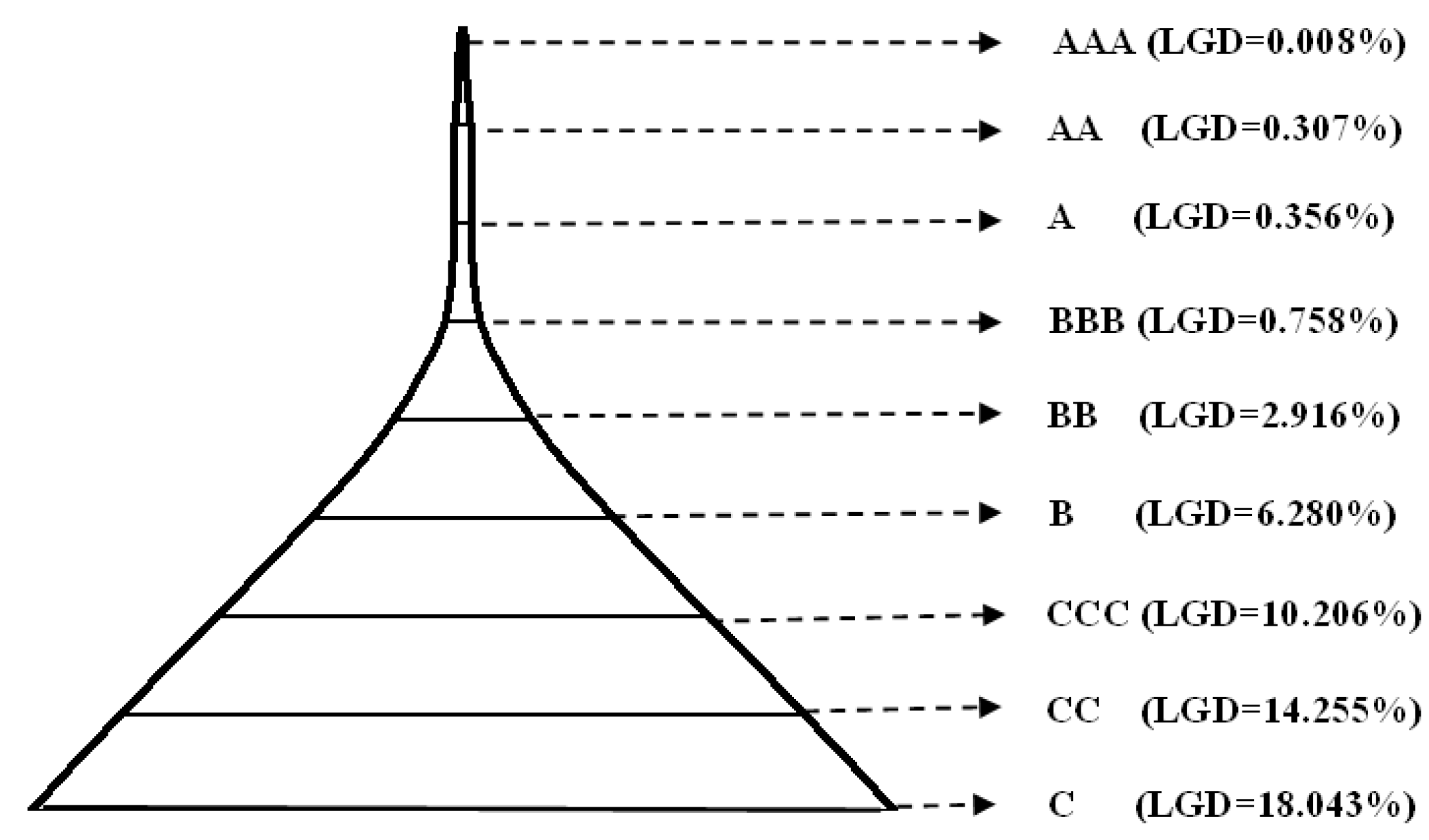
To better illustrate the default pyramid, we created a loss-given default distribution diagram based on the Loss Given Default rate LGD_k (see Figure 3). Figure 3 shows that the small enterprise credit rating classification model satisfies the pyramid principle such that higher credit ratings indicate lower rates of default and loss.

4. Conclusions

It is well known that the methods like Probit regression and stepwise regression have been successfully applied to credit rating for many years. However, the limited financial information and a small sample size of small enterprises looking for financing have leaded to a poor understanding of the general distribution of data. Moreover, the assumptions associated with general parametric models are difficult to satisfy in this domain. To make up the gap and help small enterprises get credit funds and help financial institutions select quality customers in the complex environment, we propose a model based on rank sum test and rank correlation analysis. We establish a credit rating system that clearly identifies the likelihood of defaults of small enterprises. The developed model is verified by the data of 1231 small enterprises.

The empirical analysis results are as follows. First, we discovered 22 indices capable of predicting small enterprise defaults, including main business revenue/cash ratio, gross margins, and number of contract breaches. Second, we weighted non-financial indices at 55%, showing that non-financial indices play a key role in identifying defaults among small enterprises. Third, the AUC value of the model is 0.863, showing that the credit rating model capable of discriminating defaults from non-defaults.

The contributions of the article are as follows. First, this is the first study that proposes a credit rating model for small enterprises by combining the approaches of the rank sum test and rank correlation analysis. Second, the proposed model predicts the credit rating of a new loan customer by utilizing the Z value capable of illustrating differences in ranks between the default sample and entire sample, which seems to offer new insight into the credit rating of customers.

Although we have introduced a novel credit rating approach, there is some room for further study. In this study, we have not compared this model with models based on Probit regression and stepwise regression, which will be done in the future as further research. In addition, there are also concerns about more relevant small enterprises data.

References

- State Administration for Industry & Commerce of the People’s Republic of China. Small Enterprise Development Report of China (Summary). Available online: http://www.saic.gov.cn/ywdt/gsyw/zjyw/xxb/201403/t20140331_143495.html (accessed on 20 December 2016).
- Wang, X. Non-Parametric Statistics; Renmin University of China Press: Beijing, China, 2005; pp. 120–181. [Google Scholar]
- Crook, J.N.; Edelman, D.B.; Thomas, L.C. Recent developments in consumer credit risk assessment. Eur. J. Oper. Res. 2007, 183, 1447–1465. [Google Scholar] [CrossRef]
- Myers, J.H.; Forgy, E.W. The Development of Numerical Credit Evaluation Systems. J. Am. Stat. Assoc. 1963, 58, 799–806. [Google Scholar] [CrossRef]
- Li, E.; Liu, L. Summary of Credit Evaluation Index System of Small and Micro enterprises. Credit Ref. 2013, 1, 67–70. [Google Scholar]
- Luo, P. Basel Committee on Banking Supervision, External Facility Ratings and Internal Facility Rating System; China Financial Publishing House: Beijing, China, 2004; pp. 9–10. [Google Scholar]
- Gumparthi, S.; Manickavasagam, V. Risk Classification Based on Discriminant Analysis for SME’. Int. J. Trade Econ. Financ. 2010, 1, 242–246. [Google Scholar] [CrossRef]
- Gumparthi, S.; Khatri, S.; Manickavasagam, V. Design and development of credit rating model for public sector banks in India: Special reference to small and medium enterprises. J. Account. Tax. 2011, 3, 105–124. [Google Scholar]
- Liu, C.; Wu, P.; Hao, D. Credit rating assessment study based on fuzzy set theory tech small and micro enterprises. Technol. Prog. Policy 2013, 30, 170–176. [Google Scholar]
- Fernandes, G.B.; Artes, R. Spatial dependence in credit risk and its improvement in credit scoring. Eur. J. Oper. Res. 2016, 249, 517–524. [Google Scholar] [CrossRef]
- Narain, B. Survival analysis and the credit granting decision. In Credit Scoring and Credit Control; Thomas, L.C., Crook, J.N., Edelman, D.B., Eds.; Oxford University Press: Oxford, UK, 1992; pp. 109–121. [Google Scholar]
- Cox, D.R. Regression Models and Life-Tables. J. R. Stat. Soc. 1972, 34, 187–220. [Google Scholar]
- Tong, E.N.C.; Mues, C.; Thomas, L.C. Mixture cure models in credit scoring: If and when borrowers default. Eur. J. Oper. Res. 2012, 218, 132–139. [Google Scholar] [CrossRef]
- Bellotti, T.; Crook, J. Support vector machines for credit scoring and discovery of significant features. Expert Syst. Appl. 2009, 36, 3302–3308. [Google Scholar] [CrossRef] [Green Version]
- Yu, L.; Yue, W.; Wang, S.; Lai, K.K. Support vector machine based multiagent ensemble learning for credit risk evaluation. Expert Syst. Appl. 2010, 37, 1351–1360. [Google Scholar] [CrossRef]
- Chen, N.; Vieira, A.; Ribeiro, B. A stable credit rating model based on learning vector quantization. Intell. Data Anal. 2011, 15, 237–250. [Google Scholar]
- Song, X.D.; Han, L.Y.D.; Han, L.Y. Credit Evaluation for Small-and-Medium-Sized-Enterprises Based on Fuzzy SVM with Dual Membership Values. Ind. Eng. 2012, 1, 93–98. [Google Scholar]
- Kim, K.J.; Ahn, H. A corporate credit rating model using multi-class support vector machines with an ordinal pairwise partitioning approach. Comput. Oper. Res. 2012, 39, 1800–1811. [Google Scholar] [CrossRef]
- Khashman, A. Credit risk evaluation using neural networks: Emotional versus conventional models. Appl. Soft Comput. J. 2011, 11, 5477–5484. [Google Scholar] [CrossRef]
- Hájek, P. Municipal credit rating modelling by neural networks. Decis. Support Syst. 2011, 51, 108–118. [Google Scholar] [CrossRef]
- Martens, D.; Baesens, B.; Gestel, T.V.; Vanthienen, J. Comprehensible credit scoring models using rule extraction from support vector machines. Eur. J. Oper. Res. 2008, 183, 1466–1476. [Google Scholar] [CrossRef]
- Yang, Y. Adaptive credit scoring with kernel learning methods. Eur. J. Oper. Res. 2007, 183, 1521–1536. [Google Scholar] [CrossRef]
- Wang, G.; Ma, J.; Huang, L.; Xu, K. Two credit scoring models based on dual strategy ensemble trees. Knowl.-Based Syst. 2012, 26, 61–68. [Google Scholar] [CrossRef]
- Kruppa, J.; Schwarz, A.; Arminger, G.; Ziegler, A. Consumer credit risk: Individual probability estimates using machine learning. Expert Syst. Appl. 2013, 40, 5125–5131. [Google Scholar] [CrossRef]
- Mandala, I.G.N.N.; Nawangpalupi, C.B.; Praktikto, F.R. Assessing credit risk: An application of data mining in a rural bank. Procedia Econ. Financ. 2012, 4, 406–412. [Google Scholar] [CrossRef]
- Yeh, C.C.; Lin, F.; Hsu, C.Y. A hybrid KMV model, random forests and rough set theory approach for credit rating. Knowl.-Based Syst. 2012, 33, 166–172. [Google Scholar] [CrossRef]
- Akkoç, S. An empirical comparison of conventional techniques, neural networks and the three stage hybrid Adaptive Neuro Fuzzy Inference System (ANFIS) model for credit scoring analysis: The case of Turkish credit card data. Eur. J. Oper. Res. 2012, 222, 168–178. [Google Scholar] [CrossRef]
- Van Gestel, T.; Baesens, B.; van Dijcke, P.; Suykens, J.A.K.; Garcia, J.; Alderweireld, T. Linear and non-linear credit scoring by combining logistic regression and support vector machines. J. Credit Risk 2005, 1, 31–60. [Google Scholar] [CrossRef]
- Zhang, H.; Mao, Z. Credit evaluation model based on the grey fuzzy and the multidimensional time series. J. Manag. Sci. China 2011, 14, 28–37. [Google Scholar]
- Florez-Lopez, R. Modelling of insurers’ rating determinants. An application of machine learning techniques and statistical models. Eur. J. Oper. Res. 2007, 183, 1488–1512. [Google Scholar] [CrossRef]
- Finlay, S. Multiple classifier architectures and their application to credit risk assessment. Eur. J. Oper. Res. 2011, 210, 368–378. [Google Scholar] [CrossRef]
- Paleologo, G.; Elisseeff, A.; Antonini, G. Subagging for credit scoring models. Eur. J. Oper. Res. 2010, 201, 490–499. [Google Scholar] [CrossRef]
- Shi, B.; Yang, H.; Wang, J.; Zhao, J. City green economy evaluation: Empirical evidence from 15 sub-provincial cities in China. Sustainability 2016, 8, 551. [Google Scholar] [CrossRef]
- Shi, B.; Chen, N.; Wang, J. A credit rating model of microfinance based on fuzzy cluster analysis and fuzzy pattern recognition: Empirical evidence from Chinese 2,157 small private businesses. J. Intell. Fuzzy Syst. 2016, 31, 3095–3102. [Google Scholar] [CrossRef]
- Zhou, Q.; Tian, P.; Tian, Z. Estimation of non-normal process capability index based on johnson system of transformations. Syst. Eng. 2004, 05, 98–102. [Google Scholar]
- Shapiro, S.S.; Wilk, M.B. An Analysis of Variance Test for Normality (Complete Samples). Technometrics 1965, 52, 591–611. [Google Scholar]
- Yang, W.; Qiao, J. Use of Mann-Whitney U-test in Analysis on Selection of Avian Habitats. Arid Zone Res. 2001, 18, 42–44. Available online: http://d.wanfangdata.com.cn/Periodical/ghqyj200103008 (accessed on 11 October 2017). (In Chinese).
- Hu, J.; Kong, H.; Li, Y. Reliability and validity evaluation on the health literacy questionnaire of priority in fectious diseases prevention for priority populations in China. Chin. Health Educ. 2011, 27, 282–284. [Google Scholar]
- Zhang, S.; Zhang, M.; Chi, G. The Science and Technology Evaluation Model Based on Entropy Weight and Empirical Research During the 10th Five-Year of China. Chin. J. Manag. 2011, 7, 34–42. [Google Scholar]
- Shi, B.; Meng, B.; Wang, J. An Optimal Decision Assessment Model Based on the Acceptable Maximum LGD of Commercial Banks and Its Application. Sci. Program. 2016. [Google Scholar] [CrossRef]
- Chi, G.; Cheng, Y. Based on Credit Rating and Default Loss Rate of Matching and Method of Credit Rating System. Chinese Patent ZL201210201114.3, 16 September 2015. [Google Scholar]
- Ministry of Industry and Information Technology; National Bureau of Statistics; National Development and Reform Commission; Ministry of Finance. Standard Type Division for Middle and Small-Sized Enterprises. Available online: http://www.gov.cn/zwgk/2011-07/04/content_1898747.htm (accessed on 10 May 2017).
- Terdpaopong, K.; Mihret, D.G. Modelling SME credit risk: Thai empirical evidence. Small Enterp. Res. 2011, 18, 63–79. [Google Scholar] [CrossRef]
- Wang, C.; Li, W. Credit Risk Assessment in Commercial Banks: Projection Pursuit Discriminant Model. J. Ind. Eng./Eng. Manag. 2000, 14, 43–46. Available online: http://d.wanfangdata.com.cn/Periodical/glgcxb200002013 (accessed on 11 October 2017). (In Chinese).
Figure 1.
The conceptual model of the small enterprise credit rating model.
Figure 2.
The ROC curve of the credit rating model.
Figure 3.
The LGD distribution of small enterprise credit ratings.