Temperature Control by Its Forecasting Applying Score Fusion for Sustainable Development

Abstract

Temperature control and its prediction has turned into a research challenge for the knowledge of the planet and its effects on different human activities and this will assure, in conjunction with energy efficiency, a sustainable development reducing CO₂ emissions and fuel consumption. This work tries to offer a practical solution to temperature forecast and control, which has been traditionally carried out by specialized institutes. For the accomplishment of temperature estimation, a score fusion block based on Artificial Neural Networks was used. The dataset is composed by data from a meteorological station, using 20,000 temperature values and 10,000 samples of several meteorological parameters. Thus, the complexity of the traditional forecasting models is resolved. As a result, a practical system has been obtained, reaching a mean squared error of 0.136 °C for short period of time prediction and 5 °C for large period of time prediction.

1. Introduction

Modern societies are conditioned by many natural factors, such as, for example, the weather. The meteorological changes affect to different aspects of our lives. These changes not only have influence over the fields which are more directly connected with climatology, as the agricultural sector, but also over others which are more complex and apparently dissociated from atmospheric reality, as energy efficiency, and this becomes in an important factor in planning for sustainable urban development.

In fact, the climate is an important factor that affects the economy. It is especially important, not only in areas based on systems of agricultural production (such as developing countries) but also in other areas technologically developed and whose economies are based on other sectors such as tourism, or even in those that try to approach a sustainable economy through renewable energy sources [1]. Prediction is, therefore, a tool to be modelled and developed that can be compared to different procedures from each specific area. There are currently three important trends which tackle this theme: Climatology, acting as empirical tradition; Physics of the Atmosphere, as theoretical tradition; or Numerical Weather Prediction (NWP), as modern tradition [2]. These recent mathematical models struggle at present to achieve a shorter response time as main target. However, the more accurate the method is, the more data is required and therefore a longer response time is obtained.

Meteorological services hold that the solution to that problem lies in the development of traditional computing algorithms but in fact, there are emerging alternatives focused on the future of weather forecast, such as Artificial Neural Networks (ANN) with supervised learning. Temperature prediction through time series is an important technique, in which past observations of certain weather variables are collected and analyzed to develop a model based on the underlying relationship between them. It is important to have in mind that any temperature modeling is a chaotic system in which small errors in the initial prediction conditions grow very quickly and affect the predictability [3].

Mathematical models based on linear methods have been used for prediction of time series but the appearance of Artificial Neural Networks have offered a possibility to set new methodologies. These ANN models are at present acquiring a great relevance for the recognition of patterns and even for the biometrics. In the last decades some related works on meteorology have been developed, for example, in an approach to the coexistence of these models, G. Peter Zhang [4] proposed in 2001 a hybrid system using the linear method ARIMA (Auto Regressive Integrated Moving Average) and ANNs at the same time. In this study, it was concluded that the nonlinear model of ANN offers results which are slightly more favorable against the complexity of the linear system, because the most important advantage of ANN is their flexible nonlinear modeling potential.

In the field of meteorology, ANNs are also being used for prediction of atmospheric phenomena and its application to power generation systems. In 2007, Sorjamaa, Hao, Reyhani, Ji and Lendasse [5] proposed a global methodology for the long-term prediction of time series, combining direct prediction strategy and sophisticated input selection criteria. This methodology was successfully applied to the Poland Electricity Load dataset.

In 2009, Ellouz, Ben-Jmaa-Derbel and Kanoun [6] used ANNs to propose a tool to be able to evaluate aspects of the heat interchange between land and air through underground pipes in order to achieve improvements in weather conditions of the building, with a prediction error between the predicted and the experimental outlet temperature of 1.1 °C from 8 pm to 8 am and an error lower than 4 °C from 10 am to 5 pm. A year later, Fan, Methaprayoon and Lee [7] made overload forecasting considering meteorological predictions. The results were very positive and it helped to improve the energy efficiency of the power station at precise times of higher electricity demand, obtaining an error of 2 °C. In 2011, Rastogi, Srivastava, Srivastava and Pandey [8] used patterns analysis with ANNs for temperature forecasting. With those results, the efficiency of the proposed model was demonstrated with a high accuracy between actual values and predicted values. In the same year, Chen and Xu [9] implemented a model based on ANNs for the prediction of temperature and humidity roadways of coal mines. The results had an error range, which was within the limits fixed (0.2% to 4.9%). Afterwards, in Bangladesh (2012), Routh, Bin Yousuf, Hossain, Asasduzzaman, Hossain, Husnaeen and Mubarak [10] also performed temperature predictions using models based on ANNs to improve energy efficiency in solar power stations. In this last case the results were also favorable. A little later (2013), Huang, Chen, Mohammadzaheri, Hu and Chen [11] also used these models to make a multi-zone temperature prediction in the terminal building of the airport of Australia, where the results achieved a prediction error of just 1 °C.

Taking into account the diversity and progress in prediction strategies for multi-step ahead prediction, Ben Taieb, Bontempi, Atiya and Sorjamaa [12] made in 2012 a review of the different existing strategies for multi-step ahead forecasting and made a comparison between them, in theoretical and practical terms. As a conclusion they observed that the complexity of making a forecast of time series many steps into the future is high due to the uncertainty, which increases with a larger time horizon.

Using data from the same meteorological stations of this research, Vásquez, Travieso, Pérez, Alonso y Briceño [13] presented a system that reaches an error of 0.28 °C making temperature predictions using multilayer ANN.

In 2013, Xiong, Bao and Hu [14] proposed a revised hybrid model built upon empirical mode decomposition based on the feed-forward neural network modeling framework incorporating the slope based method. The model was applied to obtain a prediction of crude oil prices, obtaining great accuracy. In 2014, Hernández-Travieso, Travieso and Alonso [15] also used ANNs to predict wind speed using data from meteorological stations situated in Gran Canaria and Tenerife (Canary Islands, Spain). In this work, ANN proved to be a powerful tool to make an accurate prediction obtaining a mean absolute error (MAE) of 0.85 meters per second. In 2014, Bao, Xiong and Hu [16] proposed a particle swarm optimization based multiple-input several multiple-outputs (PSO-MISMO) modeling strategy, having the capability to determine the number of sub-models in a self-adaptive mode, with variable predictions. The strategy has been validated with simulated and real datasets. In 2015, Li, Qin, Ma and Wu [17] used ANN to make a prediction of greenhouse inside temperature in the typical summer climate in China, reaching a mean square error of 0.01 °C. In addition, in 2015, McKinney, Pallipuram, Vargas, Taufer [18], made a research to study extreme climate events, and unusually high and low temperatures were studied on it. They reach results of more than 90% hits. In 2016, Prashanthi, Meganathan, Krishnan, Varahasamy, Swaminathan [19] proposed a model that finds the extreme hot day prediction 24 and 48 h ahead with the help of local weather parameters.

The importance of temperature and sea level rise is shown by Aral and Guan [20] in 2016, where the impact of sea surface temperature and sea levels in previous years is included on current sea level rise. There is a relationship between temperature and sea level rise. The same conclusion was reached by Arora and Dash [21] in 2016, the sea-air temperature contrast also contributes to fuels tropical cyclone systems increasing its destructive power.

All there are examples that highlights the importance of an accurate temperature prediction, not only to reduce CO₂ emissions, which is especially important in urban areas, but also to serve as a tool to aid emergency systems in order to be able to be one step ahead of natural disasters.

Therefore, although temperature forecasting is a very complex and imprecise science, these studies have shown that ANNs have a powerful capability of classification and pattern recognition and can be used as tools to achieve accurate predictions in the field of meteorology [22].

In this research, four contributions or innovations versus the state-of-the-art are proposed. First of all, the feedback topology was used to study different configurations, in order to determine how the behavior of this architecture for using in temperature forecasting is. Secondly, a combined input-stimulus with information from other meteorological parameters, which directly affect daily cycles of temperature, is presented. Thirdly, an optimization based on a score fusion method has been introduced to evaluate heuristically whether it improves the degree of forecasting of this proposal. Finally, a standardization of input-data in the system was also established, that will impact positively during the training phase.

In this research, a system based in a backpropagation-ANN using Score Fusion is proposed for temperature forecast. To do this, information from real meteorological stations is taken for the prediction. The model will be tested using non-feedback topology to get immediate predictions but also using feedback topology to obtain long-term predictions. This last distinguishing aspect will make it possible to reach new contributions to the scientific community since ANNs that respond in a feedback architecture, have not been previously studied in detail. The flow chart of Figure 1 summarizes the main steps developed in the proposed model.

The remainder of this paper is as follows. In Section 2, theoretical aspects of the backpropagation ANNs using Score Fusion will be briefly discussed, as well as the decisions which have been taken in the design of this proposed model. Afterwards, the results obtained during the different experiments will be exposed in Section 3. Section 4 presents the discussion of the results obtained and the comparison with previous works. Finally, in Section 5, the conclusions of this research will be presented.

2. Materials and Methods

After studying previous works for time series forecasting in the state-of-the-art, a backpropagation topology has been used for the development and implementation of this research, showing an improvement versus the ANN model only when Score Fusion is used. Models based in backpropagation-ANN [4] are the most appropriate architecture to estimate future values from training with time series against any other topologies or even against conventional linear methods, due to the adaptability of the system.

Artificial Neural Networks are an information processing paradigm which is inspired by the biological nervous systems. The key element of this paradigm is the new structure of the information processing system. It is composed of a large number of highly interconnected processing elements (neurons), working together to solve specific problems. A neural network is a powerful data modeling tool that is able to capture and represent complex input-output relationships [23]. One of its types, Multilayer ANN, is a network consisting of multiple layers of action and for the proposed model it will consist of three layers. The first one, input layer, receives information from external sources. The second one, hidden layer, is responsible for running the internal processes of the network. The third one, performance or output layer is responsible for communicating the response of the system to the outside.

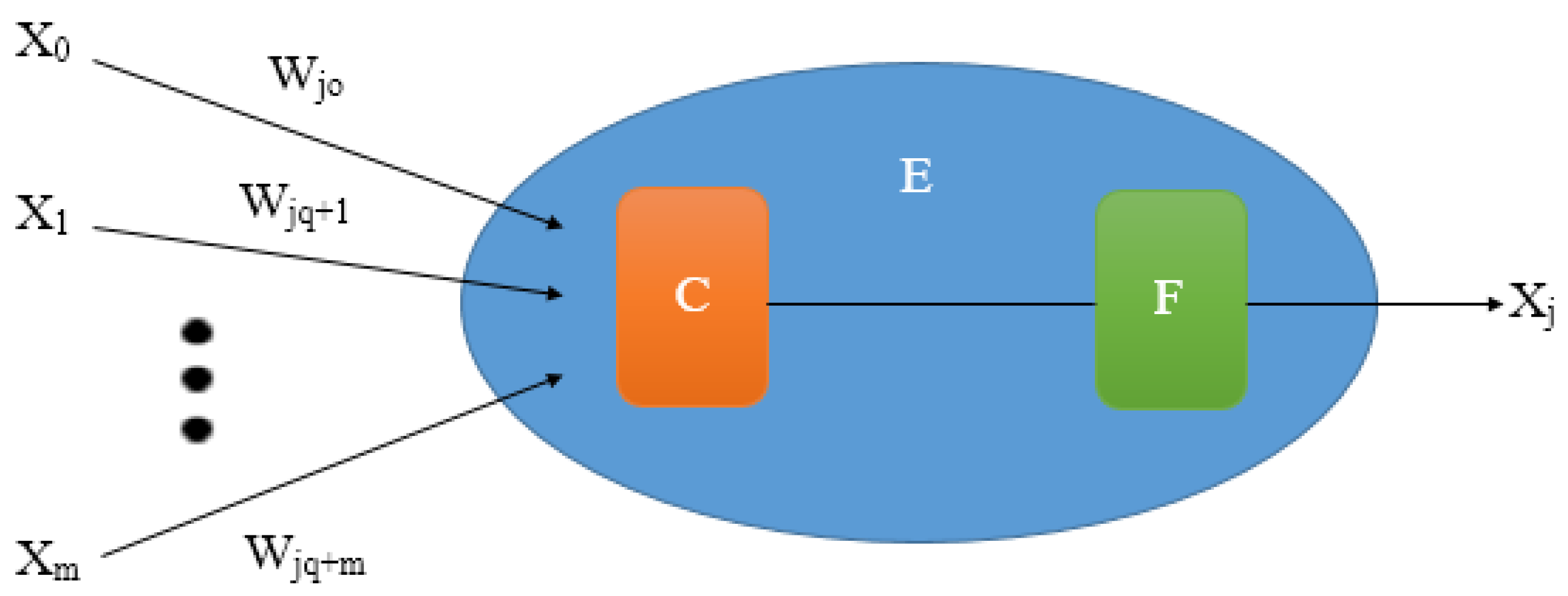
Each one of these layers is comprised of elementary processing units which are called artificial neurons. Each neuron has individually a certain number of entries, a processing node and a single output and each connection between neurons is associated with a weight value [24]. ANNs are able to model the relationship between inputs and outputs by modifying the weight values of the connections. Therefore, an ANN is configured for a particular application, such as pattern recognition or data classification, through a learning process. For this research, the Backpropagation Method was used, which is characterized by a supervised learning type. A diagram of an artificial neuron is shown on Figure 2; where Wji is the weight associated to each input-Xi of the j-neuron. In addition, this neuron is formed by a combination function C (which adds input-signals), an Operational Element E (associated to the weight value) and an Activation Function F.

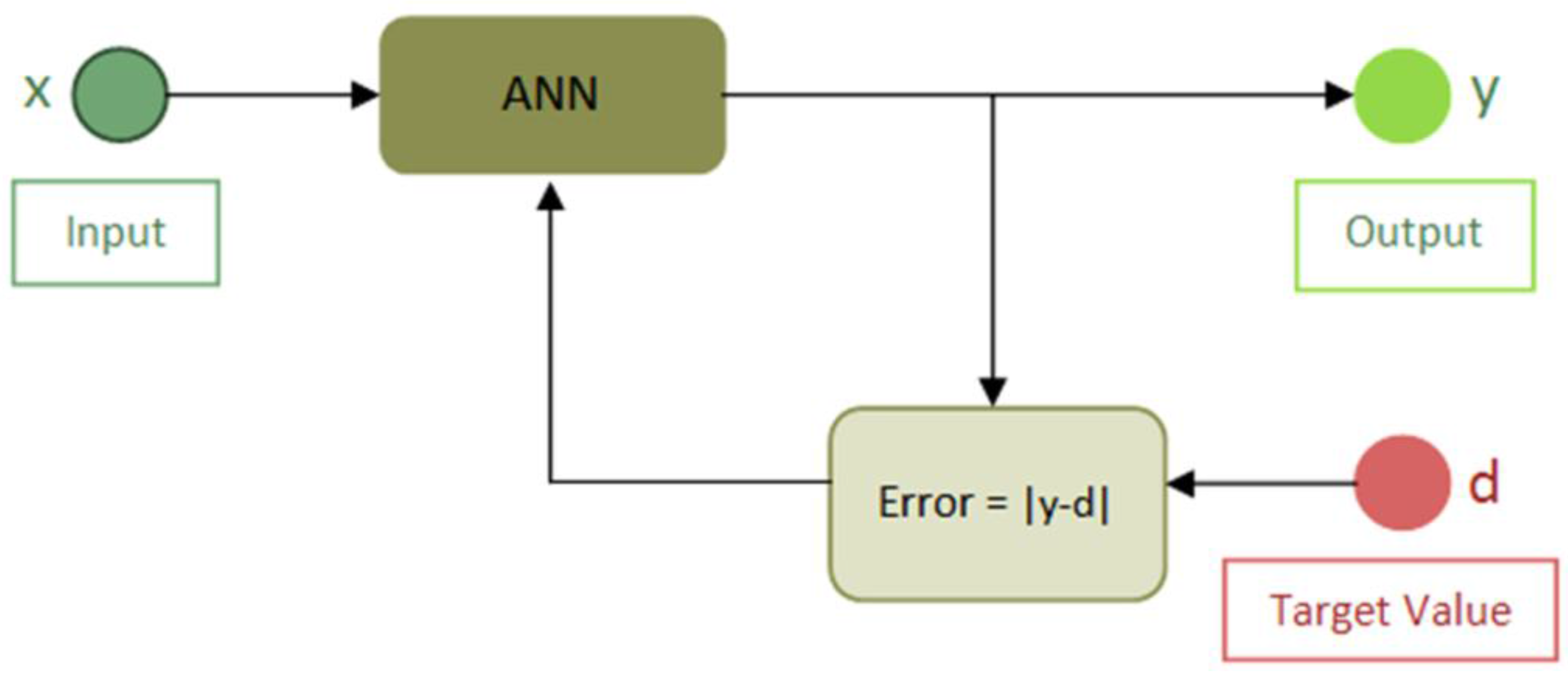
Backpropagation is commonly used as a training method in conjunction with an optimization approach such as gradient descent (based on Steepest Descent method) and it shows results closed to real values (MAE = 0.136 °C for predictions within hours). This method calculates the gradient of a loss function according to all the weights in the network. The resulted gradient is fed back to the optimization method which, in turns, uses it to update the weights in an attempt to minimize the loss function. This Backpropagation algorithm is made up of two phases: a forward phase and a backward phase. In the forward phase, the activations are propagated from the input (x) to the output layer. In the backward phase, the error between the observed actual value (target d) and the requested nominal value (y) in the output layer is propagated backwards in order to modify the internal weight values (W_ji) of the network, as shown in Figure 3. It is important to note that, generally, the initialization of these weight values (W_ji) has been done randomly. Once the ANN reaches the training convergence, the experiment proceeds to the next stage for prediction where the Score Fusion module was applied.

To perform this proposed method, a database from a village in the Republic of Costa Rica has been used. This locality, called Turrialba, is an interesting place characterized by a climate of contrasts. Turrialba is surrounded by a river and emplaced on slopes of a currently active volcano which affects directly the climate of the area.

The original database for this research is presented in Excel format, containing various meteorological variables such as temperature, humidity, atmospheric pressure, wind speed, etc. The data was obtained between July 2007 and September 2008 and presents a sampling frequency of 30 min. This last aspect is very important to note because the use of lower sampling frequencies could generate unfavorable results in future works.

At the preprocessing stage, to choose the elements involved in combined input-stimulus, the most influential meteorological elements on daily cycles of temperature have been studied. Depending on the limitations of meteorological database, solar radiation, leaf wetness and time of sample acquisition have been chosen [25,26]; where “leaf wetness” is the quantity of condensed water-vapor on the plant leaves. It indicates the humidity and measures the electrical resistance which the plant has from the humid environment. When the relative humidity is high, the electrical resistance is low, and the leaf wetness is low. The “time of sample acquisition” value refers to the time when the meteorological station acquires the meteorological parameter. Later, normalization of input-data values between (−1, 1) was established in order to solve two problems. Firstly, data dispersion presented by working with parameters from different scales of measurement is clearly reduced. Secondly, the range of values taken by the weight values of neurons is bounded, achieving a faster and more stable convergence during the training phase.

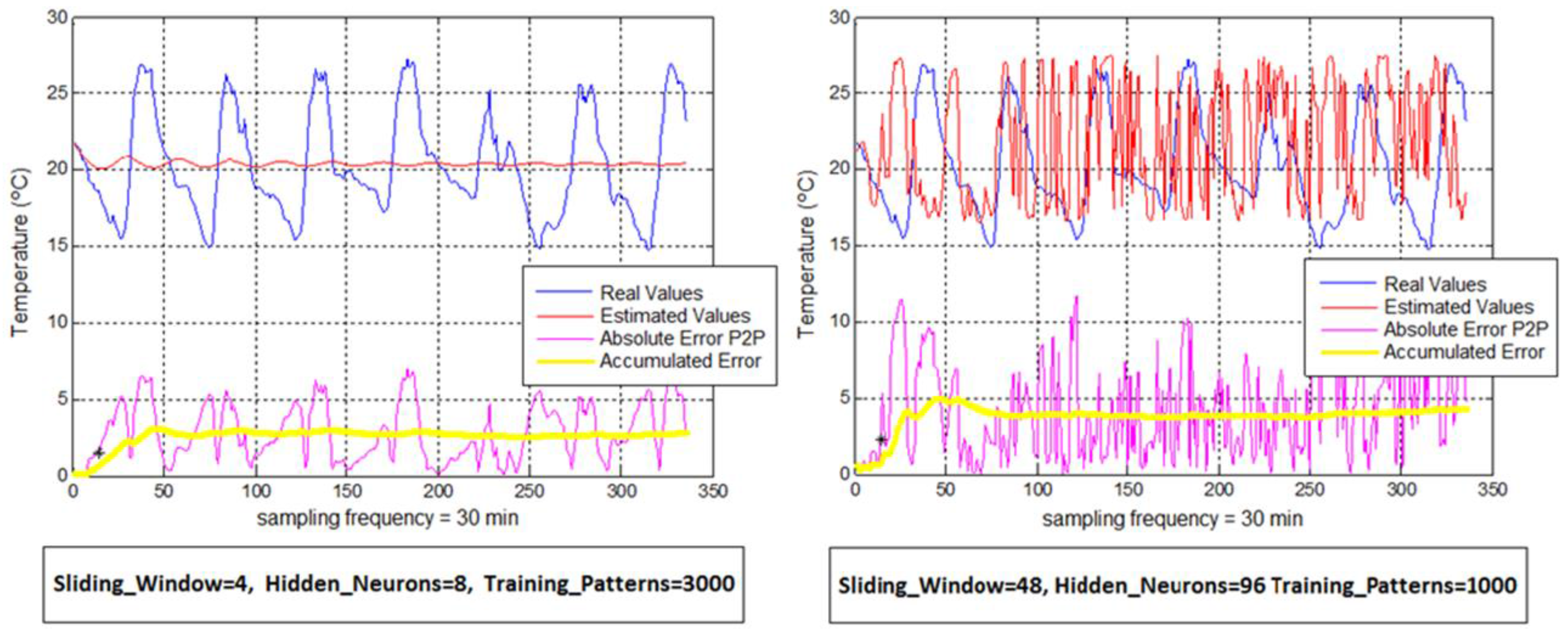
Regarding the configuration of the proposed system, it is set based on three parameters. Firstly, the window length, which represents the sliding window in time to capture values from the database, determines the number of neurons in the input layer. This sliding window represents the number of past values needed to obtain a temperature prediction. Secondly, the number of neurons in the hidden layer, which defines the number of fixed neurons for the middle layer and finally, the number of training patterns, which represents the quantity of examples offered to the ANN for the training stage. Thirdly, different settings will be established with the benchmarks to study the response of the model.

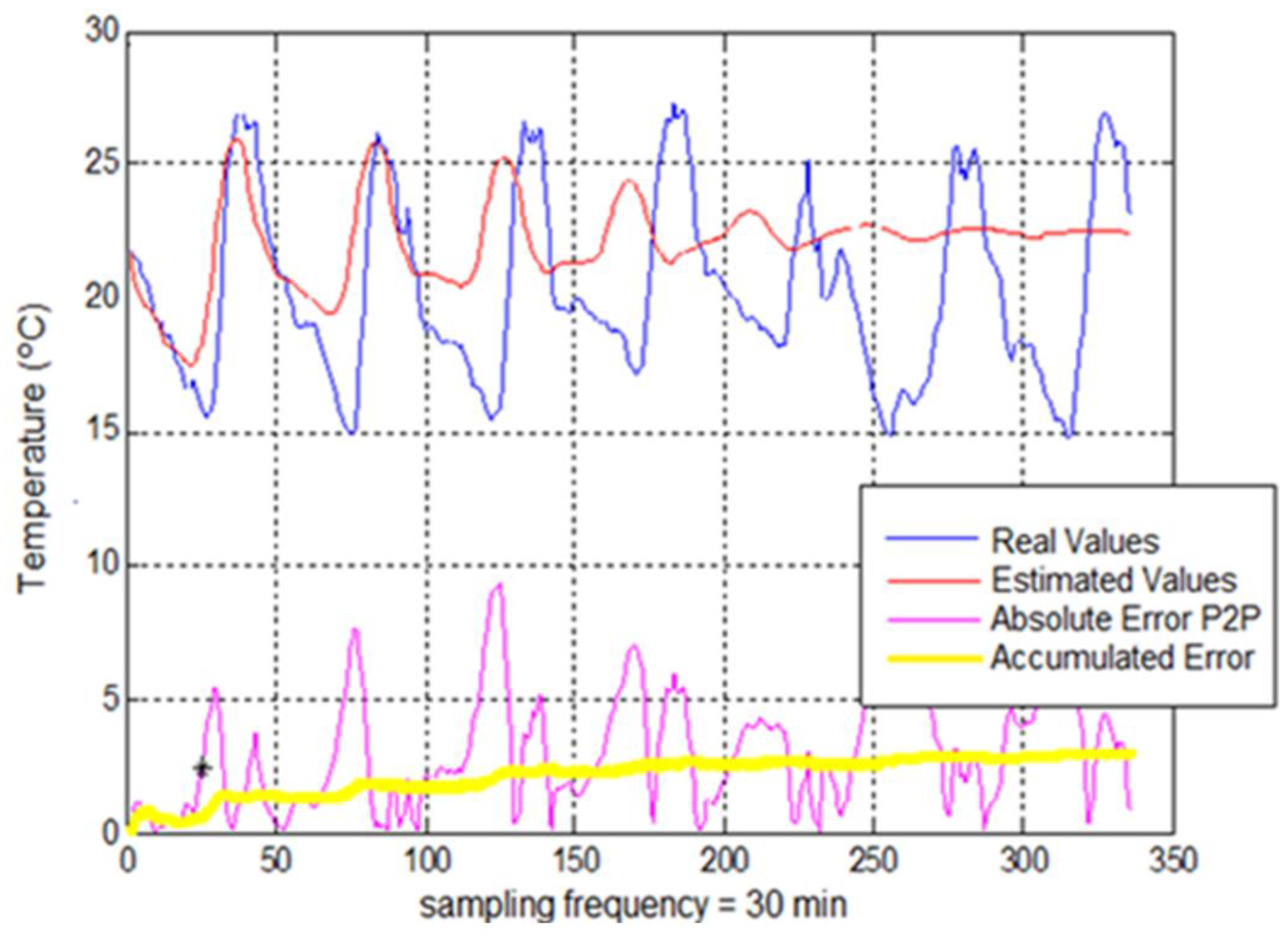
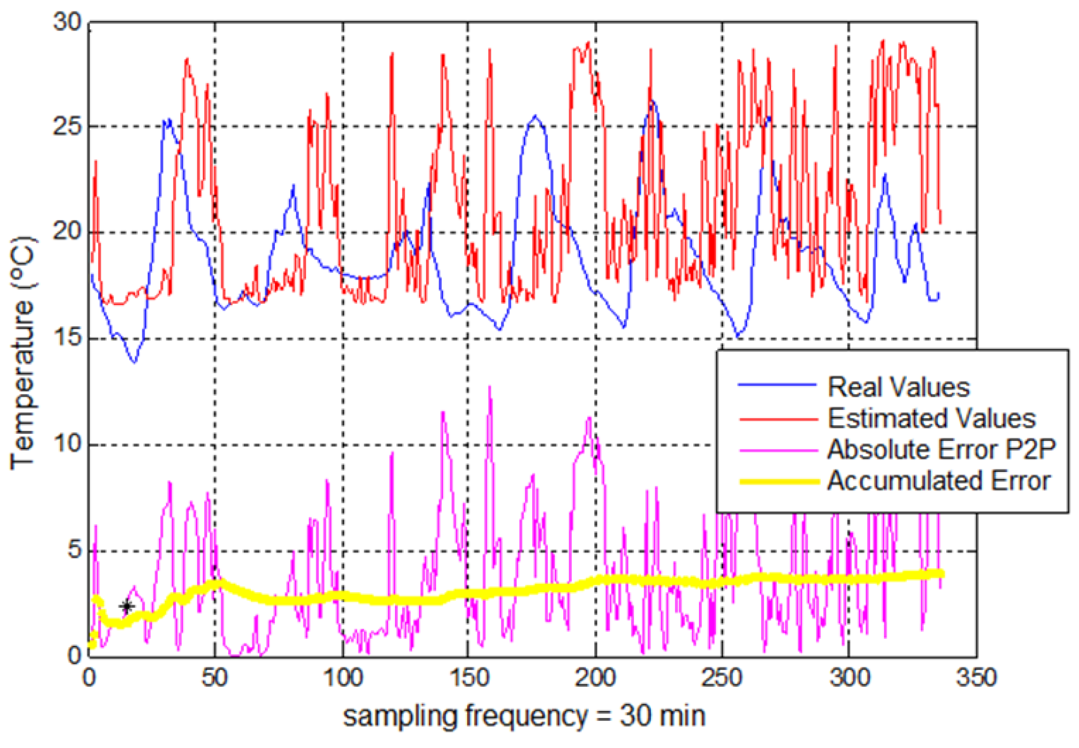
It offers two clearly differentiated working modes. The first one will be characterized by a non-feedback topology to get values of immediate prediction, where each sliding window formed by real values will estimate a single value of temperature. The second one will be characterized by a feedback topology to get short-term predictions, where, from a single window, a continuous prediction in time will run using estimated values to generate new temperature values.

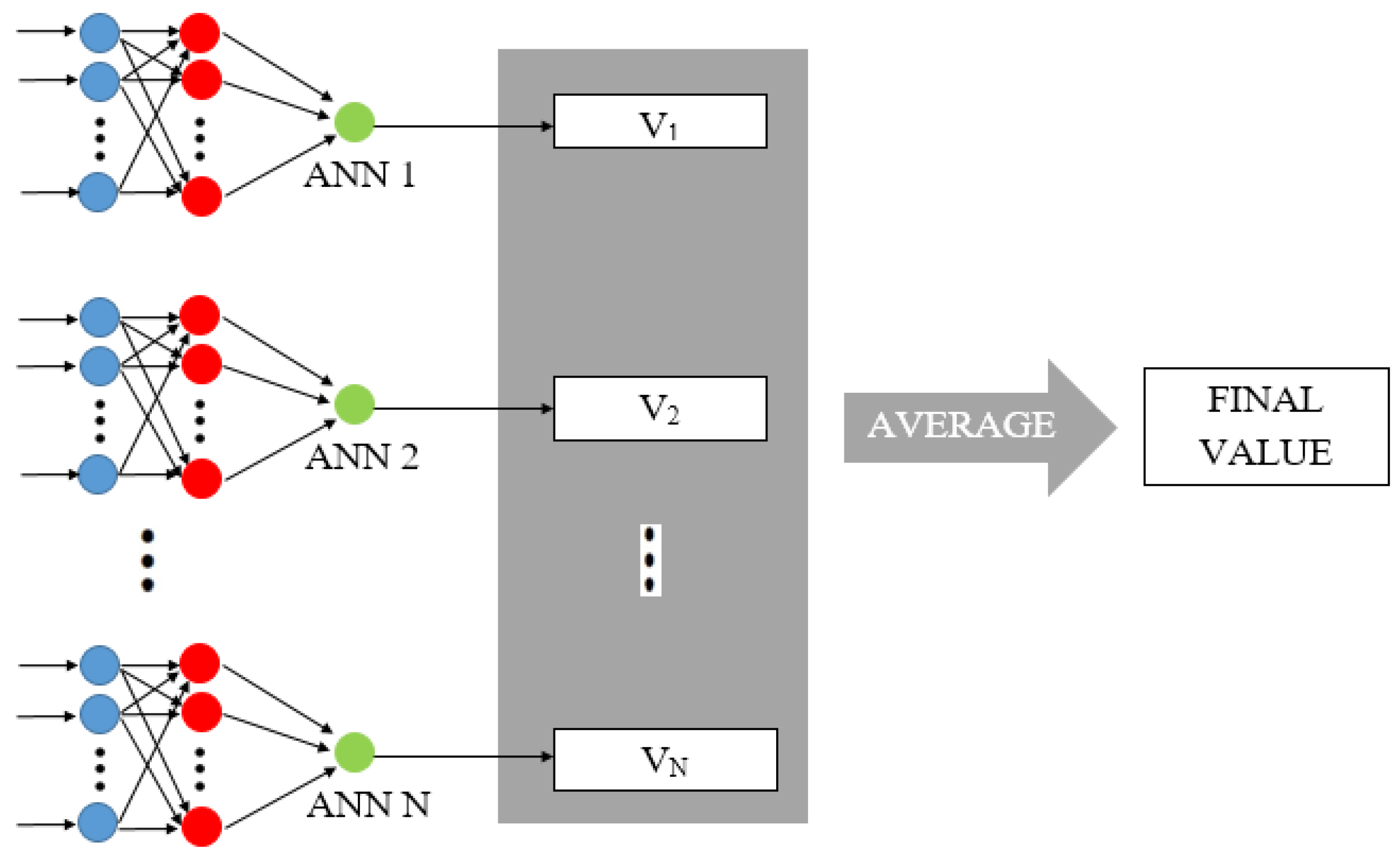
The last step of our process, Score Fusion, specifically the technique of Adding-Score has been introduced to evaluate whether or not it is effective in improving the degree of forecast for the proposed model. In this case, a backpropagation architecture that generates a random initialization of weight values is used. This fact causes that two ANNs, which have been equally configured and trained with the same training patterns; generate different responses due to the random initialization of the ANN weights. These responses are very similar, but not exactly the same. In this way, the optimization method is conceived as a neural structure consisting of several identical ANNs working in parallel. The overall response, represented by Equation (1), corresponds to the calculation of the average value of all the ANNs (see Figure 4).

$$Final Value=\frac{1}{N} {\displaystyle \sum }_{i=1}^N{V}_i$$

(1)

Since the ANN is modelled to maximize the success rate, this ANN is applied multiple times in parallel using random initialization. As shown in Figure 4, Adding-Score is formed by a set of “N” ANN in parallel and where the final value is calculated as the average of responses of each ANNi.

Independently of this topology, the system will be stimulated with observations of different nature. On the one hand, it will be stimulated by only temperature values to get estimations of this variable. On the other hand, a combined input-stimulus with other meteorological elements will be used together with the temperature data to get predicted temperature values, so it can be studied whether using multiple input-information which improves the level of each prediction. In this way, four different working modes can be well defined. For an easy explanation of results achieved during the stage of experimentation, the following nomenclature has been proposed to define each mode in

Table 1. Working modes and their definition.

Working Mode	Single Input-Stimulus	Combined Input-Stimulus
Non-feedback topology (Immediate Prediction)	MODE.1	MODE.2
Feedback topology (Short-Term Prediction)	MODE.3	MODE.4; MODE.4v2

.

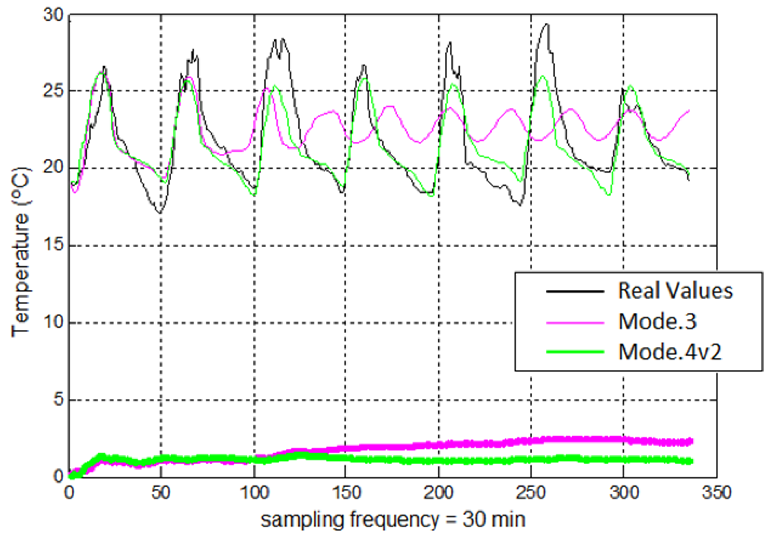
For modes that make use of temperature values (Mode.1 and Mode.3), a dataset of 20,000 samples have been used, whereas for the others (Mode.2, Mode.4 and Mode.4v2) a dataset of 10,000 samples was selected. The difference in the number of samples is due to the fact that the best results are obtained with these parameters. The difference between Mode.4 and Mode.4v2 is that in Mode.4v2 the sampling time parameter is also used in the prediction.

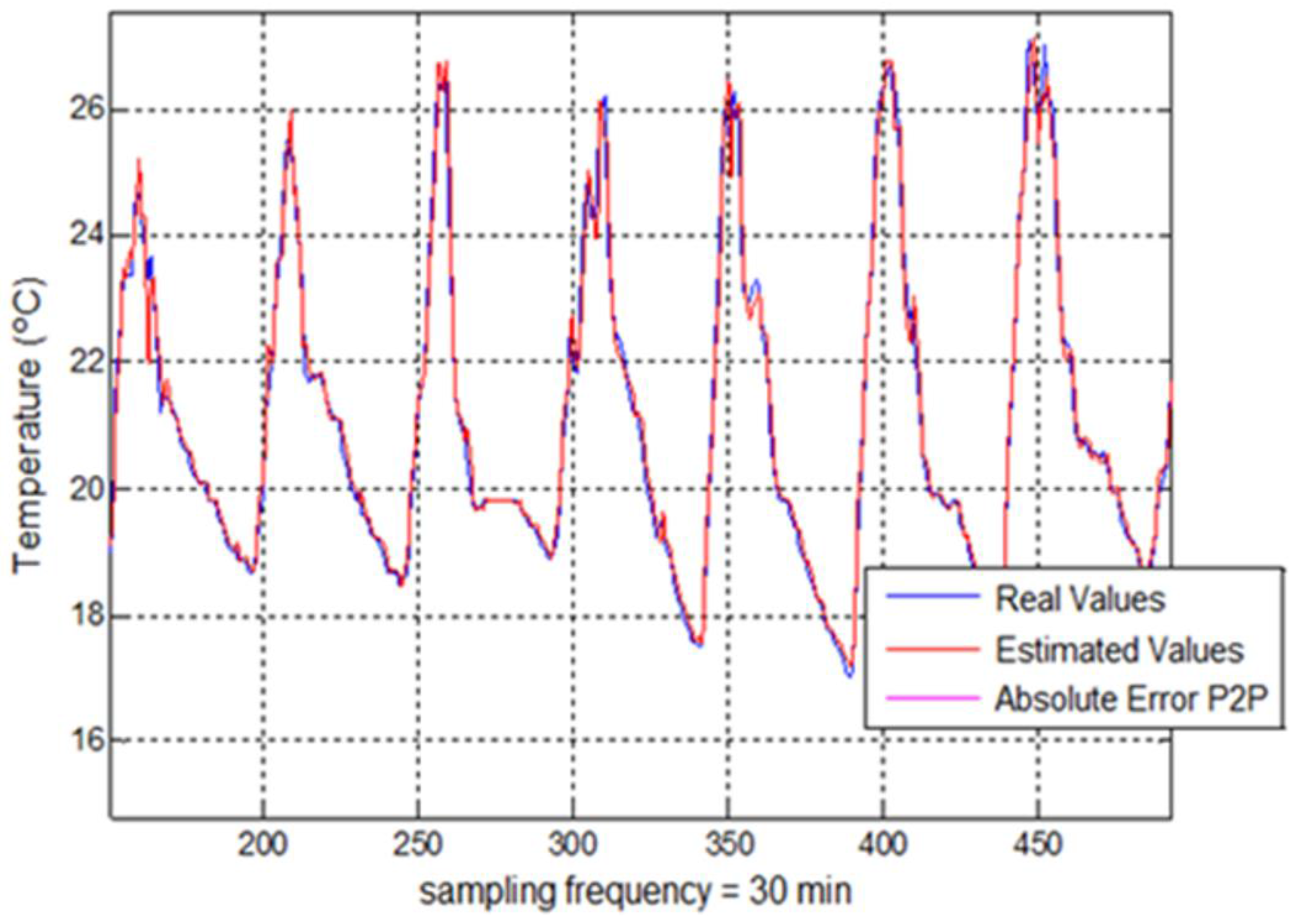
Regarding the evaluation of error parameters, two goodness criteria have been established according to both topologies. Thus, for the non-feedback topology, mean absolute error (MAE) parameter was proposed as an indicator for a dataset of estimated values whereas for the feedback topology, it was set up mainly the accumulated error parameter, which determines the evolution of the absolute error for each new estimated temperature value and it is defined as the absolute error of the use of estimated samples to estimate future predictions (estimated samples for a feedback mode).

In order to improve the efficiency of our classification system, a Score Fusion module was applied. The goal of this module was to reduce the effect introduced by the random initial of the weights used in the neural networks. Using “N” neural networks, obtaining “N” different solutions for the same input data. The idea was to amalgamate the “N” outputs in order to generalize the output to the results of neural networks that perform better.

Score Fusion is the name used to refer to the different mathematical methods for obtaining a better result once the experiment is done. That means that, when the ANN shows its results, it is possible to improve with some mathematical operations. In our case, the Score Fusion technique used is Adding-Score. This specific technique is based on the addition of mono-modal scores reached by each ANN during the experiment. This fusion block is applied based on the random initialization of weights and different convergences reached each time that an ANN is executed. Therefore, to establish a generalization, but always applying the same input data [27], “N” ANN are executed and theirs outputs are fused using Adding-Score.

3. Results

In this section, once the experiments described in Table 1 are realized, the best results for each mode of running are presented. They have been obtained by diverse benchmarks tests, in which the ANN has been subjected to different configurations by modifying the sliding window, the number of hidden neurons and the number of training patterns parameters. Moreover, an optimization based on Adding-Score approach has been applied for each optimal result in order to reduce the error rate of the proposed model.

For each of the modes described in Table 1, a set of configurations were used to experiment with overall simulations to determine the best results. After locating the best configurations, they have been again simulated in order to establish which configuration was more efficient. Subsequently, each parameter was varied with values close to the optimal configuration to see if new enhancements were achieved in the system response. Finally, some of the results, including the best results for each mode, as well as others that are representative, are presented in this paper.

3.1. Mode.1

For Mode.1, the overall simulation was established with the combination of the parameter values showed in

Table 2. Used parameter values for the overall simulation in Mode.1.

Type of Mode	Sliding Window Length	Hidden Neurons	Training Patterns
MODE.1	4, 5, 6, 12, 24, 36, 48	8, 12, 16, 24, 32, 64	1000, 3000, 5000, 8000

.

Table 3. Best result in Mode.1.

Setting	Sliding Window Length	4
	Hidden Neurons	12
	Training Patterns	3000
Mean Absolute Error	0.2639 °C
Mean Squared Error	0.1659 °C
Training Time	35.33 s
Simulation times	3.96 × 10−2 s

presents the selected best result for Mode.1. It has been obtained for the described configuration where the MAE rate did not exceed the value of 0.2639 °C for a dataset of 1000 simulated samples. In Figure 5, can be also seen how estimates generated by the system are closely suited to the daily cycles of real temperature.

After executing the Adding-Score, it has been verified that this optimization slightly improves the degree of forecast but only for a few hundredths of Celsius degree. For this reason, the results will be indicated with four decimals in the followings tables. Thus, it is important to evaluate whether this improvement reaches the required needs for the intended purpose.

Table 4. Results obtained for different numbers of ANNs in parallel for Adding-Score (Mode.1 Test1).

Adding-Score (Mode.1 Test1)	N = 1	N = 5	N = 10	N = 15
MAE (°C)	0.2770	0.2701	0.2681	0.2692

N represents the number of ANNs in parallel used on several benchmarks test.

and

Table 5. Results obtained for different numbers of ANNs in parallel for Adding-Score (Mode.1 Test5).

Adding-Score (Mode.1 Test5)	N = 1	N = 5	N = 10	N = 15
MAE (°C)	0.3450	0.3361	0.3352	0.3340

N represents the number of ANNs in parallel used on several benchmarks test.

shows the results obtained for MAE and various settings of the Adding-Score method running in Mode.1, where N represents the number of ANNs in parallel used on several benchmarks test varying it in order to obtain best results (when N = 1, the first random ANN was used).

Although the improvement of 15 ANN with comparison to 1 ANN is marginal, our latency time is 1 h, so we have enough time to train again the system. This means that, it is not convenient to the execution with 15 ANN.

3.2. Mode.2

For Mode.2, the overall simulation was established with the combination of the parameters shown in

Table 6. Used parameter values for the overall simulation in Mode.2.

Type of Mode	Sliding Window Length	Hidden Neurons	Training Patterns
MODE.2	4, 6, 12, 24, 36, 48	8, 12, 16, 24, 32	1000, 3000, 4000, 5000

.

The best results for Mode.2 are shown in

Table 7. Best result in Mode.2.

Setting	Sliding Window Length	4
	Hidden Neurons	8
	Training Patterns	4000
Mean Absolute Error	0.2294 °C
Mean Squared Error	0.1359 °C
Training Time	52.94 s
Simulation times	4.04 × 10−2 s

, where the MAE rate did not exceed the value of 0.2294 °C for a dataset of 1000 simulated samples. Therefore, it is confirmed that the use of combined input-stimulus improves the forecast reducing MAE by 15%, approximately, compared to Mode.1. Paying attention to Figure 6, it can be equally noticed how generated estimates are also closely suited to the daily cycles of real temperature. Moreover, it is important to note how the number of required hidden neurons is lower than in the previous mode.

As far as optimization based on Adding-Score approach is concerned, similar aspects are concluded for this mode. It is also interesting to note, once the experiments were carried out, how for systems which are composed of more than 5 ANNs, their responses are often worse than for a single ANN (see

Table 8. Results obtained for different numbers of ANNs in parallel for Adding-Score (Mode.2 Test1).

Adding-Score (Mode.2 Test1)	N = 1	N = 5	N = 10	N = 15
MAE (°C)	0.2804	0.2754	0.2857	0.2832

N represents the number of ANNs in parallel used on several benchmarks test.

and

Table 9. Results obtained for different numbers of ANNs in parallel for Adding-Score (Mode.2 Test3).

Adding-Score (Mode.2 Test3)	N = 1	N = 5	N = 10	N = 15
MAE (°C)	0.2956	0.2868	0.2878	0.2979

N represents the number of ANNs in parallel used on several benchmarks test.

). In this specific case, it is deduce that the errors are correlated between the different ANNs, and therefore cannot correct them. This is a particular case, since in general, the Score-Fusion tends to improve the result. In this case, although the initialization of the neural network is random, it arrives at the same solution and therefore does not improve. Therefore, in case of implementing this method it is advisable to use only architectures composed of a number of ANNs between 3 and 5 to achieve favorable results, as seen in Table 8 and Table 9.

3.3. Mode.3

For Mode.3, two overall simulations were established separately to avoid overloading and long runtimes.

Table 10. Used parameter values for both overall simulations in Mode.3.

Type of Mode	Sliding Window Length	Hidden Neurons	Training Patterns
MODE.3.A	4, 8, 12, 24, 48	6, 8, 12, 16, 24	1000, 3000, 4000, 5000
MODE.3.B	24, 48, 72, 96	12, 16	3000, 4000, 5000

shows the combination of the parameter values.

Below, the results obtained for the feedback modes are presented. It is important to note that the parameters of goodness for these modes (accumulated error, threshold and standard error) were presented only as indicators of goodness but were not determinant. Therefore, heuristic studies have been applied to decide the best settings for each mode. This is because the accumulated error is not instantaneous. This error rate is the result of the actual error plus the obtained in previous steps. Due to this, the results of these feedback modes will be presented through graphs generated in the simulation.

As shown in the graphs of Figure 7, settings which were optimal for non-feedback modes are inadequate for short-term forecast because longer sliding windows are needed for prediction with longer time horizons. However, if the value of this parameter is too high, the response is chaotic since the system generates an unstable convergence during the training phase.

For Mode.3 it is important to know the prediction time in which the forecast is being established due to the fact that, for a longer timeframe, the precision of the first samples will be lower than those obtained for shorter ones. Finally, the best settings for this mode for a 24-hours-forecast are presented in

Table 11. Best result in Mode.3.

Setting	Sliding Window Length	24
	Hidden Neurons	12
	Training Patterns	4000
Mean Absolute Error	<1.50 °C
Mean Squared Error	5.00 < e < 5.40 °C
Training Time	397.92 s
Simulation times	33.74 s

and Figure 8.

For this simulation, the error is low and unstable at initial samples. When the number of samples is increased, this error becomes more stable and a little bit higher in previous samples (see yellow line in Figure 8). Regarding the optimization in this mode, similar conclusions are obtained. That is, the use of the Adding-Score method improves the curve of prediction for systems which do not exceed 5 ANNs in parallel. Furthermore, this optimization method would be better suited for the feedback modes since instability in the prediction of these modes is often presented.

3.4. Mode.4

From the results of Mode.2, it was concluded that the feedback modes require larger values of sliding window length. The overall simulation was established for this case as

Table 12. Used parameter values for the overall simulation in Mode.4.

Type of Mode	Sliding Window Length	Hidden Neurons	Training Patterns
MODE.4	24, 48	10, 12, 16	3000, 4000

shows.

In non-feedback modes it was clearly demonstrated that the use of combined input-stimulus improved the prediction. However, conversely, in order to stimulate with this criterion (Mode.4) a prediction of each of the input individual elements is required. Thus, due to the error introduced by each element separately and the error introduced by the whole prediction, the system offers chaotic responses which produce a non-viable model. Figure 9 is an obvious example of this.

To resolve that problem, it is necessary to use in Mode.4 any element combined with temperature which is not subjected to an inaccurate estimation. The solution can be finally found in the sampling time parameter, whose evolution can be known precisely, thus obtaining Mode.4v2. In addition, the use of this parameter facilitates the temperature estimates with further horizons time with respect to Mode.3. Figure 10 is a clear example of this improvement, where in Mode.4v2 the prediction reaches a longer-term, achieving a proper synchronization between real temperature cycles and estimated temperature cycles. However, for short periods of estimation (approximately the first 72 samples) Mode.3 gets a lower error rate. Thick lines of the lower part of Figure 10 represent the accumulated error from each mode. Due to this fact, the previous Mode.3 is recommended, in general terms, for predictions with a timeframe which is equal or less than twice the sliding window.

3.5. Wilcoxon Signed Rank Test

In order to observe the statistical significance of the results comparison a Wilcoxon signed rank test [28,29] for the modes used in the present work has been applied and presented in

Table 13. Wilcoxon signed rank test for the modes used in the present work.

Type of Mode	Sliding Window	Hidden Neurons	Training Patterns	Sample Size for Wilcoxon Signed Rank Test	p-Value
MODE.1	4	12	3000	48	0.15
MODE.2	4	8	4000	48	0.16
MODE.3	4	8	3000	48	2.86 × 10−7
MODE.3	48	96	1000	48	2.53 × 10−5
MODE.3	24	12	4000	48	0.07
MODE.4	48	16	3000	48	0.0027

. In the experiments, p-value is obtained with first 48 samples in all cases. After Inspection of Table 13 we can observe the good performance in Modes 1 and 2.

4. Discussion

After studying the behavior of the neural system through different working modes, some important conclusions have been obtained with regard to the methodologies to establish. It has been observed that an increase in the number of hidden neurons does not produce better results. This is because if a high number of neurons for a given input configuration are defined, the system becomes unstable and therefore, the required level of convergence stability is not achieved during the training.

A random increase in the number of training patterns does not generate more accurate answers. This is because, after reaching the level of internal stability of the weight values of the ANN, the system becomes once again unstable if it keeps on offering new patterns. It is necessary therefore, to find a balance between the numbers of offered patterns against the number of inputs. This balance can only be known through heuristic procedures.

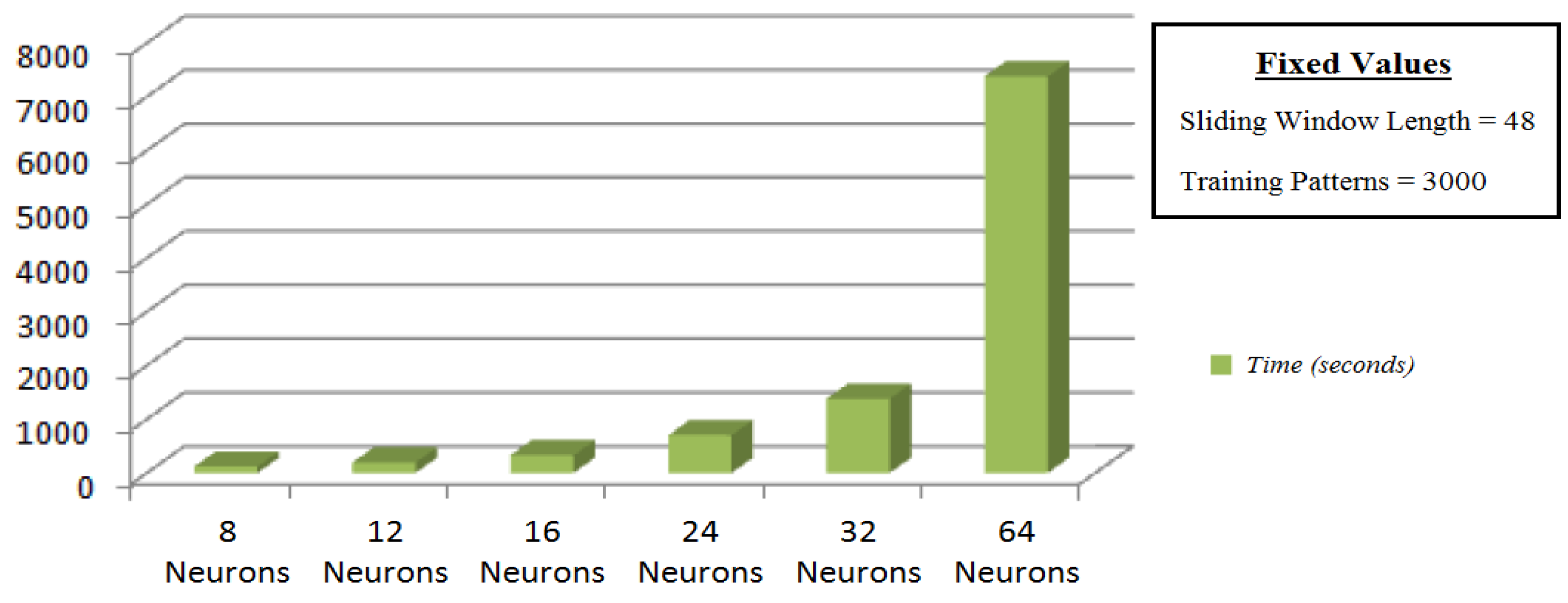
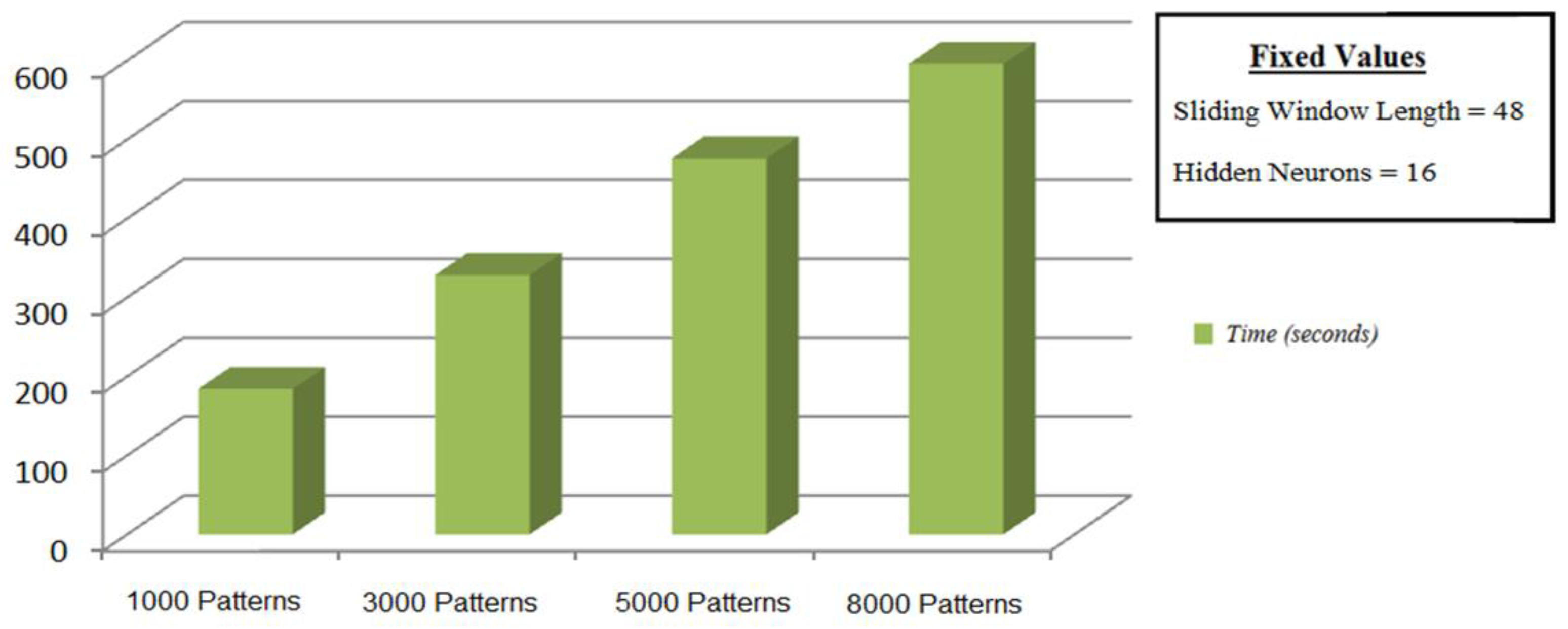
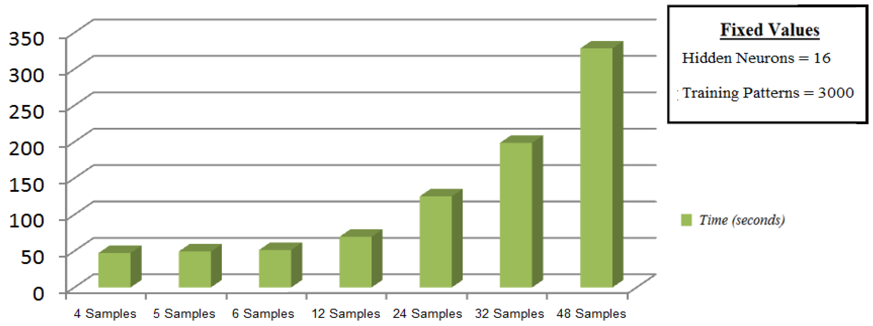
The study of training time is an important issue, being the latency between predictions, in particular, for short time predictions, a key aspect to reach a more accurate system. Moreover, it is necessary to add the test times, but it is insignificant compared to the training time. After the experiments, a key point is the number of hidden neurons, which is presented as the most influential parameter in the computational costs. This is because a linear increment in this parameter generates an exponential time increase in the phase of training as seen in Figure 11, Figure 12 and Figure 13. However, this increase of the parameters hardly affects the estimation phase, where the prediction time is almost immediate and answers are obtained in order of 0.04 s for the non-feedback modes. This is due to the execution in parallel which characterizes this type of architecture. Therefore, the latency in the estimation phase depends on the time in which the meteorological station provides new stimuli to the system being 30 min in this work.

The optimization using Adding-Score approach offers, as demonstrated above, improvements which are not too significant for the non-feedback modes. In addition, for the feedback modes, the use of this optimization contributes to minimize the errors introduced into the system through the use of estimated values as input values.

The goals of the research were satisfied due to the obtained results with an error below 0.30 °C (p-value = 0.15) for all cases of non-feedback modes versus the state-of-the-art which reach an error around 1 °C. For feedback modes, the results were lower than 1.5 °C for the first 48 samples, corresponding to 24 h prediction time. Likewise, the inclusion of combined input-stimulus improves the prediction accuracy and it is also presented as a rectifier method against input-patterns which present irregular behaviors. Additionally, a rigorous study of the behavior of feedback architectures into the field of prediction was carried out. The study achieves favorable results for the use of time continuous estimations. Additionally, the adaptation of a score-fusion method to these architectures has even offered better performance than the one obtained by the initial system, stabilizing the response of the feedback-methods. The standardization of input-data is recommendable as a procedure to reach systems with a faster and more stable convergence.

In

Table 14. Computational times for each mode.

Type of Mode	Training Time	Testing Time Per Sample (for 1000 Samples)
MODE.1	35.33 s	3.96 x 10−2 s
MODE.2	52.94 s	4.04 x 10−2 s
MODE.3	397.92 s	33.74 s
MODE.4	363.19 s	21.76 s

all computation times using MATLAB (Mathworks: Natick, MA, USA) in an ACER 3820TG (Intel Core i3 330M 2.13 GHz, 4 GB Ram, 500 GB HDD) can be observed:

It is observed as Modes without feedback are faster than Modes with feedback with the independence of the prediction for a short or large time. The difference is up to 10 times faster for training phase and 100 times for testing phase. From an absolute value point of view, the training times are shorter and the testing time can be considered as in real time. The accuracy for predicting on short time has a difference of 0.1 °C between Mode.1 and Mode.2, therefore, the feedback of Mode.2 gives a better accuracy, but a little high computational time than Mode.1 and the use of the optimal accuracy can be justified for this proposal.

As shown in

Table 15. Comparative with previous researches using ANN.

Reference	Error of Prediction
[6]	1 °C
[7]	2 °C
[11]	1 °C
[13] (same meteorological stations, without Score Fusion on ANN)	0.28 °C
[16]	0.01 °C
Our research (with Score Fusion on ANN)	0.13 °C

, our research, using Score Fusion on ANN, improves the results obtained by previous researches using ANN except for one. In addition, compared to dataset obtained from the same meteorological stations, Score Fusion reduce error obtained by 50%, demonstrating the goodness of the method. Respect to other researches, Score Fusion on ANN reduces the error to magnitudes of tenths.

5. Conclusions

This paper establishes two different acting lines. The first one is based on non-feedback modes, which are able to reach significant accurate temperature predictions throughout the day. For these modes, it is recommended to use small window size (4–6 samples), a number of hidden neurons between 8 and 12 and a dataset of patterns not less than 3000–5000 observations. In addition, it was demonstrated that the use of other influential elements improves the prediction.

The second one is based on feedback modes, which are useful for temperature forecasts in short-term. These modes can be employed in social area, being interesting in urban and agriculture areas, touristic sector or even serving as useful tool for emergency services to announce weather alerts. For these latter modes, it is recommended to use medium-sized windows (24–48 samples), a number of hidden neurons between 8 and 12 and also a dataset of patterns not less than 3000–5000 observations. In addition, for a combined input-stimulus, the sampling time parameter is only recommended.

This research using ANN with Score Fusion represents an improvement versus previous research using the same meteorological stations and ANN without Score Fusion.

As a future line of this research, it could be applied in energy efficiency. Serving as a supporting instrument to manage electrical power station, to improve the energy efficiency and to prevent peaks of electrical demand, assuring the sustainability of urban development.