Scale-Free Relationships between Social and Landscape Factors in Urban Systems

Abstract

Urban planners and ecologists have long debated the relationship between the structure of urban landscapes and social activities. There have, however, been very few discussions as to whether any such relationships might depend on the scales of observation. This work applies a hierarchical zoning technique to data from the city of Quito, Ecuador, to examine how relationships between typical spatial landscape metrics and social indicators depend on zoning scales. Our results showed that the estimates of both landscape heterogeneity features and social indicators significantly depend on the zoning scale. The mean values of the typical landscape metrics and the social indicators all exhibited predictable responses to a changing zoning scale, suggesting a consistent and significant scaling relationship within the multiple zoning scales. Yet relationships between these pairs of variables remain notably invariant to scale. This quantitative demonstration of the scale-free nature of the relationship between landscape characteristics and social indicators furthers our understanding of the relationships between landscape structures and social aspects of urban spaces, including deprivation and public service accessibility. The relationships between social indicators and one typical landscape aggregation metric (represented as the percentage of like adjacencies) were nevertheless significantly dependent on scale, suggesting the importance of zoning scale decisions for analyzing the relationships between the social indicators and the landscape characteristics related with landscape adjacency. Aside from this typical landscape aggregation metric, the general invariance to the zoning scale of relationships between landscape structures and socioeconomic indicators in Quito suggests the importance of applying these scale-free relationships in understanding complex socio-ecological systems in other cities, which are shaped by the conflated influences of both anthropogenic and natural factors. Moreover, this scale-free behavior of landscape–social relationships challenges the traditional modifiable area unit problem, and provides mechanistic insight into the conflicts and compatibilities between human activities and human-induced land use change.

1. Introduction

Spatial urban landscape metrics provide quantitative insights into complex natural systems, and are often used to characterize the heterogeneity of urban landscape composition and associated ecological processes [1,2,3,4,5,6]. Landscape ecologists and urban planners have long debated potential relationships between spatial patterns of urban development and ecological conditions, including the validity of spatial landscape metrics for purposes such as monitoring urban land use and sustainable urban planning [7,8,9]. Spatial landscape metrics can not only quantify ecological processes reflecting urban environmental change, but are also able to provide evidence of potential mechanisms linking urban form to social function. Furthermore, they can offer valuable insights into the resource distribution of urban socio-ecological systems by determining the distributional characteristics of energy, materials, or other properties [10,11,12]. Configurational characteristics may also influence demographic processes such as population growth, household locations, and migration [13]. Different landscape structures may lead to differences in economic development as a result of household income disparities [14]. The size of a single district within a city may influence gentrification processes of surrounding neighborhoods and result in the development of hierarchical structures that both promote and reflect differences in levels of accessibility to public services such as education or health [14,15]. Many previous studies that have examined the relationships between landscape configuration and social aspects such as urban poverty, health, or socioeconomic vulnerability [16,17,18,19] have done so on a qualitative level, yet often without quantitatively discussing how urban spatial metrics (such as composition or configuration) might characterize and influence social indicators. A truly integrative approach to identifying urban environmental heterogeneity demands that we address the quantitative relationships between urban spatial metrics and social activities, in order to provide concrete and meaningful knowledge for geographically contextualized urban planning, design, and management [20,21,22].

Spatial landscape metrics are useful for quantitatively describing and representing the heterogeneity of urban spaces. However, heterogeneity is also a function of scale [23,24,25,26], and the use of districts or blocks of fixed sizes is problematic for quantifying spatial landscape metrics. Several studies have clearly demonstrated that spatial metrics of community organization or landscape complexity differ with scale and scope [1,27,28]. This dependence of landscape heterogeneity on the scale of the zones used for its quantification reflects the well-known modifiable areal unit problem (MAUP) [29,30,31]. New technologies for user-controlled and flexible zoning schemes offer a practical solution to the MAUP. Automated zoning procedures, in particular, have been proposed to offer efficient, systematic, and objective methodologies for identifying functional zones based on social indicators such as population size, deprivation, or health [32,33,34]. Nevertheless, such zoning procedures still ignore more general issues of the representability of spatial landscape heterogeneity characteristics, especially in regard to whether or not a given set of boundaries makes any sense in relation to the spatial landscape metrics and processes relevant to the social activities that they represent.

One of the most powerful ways to understand the influence of landscape structures on socio-political processes is through cross-scale comparisons, as has been demonstrated by the relationships between spatial landscape metrics and socioeconomic indicators such as health outcomes, urban accessibility, and other social processes used to support social planning [35,36]. The present study therefore implements a hierarchical zoning strategy to analyze how quantitative relationships between spatial landscape metrics and social activities change across scales.

2. Study Area and Data Collection

Urban sprawl occurs around the world, and Latin America in particular is characterized by rapid urban growth and high inequality in terms of public services accessibility and other socioeconomic variables [37]. The capital city of Ecuador, Quito, is a representative example of how Latin American cities have faced significant growth in the last decades. The city has extended approximately 35 km in length and its suburban areas now occupy lands that only a few years ago were rural and agricultural areas. According to the Ecuadorian Institute of Statistics and Census, more than 1.5 million inhabitants live in Quito and its surrounding urban areas (Figure 1). However, considering the whole metropolitan district, including rural areas, the population is over 2 million. Some illegal constructions have gradually emerged in the peripheral areas of the city, mainly on the hills and steep lands. This dynamic landscape structure has generated obvious urban segregation in terms of social deprivation and public service inequality. It is thus worth investigating how the landscape structure characteristics differ in their corresponding social indicators connected to the urban environment.

Following a rights-based perspective of quality of life [38,39], good access to urban services is indispensable to ensure good conditions/prerequisites for quality of life. Keeping this in mind, we did a thorough and succinct literature review [39,40,41,42,43,44,45,46,47] and selected three indicators (deprivation, accessibility to healthcare services, and accessibility to educational services) to characterize the socioeconomic situation in Quito. These indicators support the identification of social inequalities and segregation with important implications for the sustainability and quality of life of a city [38,43,47]. We used data from 5000 census blocks, extracted from the 2010 Ecuadorian Population and Housing Census, as well as information regarding the locations of health and educational services, provided by the Ecuadorian Ministry of Health and the Ecuadorian Ministry of Education, respectively. Since all these indicators are elementary indicators based on census blocks (dissemination areas), our methodology is also transferable and may be applied to other Latin American cities. In addition, land survey data and 2010 Rapid Eye satellite data for Quito were provided by the Ecuadorian Ministry of Environment, and were used to extract information on land use and land cover (LULC). Spatial landscape metrics were estimated based on this LULC information.

3. Methods

We implement a hierarchical framework (shown in Figure 2) based on the combination of land use and land cover data with census data to explore how the zoning scale might influence the relationships between landscape heterogeneity features and the chosen social indicators. Four metrics of landscape configuration (including Shannon’s Diversity metric, Number of Disjunct Core Areas metric, Proportion of Like Adjacencies metric, Fractal Dimension metric) are described first, followed by methods for analyzing and aggregating three social factors (including deprivation, healthcare accessibility, and education accessibility). Finally, this research describes how social and landscape measures were combined within the automated zoning analysis and how the relationships between the spatial landscape metrics and social factors vary between different zoning scales. Integrating the concept of multiple zoning scales into the urban landscape–social relationships analysis is central to this framework, and it is important to investigate the multi-scale neighborhood effects on the complex urban system.

3.1. Analysis of Landscape Spatial Metrics

Categories of land use and land cover for Quito included residential areas, multi-type residential areas, industrial areas, cultivated areas, water areas, and vegetated areas including grass, eucalyptus, shrubbery, mountain shrubs, soil, and other vegetation cover.

The configurational properties of these different LULC classes were quantified using free Fragstats software (University of Massachusetts Amherst, Amherst, MA, USA) [48]. Fragstats quantifies landscapes in terms of both configuration and composition, with configuration further quantified in terms of the shape, area, and aggregation properties. For each of these four categories, we selected the single metric that most strongly correlated with all other metrics within that category. For the composition this was the Shannon’s diversity index (SHDI); for the shape this was the area-weighted mean patch fractal dimension index (FRAC_AM); for the core area it was the number of disjunct core areas (NDCA), and for aggregation it was the proportion of like adjacencies (PLADJ). Shannon’s diversity metric (SHDI; correlation with other aggregation metrics ≥0.8) reflects the landscape composition rather than the spatial configuration, and quantifies the amount of ‘information’ per individual landscape patch. The fractal dimension index (FRAC_AM; correlation with other shape metrics ≥0.355) equals the sum of the corresponding patch fractal dimension values multiplied by the proportional abundance of the patch. The number of disjunct core areas (NDCA; correlation with other core area metrics ≥0.32) quantifies how many small patches within a given interior belong to a large patch. The proportion of like adjacencies (PLADJ; correlation with other aggregation metrics ≥0.505) computes the sum of the diagonal elements of the adjacency matrix divided by the total number of adjacencies in such a way that landscapes containing greater local aggregations of patch types (for example, by having larger patches with compact shapes) will contain a higher proportion of like adjacencies than landscapes containing disaggregated patch types.

3.2. Social Indicators Estimation

We used census data and the location of healthcare and educational services to estimate three social indicators that are reflective of more general yet intangible societal processes: a composite indicator of deprivation (DP); and indicators of accessibility to healthcare services (DH) and educational services (DE).

The composite indicator of deprivation was measured by combing four simple indicators: (1) the percentage of houses without access to the sewerage system; (2) the percentage of houses without a connection to the electrical system; (3) the percentage of houses without a connection to the drinking water supply system, and (4) the percentage of houses without a garbage collection service. These indicators were chosen because they are related to basic human needs, represent social disadvantages, and can be related to health issues [38,39,47,49,50,51]. Information pertaining to these indicators was extracted from the 2010 Ecuadorian Population and Housing Census.

The deprivation information was geocoded in census tracts and compiled in the shapefile of the study areas. The variance inflation factors (VIFs) for all indicators confirmed no strong co-linearities between the selected indicators, enabling them all to be used in the composite indicator of deprivation, constructed by adding the four indicators and normalizing the result to the unit scale. The final composite indicator of deprivation then has values between 0 and 1, where values closer to 1 represented higher levels of social deprivation.

The accessibility indicators (to both health and educational services) were calculated in terms of Euclidean distances between the centroids of each census block and the location points representing the nearest healthcare or educational services.

3.3. AZPTool—Automatic Zoning Software

The automatic zoning procedure (AZP) (University of Southampton, UK) was developed by Openshaw [31] to explore scale and aggregation effects on the choice of zonal boundaries. This was extended by Martin [33], who developed an automated zone matching (AZM) algorithm that iteratively combines target population sizes, zonal compactness and other variables into the zone design process. This study used the AZTool system, based on the AZM algorithm, which has the advantage of minimizing the mismatch between different zones [33,52]. We created zones that maximized the internal homogeneity of independent variables. This regionalization algorithm is a heuristic procedure involving the following steps [30,31,32,33]:

• Step 1. Select zone design options and targets.

  ○

  (i) Set the threshold variable which can indicate the homogeneity of the boundary;

  ○

  (ii) Set the minimum and maximum threshold of target value M to randomly generate M small zones from the original zoning system N (M < N);

  ○

  (iii) Set the iteration number to control the regionalization process.

• Step 2. List the M regions.
• Step 3. Randomly select and remove any region from this list.
• Step 4. Identify zones that border members of region K that could be moved into region K while maintaining the internal contiguity of the donor region(s).
• Step 5. Select zones randomly until one of the following conditions is met: (1) there is a local improvement in the current value of the objective function (seen Formula (1) and (2)); (2) a move that is at least as good as the current best. Then repeat step 5 until the list ends.
• Step 6. When the list for region K is exhausted return to step 3, select another region, and repeat steps 4–6.
• Step 7. Repeat steps 2–6 until no further improvement can be made or a maximum number of iterations is reached.

The AZTool maximizes the internal homogeneity of zones as quantified by the parameter-intra-area correlation (IAC). The IAC depends on the variable ${\partial }_k$, which is the contribution of category k to the IAC (shown in Equation (1)):

$${\partial }_k=\frac{\frac{1}{M-1}{\displaystyle \sum _{g=1}^M{N}_g{(P_{gk}-P_k)}^2}}{(\overline{N}*-1)P_k(1-P_k)}-\frac{1}{(\overline{N}*-1)},$$

(1)

where M is the number of areal units in the original zoning system, $N_g$ is the value of the target threshold variable in the areal unit g, $\overline{N}*$ is the mean of target threshold variable in the original zoning system, $P_{gk}$ is the value of homogeneity feature k in the areal unit g, and $P_k$ is the overall mean of the homogeneity feature k. This formula is approximately the ratio of the area-level variance to the individual-level variance. Having calculated the intra-area correlations ${\partial }_k$ for each zoning variable, an overall intra-area correlation measure $\partial$ can be calculated as in Equation (2), which then provides a statistically valid measure with which to compare different zoning scales with different target features:

$$\partial =\frac{1}{k-1}{\displaystyle \sum _{k=1}^K(1-P_k)}{\partial }_k$$

(2)

Each potential modification to the zonal configuration is evaluated in terms of its marginal impact on ICA, and AZM provides various constraints and values for the control of zone design. In our study, the four spatial landscape metrics (FRAC_AM, NDCA, PLADJ, and SHDI) and the three social indicators (DP, DE, and DH) were chosen as the threshold variables to construct separate zoning schemes.

The choice of these design constraints and target values is subjective, but serves to ensure consistency between different zone design runs. Values were selected to achieve reasonably compact and hierarchical levels, in order to quantify the effect of the MAUP on resultant relationships in a consistent and reproducible way. Accordingly, the 5000 original census blocks were aggregated into six hierarchical levels containing 130, 420, 800, 1000, 2000, and 3500 zones.

3.4. Statistical Tests

We first tested the scale-dependence of the four landscape metrics and the three social indicators, hereafter referred to as landscape/social (LS) variables, by applying linear regressions to the logarithm of the zoning scale (quantified as the number of polygons listed above). The data for each scale were grouped into 130 evenly-spaced bins (equal to the number of points at the coarsest zoning level), so that regressions considered equal numbers of data points for each zoning level.

We then considered the mutual influences of other LS variables and zoning scales by performing multiple linear regressions (MLRs) between each pair of variables and including the zoning scale as an additional independent variable. For the n = 7 variables, this involved n(n − 1)/2 = 21 MLRs, each of which had one landscape metric or social indicator as the dependent variable and two independent variables, namely the zoning scale and the other LS variable. The relative influences of the zoning scale and the other LS variables were then quantified by comparing T-statistics. The MLRs also considered potential interactions between scale and the other independent variables, with relative effects of interactions also quantified by associated T-statistics.

Finally, we examined whether the scale directly affects relationships between the different LS variables by calculating linear regressions of each pair of LS variables for each distinct zoning scale. As described in the first paragraph above, all variables had equal numbers of observations for each scale, enabling T-statistics from the linear regressions to be directly compared across scales. The T-statistics quantify the strength of the relationship between each pair of LS variables at each zoning scale. Linear regressions were subsequently performed through each series of T-statistics to ultimately quantify the extent to which relationships between each pair of variables were themselves dependent on the zoning scale. Relationships between LS variables for any given scale may not be significant, in which case the T-statistics may not be presumed meaningful. These subsequent regressions therefore considered only those T-statistics representing significant relationships at p = 0.05.

4. Results

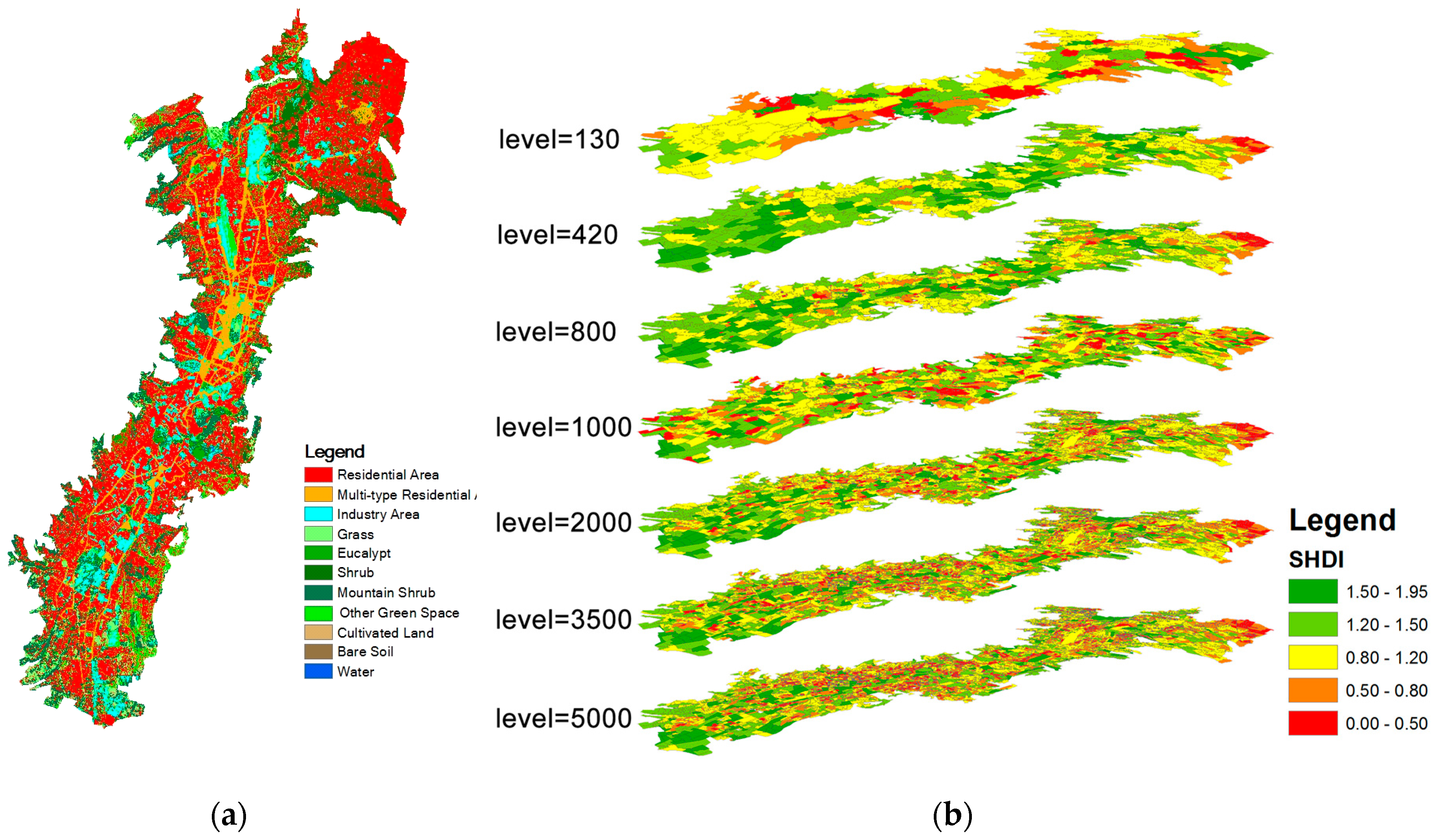
4.1. The Influences of the Zoning Effect on Landscape Metrics Estimation

As shown in Figure 3a, the top three land use and land cover (LULC) types in Quito were residential areas, other green spaces, and mountain shrub areas, making up 46.38%, 12.53%, and 11.28%, respectively; industrial areas (8.38%), shrub areas (7.1%), multiple-use residential areas (6.64%), grassland (5.04%), eucalyptus (1.82%), cultivated land (0.66%), and bare soil (0.15%) are the other LULC types, followed by water, which makes up the smallest percentage of the LULC with only 0.02%. Residential areas are distributed all over the city of Quito, but are particularly concentrated in the northern area and the suburban area of the city. Industrial and commercial areas, as well as low-income residential areas are mainly concentrated in the southern part of Quito. Figure 3b provides an example of SHDI representations at seven zoning levels (130, 420, 800, 1000, 2000, 3500, and 5000) produced through the aggregation process in the original census blocks. The spatial pattern results of the SHDI in these five zoning scales, which range from 0 to 1.92, lead to very different spatial cluster distributions.

4.2. Scale-Dependence of Landscape and Social Factors

All four landscape metrics and all three social indicators were significantly dependent on the zoning scale (Figure 4 and Figure 5, respectively). All relationships with the landscape metrics were highly significant (p < 10⁻¹⁰). The notably low values of all strengths of relationship (given in the legend of Figure 4 and Figure 5) reflect the fact that these spatial metrics vary to a far greater extent across the study area than they do across zoning scales; that is, spatial heterogeneity within each zone is far greater than systematic variation between zones. The high significance of all observed relationships nevertheless shows that the zonal scale does significantly influence all landscape and social indicators.

Finer zoning scales (that is, those containing a greater numbers of polygons) were associated with increases in both fractal dimension (FRAC_AM) and number of disjunct core areas (NDCA), yet with decreases in both landscape diversity (SHDI) and the proportion of like adjacencies (PLADJ). In contrast, all three social indicators (DE, DH, and DN) significantly decreased at finer zoning scales.

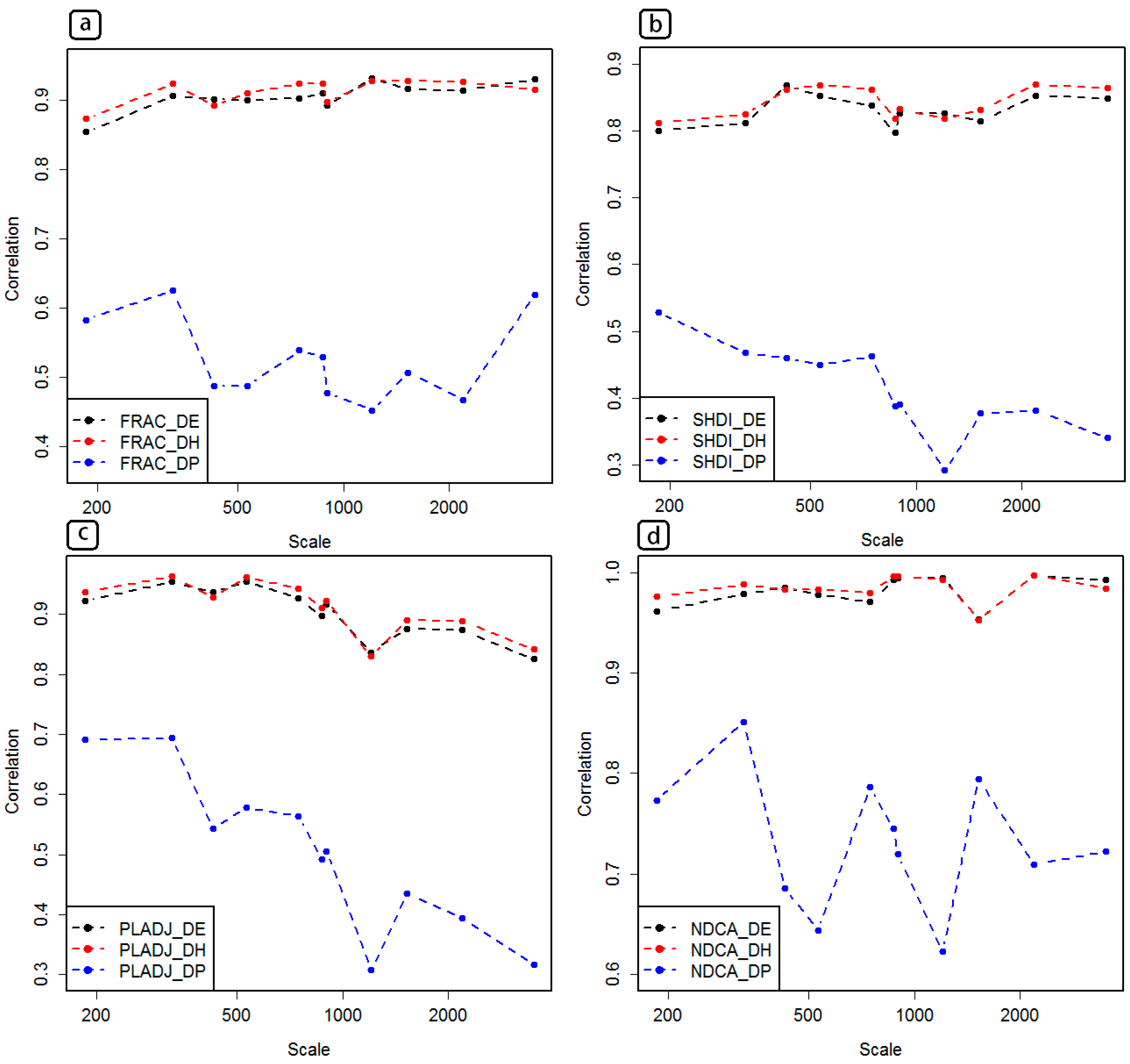
4.3. The Mutual Influences of LS Variables and the Zoning Scale

Multiple linear regressions (MLRs) for each landscape/social (LS) variable using both zoning scale and every other LS variable in combination yielded T-statistics indicating that the mutual influences of the LS variables on one another was always stronger than the influence of the zoning scale (

Table 1. T-statistics for the mutual influence of variables and the zoning scale.

Independent Variable	Dependent Variable	T (Variable)	T (Scale)	T (Variable & Scale)
FRAC_AM	SHDI	34	−14	−13
FRAC_AM	NDCA	9	−6	7
FRAC_AM	PLADJ	31	−9	−8
FRAC_AM	DE	41	19	−27
FRAC_AM	DH	41	16	−26
FRAC_AM	DP	19	9	−14
SHDI	NDCA	5	10	7
SHDI	PLADJ	23	13	4
SHDI	DE	22	20	−11
SHDI	DH	23	20	−11
SHDI	DP	17	13	−12
NDCA	PLADJ	24	−12	−10
NDCA	DE	55	13	−37
NDCA	DH	57	10	−38
NDCA	DP	27	6	−20
PLADJ	DE	35	21	−21
PLADJ	DH	36	22	−21
PLADJ	DN	22	17	−18
DE	DH	61	−15	6
DE	DN	22	5	−13
DH	DP	23	7	−14

), with the single exception of SHDI being more strongly influenced by scale than by NDCA. (The T-statistics of Table 1 reflect relationships that were all entirely significant, with the largest p-value < 10⁻⁵). Taken together, T-statistics for the mutual influence of other variables were significantly higher for the influences of other variables (mean T = 29.9) than for the influence of the scale (mean T = 13.2; T-test for differences: df = 25, T = −4.9, p < 10⁻⁴). In the context of these pair-wise comparisons, scale thus explained less of the variance in the LS variables than did the influence of other LS variables.

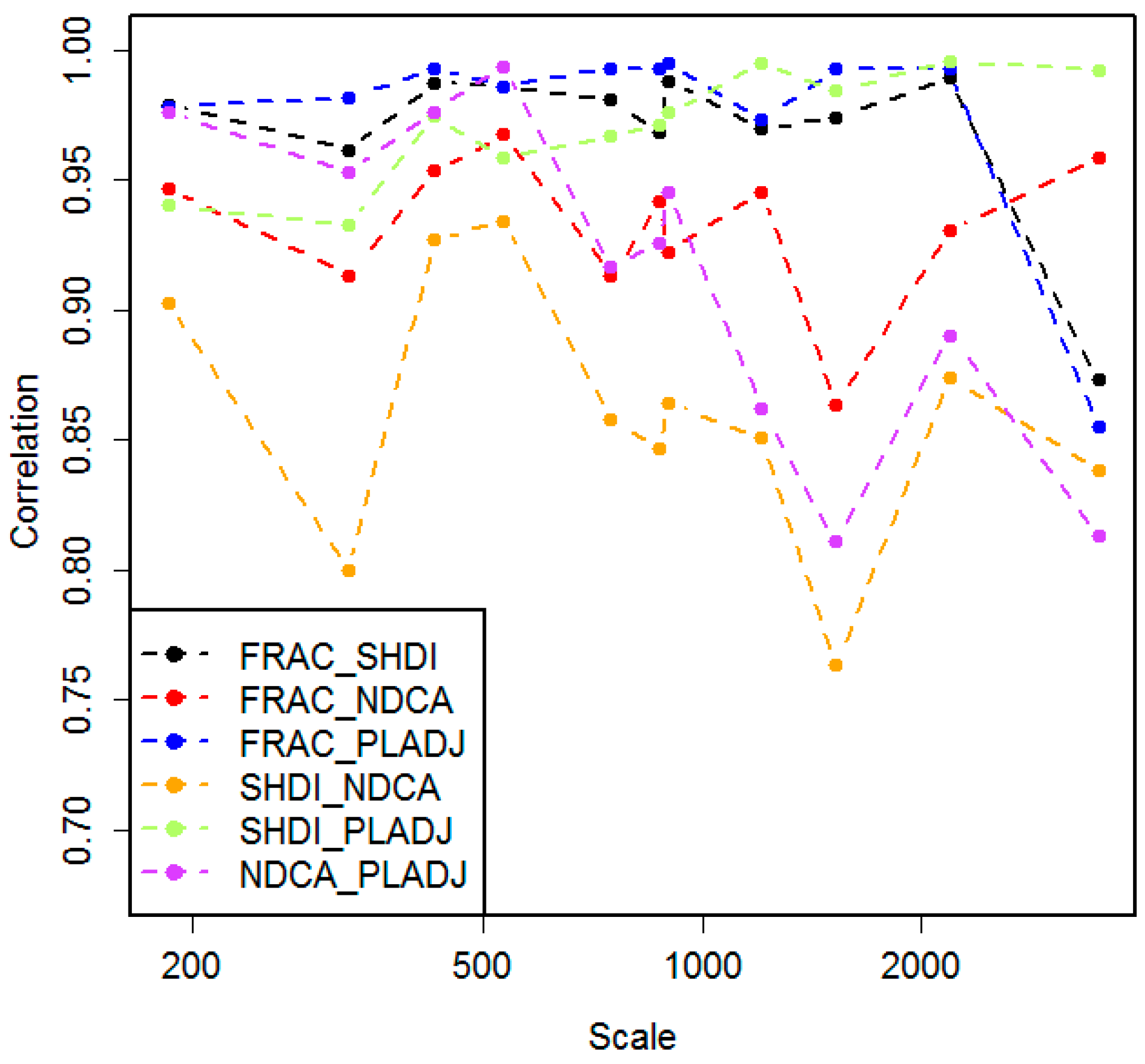
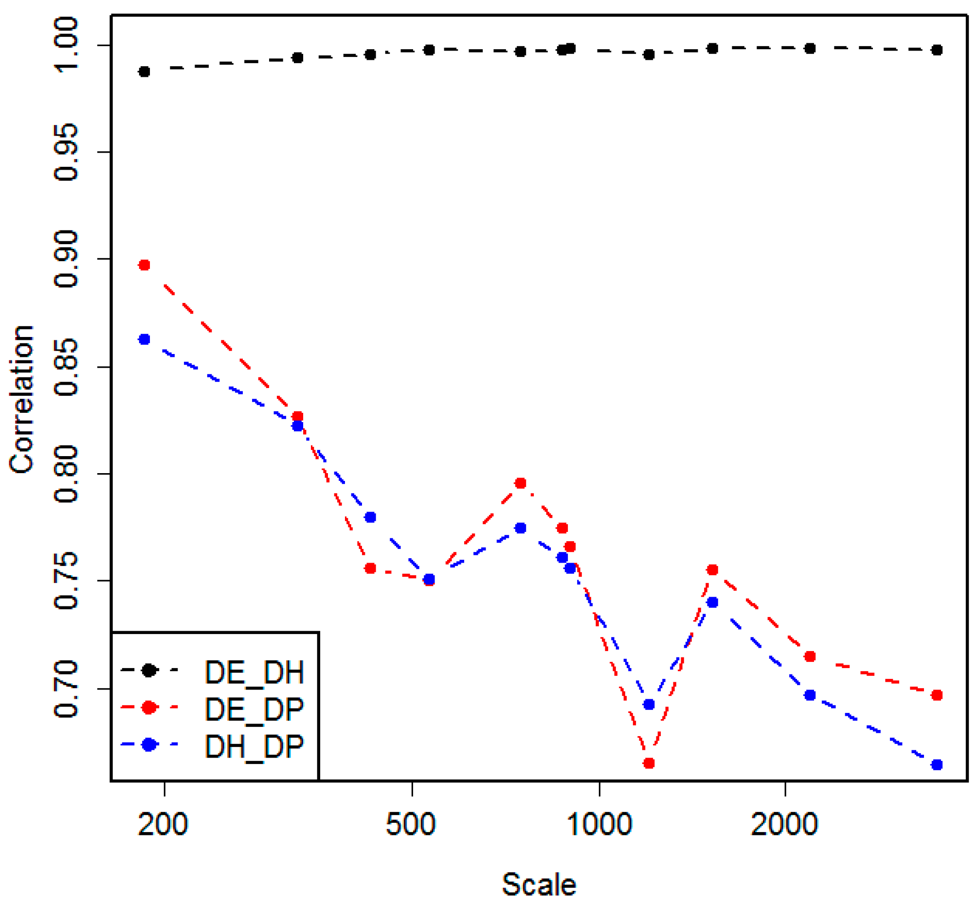
4.4. The Scale-Dependence of Relationships between LS Variables

Finally, linear regressions were calculated between all LS variables for each zoning scale and strengths of relationship were quantified in terms of T-statistics. These T-statistics were able to be directly compared across scales because sample sizes were identical in all cases (equal to 130 points). The scale-dependence of the relationships between the landscape metrics is shown in Figure 6; that of the relationships between the social indicators in Figure 7; and that of the relationship between landscape and social measures in Figure 8. (To aid visual interpretation, the strengths of relationship in all of these figures are depicted in terms of correlation coefficients, while all statistics were calculated from associated T-statistics.)

The relationships between the different landscape variables generally remained independent of the zoning scale (Figure 6), with the exception of SHDI-PLADJ (R² = 0.61, p = 0.005). Relationships between all other landscape metrics attained maximal correlations with a scale of R² < 0.25 (p > 0.06). By contrast, relationships between social indicators were more strongly influenced by scale, and, in fact, had average T-statistics for dependence on scale of T = 4.8 in comparison with equivalent values for landscape variables of T = 1.4 (T-test for differences in these statistics: T = 2.8, df = 3.1, p = 0.06). The weakest dependence on scale of a relationship between social indicators corresponded to a correlation of R² = 0.58 (p = 0.006). Relationships between social indicators were thus significantly dependent on the zoning scale in all cases.

Finally, seven of the 12 relationships between landscape and social indicators were not significant, while five were. Of these latter five, however, three described the relationships with PLADJ. Excluding this variable, only two of the remaining 9 variable relationships indicate a significant dependence on scale (FRAC_AM-DE and SHDI-DP). This supports the general conclusion that relationships between landscape metrics and social indicators generally remained independent of the zoning scale. Reasons for the significant dependence on PLADJ are discussed below.

5. Discussion

5.1. Scale-Dependent Landscape Metrics

The effect that changing the scale has on landscape metrics has generally been considered in terms of both grain size and extent, yet rarely in terms of the zoning scale. Our study thus examined how a typical group of landscape metrics responds to the zoning scale [53]. All landscape metrics exhibited significant relationships with the zoning scale, with mean values of metrics of both contagion (PLADJ) and diversity (SHDI) increasing with increasing zoning scale (that is, increasing with a decreases in the numbers of zoning units), and mean values of shape and core area metrics (FRAC_AM and NDCA, respectively) decreasing with increasing zoning scale. Similar results for metrics of diversity, shape, and core area have been reported by Wu et al. [23] and Alhamad et al. [54].

Notably, although Wu et al. [23] pointed out the erratic and generally unpredictable behavior of contagion metrics in response to changing grain size, it was possible within the present study to derive explicit scaling functions for the contagion metric used here across multiple zoning scales in Quito. This may suggest that different aggregation methods have significant effects on the characteristics of landscape metrics in response to changes in scale.

5.2. Scale-Dependent Social Indicators

Previous research on the spatial concentration of social and economic conditions has resulted in several important questions regarding the role of spatial scale. Our results show that the means values of all three social indicators quantified here (deprivation and accessibility to both healthcare and educational services) significantly increased with increasing zoning size. These social indicators thus manifest a general and predictable tendency across multiple scales of ‘neighborhood’ units, confirming a previous assertion that cross-scale interaction studies provide useful insights into complex urban systems [55,56].

5.3. Scale-Free Relationships between Social and Landscape Factors in Urban Systems

Although the significant scale-dependence of landscape metrics and social indicators supports the claim that there is no single ‘correct’ or ‘optimal’ scale for characterizing and monitoring complex urban systems, the scale-free relationships between landscape metrics and social indicators discerned here are likely to be of immediate interest to landscape ecologists aiming to understand relationships between demographic changes and transformations of landscape heterogeneity.

The effects of the relationships between landscape metrics and social indicators on the zoning scale can be grouped into three general types: type I, for which all relationships are scale-free; type II, for which some but not all relationships are scale-free; and type III, for which all relationships manifest significant dependence on scale.

The first type (type I) included all relationships with the NDCA metric (number of disjunct core areas), with which all correlations with social indicators (including the composite indicator of deprivation and the accessibility indicators) were very strong while remaining statistically independent of the zoning scale. This confirms that the NDCA metric indeed provides a highly useful metric of habitat quality [57], because its relationship with social processes is independent of the scale of observation. NDCA is simply the total number of disjunct core areas contained within a single zone. Low values of NDCA in Quito arose in regions of low deprivation and high accessibility to health and educational services, mainly in residential areas. In contrast, high values of NDCA were associated with high deprivation and low accessibility to health and educational services in urban areas with a high vegetation cover. The scale-free relationships between NDCA and social indicators actually provides a first insight into likely relationships between the spatial structure and social characteristics of neighborhoods that may lead to an understanding of how social, health, and ecological processes might influence the quality of life in Quito.

The second type (type II) of relationships included the relationships between social indicators (including the composite indicator of deprivation and accessibility to education services) with the fractal dimension index (FRAC_AM), which shows scale-free relationships with deprivation (DP) and accessibility to healthcare services (DH). However, the relationships between the FRAC_AM with accessibility to education services (DE) increased significantly with increasing zoning scale. The areal-weighted mean patch fractal dimension (FRAC_AM) metric provides a way to summarize the shape complexity of patches in a landscape [58]. As built-up areas are more intensively and regularly aggregated than the natural resources across all zoning scales, the areal-weighted mean FRAC_AM metric in the residential areas in Quito is generally lower than in the vegetated areas. FRAC_AM metric significantly decreased with increases in zonal sizes, reflecting the agglomeration of built-up areas into large, more densely built-up patches. The high-degree of correlation and scale-free relationship between FRAC_AM and the composite deprivation indicator further confirm the dominance of residential areas in Quito, with high density built-up areas closely related to low deprivation states. The significant dependence on the zoning scale of the relationships between FRAC_AM and accessibility to health and educational services likely reflects the highly uneven distributions of health and education services within the study area.

Relationships between socioeconomic indicators and the Shannon diversity index (SHDI) were also only partly independent of the zoning scale. While most of the relationships were generally independent of scale, the relationship between SHDI and the composite indicator of deprivation depended significantly on the zoning scale. The SHDI index accounts for both the abundance and evenness of land cover types. In the original census blocks, the diversity in residential areas with low levels of deprivation is much lower than the equivalent diversity in suburban areas with higher proportions of natural land cover. Increasing the zone size resulted in the SHDI metrics becoming increasingly influenced by different land use covers, such as multiple types of residential, industrial, or vegetated areas, which illustrates the observed scale-dependence of the relationship between SHDI and deprivation. Similar results in relation to land cover, as quantified by the SHDI metric, have been observed by Nagendra [59]. The scale-dependent relationship between SHDI and deprivation may also reflect the aspects of viability and the social–ecological resilience of landscape.

The third and final category (type III) of relationships represents those where all relationships between landscape and socioeconomic metrics were significantly dependent on scale, most notable for the proportion of like adjacencies (PLADJ). This metric has been widely used to quantitatively assess changes in landscape patterns associated with urbanization [58], mainly because it has the advantage of being intuitive and computationally simple. Low PLADJ values correspond to high fragmentation or areas otherwise comprising numerous distinct units [59], such as regions of scattered urban sprawl in suburban Quito. Nevertheless, although the PLADJ metric can describe whether inhabited areas are maximally contagious at each zoning scale, its measurement is sensitive to other types of large land use patches, such as industrial or park areas, which also obviously influence the degree of conjunction with the surrounding patches. The small patchiness of residential areas may show up as disaggregated in small zoning scales while being conjunction in larger zoning scales. In Quito, as the zoning size increases, residential areas gradually become the dominant land cover type that maximally joins with other land use classes in each zoning areas, leading to the relationships between PLADJ and social indicators becoming steadily stronger. The PLADJ is frequently used to categorize urbanization in terms of urban fragmentation, but the scale-dependent relationships revealed here show that associations between built-up areas and social processes are in this sense dynamic and dependent on scale.

The landscape of Quito thus reveals how relationships between landscape metrics and social indicators are shaped by both anthropogenic and natural factors, and, in particular, by interactions between these two. The relationships between social indicator and spatial landscape metrics on the multiple zoning scales revealed here may be extrapolated to suggest the likely directionality or orientation of landscape patterns across multiple scales in other urban systems subject to analogous urbanization process to Quito.

5.4. Complex Urban Systems: The Issue of Zoning Scale

It is becoming increasingly clear that current knowledge and the perspective of a human-dominated system is insufficient, particularly regarding the scale mismatch problems behind the different roles of urban socio-ecological systems functions [60,61]. This paper has highlighted how important the scale is when studying social and landscape relationships and how important it is to consider scale issues in urban planning. The prevalence of cross-scale interaction studies means that the most useful insights into the complex urban system comes from multi-scale studies [53,54]. The hierarchical framework in this study has captured the scale-free behaviors concerning the connections and organization between natural entities (e.g., landscape configuration and composition) and anthropogenic derivatives alike (e.g., urban poverty, public education service and public healthcare service). Such scale-free relationships likely also suggest that landscape properties, functions and processes have been strongly influenced by human activities in similar ways across a wide range of scales. This new view of the city structures and dynamics can offer urban planners unexpected perspectives and aid in improving the quality of life in cities.

Neighborhood is most often referred to as the ‘place bases’ or the ‘contextual unit’ of urban segregation analyses. The neighborhood delineation is an essential prerequisite to the implementation of public health policy [62] and urban planning policy for the well-being of citizens [63,64]. Many previous neighborhood analyses only combined multi-dimensional socioeconomic indicators (e.g., income, access to clean water, electricity, education, health care), based on their spatial correlations and spatial heterogeneities [65,66,67,68], to delineate the socially meaningful neighborhoods. Whether the spatial landscape features of urban ecological environments can be confirmed to account for neighborhood-level variations is still in its theoretical infancy, we still lack well-developed ‘theories of the middle-range’ that can systematically delineate the spatial unit combining different social and landscape characteristics with other contextual characteristics [69,70]. Zoning-based organization systems in this study provide a new approach to understanding the hierarchical characteristic variability of neighborhoods. It is important to consider the whole study area, which was stratified into hierarchical ‘neighborhood’ units, in order to characterize the spatial landscape features with minimal socioeconomic development bias, and to avoid spurious relationships between variant attributes in aggregating different neighborhood units.

The findings of the three kinds of relationships between landscape metrics and social indicators can support several specific insights with implications for urban planning. For example, the type I scale-free relationships have important implications for answering some decision making questions, such as whether the same urban land uses with several core areas can be functional at several scales? Our results suggest that it is possible. As natural core land covers (e.g., forests) with compact shapes are more resilient to harms (e.g., fires), and this structural reliance could be assigned to several scales, compact urban structures may be resilient to specific damages at different scales. The type II relationships can function as an indicator for measuring the urbanization progress. When the fractal dimension of land use and land cover is generally inconsistent with the socioeconomic activities in other case studies in future, it may imply an urbanization process that leads to built-up areas being more intensely and regularly aggregated than the natural resources across all zoning scales. The type III relationships suggest that it is necessary to take the scale issue into consideration if applying some specific landscape metrics (e.g., PLADJ) when describing the landscape–social relationships. Especially urban areas with fragmented land use may represent different social dynamics across different scales. To deal with such situations, dividing the city into big administrative zones may be more manageable for decision makers.

An important aim for future studies should be to better understand what kinds of socio-ecological environments can be represented as scale-free fractal structures. Although interactions between social activities and landscape heterogeneity have been subject to extensive previous consideration [71,72], the dependence of their relationship at changing domain scales has rarely been reported on, either due to difficulties in terms of data or computation, or due to difficulties in identifying appropriate domains of scale [73]. In this study, integrating spatial landscape metrics and social indicators into an automatic zoning procedure represents a first attempt to link the contexts of the social and landscape characteristics into a multi-scale urban regionalization, which enables the quantitative exploration of the scaling relationships between complex socio-ecological urban processes.

Automatic zoning procedures can take into consideration potential relationships and homogeneity characteristics of inputs, and can allow zones to be aggregated in a hierarchical way. However, identifying suitable zoning scales for landscape-social analysis is still not easy, as parameters are required for automatic zoning procedures to remain subjective to some extent. Although the multi-scale zoning levels used herein were determined through several tests, the uncertainty and robustness of zonation aggregation remain important aspects for future research to address. Moreover, while the shapes of zoning may change drastically depending on the procedure of zoning aggregation, the specific landscape metrics associated with various landscapes may also change in different contexts.

Another issue to understand here is whether spatial patterns of social dynamics may also show fractals’ behaviors not only in pre-defined administrative areas (e.g., census block) but in other zoning scales too. Area-level social indicators are usually expressed in pre-defined administrative areas such as census blocks. It is expected that census blocks have more simple shapes, that is, lower values of fractal dimension. This research thus aggregated the hierarchical zoning levels based on the census block. Nevertheless, some scholars have questioned the ability of census blocks to capture basic functional socio-ecological units [74,75]. More and more relevant social, economic, political and ecological indicators in different study areas should be taken into consideration in the future to determine the causes of the socio-ecological factors in the context of the complex urban system, including questions such as: At which cross-scale scope may the urban landscape characteristics be used to determine the type of social network? Or in which range of zoning size does the landscape patches correspond well to the social public services organization? This new view of the city structures and dynamics can offer a solution to handle the sustainable regional partition problem between landscape biodiversity protection and public service construction, or between reducing the urban poverty and scientifically exploiting the natural resources.

6. Conclusions

We are living in an era where the main problems of sustainability can be resolved in cities. Major conversations of urban sustainability and planning for development are related to inequality and social resilience. Critical points in terms of urban studies are the need for multi-scale perspectives and the application of mixed methods. The methodology presented in this study addresses both these issues.

We applied an automatic zoning procedure to aggregate the census blocks into multiple zoning scales. T-statistics revealed that both landscape metrics and social indicators depend strongly on the zoning scale. Taken alone, this result suggests that any particular scale chosen for the measurement of spatial patterns may be inappropriate or difficult to apply in different environments. Although some aspects of landscape and social measures seem more generally predictable across zoning scales, the scaling behaviors of landscape metrics and social indicators will likely differ in different urban systems, suggesting the abiding importance of investigating the scaling behaviors of such metrics in different urban environments.

However, regardless of such potential scale-dependence of individual landscape or social indicators, relationships between the two classes of metrics within the present study generally remained independent of the zoning scale. This scale-free behavior challenges the modifiable unit area problem, enhances understanding of the causes and consequences of spatial heterogeneity and how they vary with scale, and has important implications for the management of both natural- and human-dominated environments. Through combining remote sensing data and statistical census data from Quito, the results of this study are expected to assist local officials in their understanding of urban dynamics, and, in so doing, to promote future sustainable growth.

The rapid development of earth observation technologies enables increasing amounts of spatio-temporal data to be used as a basis for modeling urban ecosystems. Relationships between landscape structures and characteristics of human societies will accordingly become increasingly easy to quantify more accurately, enhancing the mechanistic understanding or drivers and services of complex urban systems.

References

1. Wiens, J.A.; Milne, B.T. Scaling of ‘landscapes’ in landscape ecology, or, landscape ecology from a beetle’s perspective. Landsc. Ecol. 1989, 3, 87–96. [Google Scholar] [CrossRef]
2. Wiens, J.A. Spatial Scaling in Ecology. Funct. Ecol. 1989, 3, 385–397. [Google Scholar] [CrossRef]
3. Wagner, H.H.; Fortin, M.-J. Spatial Analysis of Landscapes: Concepts and Statistics. Ecology 2005, 86, 1975–1987. [Google Scholar] [CrossRef]
4. Blaschke, T. The role of the spatial dimension within the framework of sustainable landscapes and natural capital. Landsc. Urban Plan. 2006, 75, 198–226. [Google Scholar] [CrossRef]
5. Nuissl, H.; Haase, D.; Lanzendorf, M.; Wittmer, H. Environmental impact assessment of urban land use transitions—A context-sensitive approach. Land Use Policy 2009, 26, 414–424. [Google Scholar] [CrossRef]
6. Syrbe, R.-U.; Walz, U. Spatial indicators for the assessment of ecosystem services: Providing, benefiting and connecting areas and landscape metrics. Ecol. Indic. 2012, 21, 80–88. [Google Scholar] [CrossRef]
7. Lausch, A.; Herzog, F. Applicability of landscape metrics for the monitoring of landscape change: Issues of scale, resolution and interpretability. Ecol. Indic. 2002, 2, 3–15. [Google Scholar] [CrossRef]
8. Leitão, A.B.; Ahern, J. Applying landscape ecological concepts and metrics in sustainable landscape planning. Landsc. Urban Plan. 2002, 59, 65–93. [Google Scholar] [CrossRef]
9. Fragkias, M.; Seto, K.C. Modeling Urban Growth in Data-Sparse Environments: A New Approach. Environ. Plan. B Plan. Des. 2007, 34, 858–883. [Google Scholar] [CrossRef]
10. Vaz, A.S.; Marcos, B.; Gonçalves, J.; Monteiro, A.; Alves, P.; Civantos, E.; Lucas, R.; Mairota, P.; Garcia-Robles, J.; Alonso, J.; et al. Can we predict habitat quality from space? A multi-indicator assessment based on an automated knowledge-driven system. Int. J. Appl. Earth Obs. Geoinf. 2015, 37, 106–113. [Google Scholar] [CrossRef]
11. Vaz, E. The future of landscapes and habitats: The regional science contribution to the understanding of geographical space. Habitat Int. 2016, 51, 70–78. [Google Scholar] [CrossRef]
12. Cirella, G.T. Developing a Quantitative Multi-Criteria Method of Sustainability Assessment: With Application in Queensland, Australia; Griffith University: Logan, Australia, 2010. [Google Scholar]
13. Ktitorov, P.; Bairlein, F.; Dubinin, M. The importance of landscape context for songbirds on migration: Body mass gain is related to habitat cover. Landsc. Ecol. 2007, 23, 169–179. [Google Scholar] [CrossRef]
14. Iverson, L.R.; Cook, E.A. Urban forest cover of the Chicago region and its relation to household density and income. Urban Ecosyst. 2000, 4, 105–124. [Google Scholar] [CrossRef]
15. You, H. Quantifying urban fragmentation under economic transition in Shanghai city, China. Sustainability 2016, 8, 21. [Google Scholar] [CrossRef]
16. Cushman, S.A.; Landguth, E.L. Spurious correlations and inference in landscape genetics. Mol. Ecol. 2010, 19, 3592–3602. [Google Scholar] [CrossRef] [PubMed]
17. Lambin, E.F.; Meyfroidt, P. Land use transitions: Socio-ecological feedback versus socio-economic change. Land Use Policy 2010, 27, 108–118. [Google Scholar] [CrossRef]
18. Frumkin, H. Urban sprawl and public health. Public Health Rep. 2002, 117, 201–217. [Google Scholar] [CrossRef]
19. Hall, G.B.; Malcolm, N.W.; Piwowar, J.M. Integration of Remote Sensing and GIS to Detect Pockets of Urban Poverty: The Case of Rosario, Argentina. Trans. GIS 2001, 5, 235–253. [Google Scholar] [CrossRef]
20. Lugeri, F.R.; Farabollini, P.; Greco, R.; Amadio, V. The Geological Characterization of Landscape in Major TV Series: A Suggested Approach to Involve the Public in the Geological Heritage Promotion. Sustainability 2015, 7, 4100–4119. [Google Scholar] [CrossRef]
21. Loures, L.; Loures, A.; Nunes, J.; Panagopoulos, T. Landscape Valuation of Environmental Amenities throughout the Application of Direct and Indirect Methods. Sustainability 2015, 7, 794–810. [Google Scholar] [CrossRef]
22. Hacker, K.P.; Seto, K.C.; Costa, F.; Corburn, J.; Reis, M.G.; Ko, A.I.; Diuk-Wasser, M.A. Urban slum structure: Integrating socioeconomic and land cover data to model slum evolution in Salvador, Brazil. Int. J. Health Geogr. 2013, 12, 45. [Google Scholar] [CrossRef] [PubMed]
23. Wu, J.; Shen, W.; Sun, W.; Tueller, P.T. Empirical patterns of the effects of changing scale on landscape metrics. Landsc. Ecol. 2002, 17, 761–782. [Google Scholar] [CrossRef]
24. Herold, M.; Couclelis, H.; Clarke, K.C. The role of spatial metrics in the analysis and modeling of urban land use change. Comput. Environ. Urban Syst. 2005, 29, 369–399. [Google Scholar] [CrossRef]
25. Frate, L.; Saura, S.; Minotti, M.; di Martino, P.; Giancola, C.; Carranza, M.L. Quantifying Forest Spatial Pattern Trends at Multiple Extents: An Approach to Detect Significant Changes at Different Scales. Remote Sens. 2014, 6, 9298–9315. [Google Scholar] [CrossRef]
26. Cadenasso, M.L.; Pickett, S.T.A.; Schwarz, K. Spatial heterogeneity in urban ecosystems: Reconceptualizing land cover and a framework for classification. Front. Ecol. Environ. 2007, 5, 80–88. [Google Scholar] [CrossRef]
27. Levin, S.A. The Problem of Pattern and Scale in Ecology: The Robert H. MacArthur Award Lecture. Ecology 1992, 73, 1943–1967. [Google Scholar] [CrossRef]
28. Burnett, C.; Blaschke, T. A multi-scale segmentation/object relationship modelling methodology for landscape analysis. Ecol. Model. 2003, 168, 233–249. [Google Scholar] [CrossRef]
29. Openshaw, S.; Rao, L. Algorithms for Reengineering 1991 Census Geography. Environ. Plan. A 1995, 27, 425–446. [Google Scholar] [CrossRef] [PubMed]
30. Openshaw, S. A Geographical Solution to Scale and Aggregation Problems in Region-Building, Partitioning and Spatial Modelling. Trans. Inst. Br. Geogr. 1977, 2, 459–472. [Google Scholar] [CrossRef]
31. Openshaw, S. An optimal zoning approach to the study of spatially aggregated data. In Spatial Representation and Spatial Interaction; Masser, I., Brown, P.J.B., Eds.; Springer: Heidelberg, Germany, 1978; pp. 95–113. [Google Scholar]
32. Brunsdon, C.; Fotheringham, A.S.; Charlton, M. Spatial Nonstationarity and Autoregressive Models. Environ. Plan. A 1998, 30, 957–973. [Google Scholar] [CrossRef]
33. Cockings, S.; Martin, D. Zone design for environment and health studies using pre-aggregated data. Soc. Sci. Med. 2005, 60, 2729–2742. [Google Scholar] [CrossRef] [PubMed]
34. Longley, P.A.; Batty, M. Spatial Analysis: Modelling in a GIS Environment; John Wiley & Sons: Hoboken, NJ, USA, 1996. [Google Scholar]
35. Cen, X.; Wu, C.; Xing, X.; Fang, M.; Garang, Z.; Wu, Y. Coupling Intensive Land Use and Landscape Ecological Security for Urban Sustainability: An Integrated Socioeconomic Data and Spatial Metrics Analysis in Hangzhou City. Sustainability 2015, 7, 1459–1482. [Google Scholar] [CrossRef]
36. Buyantuyev, A.; Wu, J.; Gries, C. Multiscale analysis of the urbanization pattern of the Phoenix metropolitan landscape of USA: Time, space and thematic resolution. Landsc. Urban Plan. 2010, 94, 206–217. [Google Scholar] [CrossRef]
37. Hoffman, K.; Centeno, M.A. The Lopsided Continent: Inequality in Latin America. Annu. Rev. Sociol. 2003, 29, 363–390. [Google Scholar] [CrossRef]
38. Cabrera-Barona, P.; Wei, C.; Hagenlocher, M. Multiscale evaluation of an urban deprivation index: Implications for quality of life and healthcare accessibility planning. Appl. Geogr. 2016, 70, 1–10. [Google Scholar] [CrossRef]
39. Mideros, A. Ecuador: Defining and measuring multidimensional poverty, 2006–2010. CEPAL Rev. 2012, 108, 49–67. [Google Scholar]
40. Schkolnik, S.; Chackiel, J. América Latina: Aspectos conceptuales de los censos del 2000. In CEPAL/ECLAC. Serie Manuales; United Nations: San Diego, USA, 1999. (In Spanish) [Google Scholar]
41. Neugebauer, S.; Traverso, M.; Scheumann, R.; Chang, Y.-J.; Wolf, K.; Finkbeiner, M. Impact Pathways to Address Social Well-Being and Social Justice in SLCA—Fair Wage and Level of Education. Sustainability 2014, 6, 4839–4857. [Google Scholar] [CrossRef]
42. Nevado-Peña, D.; López-Ruiz, V.-R.; Alfaro-Navarro, J.-L. The Effects of Environmental and Social Dimensions of Sustainability in Response to the Economic Crisis of European Cities. Sustainability 2015, 7, 8255–8269. [Google Scholar] [CrossRef]
43. Cabrera-Barona, P.; Murphy, T.; Kienberger, S.; Blaschke, T. A multi-criteria spatial deprivation index to support health inequality analyses. Int. J. Health Geogr. 2015, 14, 1–14. [Google Scholar] [CrossRef] [PubMed]
44. Apparicio, P.; Abdelmajid, M.; Riva, M.; Shearmur, R. Comparing alternative approaches to measuring the geographical accessibility of urban health services: Distance types and aggregation-error issues. Int. J. Health Geogr. 2008, 7, 7. [Google Scholar] [CrossRef] [PubMed] [Green Version]
45. Lalloué, B.; Monnez, J.M.; Padilla, C.; Kihal, W.; Meur, N.; Zmirou-Navier, D. A statistical procedure to create a neighborhood socioeconomic index for health inequalities analysis. Int. J. Equity Health 2013, 12, 45–56. [Google Scholar] [CrossRef] [PubMed] [Green Version]
46. De la Fuente, H.; Rojas, C.; Salado, M.J.; Carrasco, J.A.; Neutens, T. Socio-Spatial Inequality in Education Facilities in the Concepcion Metropolitan Area (Chile). Curr. Urban Stud. 2013, 1, 117–129. [Google Scholar] [CrossRef]
47. Wei, C.; Cabrera-Barona, P.; Blaschke, T. Local Geographic Variation of Public Services Inequality: Does the Neighborhood Scale Matter? Int. J. Environ. Res. Public Health 2016, 13, 10. [Google Scholar] [CrossRef] [PubMed]
48. Mcgarigal, K.; Cushman, S.; Neel, M.; Ene, E. FRAGSTATS: Spatial Pattern Analysis Program for Categorical Maps. 2002. Available online: http://www.umass.edu/landeco/research/fragstats/fragstats.html (accessed on 10 April 2016).
49. Ramírez, R. La Vida (Buena) Como Riqueza de los Pueblos: Hacia una Socio Ecología Política del Tiempo; Economía e Investigación IAEN: Quito, Ecuador, 2012. (In Spanish) [Google Scholar]
50. Cabrera-Barona, P.; Blaschke, T.; Kienberger, S. Explaining Accessibility and Satisfaction Related to Healthcare: A Mixed-Methods Approach. Soc. Indic. Res. 2016, 7, 1–21. [Google Scholar] [CrossRef]
51. Pampalon, P.; Pamel, D.; Gamache, P.; Raymond, G. A deprivation index for health planning in Canada. Chronic Dis. Can. 2009, 29, 178–191. [Google Scholar] [PubMed]
52. Flowerdew, R.; Manley, D.J.; Sabel, C.E. Neighbourhood effects on health: Does it matter where you draw the boundaries? Soc. Sci. Med. 2008, 66, 1241–1255. [Google Scholar] [CrossRef] [PubMed]
53. Martin, D. Automatic neighbourhood identification from population surfaces. Comput. Environ. Urban Syst. 1998, 22, 107–120. [Google Scholar] [CrossRef]
54. Alhamad, M.N.; Alrababah, M.A.; Feagin, R.A.; Gharaibeh, A. Mediterranean drylands: The effect of grain size and domain of scale on landscape metrics. Ecol. Indic. 2011, 11, 611–621. [Google Scholar] [CrossRef]
55. Allen, T.F.; Starr, T.B. Hierarchy: Perspectives for Ecological Complexity; University of Chicago Press: Chicago, IL, USA, 1982; Volume 10, pp. 305–306. [Google Scholar]
56. Root, T.L.; Schneider, S.H. Ecology and climate: Research strategies and implications. Science 1995, 269, 334–341. [Google Scholar] [CrossRef] [PubMed]
57. Temple, S.A.; Cary, J.R. Modeling Dynamics of Habitat-Interior Bird Populations in Fragmented Landscapes. Conserv. Biol. 1988, 2, 340–347. [Google Scholar] [CrossRef]
58. Riitters, K.H.; O’Neill, R.V.; Hunsaker, C.T.; Wickham, J.D.; Yankee, D.H.; Timmins, S.P.; Jones, K.B.; Jackson, B.L. A factor analysis of landscape pattern and structure metrics. Landsc. Ecol. 1995, 10, 23–39. [Google Scholar] [CrossRef]
59. Nagendra, H. Opposite trends in response for the Shannon and Simpson indices of landscape diversity. Appl. Geogr. 2002, 22, 175–186. [Google Scholar] [CrossRef]
60. Grimm, N.B.; Foster, D.; Groffman, P.; Grove, J.M.; Hopkinson, C.S.; Nadelhoffer, K.J.; Pataki, D.E.; Peters, D.P. The changing landscape: Ecosystem responses to urbanization and pollution across climatic and societal gradients. Front. Ecol. Environ. 2008, 6, 264–272. [Google Scholar] [CrossRef]
61. Cummins, S.C.; McKay, L.; MacIntyre, S. McDonald’s Restaurants and Neighborhood Deprivation in Scotland and England. Am. J. Prev. Med. 2005, 29, 308–310. [Google Scholar] [CrossRef] [PubMed]
62. World Health Organization. Environment and Health Risks: A Review of the Influence and Effects of Social Inequalities; World Health Organization: Geneva, Switzerland, 2010. [Google Scholar]
63. Caspi, A.; Taylor, A.; Moffitt, T.E.; Plomin, R. Neighborhood Deprivation Affects Children’s Mental Health: Environmental Risks Identified in a Genetic Design. Psychol. Sci. 2000, 11, 338–342. [Google Scholar] [CrossRef] [PubMed]
64. Caughy, M.O.; Nettles, S.M.; O’Campo, P.J.; Lohrfink, K.F. Neighborhood matters: Racial socialization and the development of young African American children. Child Dev. 2006, 77, 1220–1236. [Google Scholar] [CrossRef] [PubMed]
65. Gao, Y.; Gao, J.; Chen, J.; Xu, Y.; Zhao, J. Regionalizing aquatic ecosystems based on the river subbasin taxonomy concept and spatial clustering techniques. Int. J. Environ. Res. Public Health 2011, 8, 4367–4385. [Google Scholar] [CrossRef] [PubMed]
66. Hosking, J.R.M.; Wallis, J.R. Some statistics useful in regional frequency analysis. Water Resour. Res. 1993, 29, 271–281. [Google Scholar] [CrossRef]
67. Guo, J.Y.; Bhat, C.R. Operationalizing the concept of neighborhood: Application to residential location choice analysis. J. Transp. Geogr. 2007, 15, 31–45. [Google Scholar] [CrossRef]
68. Lotfi, S.; Koohsari, M.J. Measuring objective accessibility to neighborhood facilities in the city (A case study: Zone 6 in Tehran, Iran). Cities 2009, 26, 133–140. [Google Scholar] [CrossRef]
69. Jelinski, D.E.; Wu, J. The modifiable areal unit problem and implications for landscape ecology. Landsc. Ecol. 1996, 11, 129–140. [Google Scholar] [CrossRef]
70. Fotheringham, A.S.; Wong, D.W.S. The modifiable areal unit problem in multivariate statistical analysis. Environ. Plan. A 1991, 23, 1025–1044. [Google Scholar] [CrossRef]
71. Giampietro, M.; Mayumi, K.; Ramos-Martin, J. Multi-scale integrated analysis of societal and ecosystem metabolism (MuSIASEM): Theoretical concepts and basic rationale. Energy 2009, 34, 313–322. [Google Scholar] [CrossRef]
72. Scholes, R.; Reyers, B.; Biggs, R.; Spierenburg, M.; Duriappah, A. Multi-scale and cross-scale assessments of social–ecological systems and their ecosystem services. Curr. Opin. Environ. Sustain. 2013, 5, 16–25. [Google Scholar] [CrossRef]
73. Wheatley, M. Domains of scale in forest-landscape metrics: Implications for species-habitat modeling. Acta Oecol. 2010, 36, 259–267. [Google Scholar] [CrossRef]
74. Fang, J.; Madhavan, S.; Bosworth, W.; Alderman, M.H. Residential segregation and mortality in New York City. Soc. Sci. Med. 1998, 47, 469–476. [Google Scholar] [CrossRef]
75. Diez Roux, A.V. Investigating Neighborhood and Area Effects on Health. Am. J. Public Health 2001, 91, 1783–1789. [Google Scholar] [CrossRef] [PubMed]
Figure 1. The study area.
Sustainability 09 00084 g001
Figure 2. The framework of landscape–social relationships analysis within multi-level zoning systems.
Sustainability 09 00084 g002
Figure 3. (a) LULC in Quito, 2012; (b) SHDI representations, with reporting units based on the multi-level zoning scales.
Sustainability 09 00084 g003
Figure 4. Relationships between four landscape metrics and the zoning scale (in terms of mean values in black +/− one standard deviation in gray).
Sustainability 09 00084 g004
Figure 5. Relationships between three social indicators and the zoning scale (in terms of mean values in black +/− one standard deviation in gray).
Sustainability 09 00084 g005
Figure 6. Dependence of the relationships between the four landscape metrics on the zoning scale.
Sustainability 09 00084 g006
Figure 7. Dependence of the relationships between the three social indicators on the zoning scale.
Sustainability 09 00084 g007
Figure 8. Dependence on zoning scale of relationships between landscape and social metrics.
Sustainability 09 00084 g008