Landsat Imagery-Based Above Ground Biomass Estimation and Change Investigation Related to Human Activities

Abstract

Forest biomass is a significant indicator for substance accumulation and forest succession, and a spatiotemporal biomass map would provide valuable information for forest management and scientific planning. In this study, Landsat imagery and field data cooperated with a random forest regression approach were used to estimate spatiotemporal Above Ground Biomass (AGB) in Fuyang County, Zhejiang Province of East China. As a result, the AGB retrieval showed an increasing trend for the past decade, from 74.24 ton/ha in 2004 to 99.63 ton/ha in 2013. Topography and forest management were investigated to find their relationships with the spatial distribution change of biomass. In general, the simulated AGB increases with higher elevation, especially in the range of 80–200 m, wherein AGB acquires the highest increase rate. Moreover, the forest policy of ecological forest has a positive effect on the AGB increase, particularly within the national level ecological forest. The result in this study demonstrates that human activities have a great impact on biomass distribution and change tendency. Furthermore, Landsat image-based biomass estimates would provide illuminating information for forest policy-making and sustainable development.

1. Introduction

Being the largest terrestrial ecosystem, the forest ecosystem provides a fundamental wood supply and greatly influences global carbon stocks and carbon exchange with the atmosphere, which is relevant to the greenhouse effect [1]. Moreover, the quality of forests significantly influence human beings’ daily lives [2]. Recognizing the importance of forest ecosystems, series international activities, such as reducing carbon Emissions associated with Deforestation and forest Degradation (REDD) and REDD+, have been proposed to protect global forest ecosystems and promote sustainable forest management [3]. Researchers have explored increasing numbers of studies on forest biophysical parameters, including aboveground biomass (AGB), leaf area index (LAI), and stock volume, to gain a better understanding of forest quality and productivity in recent years [4,5]. As it is an essential biophysical parameter of forest ecosystems, biomass is closely related to timber productivity and carbon cycle, and explicit spatial-temporal information on biomass could provide significant information in the understanding of the process of human–forest interactions [6].

Over the past few decades, compared to the traditional time- and labor-consuming field measurements, remote sensing provides a cost-effective and appealing way to obtain spatial and temporal forest environmental information with multiple sensors from Moderate Resolution Imaging Spectroradiometer (MODIS), Landsat, hyperspectral, Laser intensity Direction and Ranging (LiDAR) and Radio Direction and Ranging (RaDAR) springing up to promote forest research with refined spectral signals and expanding dimensions, introducing more macroscopic and valuable information for forest monitoring [7,8]. With regard to the advantages and limitations of different remote sensing images, the Landsat program is still the most prominent resource, as it possesses abundant historic spatial-temporal archives and rich spectral information for more than 30 years, since 1972, and it possesses a relatively suitable spatial resolution for forest biophysical investigation; additionally, it is a free download data, which can be obtained by the public and has an attractive large-scale availability, especially for developing countries where there is limited accessibility for high resolution images, all of the above make the data incomparable [9]. Landsat series provide an abundant data source for valuable feature extractions, from original multispectral bands to transformed spectral information, including vegetation indices that were created to improve prediction accuracy, and texture information reflecting spatial variability [10]. The newly launched Landsat 8 was further tested as the continued Landsat data record of ETM+ imagery to investigate the productivity and effectiveness of biomass estimations [11]. Furthermore, multi-temporal images and ever-increasing yearly trajectories were introduced to take advantage of phonological information, as well as disturbance and recovery variables, to improve simulation performance [12,13].

A great deal of research has been developed for remote sensing-based biomass estimation, as increasing interdependencies between remote sensing data and biomass have been increasingly discovered for empirical methods when compared to more complicated approaches based on physical mechanism models [14]. Since forests are complex ecosystems, and there are always nonlinear or more complicated relationships between their components, to overcome the weakness of traditional empirical statistic methods, which are based on the linear relation hypothesis for input variables, alternative methods in the machine learning have been introduced to establish the relationship between above ground biomass and remote sensing derived features [15,16]. Non-parametric approaches that make no assumptions about the statistical distributions of original data and relations between predictor and response variables, including K-Nearest Neighbors, Neural Networks, Support Vector Machines and Random Forest, are proliferated to probe the inconclusive relationship between remote sensing derivatives and AGB to yield more accurate predictions [12,15].

Natural environments and human activity have great influence on the biomass distributions [17]. It has been found that forest management patterns are directly instructed by forest policy [18], and biomass heterogeneity is always closely related to local topographic characteristics [19]. The main objective of this study is to (1) combine the remote sensing imagery Landsat with detailed forest inventory data to investigate the AGB estimation in Fuyang County, East China, In the past decade; and (2) analyze the AGB spatiotemporal variability across the study area corresponding to hierarchical topography and man-power management activities.

2. Materials and Methods

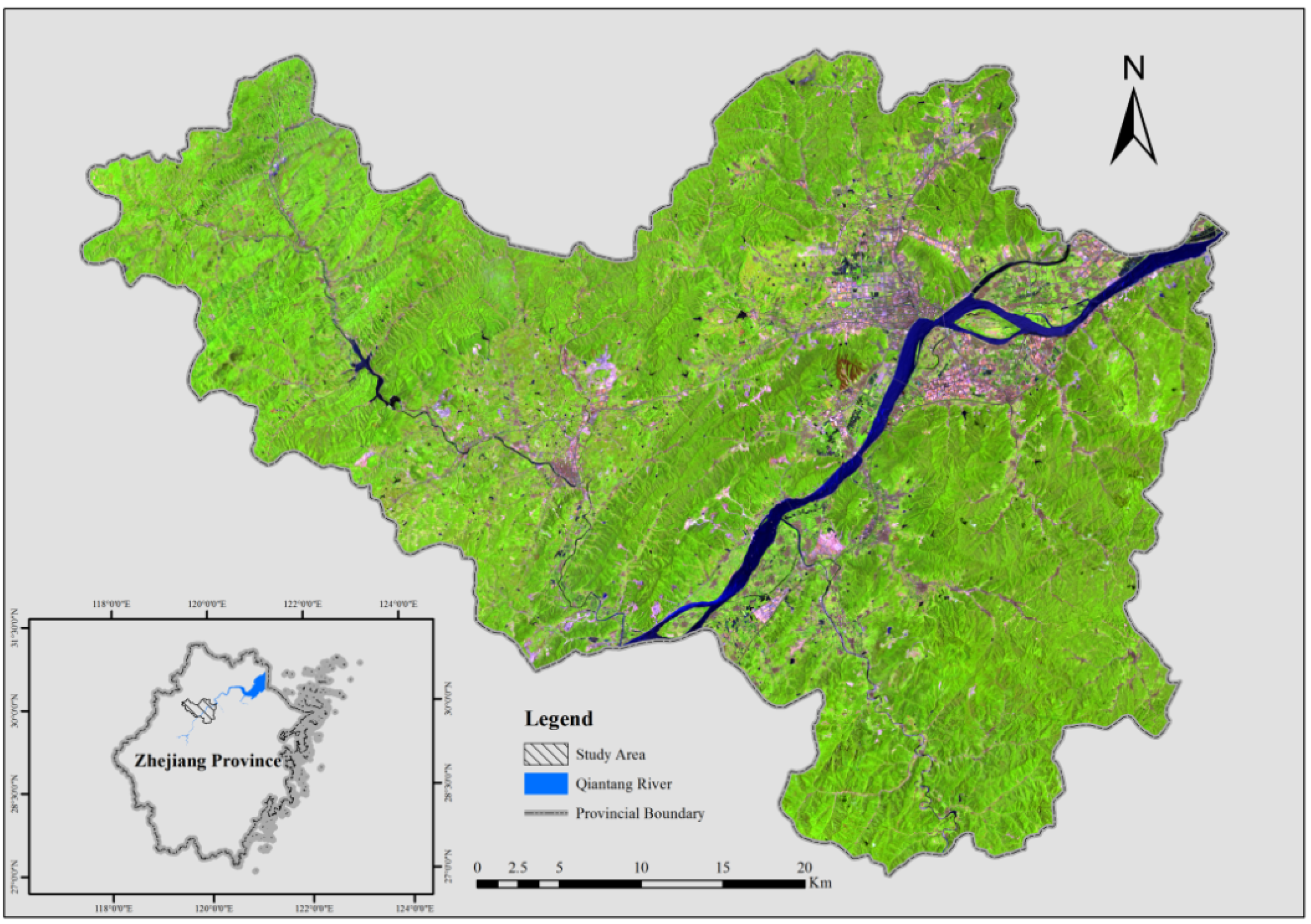
2.1. Study Area

The study area, Fuyang County, is located between Latitude 29°44′45″–30°11′58.5″N and Longitude 119°25′00″–120°19′30″E in Northwest Zhejiang Province, China, with about 71% of the land covered by forest, and is approximately 38 kilometers away from the capital city, Hangzhou. The prevailing waters include the Fuchun River, with several tributaries running across the region, and the Yanshi Ridge reservoir situated in the west (Figure 1). The area is characterized as a subtropical monsoon climate with an annual average precipitation of 1441.9 mm and a mean temperature of 16.1°C. The altitude varies from 1.6 m to 1063.4 m, and the land is predominantly covered with red soil and paddy soil. Coniferous forest (Pinus massoniana and Cunninghamia lanceolata), broadleaf forest (Lauraceae), mixed forest, bamboo (Phyllostachys pubescens), and shrub are the dominant forest species, as the primeval forests have almost been exhausted as historic consumption yielded to economical development; most of current forests are secondary vegetation [20].

Figure 1. The location of study area with Landsat image in 2013 (RGB: 543).

Figure 1. The location of study area with Landsat image in 2013 (RGB: 543).

2.2. Field Measurement

Field work is the foundation for remote sensing technology to extend limited stand information to large scale predictions. The two datasets used in this study are part of the field investigation data for Zhejiang Province, through a stratified random sampling approach using the same strategy in 2008 and 2013 administered by Zhejiang Forestry Academy. The allocation of hierarchical sample plots is based on a comprehensive consideration of geographical conditions and forest properties, including climate zone, tree species, age composition, and site characteristics. The theory of errors is employed to assure the quantity of typical samples, both in training and validation. The size of each inventory plot is 20 m × 20 m for trees, with three 2 m × 2 m subplots set in the diagonal line of each plot for shrubs and grasslands. Fundamental measurements are comprised of diameter at breast height (DBH), height and species recorded with Global Positioning System (GPS). The total Above Ground Biomass is the sum of tree, shrub, and herbaceous in each plot regarded and is as the final AGB with a unified unit of ton/ha. In general, six groups, including broadleaved forest, coniferous and broadleaved mixed forest, Shrub, Bamboo forest, Pine forest and Chinese fir forest, were calculated using specific allometric equations as a function of tree height and DBH, described in [21]. Main specific species included pine forest, Chinese fir, hardwood (I and II), Phyllostachys heterocycla cv. Pubescens, and so on. As the formulations developed by Yuan et al. have been successfully utilized to several provincial applications [22,23,24], we adopted those calculations for establishing aboveground biomass of sample plots. There are 87 and 80 sample plots for 2008 and 2013, respectively (Table 1).

Table 1. Statistics of field-based aboveground biomass.

Years	# Plots	Min AGB (ton/ha)	Max AGB (ton/ha)	Mean AGB (ton/ha)	Std.Dev.AGB (ton/ha)
2008	87	8.05291	193.2647	86.1533	40.76886446
2013	80	14.70901	219.692	98.7338	47.8469626

Table 1. Statistics of field-based aboveground biomass.

Years	# Plots	Min AGB (ton/ha)	Max AGB (ton/ha)	Mean AGB (ton/ha)	Std.Dev.AGB (ton/ha)
2008	87	8.05291	193.2647	86.1533	40.76886446
2013	80	14.70901	219.692	98.7338	47.8469626

2.3. Remote Sensing Data Pre-Processing

As mentioned above, Landsat imagery was chosen as the main remote sensing data source for its convenient procurability and suitable spectral information. To overcome the limited availability of cloud-free images, two Landsat Thematic Mapper (TM) 5 images and one Landsat Operational Land Imager (OLI) image (path/row: 119/39), with the least clouds, were selected as the data sources from the United States Geological Survey (USGS) website [25]. The standard level-one terrain-corrected L1T images geometrically calibrated and orthorectified to WGS-84 datum were acquired on different dates: 26 July 2004, 5 July 2008 and 19 July 2013. The images were obtained within the same month to minimize phonological influence. Visible bands and shortwave infrared bands were used as the spectral variables (except for the first blue band in 2013), and the thermal infrared channels were abandoned because of their coarser spatial resolution, both for TM and OLI. Radiometric calibration converting DN values to the top of the atmosphere radiance was conducted via the gain and offset information within the attached metadata files. Afterwards, atmospheric correction was completed by “Fast Line of sight Atmospheric Analysis of Spectral Hypercubes” (FLAASH) in ENVI software for the base image in 2008 [26], input parameters, including sensor type, flight time, atmospheric model, aerosol mode, and other parameters, were determined. Pseudo-Invariant Features (PIFs) were selected as the relative radiometric calibration method to make the 2004 and 2013 images consistent with the reference image from 2008 [27]; dark pixels located in water area and light pixels lay in roads, buildings were visually inspected and selected as invariant target pixels by referring to high resolution images and local knowledge to formulate the relationships between reference image and images to be corrected. SCS+C correction was executed to reduce topographical effect with the same resolution Digital elevation model (DEM) data [28], which would alleviate the overcorrection problem in sun-canopy-sensor (SCS) model by introducing adjustment coefficient analogous to C-correction. Here is the formulation:

$${\mathsf{\rho }}_{\mathrm{n}}=\mathsf{\rho }\times \frac{\cos \mathsf{\alpha }\times \cos \mathsf{\theta }+\mathrm{C}}{\cos \mathrm{i}+\mathrm{C}}$$

(1)

where ${\mathsf{\rho }}_{\mathrm{n}}$ is the objective reflectance, $\mathsf{\rho }$ is the uncorrected reflectance, $\mathsf{\alpha }$ is the terrain slope, $\mathsf{\theta }$ is the solar zenith angle, $\text{i}$ is the incidence angle, while $\cos \mathrm{i}$ and c are defined as follows:

$$\cos \mathrm{i}=\cos \mathsf{\alpha }\times \cos \mathsf{\beta }+\sin \mathsf{\alpha }\times \sin \mathsf{\theta }\times \cos \left(\mathsf{\phi }-\mathsf{\beta }\right)$$

(2)

where $\mathsf{\beta }$ is the terrain aspect and $\mathsf{\phi }$ is the solar azimuth angle. Besides, $\mathrm{C}$ is calculated as the ratio of $\mathrm{a}$ to $\mathrm{b}$, where $\text{a}$ means the regression slope and $\text{b}$ refers to the intercept.

$$\mathsf{\rho }=\mathrm{a}+\mathrm{b}\times \cos \mathrm{i}$$

(3)

2.4. Variables Derivation

One key procedure to build and apply the relationship between remote sensing data and forest biophysical property for biomass estimation is to extract valuable candidate Landsat derivations. By referring to previous studies, apart from the original multi-spectral bands, other potentially helpful variables from the processed Landsat image were calculated. Vegetation indices were proposed as preferably important measures for forest biophysical researches. Among the vegetation indices, Normalized Difference Vegetation Index (NDVI) is the most widely used index, however, in the present study, we adopted the improved index named NDVIc as we found that it had a stronger relationship with AGB because it combined the information of shortwave infrared band, which provides valuable information to biomass retrieval [29].

The NDVIc is defined as follows:

$${\text{NDVI}}_{\mathrm{C}}=\frac{\text{NIR}-\text{RED}}{\text{NIR}+\text{RED}}\times \left[1-\frac{\left(\text{MIR}-{\text{MIR}}_{\text{min}}\right)}{({\text{MIR}}_{\text{max}}-{\text{MIR}}_{\text{min}})}\right]$$

(4)

where NIR is the near-infrared band RED is the red band, MIR is the shortwave infrared band, MIR_max and MIR_min are values in the shortwave infrared band from closed canopies and open canopies. In this study, the last two values were extracted from the shortwave infrared band within the forest area for the highest value and the lowest value.

Tasseled Cap (TC) transformation was executed to reduce the primary multi-spectral information into reduced compendious features sensitive to vegetation characteristics, viz. brightness, greenness, and wetness [30]. Texture information was derived from the most practical method Gray Level Co-occurrence Matrix (GLCM), eight measurements including mean, variance, homogeneity, contrast, dissimilarity, entropy, second moment and correlation that were calculated from four bands (band2, band3, band4 and band5) with a window size of 3 × 3 pixels [31]. Moreover, DEM was used to generate topographical variables including slope, aspect and elevation.

In addition, the contemporaneous local Land Use and Cover maps were used as the reference to mask the non-forest area for three years to ensure that the modeling process was restricted to the forest area. Considering the positional uncertainties in GPS recordings, 3 × 3 pixels windows were used to calculate the mean values of remote sensing variables in the corresponding images.

2.5. Modeling Methods and Precision Assessment

To inspect the relationship between biomass and remote sensing variables, the field-measured AGB was considered as a dependent variable and imagery generated variables were treated as independent variables. Random forest algorithm was employed for regression as it showed significantly commendable performance than other regression techniques by previous studies and has been widely applied to environmental monitoring [32,33]. In this algorithm, numbers of decision trees are generated to the maximum extent without pruning by randomly selected two thirds of the data as training samples with bootstrapping, strengthening the flexibility by aggregating multiple classification and regression trees, and the remaining one third of data, also called out-of-bag (OOB), is used as validation samples to estimate the modeling errors. Furthermore, at each node of the decision tree, the selection of features for modeling is also stochastic, which makes the approach immune to the problem of over-fitting [34]. Therefore, there are two important parameters, respectively named mtry, denoted as the number of features used to split the nodes, and ntree, which means the number of trees to be adjusted to achieve a desirable prediction. Another advantage of the random forest algorithm is that it accomplishes excellent feature selection by automatically ranking the relative importance of variables. There are two mechanics in this algorithm to evaluate the importance of input variables, i.e., mean decrease in accuracy that assesses the effect of a variable, whether it makes the mean decrease in accuracy and mean decrease in Gini Index that infer the impurity of a variable. Taking this into account, all the remote sensing generated variables were used for AGB estimation, and the mean decrease in accuracy measure was used for noting the variables’ importance. The regression process was completed in the open access R statistical software [35] using the “randomForest” package [36]. The parameters mtry was set to the default value, one third of the total variables, and ntree was tested in the range of (100, 500, 800, 1000, 1500).

On account of the limited sample plots, 10-fold cross validation was employed to assess the estimated AGB performance during the modeling process. In addition, validation measures, including coefficient of determination (R²), Root Mean Squared Error (RMSE) between simulated AGB, and field measured biomass, were calculated to assess the estimation performance.

3. Results

3.1. Variable Importance for Modeling

The features adopted in the random forest regression for two years are shown in Figure 2. Non-parametric analysis Spearman’s rank correlation was also performed to assess the correlations between field-based measured AGB and remote sensing variables. As a result, multi-spectral bands, including band4, band5, band7, and texture measurements, including b5_mean, b4_mean, as well as TC components wetness and brightness, were selected as the top 10 important features, both in 2008 and 2013 random forest retrievals, which was in accordance with the Spearman’s rank correlation result (Table 2). Furthermore, the short wave infrared bands had a higher correlation coefficient in all strategies, which was consistent with previous studies [37]. In addition, the variable wetness presenting the moisture content was in high correlation with AGB, which may be owing to the primary water conservation forest occupying the majority in the Fuchun River watershed. However, there was some difference between the important variable selection results of random forest and Spearman’s rank correlation. Although some fluctuations may appear in the RF algorithm, it should be pointed out that some variables, not selected by the Spearman analysis, still played important roles in the estimation process.

Figure 2. The top 10 variables selected in random forest in 2008 and 2013.

Figure 2. The top 10 variables selected in random forest in 2008 and 2013.

Table 2. Variable selection result of Spearman’s rank correlation.

CorrelativeVariables in 2008		CorrelativeVariables in 2013
band7	−0.514 **	band7	−0.566 **
b5_mean	−0.499 **	b5_mean	−0.539 **
wetness	0.483 **	b4_mean	−0.539 **
band5	−0.480 **	wetness	0.509 **
brightness	−0.460 **	band5	−0.493 **
b4_mean	−0.439 **	band2	−0.386 **
band4	−0.413 **	brightness	−0.376 **
ndvic	0.397 **	b2_mean	−0.369 **
greenness	−0.396 **	band3	−0.363 **
band2	−0.372 **	band4	−0.262 *
b4_contrast	−0.285 **	band1	−0.240 *
band3	−0.284 **	b2_second moment	0.235 *
b2_mean	−0.278 **	b2_entropy	−0.228 *
b4_dissimilarity	−0.248 *
b3_mean	−0.232 *

Note: * Significant at a 0.05 level; ** Significant at a 0.01 level.

Table 2. Variable selection result of Spearman’s rank correlation.

CorrelativeVariables in 2008		CorrelativeVariables in 2013
band7	−0.514 **	band7	−0.566 **
b5_mean	−0.499 **	b5_mean	−0.539 **
wetness	0.483 **	b4_mean	−0.539 **
band5	−0.480 **	wetness	0.509 **
brightness	−0.460 **	band5	−0.493 **
b4_mean	−0.439 **	band2	−0.386 **
band4	−0.413 **	brightness	−0.376 **
ndvic	0.397 **	b2_mean	−0.369 **
greenness	−0.396 **	band3	−0.363 **
band2	−0.372 **	band4	−0.262 *
b4_contrast	−0.285 **	band1	−0.240 *
band3	−0.284 **	b2_second moment	0.235 *
b2_mean	−0.278 **	b2_entropy	−0.228 *
b4_dissimilarity	−0.248 *
b3_mean	−0.232 *

Note: * Significant at a 0.05 level; ** Significant at a 0.01 level.

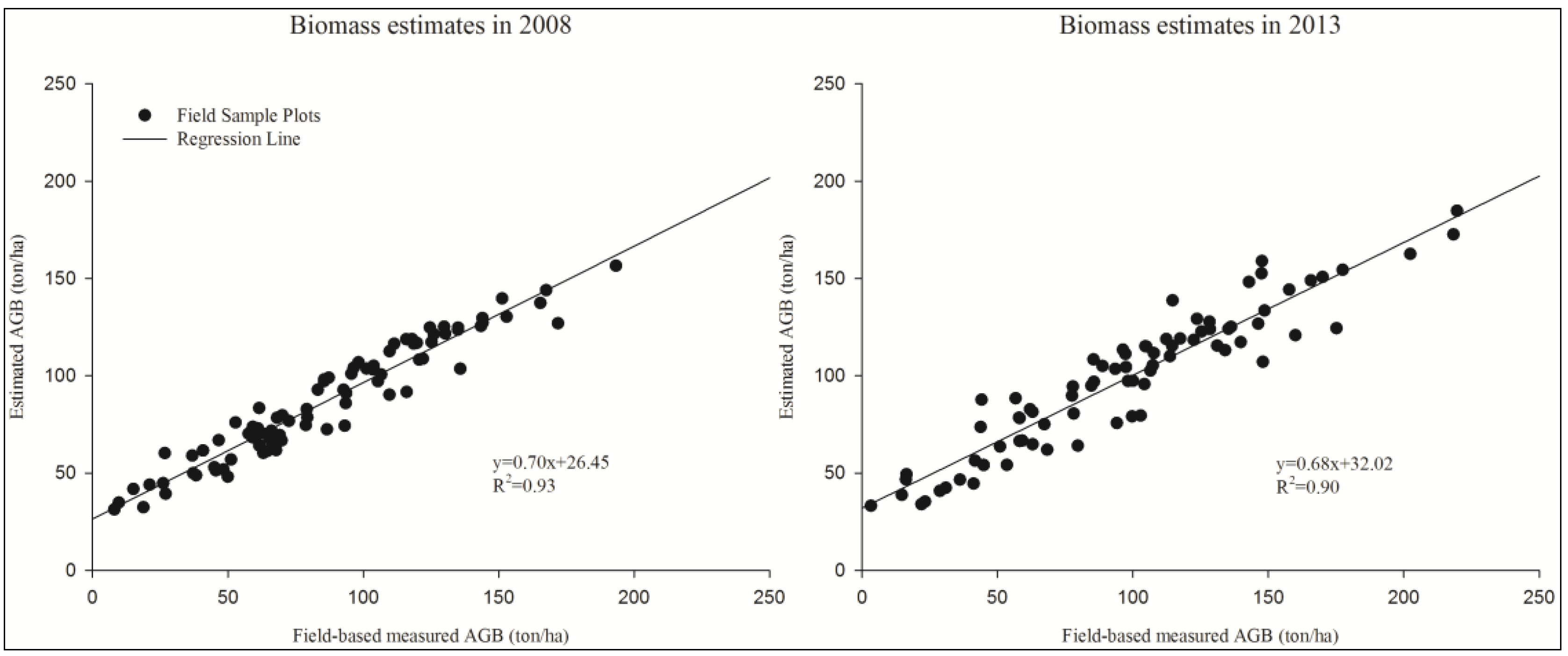
3.2. Accuracy Assessment

In the light of inevitable fluctuations in the random forest algorithm as the initial samples are randomly selected, the model processes in both years were repeated 20 times to acquire the mean values in the R statistical package, where the imputations were stabilized with the ntree value of 1000. Figure 3 shows the linear relationships between the estimated AGB and the field-based measured AGB, with a value of R² 0.93 and RMSE 11.16 ton/ha in 2008, and R² 0.90 and RMSE 16.9 ton/ha in 2013 (p value < 0.01). The results indicated that random forest, in two years, had an acceptable performance for AGB estimates. This may due to some of the following reasons: the number of plot samples used in the present study is limited with a selection of keeping homogeneous plots, while discarding the outliers using the 3 σ (standard deviation) measurement in both years; stochastic decisions in bootstrap sampling through out-of-bag error estimation, random variable selection, and taking both predictor and response variables into account, simultaneously, make the simulation effective; there are no assumptions about the population of sample plots and the relationships between Landsat image derivations and AGB for random forest regression, which is adaptive to complex forest characteristics. Nevertheless, it should be pointed out that the phenomena that the values of highest biomass were underestimated and the values of lowest biomass were overestimated still exists, as the result in random forest for regression adopts the mean values of predictions.

Figure 3. The relationship between estimated AGB and field-based measured AGB.

Figure 3. The relationship between estimated AGB and field-based measured AGB.

In addition, as it is usually difficult to investigate historical biomass information in practice, previous researches recommended that the same model could be applied to time series images which lack synchronous field data but corrected using relative corrections [38], therefore the identical random forest regression model adopted in the 2008 image was employed to the relatively corrected image in 2004 to generate an estimated AGB map. In addition, the AGB map in 2013 was generated separately, based on a random forest simulation using the simultaneous field-based data.

3.3. Aboveground Biomass Estimates

3.3.1. AGB Distribution Characteristic

The estimated AGB maps of three years in Fuyang County are shown in Figure 4. The mean values of AGB were 74.24 ton/ha, 76.33 ton/ha, and 99.63 ton/ha in 2004, 2008, and 2013, respectively, showing a significant rising trend in the past decades, owning to the measures that the government has taken in order to improve forest quality, such as young forest management and forest cultivation. Similar AGB distribution patterns were observed over the three periods, from the map that high-value biomass locations were lying close to the Fuchun River, where cultivated with broadleaf and coniferous forest. While relatively lower biomass positions were primarily distributed in the northwest, which was mostly planted with shrubs and some plantations for timber production. The primary forest around the Yanshi Ridge reservoir was highwood, according to the local Land Use and Land Cover map. Furthermore, in the southeast of the study area, as the majority of natural secondary forests were planted with phyllostachys pubescens, when compared to broadleaf and coniferous forest, the bamboo forest had a relatively lower biomass value. The discrepancies of AGB estimation distribution were similar to the distinct arrangement characteristic of different forest species, reflecting that the local tripartite programming had a great influence on forest allocation and development.

Figure 4. Estimated aboveground biomass in Fuyang County over three periods.

Figure 4. Estimated aboveground biomass in Fuyang County over three periods.

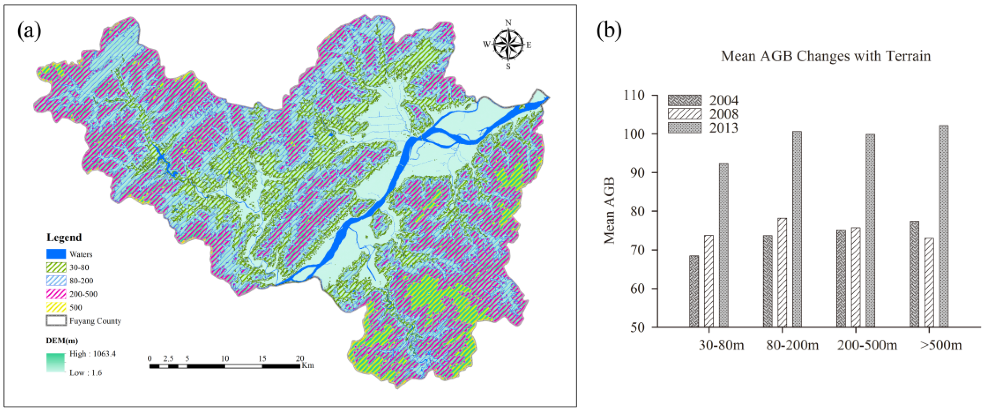
3.3.2. AGB Changes with Terrain

As the main soil type in the study area was red soil that mainly distributed across an elevation of 200–500 m, the terrain was divided into four stratifications (Figure 5a) to investigate the mean value of AGB change among different elevation gradients. Because temperature, precipitation and other environmental factors vary with elevation, the estimated biomass exhibits non-stationary biomass variations in terms of altitude. With the increase of elevation, the mean value of biomass was gradually increased in the three years, except in 2008, which may have been greatly influenced by the freezing rain and snow disaster at the beginning of that year, the biomass even decreased with higher elevation. Additionally, the greatest increase rate 36.46% took place in the 80–200 m gradation from 2004 to 2013, followed by the 30–80 m gradation (34.88%), when compared to the growth above 200-m elevations (30.93%).

Figure 5. (a) Map of elevation stratification, and (b) change of AGB with stratified terrain.

Figure 5. (a) Map of elevation stratification, and (b) change of AGB with stratified terrain.

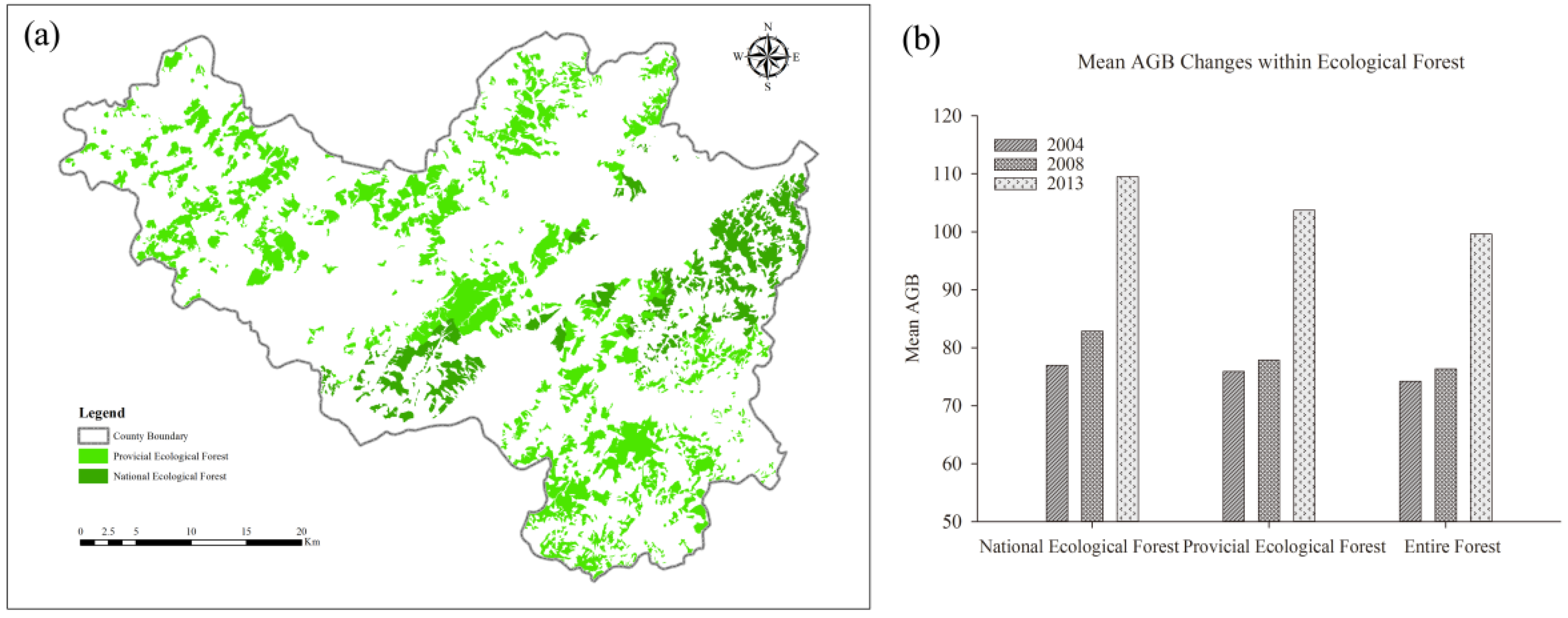
3.3.3. AGB Change within Ecological Forest

The outcome in Figure 6 illustrates that the AGB spatial distribution exhibited different characteristics within two level ecological forests. In general, the mean value of AGB within the national ecological forest was higher than that located in the provincial ecological forest over all the periods, which conforms to the original design that national ecological forest possesses the highest susceptible location and occupied the most important geographic niches. Furthermore, AGB values in these two ecological forests were higher than that of the contemporaneous entire forest, suggesting that the established ecological forest delineation has a greater potential for local carbon sink and carbon storage. Meanwhile, the increase rate values of AGB in national ecological forest, provincial ecological forest and normal forest were 42.26%, 36.65%, and 32.19%, respectively, indicating that the policy of establishing ecological forest showed an obvious positive effect on forest ecosystem protection.

Figure 6. (a) Map of two-level ecological forest, and (b) change of AGB within ecological forest.

Figure 6. (a) Map of two-level ecological forest, and (b) change of AGB within ecological forest.

4. Discussion

4.1. Reasons for AGB Changes

The reason to explain the overall increase biomass with regard to the terrain over the past decade may be due to the measurements taken by the local government. For example, in recent years, forest ecosystems along the Fuchun River banks and tributaries about 9600 hectare at low altitude were preserved with an emphasis on rebuilding zonal ecological protection forests to improve environment quality. Moreover, afforestation in the flat-land areas was promoted by changing part of cultivated land to forest along with implementing plantations to be tree-lined [20]. For mountain areas, more forest parks and nature reserves were established through enclosing the hills for natural reforestation. Figure 5b indicates the powerful restorative capability recovered from natural disasters with distinct biomass augments. Nevertheless, when the practicality is taken into consideration, geographic limitations, such as transportation convenience and water availability, areas located in higher elevations were less affected by human activities than the lower mountain areas, which may explain the phenomenon that regions located in heights below 200 m displayed larger AGB increases. However, it should be noted that effective measurements, planned to improve the forest quality, are supposed to balance natural conditions and socioeconomic development.

On the other hand, the implementation of ecological forest suggested significantly positive effects on biomass distribution and improvement. Since 2001, the government in Zhejiang Province had delimited about 197.1 × 104 hm² of forest (accounting for 29.43% of the forest region) as ecological forests, also named public welfare forests, which are mainly distributed in river headwaters, river banks, large reservoirs, natural reserves and famous scenery, where presents high ecological significance and low ecological vulnerability, in order to separate them from the commercial forests through different operation and management patterns. As to the implementation in Fuyang County, 423.73 km² area of forests were delimited as key ecological forests, of which national-level ecological forest occupied 104.27 km² and provincial-level took up 319.46 km², in total accounting for 37.83% of the entire forest. They are mainly distributed along the Fuchun River basin and national highways, reservoir, as well as scenic spots and forest parks. According to the official gazette on Fuyang key ecological forest, published in 2014, analogous to the research on riparian forests mentioned by [39], the maximal ecological benefit is for water conservation, which was evaluated to count for 56.09 billion Yuan when referring to the local Environmental Bulletin. To attract more attention of the public and to improve the awareness of ecological forest protection, the compensation funds have been gradually increased from the original 8 Yuan/mu to 30 Yuan/mu. All these measurements have promoted local forest conservation, which is reflected by the biomass increase.

4.2. Uncertainty Analysis

The reason that subspecies were not distinguished in this study, except for the limited number of sample plots, was that we wanted to accomplish recapitulative biomass estimation at the regional scale. The mean AGB for the ecological forest is 106.61 ton/ha and 99.63 ton/ha for the entire forest, compared to previous research utilizing field inventory data in Zhejiang Province. Qian et al. [40] predicted the mean biomass of ecological forests in the whole province would increase to 99.30 t·hm⁻² in 2011, and Zhang et al. [22] mentioned that the mean biomass forest in Xianju County was 94.51 t·hm⁻² in 2008. Other than the study conducted by Chen [41], obtaining a result of 113.33 t·hm⁻² for the Liandu District ecological forest in 2008, which exhibited a higher value than our result, the others showed comparable estimates with this study.

A great deal of uncertainty still exists when estimating forest biomass [42]. Strictly speaking, complete biomass is comprised of above-ground and under-ground components, while we only focused on the above-ground biomass as the main objective. Optical imagery has obvious limitations for AGB estimates, for instance, the backgrounds, including understory vegetation and soil, can greatly influence the relationship between AGB and derived spectral bands. The spectral information is representative of tree canopy, but defective for the three-dimensional properties of the forest [43]. All this suggests that there exist gaps, but potential improvement for accuracy biomass retrieval. Since remote sensing has the advantage of macroscopic and dynamic monitoring, it provides powerful specific spectral change information and linked relationships to forest biophysical properties to investigate the interactions between environmental variables and human activities. Biomass distribution and change were simulated in the present study to quantify human activities’ effects on forest ecosystems, revealing corresponding intensive biomass reactions to human interventions. Consequently, multi-source images containing more tree parameter information, associated with systematic forest administration, will be considered for further research in order to achieve more precise observations.

5. Conclusions

Remote sensing provides nondestructive and continues detection information on biomass of forest ecosystem. With the open access of Landsat imagery and rapid development of computer science, especially machine learning approaches, time-series remote sensing records could be applied to an AGB investigation, not only expanding the traditional, limited plot scale to regional or larger spatial scales, but also increasing temporal acquisitions of biomass dynamics with lower cost and higher efficiency. The economic, modern techniques, cooperating with field-based survey, helps to gain a better understanding of the interactions between human activities and forest properties in a spatially macroscopical perspective, which would present vegetation evolution processes and illuminate subsequent policy decisions.

In this study, Landsat image and field data were integrated to estimate the three period forest aboveground biomass in Fuyang County, Zhejiang Province, China, using the random forest regression with a reliable R² above 0.9, and RMSE below 12 ton/ha. The results showed that the estimated AGB increased distinctly from the mean value of 74.24 ton/ha in 2004 to 99.63 ton/ha in 2013, and the spatial pattern of the predicted AGB, primarily dominated by plantations, presented a close relationship with geomorphology and human behavior, dominated by local forest management. In summary, anthropological activities, including afforestation and other forest protection projects, particularly available below 200-m elevation, in conjunction with ecological forest delimitation, especially within the national level ecological forest, greatly influenced the distribution and change of forest AGB, which indicates that Landsat imagery-based AGB estimates would provide valuable information to better understand the forest ecosystem and promote sustainable development.

References

1. Costanza, R.; D’Arge, R.; de Groot, R.; Farber, S.; Grasso, M.; Hannon, B.; Limburg, K.; Naeem, S.; O’Neill, R.V.; Paruelo, J.; et al. The value of the world’s ecosystem services and natural capital. Ecol. Econ. 1998, 25, 3–15. [Google Scholar] [CrossRef]
2. Liu, J.; Dietz, T.; Carpenter, S.R.; Alberti, M.; Folke, C.; Moran, E.; Pell, A.N.; Deadman, P.; Kratz, T.; Lubchenco, J.; et al. Complexity of coupled human and natural systems. Science 2007, 317, 1513–1516. [Google Scholar] [CrossRef] [PubMed]
3. Olander, L.P.; Gibbs, H.K.; Steininger, M.; Swenson, J.J.; Murray, B.C. Reference scenarios for deforestation and forest degradation in support of REDD: A review of data and methods. Environ. Res. Lett. 2008. [Google Scholar] [CrossRef]
4. Zhang, G.; Ganguly, S.; Nemani, R.R.; White, M.A.; Milesi, C.; Hashimoto, H.; Wang, W.; Saatchi, S.; Yu, Y.; Myneni, R.B. Estimation of forest aboveground biomass in California using canopy height and leaf area index estimated from satellite data. Remote Sens. Environ. 2014, 151, 44–56. [Google Scholar] [CrossRef]
5. Zheng, S.; Cao, C.; Dang, Y.; Xiang, H.; Zhao, J.; Zhang, Y.; Wang, X.; Guo, H. Retrieval of forest growing stock volume by two different methods using Landsat TM images. Int. J. Remote Sens. 2014, 35, 29–43. [Google Scholar] [CrossRef]
6. Wang, X.; Shao, G.; Chen, H.; Lewis, B.J.; Qi, G.; Yu, D.; Zhou, L.; Dai, L. An Application of Remote Sensing Data in Mapping Landscape-Level Forest Biomass for Monitoring the Effectiveness of Forest Policies in Northeastern China. Environ. Manag. 2013, 52, 612–620. [Google Scholar] [CrossRef] [PubMed]
7. Lu, D.; Chen, Q.; Wang, G.; Liu, L.; Li, G.; Moran, E. A survey of remote sensing-based aboveground biomass estimation methods in forest ecosystems. Int. J. Digit. Earth 2014. [Google Scholar] [CrossRef]
8. Du, L.; Zhou, T.; Zou, Z.; Zhao, X.; Huang, K.; Wu, H. Mapping Forest Biomass Using Remote Sensing and National Forest Inventory in China. Forests 2014, 5, 1267–1283. [Google Scholar] [CrossRef]
9. Roy, D.P.; Wulder, M.A.; Loveland, T.R.; Woodcock, C.E.; Allen, R.G.; Anderson, M.C.; Helder, D.; Irons, J.R.; Johnson, D.M.; Kennedy, R.; et al. Landsat-8: Science and product vision for terrestrial global change research. Remote Sens. Environ. 2014, 145, 154–172. [Google Scholar] [CrossRef]
10. Lu, D. The potential and challenge of remote sensing-based biomass estimation. Int. J. Remote Sens. 2006, 27, 1297–1328. [Google Scholar] [CrossRef]
11. Dube, T.; Mutanga, O. Evaluating the utility of the medium-spatial resolution Landsat 8 multispectral sensor in quantifying aboveground biomass in Mgeni catchment, South Africa. ISPRS J. Photogramm. Remote Sens. 2015, 101, 36–46. [Google Scholar] [CrossRef]
12. Zhu, X.; Liu, D. Improving forest aboveground biomass estimation using seasonal Landsat NDVI time-series. ISPRS J. Photogramm. Remote Sens. 2015, 102, 222–231. [Google Scholar] [CrossRef]
13. Pflugmacher, D.; Cohen, W.B.; Kennedy, R.E.; Yang, Z. Using Landsat-derived disturbance and recovery history and lidar to map forest biomass dynamics. Remote Sens. Environ. 2014, 151, 124–137. [Google Scholar] [CrossRef]
14. Liu, Q.; Yang, L.; Liu, Q.; Li, J. Review of forest above ground biomass inversion methods based on remote sensing technology. J. Remote Sens. 2015, 19, 62–74. [Google Scholar]
15. Latifi, H.; Nothdurft, A.; Koch, B. Non-parametric prediction and mapping of standing timber volume and biomass in a temperate forest: Application of multiple optical/LiDAR-derived predictors. Forestry 2010, 83, 395–407. [Google Scholar] [CrossRef]
16. Güneralp, İ.; Filippi, A.M.; Randall, J. Estimation of floodplain aboveground biomass using multispectral remote sensing and nonparametric modeling. Int. J. Appl. Earth Obs. Geoinform. 2014, 33, 119–126. [Google Scholar] [CrossRef]
17. Fu, W.; Fu, Z.; Ge, H.; Ji, B.; Jiang, P.; Li, Y.; Wu, J.; Zhao, K. Spatial Variation of Biomass Carbon Density in a Subtropical Region of Southeastern China. Forests 2015, 6, 1966–1981. [Google Scholar] [CrossRef]
18. Liu, L.; Peng, D.; Wang, Z.; Hu, Y. Improving artificial forest biomass estimates using afforestation age information from time series Landsat stacks. Environ. Monit. Assess. 2014, 186, 7293–7306. [Google Scholar] [CrossRef] [PubMed]
19. Liu, C.; Zhang, L.; Li, F.; Jin, X. Spatial modeling of the carbon stock of forest trees in Heilongjiang Province, China. J. For. Res. 2014, 25, 269–280. [Google Scholar] [CrossRef]
20. Qiu, L.; Zhu, J.; Wang, K.; Hu, W. Land Use Changes Induced County-Scale Carbon Consequences in Southeast China 1979–2020, Evidence from Fuyang, Zhejiang Province. Sustainability 2015. [Google Scholar] [CrossRef]
21. Yuan, W.; Jiang, B.; Ge, Y.; Zhu, J.; Shen, A. Study on Biomass Model of Key Ecological Forest in Zhejiang Province. J. Zhejiang For. Sci. Technol. 2009, 29, 1–5. [Google Scholar]
22. Zhang, J.; Gao, H.; Ying, B.; Wang, J.; Yuan, W.; Zhu, J.; Yi, L.; Jiang, B. The biomass dynamic analysis of public walfare forest in Xianju county of Zhejiang province. J. Nanjing For. Univ. Nat. Sci. Ed. 2011, 35, 147–150. [Google Scholar]
23. Du, Q.; Xu, J.; Wang, J.; Zhang, F.; Ji, B. Correlation between forest carbon distribution and terrain elements of altitude and slope. J. Zhejiang AF. Univ. 2013, 30, 330–335. [Google Scholar]
24. Qian, Y.; Yilita; Dou, P.; Zhu, G.; Ying, B.; Yu, S. Biomass and carbon fixation with oxygen release benefits in an ecological service forest of Jinyun County, China. J. Zhejiang AF. Univ. 2012, 29, 257–264. [Google Scholar]
25. U.S. Geological Survey. Available online: http://glovis.usgs.gov (accessed on 20 July 2015).
26. Cooley, T.; Anderson, G.P.; Felde, G.W.; Hoke, M.L.; Ratkowski, A.J.; Chetwynd, J.H.; Gardner, J.A.; Adler-Golden, S.M.; Matthew, M.W.; Berk, A.; et al. FLAASH, a MODTRAN4-based atmospheric correction algorithm, its application and validation. In Proceedings of the IEEE International Symposium on Geoscience and Remote Sensing (IGARSS), Munich, Germany, 24–28 June 2002; pp. 1414–1418.
27. Myeong, S.; Nowak, D.J.; Duggin, M.J. A temporal analysis of urban forest carbon storage using remote sensing. Remote Sens. Environ. 2006, 101, 277–282. [Google Scholar] [CrossRef]
28. Soenen, S.A.; Peddle, D.R.; Coburn, C.A. SCS+C: A modified Sun-canopy-sensor topographic correction in forested terrain. IEEE Trans. Geosci. Remote Sens. 2005, 43, 2148–2159. [Google Scholar] [CrossRef]
29. Nemani, R.; Pierce, L.; Running, S.; Band, L. Forest ecosystem processes at the watershed scale—Sensitivity to remotely-sensed leaf-area index estimates. Int. J. Remote Sens. 1993, 14, 2519–2534. [Google Scholar] [CrossRef]
30. Crist, E.P.; Cicone, R.C. A physically-based transformation of Thematic Mapper data—The TM Tasseled Cap. IEEE Trans. Geosci. Remote Sens. 1984, 22, 256–263. [Google Scholar] [CrossRef]
31. Dube, T.; Mutanga, O. Investigating the robustness of the new Landsat-8 Operational Land Imager derived texture metrics in estimating plantation forest aboveground biomass in resource constrained areas. ISPRS J. Photogramm. Remote Sens. 2015, 108, 12–32. [Google Scholar] [CrossRef]
32. Zhang, J.; Huang, S.; Hogg, E.H.; Lieffers, V.; Qin, Y.; He, F. Estimating spatial variation in Alberta forest biomass from a combination of forest inventory and remote sensing data. Bio. Geosci. 2014, 11, 2793–2808. [Google Scholar] [CrossRef] [Green Version]
33. Kwon, Y.; Li, F.; Chung, N.; Bae, M.; Hwang, S.; Byoen, M.; Park, S.; Park, Y. Response of Fish Communities to Various Environmental Variables across Multiple Spatial Scales. Int. J. Environ. Res. Public Health 2012, 9, 3629–3653. [Google Scholar] [CrossRef] [PubMed]
34. Breiman, L. Random forests. Mach. Learn. 2001, 45, 5–32. [Google Scholar] [CrossRef]
35. R Core Team. R: A Language and Environment for Statistical Computing. R Foundation for Statistical Computing. Available online: http://www.R-project.org/ (accessed on 20 September 2015).
36. R Core Team. R: A Language and Environment for Statistical Computing; R Foundation for Statistical Computing: Vienna, Austria, 2012. [Google Scholar]
37. Baccini, A.; Laporte, N.; Goetz, S.J.; Sun, M.; Dong, H. A first map of tropical Africa’s above-ground biomass derived from satellite imagery. Environ. Res. Lett. 2008. [Google Scholar] [CrossRef]
38. Lu, D.; Batistella, M. Exploring TM image texture and its relationships with biomass estimation in Rondônia, Brazilian Amazon. Acta Amazon. 2005, 35, 249–257. [Google Scholar] [CrossRef]
39. Clipp, H.; Anderson, J. Environmental and Anthropogenic Factors Influencing Salamanders in Riparian Forests: A Review. Forests 2014, 5, 2679–2702. [Google Scholar] [CrossRef]
40. Qian, Y.; Yi, L.; Zhang, C.; Yu, S.; Shen, L.; Peng, D.; Zheng, C. Biomass and Carbon Storage of Public Service Forests in the Central Area of Zhejiang Province. Sci. Silvae. Sin. 2013, 49, 17–23. [Google Scholar]
41. Yan-fen, C. Dynamic analysis of Vegetation Biomass and Carbon Storage of Public Welfare Forests in Liandu District. J. Sichuan For. Sci. Technol. 2014, 35, 66–69. [Google Scholar]
42. Lu, D.; Chen, Q.; Wang, G.; Moran, E.; Batistella, M.; Zhang, M.; Vaglio Laurin, G.; Saah, D. Aboveground Forest Biomass Estimation with Landsat and LiDAR Data and Uncertainty Analysis of the Estimates. Int. J. For. Res. 2012. [Google Scholar] [CrossRef]
43. Ji, L.; Wylie, B.K.; Brown, D.R.N.; Peterson, B.; Alexander, H.D.; Mack, M.C.; Rover, J.; Waldrop, M.P.; McFarland, J.W.; Chen, X.; et al. Spatially explicit estimation of aboveground boreal forest biomass in the Yukon River Basin, Alaska. Int. J. Remote Sens. 2015, 36, 939–953. [Google Scholar] [CrossRef]