1. Introduction
The need to improve the energy efficiency of Europe’s building stock, which accounts for over 40% of the continent’s energy consumption, is increasingly pressing. Improving energy efficiency offers an opportunity to lower energy dependency and mitigate the effects of climate change [
1]. Numerous earlier studies on Spain’s residential sector identify the urban areas developed between the end of the Spanish Civil War and 1979 as inefficiency clusters located in the main cities of the country [
2,
3,
4,
5]. At present, most of the buildings constructed in these areas require huge amounts of energy to meet their occupants’ basic energy needs and, as such, are essentially enormous energy sinks [
6].
In many cases, these housing developments are located in low-income areas, meaning that the cost of the measures required may well be unaffordable for their residents [
7]. The reduction in energy costs achieved by heat insulation may not justify the investment, as the payback period may simply be too long for households suffering from energy poverty, in which reducing consumption comes at the cost of sacrificing material comfort [
8].
The deficiencies in the residential sector are a vector of discomfort, energy poverty and health problems for the occupants of inefficient buildings [
9], which could be addressed through envelope renovation [
10]. In Europe, a higher incidence of health problems (both physical and mental) was found among the population living in energy poverty [
11], which is most prevalent in southern and eastern European countries [
12]. In the case of Spain, studies analysing the impact of cold spells on mortality conclude that the excess deaths produced in winter are frequent in deprived neighbourhoods [
13]. Building envelope refurbishment is one of the tools used to reduce energy poverty and improve comfort levels in affected homes.
In order to cut final and primary energy consumption, improve comfort and reduce CO
2 and other pollutant emissions in cities, minimizing buildings’ energy demand is considered a priority. Furthermore, these measures entail a series of non-energy benefits that are not included in cost–benefit analyses but have a significant influence on safety, health and quality of life [
14].
Building stock currently holds enormous potential for improved energy efficiency that, as yet, remains untapped [
15]. Neighbourhood-scale retrofitting is less costly than tackling each building individually and offers local councils greater opportunities to apply energy and sustainability strategies [
16,
17,
18]. Key to overcoming the barriers these processes face are flexible urban planning, information transparency, strong support for public participation and attractive incentives to initiate the process. The affected population also needs to understand the issue [
19]. In order to ensure effective, fact-based communication, detailed preliminary studies that accurately determine which energy savings and improvements in comfort are achievable by energy retrofitting buildings are required [
20,
21].
To date, various building stock models have been constructed to estimate building energy consumption and that of the residential sector [
22,
23]. These are then used to calculate the benefits gained by investing in energy retrofitting [
15]. Some of these approaches are based on physical building energy simulation (BES) models (white box models) [
24,
25], others on measured data (black box models) and others on hybrid techniques (grey box models) [
26,
27,
28]. The latter reconciles the results produced by the models with real-world monitoring data with the aim of achieving more precise and reliable outcomes. This reconciliation of the model’s results with the measured data is known as calibration [
29].
The models for predicting the energy savings and CO
2 emission reductions achieved by measures to improve building stock energy efficiency are usually based on statistical data and energy simulations using standardized datasets (white box models) [
26]. The models based on data collection (black box models) compile information into categories of variables that influence energy performance [
30]. Recent research classified these variables into the following groups [
31]: meteorological information, indoor environmental quality information [
32,
33], occupancy-related data [
34,
35,
36,
37,
38], time indicators, building characteristics [
39], socio-economic information [
40] and historical data. The performance gap can only be bridged by adopting a broad and coordinated approach that includes the validation and verification of theoretical BES models [
41].
The Habita_RES project analyses the energy efficiency of Madrid’s residential buildings, focusing on those constructed on the outskirts of the city between 1940 and 1979 [
42]. Urban energy efficiency models were developed for existing residential buildings [
43], and several applications of monitoring methodologies [
44] made it possible to compare the models with real-world data. This paper presents a case study of building envelope retrofitting in the Manoteras district of Madrid. It draws on information about two very similar multi-occupant residential buildings, one that was refurbished and one that was not.
The overall objective of this paper is to develop methods, based on empirical and simulation data, with which to determine the energy saving achieved after energy retrofitting residential buildings representative of Madrid’s inefficient building stock. It aims to analyse in depth the possible differences between the energy savings estimated using residential building models and the real-world results measured in a series of specific cases. To this end, theoretical models are compared against data collected during monitoring [
45]. The initial hypothesis is that energy consumption is lower and comfort is greater in the retrofitted buildings. The intention of the assessment is to draw not only on energy consumption but also on experimental comfort and air quality data gathered by monitoring indoor environmental quality.
2. Case Study
The first social housing units in the Poblado Dirigido de Manoteras residential development were designed and built between 1958 and 1966. These new towns were conceived in the post-war era with the intention of applying the principles of architectural rationalism to contemporary social housing [
46]. They were intended to house the population that, largely as a consequence of the rural exodus following the Spanish Civil War, was living in the makeshift settlements that sprang up on the outskirts of the city [
47]. The project is an icon of modern architecture [
48] and was designed by architects Marino García Benito, Eduardo García Rodríguez and Enrique Quereizaeta Enríquez under the supervision of fellow architect Manuel Ambrós Escanellas [
49]. As was frequently the case in these developments, energy efficiency measures were not included, and none of the building envelope was insulated, resulting in extremely high heating demands [
50].
Figure 1 shows a heating demand model for all the residential buildings in the district, created using an urban assessment tool [
51] developed for the Habita_RES project [
42]. The model identifies the most inefficient buildings in which energy retrofitting should, therefore, be prioritized.
The case study was carried out on two five-storey residential buildings with two homes per floor. The buildings are adjoining and have east- and west-facing façades. Each building is constructed on a 142 m2 plot and has a gross floor area of 706 m2.
Figure 2 illustrates the case study buildings: the original building with exposed brickwork and the refurbished building with white cladding and yellow shading elements. The first is in its original state (OB) and has one south-facing side. The second building (retrofitted) has one north-facing side.
The refurbished block was retrofitted in April 2017 [
52]. The retrofitting included passive measures to improve the building envelope’s thermal performance (sides and roof) and a new solar protection system. The retrofitted building (RB) has a lattice system attached to the façade to provide solar protection and unify the building’s appearance. The advantage of this solar protection system is that it can be used as both awning and blind, allowing users to adjust it to their needs. The windows, heating and hot water systems were not upgraded as they are individual to each home and were not included in the improvements.
In the case of the refurbished building, the execution project incorporates the energy certification in both the state before (OB) and after the refurbishment works (RB) (
Table 1). The certificates were obtained using the simplified method employing the official tool CE3X.
3. Materials and Methods
The methodology consists of performing a series of complementary actions that make it possible to estimate the energy consumption of the buildings under study before (OB) and after refurbishing (RB) the building envelope. To this end, the buildings are modelled to calculate their theoretical energy consumption. This information is supplemented with monitored data recorded over the course of a year, and that includes information on energy consumption and indoor environmental quality. This provides a comprehensive dataset with which to evaluate the improvements obtained by retrofitting and analyse the discrepancies with the forecasts based on the simulation models [
53].
3.1. Construction of the Energy Simulation Model
Energy simulation models were developed from detailed information on the actual physical characteristics of each building. The information on the block in its original state was obtained from previous studies based on residential building samples [
5]. The characteristics of the refurbished building were obtained from the retrofitting project documents [
52]. To obtain simulation results that reflect the real-world situation as closely as possible, volumes representing the nearby urban environment were included. This makes it possible to consider both passive incident solar radiation on the building and the impact on the energy demand calculation of elements obstructing solar radiation. The thermal transmittance values for the walls were obtained using the regulatory method for calculating the parameters characteristic of the building envelope [
54], being the same as the information introduced in the simulation model. Thermal resistance was calculated using the homogeneous layer addition method (
Table 2). The energy simulations were performed with the Design Builder v6.1.8 software developed by Design Builder Software Ltd. (Stroud, UK) to evaluate new and existing buildings’ environmental performance. As simulation engine, Energy Plus (version 8.9), developed by the US Department of Energy (DoE), was used.
As a first approach to studying the buildings’ energy performance, their theoretical heating and cooling demands were calculated. This was performed using the parameters set for spaces destined for private residential use in Spain’s building code (Código Técnico de la Edificación; CTE [
55]) and building energy certification (Certificación Energética de Edificios [
56]) procedure. The main parameters employed in the baseline simulation are detailed below. Otherwise, in all the energy simulation models studied in this paper, the HVAC system was configured using the simple mode. In Design Builder, the Simple HVAC system is used during the early design phases or in analyses that require a basic treatment of the heating, cooling and mechanical ventilation systems (
Figure 3).
3.1.1. Climate Data
To establish the outdoor conditions contemplated in the calculation, the generic hourly climate data compiled as part of the documentation referred to in [
55] was used. These are the official data used to determine demand in the climate zone in which Madrid is located (D3).
In the calibration process, the 2020 hourly meteorological data, which are published monthly by Madrid City Council were used. The weather station selected for its proximity to the dwellings was number 107 (J.M.D. Hortaleza, located at Ctra. de Canillas, 2 [−3.656667, 40.462778]). The climate data used by Energy Plus (ESP_MADRID_IWEC.epw) were updated with the data provided by the weather station.
3.1.2. Internal Loads
The simulated buildings’ internal load is separated into three sources: occupants, equipment and lighting. As can be seen in
Table 3, the CTE considers the load (W/m
2) to be the same for both lighting and equipment.
3.1.3. Air Infiltration
To calculate the losses due to air infiltration, the values laid down in the CTE were used, these being 0.34 air changes per hour (ACH) for the OB and 0.25 ACH for the RB, the improvement in airtightness being considered a consequence of refurbishing the building envelope. The estimates were made according to the calculation criteria laid down in the regulatory document establishing the technical specifications for building energy performance assessment procedures (Condiciones técnicas de los procedimientos para la evaluación de la eficiencia energética de los edificios).
https://ecoeficiente.es/infiltracioneshe/ (accessed on 1 April 2024).
3.1.4. Mechanical and Natural Ventilation
According to the regulations, airflows within residential buildings must comply with the hygiene threshold of 0.63 ACH (outdoor air) per area, achieved using mechanical ventilation [
57]. The CTE also proposes using natural ventilation overnight during the summer in homes. The mechanical ventilation should be programmed to operate 24 h a day between October and May and from 08:00 to 23:00 between June and September. Meanwhile, natural ventilation should be used from 00:00 to 07:00 between June and September.
3.1.5. Heating and Cooling Systems
Climate control equipment configuration adheres to parameters outlined by local regulations. Specifically, it includes natural gas heating with an efficiency rating of 0.92 and electric cooling with an efficiency rating of 2.60.
As regards the retrofitting of the dwellings and calculation of the energy demand in terms of both heating (October to May) and cooling (June to September), the temperatures that the inhabited indoor spaces must reach are defined. As shown in
Table 4, the winter temperature settings are 17 °C overnight and 20 °C during the day. In summer, the temperature settings are 27 °C overnight and 25 °C during the day.
3.1.6. Solar Protection Systems
Another important aspect specified in the regulations is the impact of thermal gains due to the incidence of sunlight on external windows. Shading is, therefore, employed, programming deployment of systems protecting the openings in the façade from 08:00 to 24:00 between June and September. Reduction of energy losses when the heating systems are in operation is also addressed by shutting the blinds from 22:00 to 07:00 between October and May. Since the solar protection elements in both buildings are manually operated by the residents, this information was not initially available. Consequently, a decision was made to implement the programming mandated by regulations uniformly across all dwellings.
3.2. Monitoring of Energy Consumption and Indoor Environmental Quality
As part of the Habita_RES project, a monitoring system was installed in a sample of the homes in the two buildings [
42]. Monitoring was conducted over the course of a year (2020) and consisted of recording information on energy efficiency in five homes: two in the building in its original state and three in the refurbished building. The project also included installation of a weather station on the roof of one of the buildings to record climate data during the study.
3.2.1. Occupant Surveys
To examine the dwellings’ energy performance in greater detail, a survey was conducted to collect data on the building, understand the homes’ characteristics and the households’ energy uses and consumption as well as the characteristics of the climate control equipment. The survey takes 30–60 min and collects the following information:
Data on the home. Building age and floor area, ownership and general questions about construction deficiencies, maintenance and type of window.
Data on the household. Number of inhabitants, average declared occupancy, ventilation habits and climate control equipment usage habits. The survey also asked questions about perceived comfort in the home, energy-saving measures in place and improvements desired by the occupants.
Data on the hot water, heating, cooling and cooking systems, classified by energy source and equipment installed in the home.
Data on electricity and gas bills. Occupants were asked to provide copies of the bills applicable in each case (the Universal Supply Point Code on the bill provides access to the consumption history recorded by the smart meters, where applicable, over the last two or three years). These data are private and are obtained by requesting them from the supplier after receiving consent from the owner. Energy consumption is defined in kWh and is recorded over varying time periods.
3.2.2. Installation of Sensors and Collection of Data
Once the survey data were analysed, a dwelling-specific monitoring plan was drawn up to collect data on energy consumption and indoor environmental quality. Monitoring resolution is set at 10 min intervals. The data collected include the following:
Energy consumption (electricity and gas) in each home monitored.
Indoor environmental quality, including hygrothermal comfort (temperature and indoor relative humidity) and indoor air quality, measured in terms of CO2 concentration.
Microclimate at the buildings’ location.
Internet of Things (IoT) technology made it possible to design simple, low-cost data collection models that minimize intrusion in monitored homes. Occupant willingness to participate and authorization to collect these data are fundamental to this approach.
Table 5 provides a technical description of the sensors used. The data on the homes are stored on the Stechome energy consumption, cost and behaviour monitoring platform developed for the Habita_RES project.
3.2.3. Standardization of Meter Readings
The process used to standardize the electricity and gas consumption billed adopts the methodology proposed by [
58] (Equation (1)). The 2002–2022 time series from weather station number 3195 (Madrid, Retiro; opendata.aemet.es (accessed on 1 April 2024)) was likewise used.
Table 6 shows the values calculated in annual heating degree days (annual HDD). The mean value for the last 20 years is 1082.86 HDD.
3.2.4. Calibration of the Energy Simulations Using the Monitoring Data
To estimate the improvement in energy efficiency achieved by enhancing the performance of the building envelope in the case study, the model was calibrated using the method developed by the American Society of Heating, Refrigerating and Air-Conditioning Engineers [
58]. This document provides the procedures applied to the billing data before and after retrofitting. The model was calibrated using the energy consumption, indoor air temperature and local microclimate data recorded internally and by the weather station, respectively. After analysing the results obtained during monitoring (see
Section 4.2, the dwelling for which the monitoring data available was considered most reliable was selected. It was, therefore, decided that one of the homes on the middle floor of the retrofitted building would be used for calibration.
The adjustment consisted of entering into the energy models the real-world parameters collected from the sample of homes analysed [
59]. The user profile data obtained in the surveys and home visits were converted and entered into the simulation models [
60,
61]. This makes it possible to obtain results that closely match the real behaviour measured in that home in terms of air temperature and electricity and mains gas consumption.
As a first step, the calibration recommendations set out in [
62] were followed. These consist of studying a one-year period and expressing the analysis in monthly format. The model is considered calibrated when the Normalized Mean Bias Error (NMBE)—Equation (2)—and Coefficient of Variation of the Root-Mean-Square Error (CV(RMSE))—Equation (3)—are met.
ASHRAE Guide 14 considers a building model to be calibrated when the monthly NMBE values are within ±5% and the monthly CV(RMSE) values are below 15%. As complex phenomena are being simulated, the error represents the reference value (observed) subtracted from the model prediction (simulated).
4. Results
This section presents the results of the simulation based on the regulatory values and monitoring data (surveys, energy consumption and environmental quality). It also shows the results of calibrating the model using the measured data.
4.1. Results of Simulation Using Regulatory Parameters
Table 7 shows the results of the initial model after entering the regulatory values as the simulation parameters specified in the methodology. The results represent the expected savings based on the estimates made according to the official building energy certification criteria. The results are shown according to the floor area of each dwelling and of the building overall. There are two dwellings per storey (referred to by the letters
a and
b).
These results indicate that energy retrofitting would achieve an expected heating consumption saving of around 60,9%. In the case of cooling consumption, no savings are expected. In fact, the model suggests that there will be an increase in cooling demand after retrofitting, albeit one that is low to negligible. The standard simulation method does not consider the influence of solar shading on cooling demand.
4.2. Results of Monitoring the Five Homes
This section details the results obtained from the surveys.
Supplementary Materials presents the monitoring results and their respective analysis in an extended presentation.
4.2.1. Survey Results
Table 8 summarizes the data collected in the surveys; the year of building construction and floor area are publicly available data taken from the land register [
63,
64]. All these general characteristics are included because they have an impact on energy performance and, therefore, on the consumption associated with maintaining indoor thermal comfort and air quality.
4.2.2. Historical Consumption (Meter Readings 2016–2021)
The historical consumption recorded in meter readings (Universal Supply Point Code) and billed by energy supply companies contains information that can be useful in assessing consumption in the retrofitted building before and after the works. However, this analysis also introduces a degree of uncertainty as it compares consumption under different climatic conditions. Furthermore, the readings do not contain much information on consumption in the period prior to retrofitting.
Table 8 shows the homes that authorized access to their billing data.
4.2.3. Electricity Consumption
No data for 2019 are available in any of the cases. In addition, dwellings RB-1 and RB-5 did not provide access to the billing information needed to perform the analysis.
Dwelling OB-3 uses electricity as its sole energy source and, consequently, has the highest consumption, which peaks both in the winter months when heating is required and in the summer when cooling is used. From the survey, we know that the occupants are a family comprising a couple, two children and a grandmother. The survey respondent states that the indoor temperature is never comfortable, neither in winter nor summer.
Dwellings OB-5 and RB-3 have two energy sources: electricity and natural gas. The average consumption is greater in RB-3, and both dwellings record the highest energy consumption in summer to meet cooling requirements. In the survey, the respondent from dwelling RB-3 is satisfied with the level of comfort achieved by retrofitting. This contrasts with the response from dwelling OB-5, where the respondent states that it is difficult to achieve a comfortable temperature in either winter or summer.
4.2.4. Natural Gas Consumption
It was only possible to obtain complete data for 2018 and 2020. Furthermore, dwelling OB-5 did not provide access to the billing information needed to perform the analysis.
Dwellings RB-1 and RB-3 have two energy sources: electricity and natural gas. Average consumption is greater in RB-1, and both dwellings have a U-shaped consumption profile: consumption is greatest in the colder months when the heating is used and is least in the warmer months when energy is only used to produce hot water. The occupants of both dwelling RB-1 and RB-3 state that they are highly satisfied with the level of comfort achieved after retrofitting the building.
4.3. Monitoring Results
Table 10 shows the recording error in the electricity and gas consumption data for each dwelling in the monitored year. The dwellings that have data from the last three years’ historical readings (mean value) are also included. As can be seen in the table, the home for which most data are available is RB-3.
Table 11 shows the percentages of missing data for each dwelling. Complete information is available in
Supplementary Materials, Monitoring Results.
4.3.1. Consumption Recorded in 2020
The monitoring data obtained in 2020 (electricity and natural gas consumption) are shown in
Figure 1. The results show trends in consumption, with that of natural gas being greatest in winter (heating) and that of electricity greatest in summer (cooling), indicating that most consumption is produced by the use of climate control systems. In addition, the results for representative winter and summer weeks are shown. The values for these weeks are coloured grey in the annual results. High electricity consumption is observed in the winter week in dwelling OB-3 (blue) due to its use of electric heaters. During the summer week, both OB-3 (blue) and RB-3 (red) show high levels of electricity consumption due to the use of air conditioning. Gas consumption data are only available for the retrofitted buildings (red), with consumption being greater for the dwelling on the top floor (RB-5; dotted line) than for the reference dwelling (RB-3; unbroken line).
4.3.2. Comfort and Air Quality
The monitoring data for 2020 were selected as that was the year with the least data loss during the monitoring period. Within this period, one cold winter week and one hot summer week were selected. First, the room temperatures recorded in the living room of the five monitored homes are shown. A detailed analysis of one hot summer week and one cold winter week is also included. The table shows the average temperature in each of the dwellings. The winter and summer weeks are shown on the annual graph in grey.
The temperature in the retrofitted dwellings (RB-1 and RB-3) is generally within the comfort range, while the dwellings that remained in their original state (OB-3 and OB-5) suffered wider annual fluctuations, and the temperature fell outside the comfort range in both summer and winter (
Figure 4). The performance of dwelling RB-5, however, shared a lot in common with that of the non-refurbished homes. All the dwellings except RB-3 recorded indoor temperatures above the comfort level during the hottest periods of the summer.
The relative humidity recordings fall within the comfort parameters in most of the homes throughout the year [
65]. A comparison of dwellings OB-3 and RB-3 shows greater humidity in winter in the non-refurbished home. It is worth highlighting the very high values, outside the comfort range, recorded in dwelling RB-5.
As regards the indoor air quality analysis (
Figure 5), the figure shows how CO
2 increases at night in winter and during the day in summer. There is also a general increase in CO
2 concentration in the retrofitted homes. These findings are consistent with those of similar studies [
66,
67,
68], which point to the need to improve ventilation strategies in retrofitted buildings [
69]. The results for dwelling RB-5 show very high CO
2 levels. Conversely, dwelling RB-1 has an appropriate ventilation strategy that achieves good air quality.
In general, a considerable improvement in indoor comfort was achieved in the retrofitted homes, which produces a consequent improvement in the health of their occupants [
70].
4.4. Analysis of the Adjustment to the Simulation
The adjustment results for the dwelling on the third floor of the retrofitted building are analysed, as is a comparative scenario in which the consumption of all the homes in the OB and the RB is estimated by simulating the buildings’ performance based on the parameters of dwelling RB-3. To comply with the ASHRAE standard, it is necessary to obtain an NMBE value of ±5% and a CV(RMSE) value below 15%.
While the data collected via the surveys are intended to gather a large volume of information that is as accurate as possible, entering it into the simulation tools may generate a series of uncertainties that impact calibration [
71]. The first modifications make it possible to adjust the model with a considerable degree of precision.
Table 12 lists the parameters that were modified in the energy simulation models for subsequent adjustment.
From simulation 7 onwards, the work consists of comparing the simulated results against the measured results, identifying what could be responsible for the differences in the data, and then establishing a modification methodology. This would entail working on variables for which knowledge regarding their performance and their impact on the building is incomplete. In the case study presented, it was possible to meet the regulatory requirements as regards compliance with NMBE ± 5% for the three variables studied, but not as regards CV(RMSE) 15%, which was only met for the indoor air temperatureand energy consumption values (
Figure 6 and
Figure 7). In the case of gas consumption, as can be seen in
Figure 8 there is an abrupt change in behaviour during February, which suggests that the heating system is not being used in the same way as in the other months of the winter period.
Although when using only the verified data, the values obtained were very close to meeting the recommendations in ASHRAE Guideline 14 [
62], in the case of natural gas consumption, it was necessary to adjust the simulation by interpreting the data as much as possible (
Table 13). This task leads to reflection on the difficulty of calibrating simulations of occupied dwellings in which the users constantly alter the indoor conditions, making it extremely difficult to convey these variations to an artificial model. This is because occupant alteration depends on the occupants’ interpretation of the programme or the incorporation of more advanced programming, which makes it harder to adapt these practices to building retrofitting projects.
4.5. Estimation of the Reduction in Consumption (OB versus RB)
The savings obtained were estimated by simulating the demand of the homes in the two buildings using the calibrated model. An analysis of the results makes it possible to conduct a relative comparison of the heating and cooling consumption in the OB and RB. This reveals an average reduction in the mean values for the dwelling of 25.5% for heating consumption and 51.3% for cooling consumption following energy retrofitting (
Table 14).
It should be noted that the savings obtained assume that the dwellings in the OB behave like the calibrated ones. They represent a theoretical scenario in which the homes fulfil the same occupancy parameters as the dwelling used to calibrate the model, suggesting that in the real-world scenario, the savings may or may not be as the simulation shows. According to the simulation results, the retrofitting project assures the demand and consumption savings. This comparison is only possible when considering the same parameters for each dwelling. Even so, the estimated and theoretical savings provide a good basis for further analysis of the impact of this type of energy retrofitting.
Furthermore, the home used to calibrate the model (RB-3) has a very low energy demand, while the non-refurbished building is highly inefficient. Furthermore, RB-3 is a home in which the basic comfort needs are met both in winter and summer. It would be necessary to calibrate the model with the data from one of the homes in the non-refurbished building to verify performance. However, as this was not possible due to the loss of data during the follow-up process, the present methodology was chosen.
In the reference dwelling, the occupants’ behaviour is that of a family for which the comfort requirements are met. The differences in behaviour among the building’s other occupants and the level of exposure of each dwelling to climatic conditions should not be overlooked. Even so, the estimated and theoretical savings provide a good basis for further analysis of the impact of this type of energy retrofitting.
5. Discussion
Calibration of occupied dwellings using measurement and survey data provides a valuable approximation of the spaces’ thermal and energy performance. However, when representing this performance in a simulation model, a number of variables need to be taken into account. Occupancy density and schedules, lighting specifications and use are relevant. Also, spontaneous and/or programmed natural ventilation and interior and exterior solar protection have great influence on energy demand.
In addition, there are uncertainties related to the use of heating and cooling systems. These are not always specifically programmed, and the use of climate control systems is closely tied both to perceived comfort and to the capacity to meet the associated costs. Also, the state of conservation of the thermal facilities and the level of occupancy of the dwelling are crucial. Auxiliary HVAC appliances (such as electric heaters and portable air-conditioning units) that can alter the temperature inside the home at certain times but are not programmed to operate to preset parameters are also used. To address this, obtaining an average dry indoor air temperature was helpful when calibrating the simulation.
As regards the dwellings’ exposure to the surrounding environment, it is not always possible to access information on the performance of the neighbouring homes, irrespective of whether or not they have climate-control systems or are occupied or unoccupied during the day. In relation to the dwellings’ exposure to climatic conditions, it is important to verify the source and reliability of the climate data used to develop the energy simulations.
There is a wide range of variables related to usage habits, such as the state of the home when unoccupied, whether blinds are raised or lowered, windows are open or closed, etc. Furthermore, the degree of air infiltration is difficult to measure without conducting in situ tests.
Another difference to take into account between the monitoring and simulation processes is the location of the sensors since, although only a single room is monitored, the dwelling is modelled as if that room represented a single thermal zone. This means that the thermal performance calibrated using data from the living room may not correspond to the conditions in the rest of the rooms.
While conducting the survey on usage and consumption habits provides details of many of the variables involved in the calibration, a large percentage of them remains difficult to obtain. Consequently, it is necessary to identify the priority aspects to consider in drawing up the surveys so as to create models of typical daily usage that take into account as many variables as possible. It is extremely difficult to control all these aspects because, in an occupied dwelling, there is a very high degree of randomness.
All the uncertainties described above refer to a single home, meaning that when calibrating an entire building, these uncertainties are multiplied by the number of dwellings within it. The following are a series of reflections arising from the fact that it is not always possible to obtain measurements for every dwelling contained in an entire housing block.
Home monitoring must be designed in anticipation of performing subsequent calibration. This means exhaustively monitoring the process to prevent periods of sensor disconnection that result in insufficient data capture. In addition, data collection must span at least one year in order to allow calibration of dwelling performance in the different seasons. The aspects surveyed must be examined in depth in order to obtain a detailed occupancy profile, given that there will be a gap between the real-world situation and the one reported. Where possible, it would be helpful to create exposure profiles within the housing block (homes on the outer perimeter of the building, between party walls and on the ground and top floors) to allow researchers to select dwellings that are representative of the various subgroups and so reduce the number of dwellings to be monitored. Finally, it would be worthwhile to consider surveying (but not monitoring) the entire building. In this way, it would be possible to obtain the overall occupancy profile and, therefore, reduce the uncertainty related to the performance of the dwellings adjoining those being measured. If this were not possible, another option would be to create a general occupancy profile based on a standard one, as the impact of this variation could be of key importance when calibrating an entire block.
6. Conclusions
The estimates made using calibrated models point to a 25.5% saving in heating energy consumption (from 70.4 to 52.5 kWh/m2) and a 51.3% saving in cooling energy consumption (from 11.7 to 5.7 kWh/m2) in the retrofitted building versus the building in its original state. These savings were achieved exclusively by applying a set of passive measures, including thermal insulation and solar protection, designed to improve the performance of the building’s thermal envelope.
The results for the calibrated model are different from those projected in the models based on regulatory parameters. The official certification procedure raises expectations of a 60.9% savings in heating consumption and expects no reduction in cooling consumption. This means that the savings in heating were lower than expected by the official procedures, while the savings in cooling were higher. The disparity between the savings projected by the Spanish building code (CTE) and those realized in a calibrated house can be attributed to several factors. Primarily, the CTE supposes standard loads based on generalized assumptions for residential buildings, whereas a calibrated house accounts for specific conditions tailored to the behaviour of its occupants. This implies that energy consumption is influenced by the needs and usage habits of the inhabitants. The level of comfort achieved by the assessed dwellings does not reach the standard required by the regulations. This means that the expected energy consumption was supposed to be higher than the actual energy consumption, and therefore, the savings are correspondingly lower. Also, the climate data used by the official method (CTE) may be underestimating the increasing summer heat waves, neglecting cooling needs.
The monitored indoor temperature in the retrofitted building is more comfortable than expected by the calibrated simulation during the whole year, especially during the winter. The average temperature registered during the month of January 2020 was 20.8 °C, 20% higher than the expected (16.7 °C). During the month of August 2020, the measured average indoor temperature was 24.8 °C, 8% lower than the expected by the calibrated simulation (26.9 °C). The importance of introducing passive summer measures in Mediterranean climates should be emphasized. The multiple solar shading incorporated within the renovation proved to have a greater-than-expected impact on improving summer comfort and reducing cooling consumption.
Although energy retrofitting achieves good results in terms of comfort, the quantification of the reduction in consumption is difficult because of the variety of user profiles and their differing degrees of commitment to the monitoring process. To estimate the reduction in consumption, it is necessary to monitor usage exhaustively, and this requires user involvement to minimize data loss. The need for greater user engagement with the monitoring plan was evident. Users in the retrofitted building showed greater interest in the study than those in the non-refurbished one, meaning that it was possible to collect more data about the homes in the first one. One option as regards reducing data loss would be to develop statistical procedures, such as machine learning, with which to deduce the lost values. Whatever the case, monitoring did provide sufficient information to calibrate the energy model within reasonable boundaries, given that it was possible to work with average monthly values.
Despite the amount of data collected, it proved impossible to accurately determine the energy saving from the empirical data. The estimated saving based on historical consumption, standardized as heating degree days, is currently the most reliable data point, although it does not contribute detailed information on the hourly, daily and weekly profiles. The use of this method would remove the need for consumption-monitoring devices. It is, however, necessary to have access to a large volume of consumption data before and after retrofitting.
Monitoring communication produced multiple errors that resulted in a significant loss of data. After analysing the causes, it was concluded that the main issue was relying on the Wi-Fi connections in the buildings under study for data transmission. It was found that some users switched off their Internet routers at night or when they were away on holiday or changed their passwords without informing the researchers. Consequently, a large volume of data was not sent to the server. One recommendation of this paper is, therefore, to use data transmission technology that is independent of the occupants, employing either GSM or radio devices with power sources independent of the dwellings’ energy supply.
Calibrating energy models using monitoring data was found to be prohibitively complex for residential buildings if the aim is to achieve the levels of accuracy recommended by [
72]. Nevertheless, the methodology proposed in this paper is considered to produce very acceptable results. As can be seen in both the graphs and the tables of results relating to the analysed variables, simply by incorporating the information from the surveys conducted, it is possible to gain a reasonably accurate idea of dwelling performance. While the annual consumption values per m
2 are practically equal across the board, the monthly behaviour in the simulation shows much greater variation over the course of the year. This variation may be due to a variety of factors.
To achieve greater accuracy when calibrating the model using monitoring data, it may be necessary to conduct broader surveys asking for more detailed information. An analysis of the results obtained, however, reveals that the statements made in the surveys do not always match the behaviour observed. For example, in the dwelling used to calibrate the model, the inhabitants stated that they did not use air conditioning in summer. This statement is contradicted by the energy consumption data collected in the summer months. Another way to fine-tune the calibration would be to use much more accurate sensors, which would raise the cost of installing the monitoring systems. Examples of these could be sensors that monitor the opening and closing of windows and other sources of ventilation or monitoring and automated deployment of solar protection systems. The follow-up of the wave of renovation that the European Union needs to achieve the decarbonisation of the building stock will require monitoring of a large number of interventions. The methodology proposed in this paper is considered to obtain sufficient information for analysis purposes and to do so at a reasonable cost.
Supplementary Materials
The following supporting information can be downloaded at:
https://www.mdpi.com/article/10.3390/su16083214/s1, Table S1. Billing data to which access was provided. Table S2. Historical electricity and natural gas consumption as per billing. Heating energy source data standardized as HDD (kWh/year). Table S3. Percentage of error in obtaining monitoring data. Figure S1. Available data for historical electricity (up) and natural gas consumption. Figure S2. A. Electricity consumption for 2020. B. Natural gas consumption for 2020. Figure S3. A. Electricity consumption for the representative winter week. B. Natural gas consumption for the representative winter week. Figure S4. A. Electricity consumption for the summer week. B. Natural gas consumption for the summer week. Figure S5. Givoni charts comparing the dwellings (OB-3 and RB-3). Figure S6. Analysis of the temperature data recorded in 2020. Figure S7. A. Analysis of the temperature data recorded in the winter week. B. Analysis of the tem-perature data recorded in the summer week. Figure S8. Analysis of the relative humidity (%) data recorded during 2020. Figure S9. A. Analysis of the relative humidity (%) data recorded in the winter week. B. Analysis of the relative humidity (%) data recorded in the summer week. Figure S10. CO
2 data recorded in 2020. Figure S11. A. Analysis of the CO
2 concentration data recorded in the winter week. B. Analysis of the CO
2 concentration data recorded in the summer week.
Author Contributions
Conceptualization, F.M.-C. methodology, F.M.-C. and C.A.L.; software, F.D.F.; validation, F.M.-C., C.A.L. and F.D.F.; formal analysis, F.M.-C. and C.A.L.; investigation, F.M.-C., C.A.L., F.D.F., B.F. and C.A.; resources, I.O.; data curation, F.D.F., F.M.-C., I.O. and C.A.; writing—original draft preparation, F.M.-C., C.A.L. and F.D.F.; writing—review and editing, F.M.-C., C.A.L. and F.D.F.; visualization, F.D.F., C.A.L. and F.M.-C.; supervision, F.M.-C.; project administration, I.O.; funding acquisition, I.O., F.M.-C. and C.A. All authors have read and agreed to the published version of the manuscript.
Funding
This study was funded under Spanish Ministry of Economy and Competitiveness (MINECO) project BIA 2017-83231-C2-1-R. HABITA-RES “Nueva herramienta integrada de evaluación para áreas urbanas vulnerables. Hacia la autosuficiencia energética y a favor de un modelo de habitabilidad biosaludable”.
Informed Consent Statement
Informed consent was obtained from all subjects involved in the study.
Data Availability Statement
Data are available within the manuscript.
Acknowledgments
We would like to thank “BHER Arquitectos” for providing the retrofitting project design documents necessary to conduct this research: Bermúdez Alonso, C., Hernando Navarro, D., 2017. Renove Manoteras: Proyecto Ejecución de Rehabilitación Energética y Eliminación de Barreras Arquitectónicas de Edificio de Viviendas. Finally, we would like to thank the Madrid City Council for its commitment to the methodologies developed by the research group used to assess the municipality’s 2020, 2021 and 2022 Rehabilita Plans.
Conflicts of Interest
The authors declare no conflicts of interest.
References
- European Commission. Energy. 2019. Energy Performance of Buildings Directive. Available online: https://ec.europa.eu/energy/topics/energy-efficiency/energy-efficient-buildings/energy-performance-buildings-directive_en (accessed on 8 June 2021).
- Kurtz, F.; Monzón, M.; López-Mesa, B. Obsolescencia de la envolvente térmica y acústica de la vivienda social de la postguerra española en áreas urbanas vulnerables. El caso de Zaragoza. Inf. Constr. 2015, 67, m021. [Google Scholar]
- Domínguez, S.; Sendra, J.J.; Oteiza San José, I. La Envolvente Energética de la Vivienda Social en el Periodo 1939–1979. Caso de Sevilla; CSIC: Madrid, Spain, 2016. [Google Scholar]
- Serrano-Lanzarote, B.; Ortega-Madrigal, L.; García-Prieto-Ruiz, A.; Soto-Francés, L.; Soto-Francés, V.M. Strategy for the energy renovation of the housing stock in Comunitat Valenciana (Spain). Energy Build. 2016, 132, 117–129. [Google Scholar] [CrossRef]
- Oteiza, I.; Alonso, C.; Martín-Consuegra, F.; Monjo, J.; Moya, M.G.; Buldón, A. La Envolvente Energética de la Vivienda Social. El Caso de Madrid en el Periodo 1939–1979; Editorial CSIC: Madrid, Spain, 2018; Available online: http://editorial.csic.es/publicaciones/libros/13121/978-84-00-10454-2/la-envolvente-energetica-de-la-vivienda-social-el-.html (accessed on 1 April 2024).
- Ministerio de Fomento. ERESEE 2014. Estrategia a Largo Plazo para la Rehabilitación Energética en el Sector de la Edificación en España. Secretaría de Estado de Infraestructuras, Transporte y Vivienda; 2014. Available online: https://www.fomento.gob.es/el-ministerio/planes-estrategicos/estrategia-a-largo-plazo-para-la-rehabilitacion-energetica-en-el-sector-de-la-edificacion-en-espana (accessed on 22 November 2019).
- Lelkes, O.; Zólyomi, E. Improvement during Crisis Years? Poverty and Housing Conditions across the EU, 2007–2012. Policy Brief 2015, 9, 2015. [Google Scholar]
- Berger, T.; Höltl, A. Thermal insulation of rental residential housing: Do energy poor households benefit? A case study in Krems, Austria. Energy Policy 2019, 127, 341–349. [Google Scholar] [CrossRef]
- Tham, S.; Thompson, R.; Landeg, O.; Murray, K.A.; Waite, T. Indoor temperature and health: A global systematic review. Public Healthy 2020, 179, 9–17. [Google Scholar] [CrossRef] [PubMed]
- Ortiz, J.; Casquero-Modrego, N.; Salom, J. Health and related economic effects of residential energy retrofitting in Spain. Energy Policy 2019, 130, 375–388. [Google Scholar] [CrossRef]
- Thomson, H.; Snell, C.; Bouzarovski, S. Health, Well-Being and Energy Poverty in Europe: A Comparative Study of 32 European Countries. Int. J. Environ. Res. Public Healthy 2017, 14, 584. [Google Scholar] [CrossRef] [PubMed]
- Bouzarovski, S. The European Energy Divide. In Energy Poverty: (Dis)Assembling Europe’s Infrastructural Divide; Bouzarovski, S., Ed.; Springer International Publishing: Cham, Switzerland, 2018; pp. 75–107. [Google Scholar] [CrossRef]
- López-Bueno, J.A.; Linares, C.; Sánchez-Guevara, C.; Martinez, G.S.; Mirón, I.J.; Núñez-Peiró, M.; Valero, I.; Díaz, J. The effect of cold waves on daily mortality in districts in Madrid considering sociodemographic variables. Sci. Total Environ. 2020, 749, 142364. [Google Scholar] [CrossRef] [PubMed]
- Freed, M.; Felder, F.A. Non-energy benefits: Workhorse or unicorn of energy efficiency programs? Electr. J. 2017, 30, 43–46. [Google Scholar] [CrossRef]
- Grillone, B.; Danov, S.; Sumper, A.; Cipriano, J.; Mor, G. A review of deterministic and data-driven methods to quantify energy efficiency savings and to predict retrofitting scenarios in buildings. Renew. Sustain. Energy Rev. 2020, 131, 110027. [Google Scholar] [CrossRef]
- Paiho, S.; Ketomäki, J.; Kannari, L.; Häkkinen, T.; Shemeikka, J. A new procedure for assessing the energy-efficient refurbishment of buildings on district scale. Sustain. Cities Soc. 2019, 46, 101454. [Google Scholar] [CrossRef]
- Häkkinen, T.; Ala-Juusela, M.; Mäkeläinen, T.; Jung, N. Drivers and benefits for district-scale energy refurbishment. Cities 2019, 94, 80–95. [Google Scholar] [CrossRef]
- Community Renovation Project of 1800 Orcasitas Flats Slashes Heating Bills by 80% (EN Subtitles); IzzyWorks: Madrid, Spain, 2023; Available online: https://www.youtube.com/watch?v=KbtzIKxNcg0 (accessed on 27 October 2023).
- Broers, W.M.H.; Vasseur, V.; Kemp, R.; Abujidi, N.; Vroon, Z.A.E.P. Decided or divided? An empirical analysis of the decision-making process of Dutch homeowners for energy renovation measures. Energy Res. Soc. Sci. 2019, 58, 101284. [Google Scholar] [CrossRef]
- Gregório, V.; Seixas, J. Energy savings potential in urban rehabilitation: A spatial-based methodology applied to historic centres. Energy Build. 2017, 152 (Suppl. C), 11–23. [Google Scholar] [CrossRef]
- Okpalike, C.; Okeke, F.O.; Ezema, E.C.; Oforji, P.I.; Igwe, A.E. Effects of Renovation on Ventilation and Energy Saving in Residential Building. Civ. Eng. J. 2022, 7, 124–134. [Google Scholar] [CrossRef]
- Alzaatreh, A.; Mahdjoubi, L.; Gething, B.; Sierra, F. Disaggregating high-resolution gas metering data using pattern recognition. Energy Build. 2018, 176, 17–32. [Google Scholar] [CrossRef]
- Mata, É.; Medina Benejam, G.; Sasic Kalagasidis, A.; Johnsson, F. Modelling opportunities and costs associated with energy conservation in the Spanish building stock. Energy Build. 2015, 88, 347–360. [Google Scholar] [CrossRef]
- Murray, S.N.; Walsh, B.P.; Kelliher, D.; O’Sullivan, D.T.J. Multi-variable optimization of thermal energy efficiency retrofitting of buildings using static modelling and genetic algorithms—A case study. Build. Environ. 2014, 75, 98–107. [Google Scholar] [CrossRef]
- Dogan, T.; Reinhart, C. Shoeboxer: An algorithm for abstracted rapid multi-zone urban building energy model generation and simulation. Energy Build. 2017, 140, 140–153. [Google Scholar] [CrossRef]
- Foucquier, A.; Robert, S.; Suard, F.; Stéphan, L.; Jay, A. State of the art in building modelling and energy performances prediction: A review. Renew. Sustain. Energy Rev. 2013, 23, 272–288. [Google Scholar] [CrossRef]
- Gonzalez-Caceres, A. A Method to Calibrate Building Simulation Model Through Visual Inspection and Smart Meter. IOP Conf. Ser. Earth Environ. Sci. 2020, 503, 012038. [Google Scholar] [CrossRef]
- Dimitriou, V.; Firth, S.K.; Hassan, T.M.; Kane, T. The applicability of Lumped Parameter modelling in houses using in-situ measurements. Energy Build. 2020, 223, 110068. [Google Scholar] [CrossRef]
- Coakley, D.; Raftery, P.; Keane, M. A review of methods to match building energy simulation models to measured data. Renew. Sustain. Energy Rev. 2014, 37, 123–141. [Google Scholar] [CrossRef]
- Cuerda, E.; Guerra-Santin, O.; Sendra, J.J.; Neila, F.J. Understanding the performance gap in energy retrofitting: Measured input data for adjusting building simulation models. Energy Build. 2020, 209, 109688. [Google Scholar] [CrossRef]
- Sun, Y.; Haghighat, F.; Fung, B.C.M. A review of the-state-of-the-art in data-driven approaches for building energy prediction. Energy Build. 2020, 221, 110022. [Google Scholar] [CrossRef]
- Bourdeau, M.; Werner, D.; Basset, P.; Nefzaoui, E. A Sensor Network for Existing Residential Buildings Indoor Environment Quality and Energy Consumption Assessment and Monitoring: Lessons Learnt from a Field Experiment. In Proceedings of the 9th International Conference on Sensor Networks, Valletta, Malta, 28–29 February 2020; pp. 105–112. [Google Scholar]
- Abdul Hamid, A.; Bagge, H.; Johansson, D. Measuring the impact of MVHR on the energy efficiency and the IEQ in multifamily buildings. Energy Build. 2019, 195, 93–104. [Google Scholar] [CrossRef]
- Du, J.; Pan, W.; Yu, C. In-situ monitoring of occupant behavior in residential buildings—A timely review. Energy Build. 2020, 212, 109811. [Google Scholar] [CrossRef]
- Elsharkawy, H.; Zahiri, S. The significance of occupancy profiles in determining post retrofit indoor thermal comfort, overheating risk and building energy performance. Build. Environ. 2020, 172, 106676. [Google Scholar] [CrossRef]
- Korsavi, S.S.; Montazami, A.; Mumovic, D. Indoor air quality (IAQ) in naturally-ventilated primary schools in the UK: Occupant-related factors. Build Environ. 2020, 180, 106992. [Google Scholar] [CrossRef]
- Matosović, M.; Tomšić, Ž. Evaluating homeowners’ retrofit choices—Croatian case study. Energy Build. 2018, 171, 40–49. [Google Scholar] [CrossRef]
- O’Neill, Z.; Niu, F. Uncertainty and sensitivity analysis of spatio-temporal occupant behaviors on residential building energy usage utilizing Karhunen-Loève expansion. Build. Environ. 2017, 115, 157–172. [Google Scholar] [CrossRef]
- Roels, S. EBC Annex 58 Reliable Building Energy Performance Characterisation Based on Full Scale Dynamic Measurements. 2016. Available online: https://www.kuleuven.be/bwf/projects/annex58/summary.htm (accessed on 17 October 2017).
- Grossmann, K. Energy efficiency for whom? A conceptual view on retrofitting, residential segregation and the housing market. Sociol Urbana Rural. 2019, 119, 78–95. [Google Scholar] [CrossRef]
- de Wilde, P. The gap between predicted and measured energy performance of buildings: A framework for investigation. Autom. Constr. 2014, 41 (Suppl. C), 40–49. [Google Scholar] [CrossRef]
- Oteiza, I. Proyecto Habita_res—(2018–2021) Proyecto de Investigación BIA2017-83231-C2-1-R. Nueva Herramienta Integrada de Evaluación para Áreas Urbanas Vulnerables. Hacia la Autosuficiencia Energética y a Favor de un Modelo de Habitabilidad Biosaludable. 2018. Available online: https://proyectohabitares.ietcc.csic.es/ (accessed on 15 February 2020).
- Martín-Consuegra, F.; de Frutos, F.; Oteiza, I.; Hernández Aja, A. Use of cadastral data to assess urban scale building energy loss. Application to a deprived quarter in Madrid. Energy Build. 2018, 171, 50–63. [Google Scholar] [CrossRef]
- Alonso, C.; Oteiza, I.; Martín-Consuegra, F.; Frutos, B. Methodological proposal for monitoring energy refurbishment. Indoor environmental quality in two case studies of social housing in Madrid, Spain. Energy Build. 2017, 155 (Suppl. C), 492–502. [Google Scholar] [CrossRef]
- Carratt, A.; Kokogiannakis, G.; Daly, D. A critical review of methods for the performance evaluation of passive thermal retrofits in residential buildings. J. Clean. Prod. 2020, 263, 121408. [Google Scholar] [CrossRef]
- Moya González, L.; Ezquiaga, J.M.; Inglés Musoles, F. Barrios de Promoción Oficial, Madrid 1939–1976: La Política de Promoción Pública de Vivienda; Colegio Oficial de Arquitectos de Madrid: Madrid, Spain, 1983. [Google Scholar]
- Betrán Abadía, R. De aquellos barros, estos lodos. La política de vivienda en la España franquista y postfranquista. Acciones Investig. Soc. 2002, 16, 25–67. [Google Scholar] [CrossRef]
- Centellas, M.; Jordá, C.; Landrove, S. Docomomo Ibérico. La Vivienda Moderna: Registro DOCOMOMO Ibérico, 1925–1965; Fundación Caja de Arquitectos: Barcelona, Spain; Fundación DOCOMOMO Ibérico: Madrid, Spain; Gobierno de España, Ministerio de Vivienda: Madrid, Spain, 2009. [Google Scholar]
- Romero Díaz, V. Poblado Dirigido de Manoteras: Análisis y Propuestas para la Regeneración de un Icono Moderno. 2016. Available online: https://ebuah.uah.es/dspace/handle/10017/26047 (accessed on 28 January 2022).
- Anaya Díaz, J. La Construcción de la Envolvente de la Arquitectura en España. 1950–1975. Técnica e Innovación. In Proceedings of the VIII Congreso Nacional de Historia de la Construcción, Madrid, Spain, 9–12 October 2013; pp. 1–2. Available online: http://www.sedhc.es/biblioteca/paper.php?id_p=977 (accessed on 1 February 2017).
- Martin-Consuegra, F.; Frutos, F.; Hernández Aja, A.; Alonso, C.; Oteiza, I.; Frutos, B. Utilización de datos catastrales para la planificación de la rehabilitación energética a escala urbana. Aplicación a un barrio ineficiente y vulnerable de Madrid. Ciudad. Territ. Estud. Territ. 2021, 54, 115–136. [Google Scholar] [CrossRef]
- Bermúdez Alonso, C.; Hernando Navarro, D. Renove Manoteras: Proyecto Ejecución de Rehabilitación Energética y Eliminación de Barreras Arquitectónicas de Edificio de Viviendas. 2017. Available online: http://estudiobher.com/proyectos/renove-manoteras/ (accessed on 1 April 2024).
- Enríquez, R.; Jiménez, M.J.; Heras, M.R. Towards non-intrusive thermal load Monitoring of buildings: BES calibration. Appl. Energy 2017, 191 (Suppl. C), 44–54. [Google Scholar] [CrossRef]
- CTE DA DB-HE/1. Documento de Apoyo al Documento Básico DB-HE Ahorro de Energía. Código Técnico de la Edificación. DA DB-HE/1 Cálculo de Parámetros Característicos de la Envolvente; Ministerio de Transporte, Movilidad y Agenda Urbana: Madrid, Spain, 2020. [Google Scholar]
- CTE-DB-HE. Código Técnico de la Edificación. Documento Básico HE Ahorro de energía. Real Decreto 732/2019 December. 2019. Available online: https://www.codigotecnico.org/index.php/menu-ahorro-energia.html (accessed on 1 April 2024).
- IDAE. Escala de Calificación Energética para Edificios Existentes. Instituto para la Diversificación y Ahorro de la Energía. Ministerio de Fomento; 2011. Available online: http://www.minetad.gob.es/energia/desarrollo/EficienciaEnergetica/CertificacionEnergetica/DocumentosReconocidos/OtrosDocumentos/Calificaci%C3%B3n%20energ%C3%A9tica.%20Viviendas/Escala_Calif%20_Edif%20_Existentes_accesible.pdf (accessed on 23 May 2017).
- CTE DB HS. Código Técnico de la Edificación. Documento Básico HS Salubridad. 2019. Available online: https://www.codigotecnico.org/images/stories/pdf/salubridad/DBHS.pdf (accessed on 1 April 2024).
- ASHRAE. Guideline 14-2023 for Measurement of Energy, Demand and Water Savings: What the Retrofit Really Saved. 2023. Available online: https://www.techstreet.com/ashrae/standards/guideline-14-2023-for-measurement-of-energy-demand-and-water-savings-what-the-retrofit-really-saved?product_id=2522984 (accessed on 19 March 2024).
- Royapoor, M.; Roskilly, T. Building model calibration using energy and environmental data. Energy Build. 2015, 94, 109–120. [Google Scholar] [CrossRef]
- Gouveia, J.P.; Seixas, J. Unraveling electricity consumption profiles in households through clusters: Combining smart meters and door-to-door surveys. Energy Build. 2016, 116, 666–676. [Google Scholar] [CrossRef]
- Martín-Consuegra, F.; Gouveia, J.P.; de Frutos, F.; Alonso, C.; Oteiza, I. Energy Consumption and Comfort Gap in Social Housing in Madrid, through Smart Meters and Surveys Information; Minguillón, H., Rufino, J., Eds.; Universidad del País Vasco: Vitoria-Gasteiz, Spain, 2019. [Google Scholar]
- ASHRAE. ASHRAE Guideline 14-2014—Measurement of Energy, Demand, and Water Savings. 2014. Available online: https://webstore.ansi.org/Standards/ASHRAE/ASHRAEGuideline142014 (accessed on 12 August 2022).
- Gobierno de España. Estrategia a Largo Plazo para la Rehabilitación Energética en el Sector de la Edificación en España en Desarrollo del Artículo 4 de la Directiva 2012/27/UE. 2020. Available online: https://www.mitma.gob.es/el-ministerio/planes-estrategicos/estrategia-a-largo-plazo-para-la-rehabilitacion-energetica-en-el-sector-de-la-edificacion-en-espana (accessed on 12 October 2020).
- Sede Electrónica del Catastro—Inicio. Available online: http://www.sedecatastro.gob.es/ (accessed on 4 May 2021).
- Vellei, M.; Herrera, M.; Fosas, D.; Natarajan, S. The influence of relative humidity on adaptive thermal comfort. Build. Environ. 2017, 124, 171–185. [Google Scholar] [CrossRef]
- Broderick, Á.; Byrne, M.; Armstrong, S.; Sheahan, J.; Coggins, A.M. A pre and post evaluation of indoor air quality, ventilation, and thermal comfort in retrofitted co-operative social housing. Build. Environ. 2017, 122, 126–133. [Google Scholar] [CrossRef]
- Dovjak, M.; Slobodnik, J.; Krainer, A. Consequences of energy renovation on indoor air quality in kindergartens. Build. Simul. 2020, 13, 691–708. [Google Scholar] [CrossRef]
- Martín-Consuegra, F.; de Frutos, F.; Oteiza, I.; Alonso, C.; Frutos, B. Minimal Monitoring of Improvements in Energy Performance after Envelope Renovation in Subsidized Single Family Housing in Madrid. Sustainability 2021, 13, 235. [Google Scholar] [CrossRef]
- Meiss, A.; Feijó-Muñoz, J.; Padilla-Marcos, M.A. Evaluación, diseño y propuestas de sistemas de ventilación en la rehabilitación de edificios residenciales españoles. Estudio de caso. Inf. Constr. 2016, 68, 148. [Google Scholar] [CrossRef]
- Howden-Chapman, P.; Matheson, A.; Crane, J.; Viggers, H.; Cunningham, M.; Blakely, T.; Cunningham, C.; Woodward, A.; Saville-Smith, K.; O’Dea, D.; et al. Effect of insulating existing houses on health inequality: Cluster randomised study in the community. BMJ 2007, 334, 460. [Google Scholar] [CrossRef]
- Sun, K.; Hong, T.; Taylor-Lange, S.C.; Piette, M.A. A pattern-based automated approach to building energy model calibration. Appl. Energy 2016, 165, 214–224. [Google Scholar] [CrossRef]
- ANSI/ASHRAE Standard 55-2010; Thermal Environmental Conditions for Human Occupancy. ASHRAE: Peachtree Corners, GA, USA, 2010.
Figure 1.
Heating demand estimate for the residential buildings in Manoteras (produced in-house).
Figure 1.
Heating demand estimate for the residential buildings in Manoteras (produced in-house).
Figure 2.
Left: west facade.
Right: east façade. OB with exposed brickwork and RB with white cladding and yellow shading elements. Source: (produced in-house). More information: [
52].
Figure 2.
Left: west facade.
Right: east façade. OB with exposed brickwork and RB with white cladding and yellow shading elements. Source: (produced in-house). More information: [
52].
Figure 3.
Energy simulation model for OB (left model) and RB (right model) in built environment.
Figure 3.
Energy simulation model for OB (left model) and RB (right model) in built environment.
Figure 4.
Analysis of comfort data recorded in 2020. Givoni charts comparing the dwellings (OB-3 and RB-3). (a) Original building. Dwelling OB-3. (b) Retrofitted building. Dwelling RB-3.
Figure 4.
Analysis of comfort data recorded in 2020. Givoni charts comparing the dwellings (OB-3 and RB-3). (a) Original building. Dwelling OB-3. (b) Retrofitted building. Dwelling RB-3.
Figure 5.
Analysis of the CO2 data recorded in 2020 and for the representative winter and summer weeks.
Figure 5.
Analysis of the CO2 data recorded in 2020 and for the representative winter and summer weeks.
Figure 6.
Indoor air temperature (°C), measured and simulated data.
Figure 6.
Indoor air temperature (°C), measured and simulated data.
Figure 7.
Electricity consumption (kWh), measured and simulated data.
Figure 7.
Electricity consumption (kWh), measured and simulated data.
Figure 8.
Natural gas consumption (kWh), measured and simulated data.
Figure 8.
Natural gas consumption (kWh), measured and simulated data.
Table 1.
Values foreseen in the energy certification of the retrofitted building in its pre- and post-retrofit state.
Table 1.
Values foreseen in the energy certification of the retrofitted building in its pre- and post-retrofit state.
| Before retrofitting | ![Sustainability 16 03214 i001]() |
| CO2 emissions (kgCO2/m2 year) | 95.7 |
| Non-renewable primary energy consumption (kWh/m2 year) | 457.2 |
| Heating demand (kWh/m2 year) | 189.5 |
| Cooling demand (kWh/m2 year) | 23.5 |
| After retrofitting | ![Sustainability 16 03214 i002]() |
| CO2 emissions (kgCO2/m2 year) | 57.2 |
| Non-renewable primary energy consumption (kWh/m2 year) | 272.0 |
| Heating demand (kWh/m2 year) | 110.9 |
| Cooling demand (kWh/m2 year) | 9.0 |
Table 2.
Composition of the elements of the thermal envelope.
Table 2.
Composition of the elements of the thermal envelope.
| Element | Building | Solution | U value (W/m2 K) |
|---|
| Façade | OB | Brick cavity wall | 2.76 |
| RB | EPS (8 cm) finished with ETICS or GF according to orientation | 0.32 |
| Roof | OB | Gable roof aligned with centre of building and finished with ceramic tiles | 1.08 |
| RB | Inclusion of EPS (8 cm) | 0.30 |
| Floors | OB | Floor slab raised above ground level | 2.45 |
| RB | Floor slab raised above ground level | 2.45 |
| Windows | OB | Aluminium window frame with double glazing (4/16/4) and without thermal break | 3.17 |
| RB | Aluminium window frame with double glazing (4/16/4) and without thermal break | 3.17 |
Table 3.
Load values used in the energy simulations for occupants, lighting and equipment. Data source: Spanish Ministry of Development (Ministerio de Fomento), 2019.
Table 3.
Load values used in the energy simulations for occupants, lighting and equipment. Data source: Spanish Ministry of Development (Ministerio de Fomento), 2019.
| Occupancy Density (W/m2) |
|---|
| Time of day | 0:00–06:59 | 07:00–14:59 | 15:00–17:59 | 18:00–18:59 | 19:00–22:59 | 23:00–23:59 |
Occupancy
(sensible) | Weekdays | 2.15 | 0.54 | 1.08 | 1.08 | 1.08 | 2.15 |
| Weekend | 2.15 | 2.15 | 2.15 | 2.15 | 2.15 | 2.15 |
Occupancy
(latent) | Weekdays | 1.36 | 0.34 | 0.68 | 0.68 | 0.68 | 1.36 |
| Weekend | 1.36 | 1.36 | 1.36 | 1.36 | 1.36 | 1.36 |
| Lighting and equipment load (W/m2) |
| Time of day | 00:00–06:59 | 07:00–14:59 | 15:00–17:59 | 18:00–18:59 | 19:00–22:59 | 23:00–23:59 |
| All year round | 0.44 | 1.32 | 1.32 | 2.20 | 4.40 | 2.20 |
Table 4.
Heating and cooling temperatures used in the energy simulations. Data source: (CTE-DB-HE, 2019).
Table 4.
Heating and cooling temperatures used in the energy simulations. Data source: (CTE-DB-HE, 2019).
| Temperature settings in °C, heating |
|---|
| | 00:00–06:59 | 07:00–14:59 | 15:00–22:59 | 23:00–23:59 |
| January to May | 17 | 20 | 20 | 17 |
| June to September | - | - | - | - |
| October to December | 17 | 20 | 20 | 17 |
| Temperature settings in °C, cooling |
| | 00:00–06:59 | 07:00–14:59 | 15:00–22:59 | 23:00–23:59 |
| January to May | - | - | - | - |
| June to September | 27 | - | 25 | 27 |
| October to December | - | - | - | - |
Table 5.
Technical description of the sensors used.
Table 5.
Technical description of the sensors used.
| | Parameter | Range | Precision |
|---|
| Airsense | Hygrothermal sensor | Temperature | 5–50 °C | +/−0.4 °C |
| Hygrothermal sensor | Relative humidity | 0–80% | +/−4% |
| Carbon dioxide (CO2) concentration sensors | CO2 | | +/−50 ppm, +/−3% (reading) |
| Powersense | Electricity consumption and production sensor | Consumption | <80 A, 20 W to 20 kW | |
| Plugsense | Plug-in electricity consumption sensor | Consumption | <13 A | |
| Relaysense | Gas consumption sensor | Consumption | >10 ms pulse interval | |
Table 6.
Annual heating degree day (HDD) values used to standardize recorded consumption.
Table 6.
Annual heating degree day (HDD) values used to standardize recorded consumption.
| 2006 | 2007 | 2008 | 2009 | 2010 | 2011 | 2012 | 2013 | 2014 | 2015 | 2016 | 2017 | 2018 | 2019 | 2020 | 2021 | 2022 |
|---|
| 1034.3 | 1154.4 | 1121.1 | 1075.4 | 1338.6 | 1006 | 1196.8 | 1263.8 | 940.5 | 908 | 1051.3 | 984.5 | 1178.2 | 994.1 | 957.2 | 1037.1 | 882.2 |
Table 7.
Results of simulation using regulatory parameters. There are two dwellings per building level, which are identified as a and b.
Table 7.
Results of simulation using regulatory parameters. There are two dwellings per building level, which are identified as a and b.
| Original Building (OB) | Heating Demand (kWh/m2) | Cooling Demand
(kWh/m2) | Heating
Consumption
(kWh/m2) | Cooling
Consumption
(kWh/m2) |
|---|
| | a | b | a | b | a | b | a | b |
| 5 | 140.2 | 179.3 | 1.5 | 1.1 | 152.4 | 194.9 | 0.6 | 0.4 |
| 4 | 94.8 | 139.3 | 2.3 | 1.5 | 103.1 | 151.4 | 0.9 | 0.6 |
| 3 | 91.0 | 135.4 | 2.4 | 1.5 | 99.0 | 147.2 | 0.9 | 0.6 |
| 2 | 97.1 | 140.0 | 2.0 | 1.3 | 105.5 | 152.1 | 0.8 | 0.5 |
| 1 | 120.6 | 158.9 | 0.8 | 0.5 | 131.1 | 172.8 | 0.3 | 0.2 |
| OB TOTAL (kWh/m2) | 129.9 | 1.5 | 141.2 | 0.6 |
| Retrofitted Building (RB) | Heating Demand (kWh/m2) | Cooling Demand
(kWh/m2) | Heating
Consumption
(kWh/m2) | Cooling
Consumption
(kWh/m2) |
| | a | b | a | b | a | b | a | b |
| 5 | 58.3 | 55.7 | 3.6 | 3.6 | 63.4 | 60.5 | 1.4 | 1.4 |
| 4 | 46.7 | 42.6 | 3.6 | 3.7 | 50.8 | 46.3 | 1.4 | 1.4 |
| 3 | 45.8 | 42.0 | 3.3 | 3.5 | 49.8 | 45.6 | 1.3 | 1.3 |
| 2 | 49.6 | 44.9 | 2.7 | 2.9 | 53.9 | 48.8 | 1.1 | 1.1 |
| 1 | 63.6 | 57.8 | 1.6 | 1.7 | 69.1 | 62.8 | 0.6 | 0.6 |
| RB TOTAL (kWh/m2) | 50.7 | 3.0 | 55.2 | 1.2 |
| Expected Savings | Heating Demand (kWh/m2) | Cooling Demand
(kWh/m2) | Heating
Consumption
(kWh/m2) | Cooling
Consumption
(kWh/m2) |
| | a | b | a | b | a | b | a | b |
| 5 | 81.9 | 123.6 | −2.1 | −2.5 | 89.0 | 134.3 | −0.8 | −1.0 |
| 4 | 48.2 | 96.6 | −1.3 | −2.2 | 52.3 | 105.0 | −0.5 | −0.8 |
| 3 | 45.2 | 93.5 | −0.9 | −2.0 | 49.1 | 101.6 | −0.4 | −0.8 |
| 2 | 47.5 | 95.0 | −0.8 | −1.6 | 51.6 | 103.3 | −0.3 | −0.6 |
| 1 | 57.0 | 101.1 | −0.8 | −1.2 | 62.0 | 109.9 | −0.3 | −0.4 |
| Building savings (kWh/m2) | 79.2 | −1.5 | 86.0 | −0.6 |
| Building savings (%) | 60.9 | 0.0 | 60.9 | 0.0 |
Table 8.
Survey results for the dwellings participating in the monitoring study.
Table 8.
Survey results for the dwellings participating in the monitoring study.
| State | OB | RB |
|---|
| Dwelling | 3rd Floor | 5th Floor | 1st Floor | 3rd Floor | 5th Floor |
|---|
| Gross floor area (m2) | 72 | 72 | 70 | 70 | 70 |
| Year of construction | 1968 | 1968 | 1965 | 1965 | 1965 |
| Ownership | Owner-occupier | Owner-occupier | Owner-occupier | Owner-occupier | Owner-occupier |
| Floor (floor/total) | 03/05 | 05/05 | 01/05 | 03/05 | 05/05 |
| Survey date | 21 September 2019 | 21 September 2019 | 24 April 2019 | 24 April 2019 | 24 April 2019 |
| Occupants | 4 | 2 | 1 | 4 | 1 |
| Occupancy density stated in survey (weekdays) | 3.20 | 1.70 | 0.79 | 2.71 | 1.71 |
| Occupancy density (weekends) | No data | No data | No data | 1.45 | No data |
| Comfort stated in winter | No | No | Yes | Yes | Yes |
| Comfort stated in summer | No | No | Yes | Yes | Yes |
| Ventilation stated (No. of days) | No data | No data | 5 | 7 | 5 |
| Vent. stated (min./day) | No data | No data | 30 | 60 | 900 |
| Heating system | Individual | Individual with combi boiler | Individual with combi boiler | Individual with combi boiler | Individual |
| Heat source | Electricity | Natural gas | Natural gas | Natural gas | Electricity |
| Cooling system | Heat/cooling pump | Heat/cooling pump | Heat/cooling pump | Heat/cooling pump | Heat/cooling pump |
| Cooling source | Electricity | Electricity | Electricity | Electricity | Electricity |
| Hot water system | Individual with immersion heater | Individual with combi boiler | Individual with combi boiler | Individual with combi boiler | Individual with immersion heater |
| Hot water source | Electricity | Natural gas | Natural gas | Natural gas | Electricity |
| Cooking system | Induction | Induction | Induction | No data | Vitro |
| Cooking energy source | Electricity | Electricity | Electricity | Electricity | Electricity |
Table 9.
Billing data to which access was provided.
Table 9.
Billing data to which access was provided.
| State | OB | RB |
|---|
| Dwelling | 3rd Floor | 5th Floor | 1st Floor | 3rd Floor | 5th Floor |
|---|
| USPC (electricity) | x | x | No data | x | No data |
| USPC (natural gas) | Not installed | No data | x | x | Not installed |
Table 10.
Historical electricity (up) and natural gas consumption as per billing. The data for the heating energy source are standardized as HDD (kWh/year).
Table 10.
Historical electricity (up) and natural gas consumption as per billing. The data for the heating energy source are standardized as HDD (kWh/year).
![Sustainability 16 03214 i003]() |
|---|
![Sustainability 16 03214 i004]() |
|---|
| Dwelling | Source | | 2016 | 2017 | 2018 | 2019 | 2020 | 2021 |
|---|
| RB-1 | Elec | No data |
| Gas | Reading | No data | 2937.47 | 7789.16 | No data | No data | 6722.99 |
| Usual | | 3230.94 | 7158.84 | No data | No data | 7019.61 |
| RB-3 | Elec | Reading | 3610.59 | 4500.44 | 2197.12 | No data | 3710.47 | 4143.45 |
| Gas | Reading | No data | 5999.22 | 6988.67 | No data | 3332.43 | 5364.41 |
| Usual | No data | 6598.58 | 6423.13 | No data | 3769.90 | 5601.09 |
| OB-3 | Elec | Reading | 7761.9 | 6155.78 | 5813.27 | No data | 7519.12 | 8155.45 |
| Usual | 7994.89 | 6770.78 | 5342.85 | No data | 8506.20 | 8515.27 |
| Gas | No gas installed |
| OB-5 | Elec | Reading | 2382.31 | 2459.94 | 2302.87 | No data | 2447.06 | 2540.96 |
| Gas | No data |
Table 11.
Percentage of error in obtaining monitoring data.
Table 11.
Percentage of error in obtaining monitoring data.
| | % of Null Data |
|---|
| Floor | Electricity | Natural Gas | RH | Temp | CO2 |
|---|
| OB-3 | 59.87% | - | 59.59% | 59.59% | 59.48% |
| OB-5 | 19.93% | 54.29% | 28.97% | 29.04% | 28.97% |
| RB-1 | 21.47% | 22.72% | 24.08% | 24.32% | 24.08% |
| RB-3 | 0.34% | 0.29% | 3.06% | 3.06% | 3.06% |
| RB-5 | 0.71% | - | 8.36% | 8.60% | 8.36% |
Table 12.
Modifications applied to configuration of the simulation models.
Table 12.
Modifications applied to configuration of the simulation models.
| Simulation | Modifications Made |
|---|
| Simulation 1 | Entry of the survey data on usage and consumption habits in the dwelling + Entry of the recorded climate data for 2020. |
| Simulation 2 | Simulation 1 + Calculation of hot water consumption (litres/day) by household size in the analysed dwelling. Moreover, 28 litres/person/day, as per the Spanish building energy efficiency regulations [55]. |
| Simulation 3 | Simulation 2 + Adjustment of cooling system programming based on the values expressed in the monitoring data, which suggest use of cooling systems in July and August. For the nominal cooling equipment performance, the value recommended in the CTE (2.6) is entered. |
| Simulation 4 | Simulation 3 + Adjustment of internal load per item of equipment, adjusting the values to those expressed by the users in the survey in the breakdown of available and active equipment. |
| Simulation 5 | Simulation 4 + Adjustment of the nominal value of the hot water and heating equipment, producing a COP of 0.98 corresponding to a condensing boiler. |
| Simulation 6 | Simulation 5 + Adjustment of the air infiltration value for the dwelling, calculated based on the requirements set by the CTE. |
| Simulation 7 | Simulation 6 + Adjustment of cooling system programming. |
Table 13.
Indoor air temperature (°C), natural gas consumption (kWh) and electricity consumption (kWh); measured and simulated data.
Table 13.
Indoor air temperature (°C), natural gas consumption (kWh) and electricity consumption (kWh); measured and simulated data.
| Month | Indoor Air Temperature (°C) | Natural Gas Consumption (kWh) | Electricity Consumption (kWh) |
|---|
| | Measured | Simulated | Measured | Simulated | Measured | Simulated |
| 01/2020 | 20.8 | 16.7 | 837.4 | 852.0 | 214.8 | 224.2 |
| 02/2020 | 21.1 | 17.9 | 493.5 | 709.4 | 202.0 | 203.6 |
| 03/2020 | 21.4 | 19.3 | 687.5 | 673.0 | 243.3 | 227.1 |
| 04/2020 | 21.3 | 19.7 | 504.0 | 506.0 | 231.5 | 217.4 |
| 05/2020 | 23.0 | 21.8 | 291.3 | 277.3 | 233.2 | 224.2 |
| 06/2020 | 24.2 | 24.3 | 248.4 | 239.3 | 258.2 | 220.2 |
| 07/2020 | 25.2 | 25.3 | 191.8 | 195.2 | 460.2 | 423.7 |
| 08/2020 | 24.8 | 26.9 | 123.1 | 130.1 | 330.1 | 355.1 |
| 09/2020 | 23.4 | 25.8 | 224.1 | 220.4 | 201.1 | 218.8 |
| 10/2020 | 21.2 | 21.7 | 313.4 | 285.7 | 208.1 | 224.2 |
| 11/2020 | 20.7 | 21.0 | 602.7 | 592.3 | 207.0 | 218.8 |
| 12/2020 | 20.7 | 19.4 | 904.2 | 909.6 | 220.6 | 225.6 |
| Annual total (kWh) | | | 5421.3 | 5590.3 | 3010.1 | 2982.9 |
| NMBE | | 3.2% | | −3.1% | | 0.9% |
| CV(RMSE) | | 9.3% | | 15.7% | | 8.8% |
| Annual average | 21.4 °C | 21.3 °C | 85.8 kWh/m2 | 85.8 kWh/m2 | 47.6 kWh/m2 | 47.2 kWh/m2 |
Table 14.
Annual results for the model and calculation of savings.
Table 14.
Annual results for the model and calculation of savings.
| Months | Heating Consumption (kWh/m2) | Cooling Consumption (kWh/m2) |
|---|
| | OB-3 | RB-3 | OB-3 | RB-3 |
| January 2020 | 25.1 | 11.0 | 0.0 | 0.0 |
| February 2020 | 11.1 | 8.9 | 0.0 | 0.0 |
| March 2020 | 5.6 | 7.8 | 0.0 | 0.0 |
| April 2020 | 2.8 | 4.9 | 0.0 | 0.0 |
| May 2020 | 0.0 | 1.2 | 0.0 | 0.0 |
| June 2020 | 0.0 | 0.0 | 0.0 | 0.0 |
| July 2020 | 0.0 | 0.0 | 7.3 | 3.2 |
| August 2020 | 0.0 | 0.0 | 4.5 | 2.5 |
| September 2020 | 0.0 | 0.0 | 0.0 | 0.0 |
| October 2020 | 0.0 | 0.0 | 0.0 | 0.0 |
| November 2020 | 5.9 | 6.7 | 0.0 | 0.0 |
| December 2020 | 19.9 | 12.0 | 0.0 | 0.0 |
| Annual (kWh/m2) | 70.4 | 52.5 | 11.7 | 5.7 |
| Saving (%) | 25.5% | 51.3% |
| Disclaimer/Publisher’s Note: The statements, opinions and data contained in all publications are solely those of the individual author(s) and contributor(s) and not of MDPI and/or the editor(s). MDPI and/or the editor(s) disclaim responsibility for any injury to people or property resulting from any ideas, methods, instructions or products referred to in the content. |
© 2024 by the authors. Licensee MDPI, Basel, Switzerland. This article is an open access article distributed under the terms and conditions of the Creative Commons Attribution (CC BY) license (https://creativecommons.org/licenses/by/4.0/).


 ,
, 


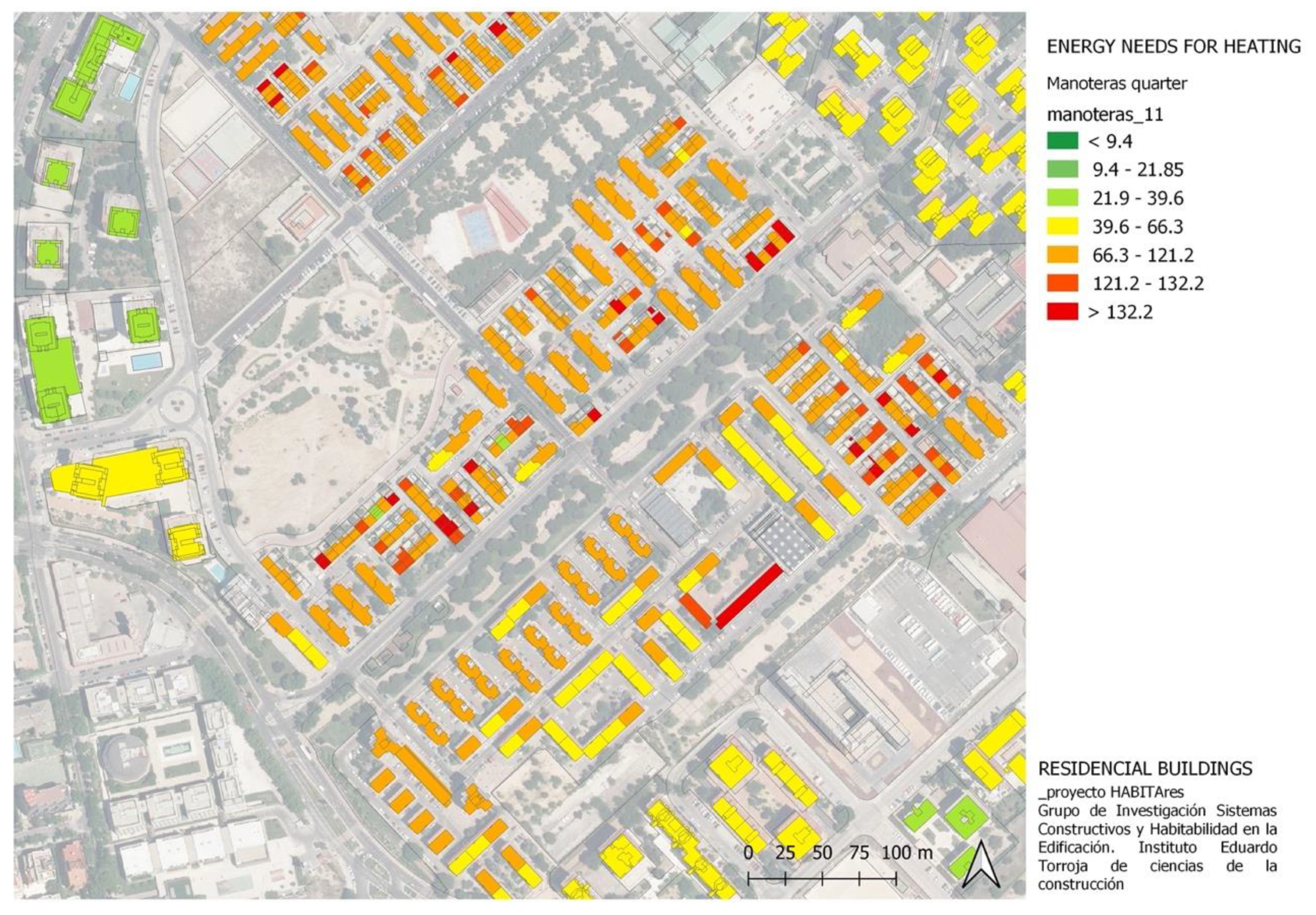
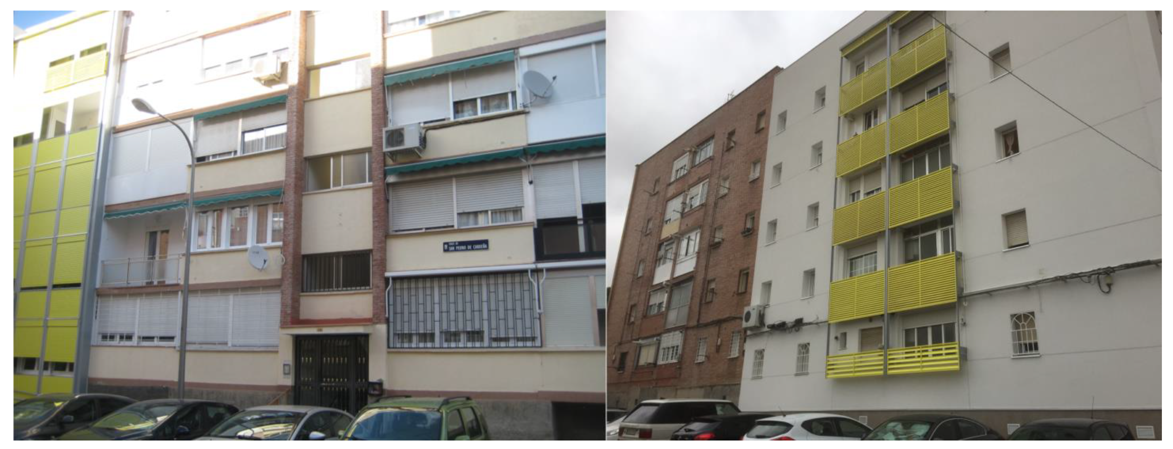
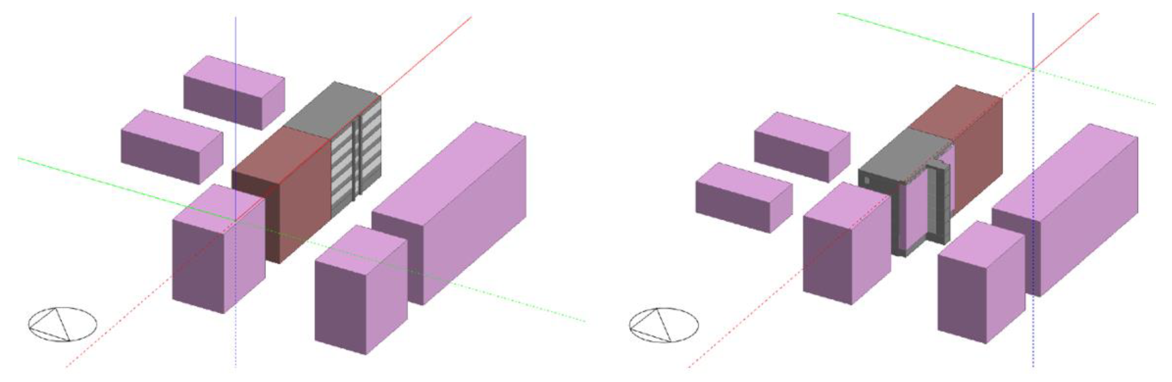
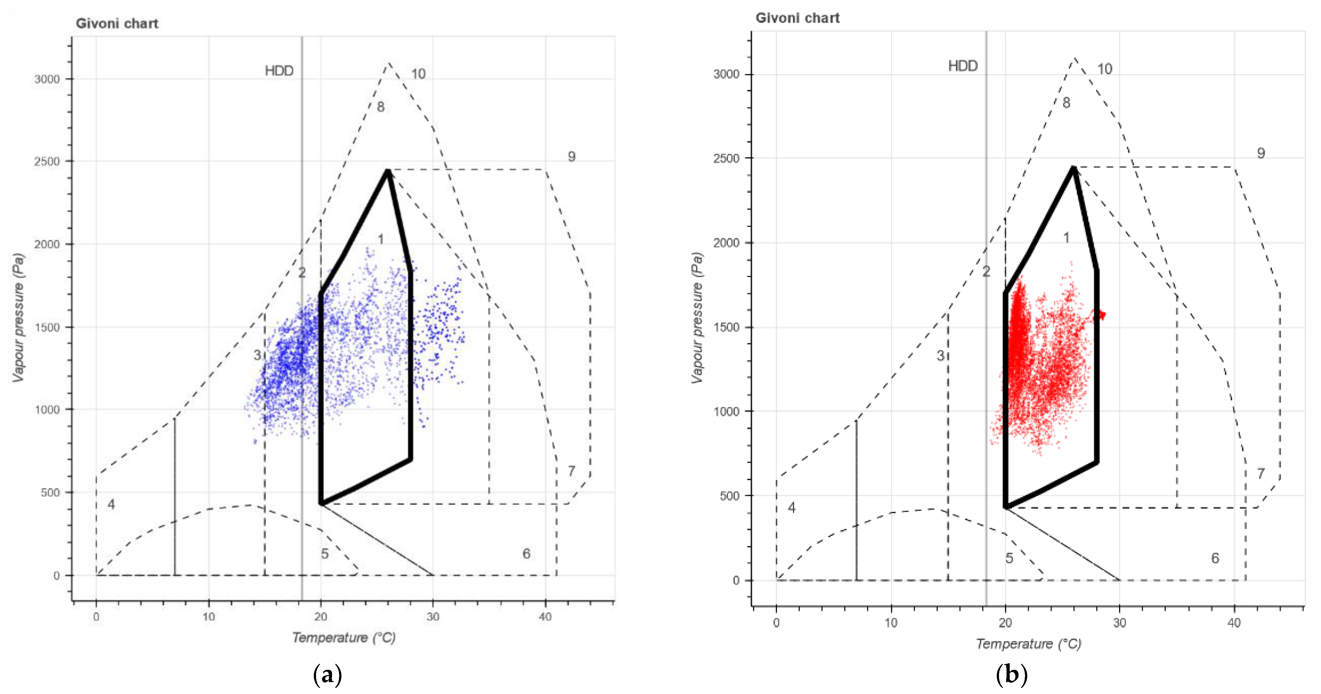
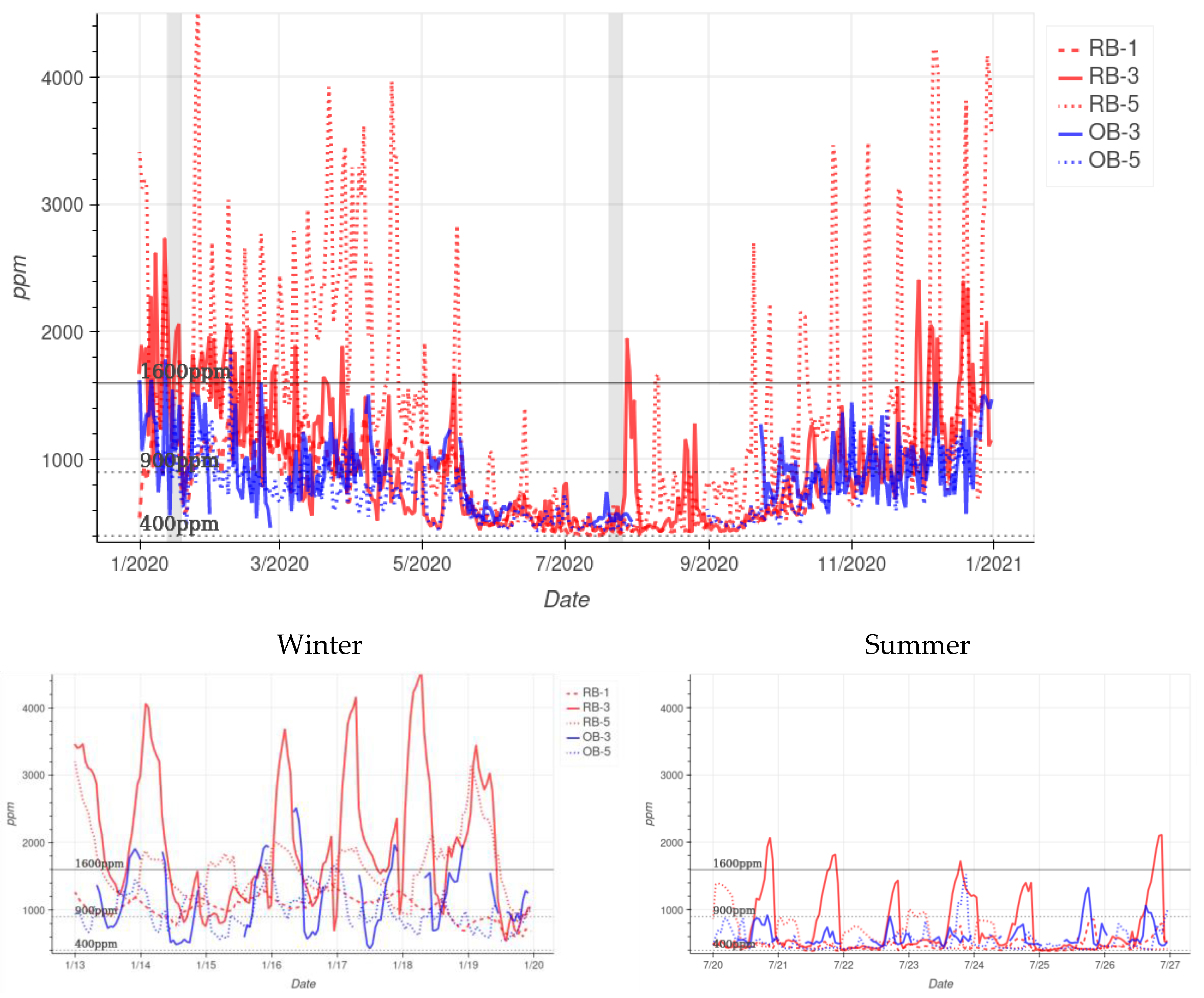
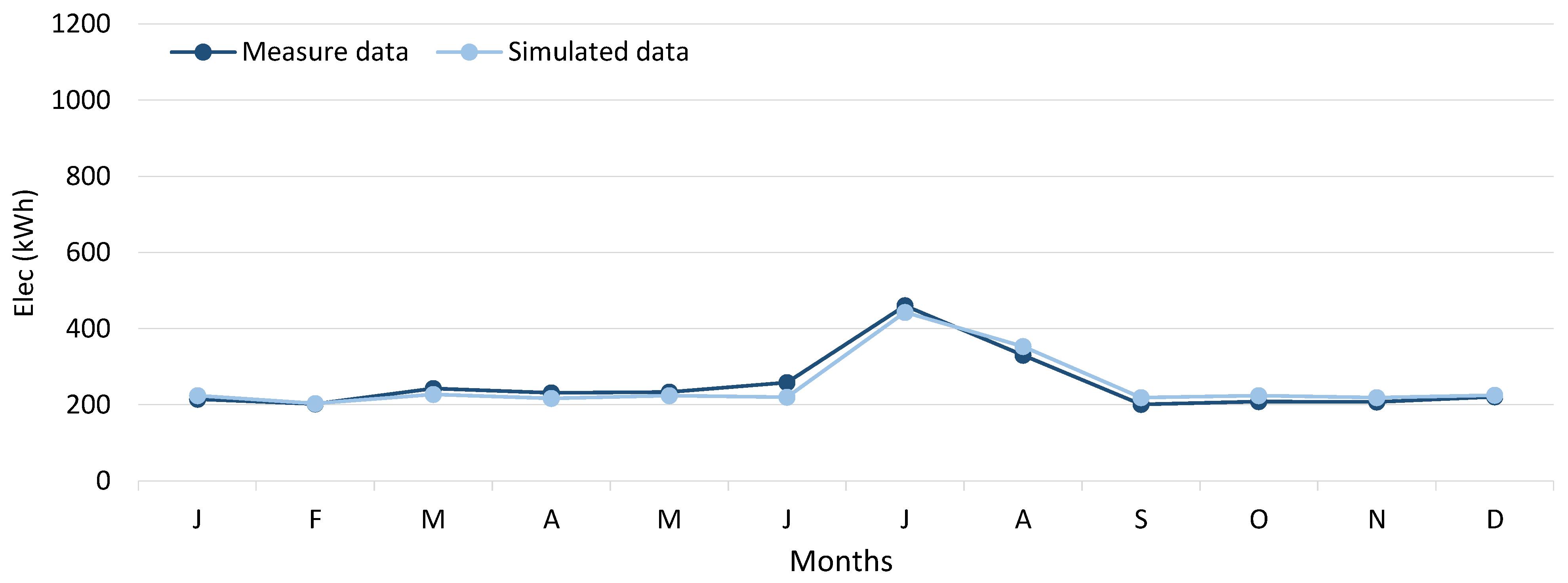


