
A Prior Semantic Network for Large-Scale Landcover Change of Landsat Imagery

1
Key Laboratory of Digital Earth Science, Aerospace Information Research Institute, Chinese Academy of Sciences, Beijing 100094, China
2
Airborne Remote Sensing Center, Aerospace Information Research Institute, Chinese Academy of Sciences, Beijing 100094, China
3
University of Chinese Academy of Sciences, Beijing 100049, China
*
Author to whom correspondence should be addressed.
Sustainability 2022, 14(20), 13167; https://doi.org/10.3390/su142013167
Submission received: 12 September 2022
/
Revised: 8 October 2022
/
Accepted: 10 October 2022
/
Published: 13 October 2022
(This article belongs to the Special Issue Regional Climate Change and Application of Remote Sensing)
Abstract
:Landcover change can reflect changes in the natural environment and the impact of human activities. Remotely sensed big data with large-scale and multi-temporal key characteristics provide the data support for landcover change information extraction. The development of deep learning provides technical method support for information extraction from remotely sensed big data. However, the current mainstream deep learning change detection methods only establish the changing relationship between two phases of images. They cannot directly extract the ground object categories before and after the change. It is easily affected by pseudo-changes caused by the color difference of multi-temporal images, resulting in many false detections. In this paper, we propose a prior semantic network and a difference enhancement block module to establish prior guidance and constraints on changing features to solve the pseudo-change problem. We propose a semantic-change integrated single-task network, which can simultaneously extract multi-temporal landcover classification and landcover change. On the self-made, large-scale multi-temporal Landsat dataset, we have performed multi-temporal landcover change information extraction, reaching an overall accuracy of 83.1% and achieving state-of-the-art performance. Finally, we thoroughly analyzed the landcover change results in the study area from 2005 to 2020.
1. Introduction
Landcover classification from remote sensing images is a significant application in remote sensing [1]. The classification of and changes in landcover can be obtained by using multi-temporal images. Landcover change can intuitively show the dynamic changes of the land surface, which has significant application value in land resource monitoring, ecological protection, urban expansion, returning farmland to forest, etc. [2,3,4,5,6]. However, the multi-temporal landcover classification also has more requirements on the amount of remote sensing data. With the development of remote sensing technology, remote sensing data is developing towards remotely sensed big data [7,8]. Remotely sensed big data with 4V characteristics volume, variety, velocity, and veracity provide massive data for remote sensing information extraction [9,10]. Traditional information extraction methods need to artificially design feature extractors according to data characteristics, such as index-based methods (NDVI, NDWI, NDBI, etc.) [11,12,13], texture-based methods (edge detection, keypoint extraction, etc.) [14,15,16], or statistical-based methods (support vector machines, random forests, etc.) [17,18,19]. When these methods face massive data, due to the limitations of artificial design, it is not easy to design a model that perfectly fits all the data. Therefore, the generalization ability of the model is limited, and the model may not be able to fit the new data. The emergence of deep learning technology has solved the data explosion problem of remotely sensed big data. Deep learning allows the network to independently exploit and learn effective features through deep convolutional neural networks (DCNNs) [20]. The DCNN has a stronger fitting ability to massive data and better generalization ability. At the same time, the deep learning method can quickly and accurately produce large-scale products, significantly saving time, human resources, and financial resources. Therefore, the deep learning method has gradually become the mainstream remote sensing information extraction method [21].
The traditional methods of landcover change detection are mainly based on two ideas [22,23,24,25,26]. The first is to set a change threshold based on the difference between the two images to detect the changing area. This method is largely limited by the quality of image processing. Differences in the colors of the two images are caused by differences in the imaging season and atmospheric conditions. As a result, pseudo-changes may appear in areas that have not changed between the two images. The second is to first classify the landcover of the two phases of images, then make the difference between the two phases of classification results to obtain the changed areas. This method is subject to the landcover classification accuracy for each phase of images. It may also be affected by the color difference between the images of the two phases. There may be errors in the classification results of the two phases, which will also cause pseudo-changes. These pseudo-changes and errors will cause changes in the ground objects to be inconsistent with the real natural scenes. The change detection methods based on deep learning establish a complex correlation between the two images by building a complex DCNN. The network learns the changing area’s features through supervised learning, eliminates the pseudo-changing area’s interference, and finally obtains a more accurate landcover change result.
Change detection methods based on deep learning have made significant development [27]. FC-EF [28] stacks two-phase images into multi-channel images, inputs images into a fully convolutional neural network, and outputs the changed regions. FC-Siam-conc [28] uses two encoders to extract the features of the two-phase images, respectively. It stacks each stage’s features, transfers them to the decoder for feature fusion, and outputs the changed regions. FC-Siam-diff [28] is similar to FC-Siam-conc. The only difference is that the two encoder feature fusion methods are replaced from stacking to difference operation. Similar to FC-EF, CDNet [29] stacks two-phase images into multi-channel images as input. It is a classic encoder–decoder architecture. Based on the dual encoder network, DSIFN [30] adds channel attention and spatial attention mechanisms to improve the detection accuracy of changing regions. UNet++MSOF [31] and DDCNN [32] stack two-phase images as input. The backbone of them adopts the densely connected UNet++ [33] network. These change detection methods can only find the changing area, which can be regarded as a changed/unchanged binary classification problem. For multi-class landcover change detection, the above methods cannot exploit semantic information in the changing area and often need to use additional semantic segmentation networks to supplement the semantic categories. Semantic segmentation in deep learning is pixel-level classification in remote sensing. Since the change detection of landcover requires pixel-by-pixel labels of multi-temporal registered images, there are few practical applications of large-scale landcover change detection based on deep learning methods. However, many studies still indirectly implement the change trend analysis after landcover classification of the multi-temporal images [34]. This paper is completely based on the deep learning method to detect the landcover changes of the multi-temporal images. The category information before and after the change in the ground objects can also be accurately classified.
We call change detection with semantic information before and after the change as semantic change detection. Landcover change is a semantic change detection task. In this paper, we propose a prior semantic network that integrates the difference enhancement block module and compresses the multi-task network into the single-task network, which implements high-precision Landcover change mapping and change details analysis.
In summary, the main contributions of this paper are as follows:
- We propose a prior semantic network architecture. Based on the two-phase data, the third-phase data and labels are introduced as prior constraint knowledge. It can solve the problem of pseudo changes caused by differences in color distribution and greatly improve the stability and robustness of change detection and semantic classification.
- We propose a difference enhancement block module, which weights the differences between the two branches, enhances true changes with large differences, and suppresses pseudo-changes with small differences.
- We compress the multi-task network, which is relatively independent of change detection and semantic segmentation, into a single-task network, which can simultaneously obtain the area of landcover change and the category of ground objects before and after the change in the network output.
- Extensive experiments on our self-made, large-scale, multi-temporal Landsat dataset achieve state-of-the-art performance. Through our proposed network, multi-temporal landcover change detection and specific change trend analysis were carried out for the large-scale study area from 2005 to 2020.
2. Methodology
This chapter mainly introduces the prior semantic network, the difference enhancement block module, and the single-task semantic change integration. We take the two-encoder Siamese UNet as the benchmark network. First, based on Siamese UNet, we add an additional encoder branch as a prior semantic knowledge constraint to build a prior semantic network. Then, the change feature fusion module in the prior semantic network is replaced with a difference enhancement block module to build PSNet-DBB. Finally, we combine the semantic segmentation and change detection multi-task decoders in PSNet into a single-task decoder to build PSNet-ST.
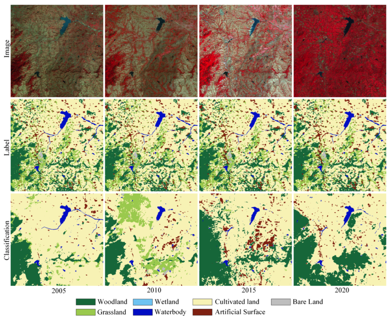
As shown in Figure 1, although the deep learning method can overcome the pseudo-change problem caused by color difference to a certain extent, the semantic information extraction is still unstable. The changing amplitude jitters seriously, and the change in the ground object category does not conform to the actual situation. The pseudo-changes may make it impossible to correctly obtain the change trend of the landcover and lose the practical application value. The current deep learning change detection network only extracts relevant information from the two-phase images, which is greatly affected by the color distribution of the images themselves. Based on the two-phase images, we can introduce another phase of images. The classification labels corresponding to the images of the new phase are also input into the network as auxiliary reference data for semantic information. It can improve the stability of the original two-phase image semantic information extraction, thereby improving the accuracy of landcover changes and ensuring the accuracy of changing trends. Therefore, we propose a prior semantic network architecture to achieve change detection under the constraints of additional reference branches.
Currently, in the mainstream change detection network using dual encoders, the feature fusion of the two branches is mainly performed through concatenation and difference operations. The concatenation operation simply stacks the features without enhancing the changing features. The difference operation expresses the feature difference of the two branches, but it causes the decoder to only have the change features and lose the semantic features. Therefore, we propose a difference enhancement block module, which enhances the features after the feature map difference is weighted to the original feature map as a weight. The module can amplify the obvious change features and suppress the features with very small differences. The reason for this is that such small changes are likely pseudo-changes caused by color differences. The module can also keep the original semantic classification information.
2.1. Prior Semantic Network
UNet is currently the most widely used fully convolutional neural network [35] and is often used as a baseline network in semantic segmentation and change detection. UNet is an encoder–decoder network with simple architecture, fast running speed, and low GPU memory overhead. We also choose UNet as the quasi-baseline network and ResNet-50 as the encoder. However, UNet has only one encoder branch. Two images must be stacked at the input end if the network is used for change detection. The network principle is similar to FC-EF. Therefore, we first add an encoder branch based on UNet, which is also ResNet-50 [36]. The weights of the two encoders are shared to build a Siamese UNet, named SiamUNet. Encoder weight sharing ensures that the feature positions in the two encoder branches are the same so that they are comparable to compute feature differences. The two branches of SiamUNet are fused by a concatenation operation to learn differential features. The network principle is similar to FC-Siam-conc. SiamUNet is the baseline network in this work, and the modules and structures proposed in this paper are gradually added based on the baseline network.
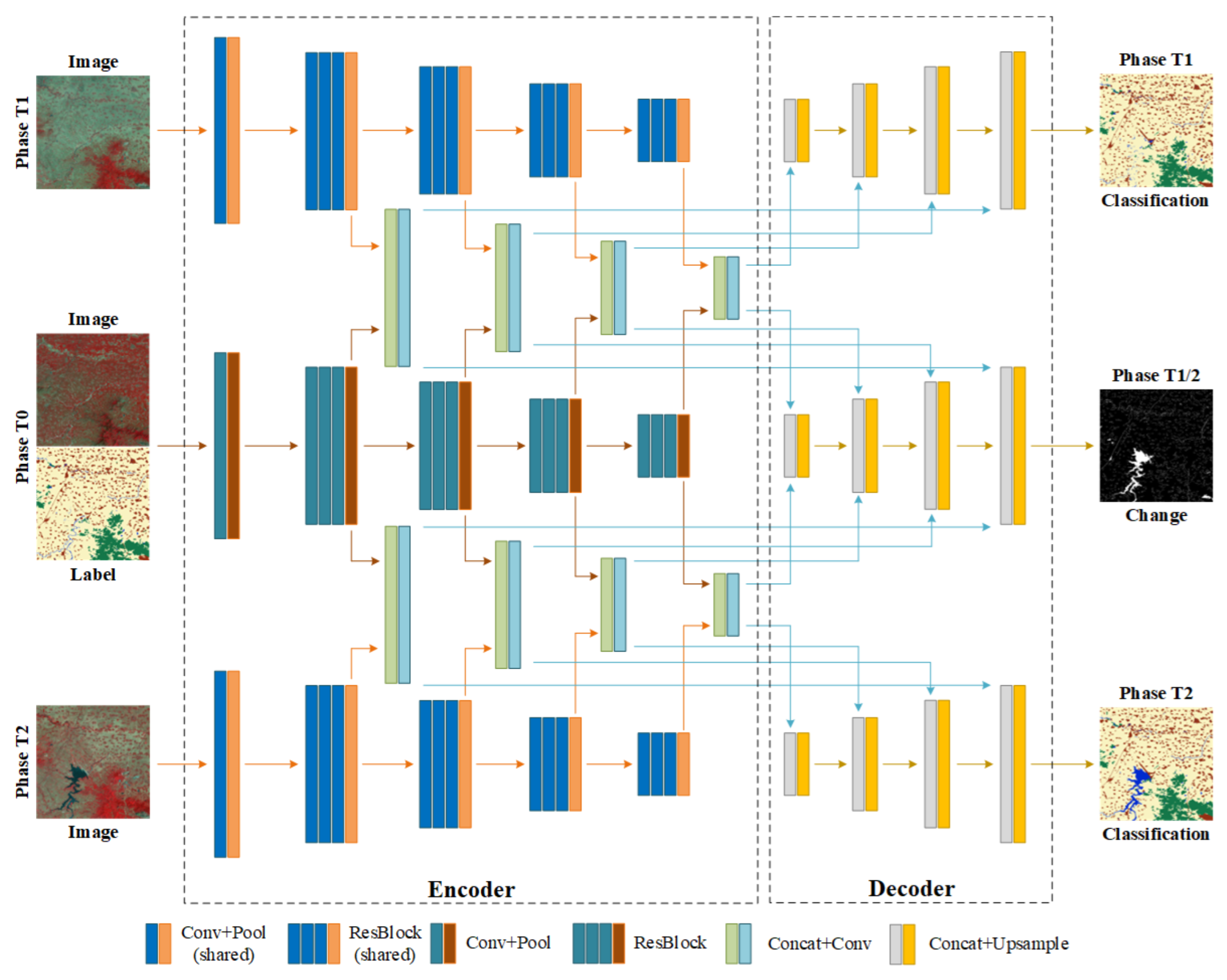
The two encoders of the dual-branch SiamUNet input image data of the T1 and T2 phases, respectively, and then detect the changing area between the T1 and T2 phases. We introduce an additional time-phase T0 of image and label data as prior semantic information, which is input into the network. Since the T0 phase requires label data as the additional input, the number of input channels is one more than that of the T1 and T2 phases. We add a new encoder branch, also ResNet-50, to extract T0 phase features. This branch does not share weights with the T1 and T2 phase branches. We named this branch the prior branch and named the T1 and T2 phase branches as the pre-change branch and post-change branch, respectively.
Unlike the direct fusion of the pre-change branch and post-change branch in SiamUNet, we first directly fuse the prior branch with the pre-change branch. The network builds a complex function map between T0 and T1 images by stacking many convolution operations and eliminates the effects of color differences by itself. The network will pay attention to the change feature information between the T0 and T1 images. With the help of the prior semantic information in the T0 label, the network will automatically establish more accurate semantic information for the T1 phase. The network will learn the differential features before and after the change in ground objects. This differential feature can be regarded as a change mapping feature. The network deduces the ground object category at T1 through T0 prior knowledge and change mapping features in changing areas. It will directly bring the prior semantics of T0 into T1 if there is no change between before and after. We obtain T1 features with T0 prior knowledge, named prior pre-change features. In the same way, we also fuse the prior branch with the post-change branch and establish the change feature association between T0 and T2 and the semantic information of the T2 phase. We obtain the T2 feature with T0 prior knowledge, named prior post-change feature.
Unlike SiamUNet, which can only learn T1 and T2 change features, prior pre-change and prior post-change features can learn the change features and use semantic information to assist in optimizing the change features. It is because the two change features contain the category semantic information of the ground objects, which can eliminate the interference caused by the pseudo-change phenomenon caused by the color difference in the image. In the decoder stage, the prior pre-change and prior post-change features are fused to calculate the changing area. This part of the decoder is called the change task decoder. In addition, the prior pre-change and prior post-change features independently calculate the semantic segmentation results. These two decoders are called segmentation task decoders. The entire network architecture is named the prior semantic network (PSNet), which can implement change detection and semantic segmentation at the same time. It is a multi-task network. The schematic diagram of the network architecture of PSNet is shown in Figure 2.
In the training stage, the images and labels of the T0 phase are stacked into the band data and input to the prior branch. T1-phase images are input to the pre-change branch as N-band data. T2-phase images are input to the post-change branch as N-band data. The pre-change branch shares weights with the post-change branch. The binary change label is used for the loss calculation at the end of the decoder of the change task, and the landcover classification labels of the T1 and T2 phases are respectively used for the loss calculation at the end of the decoder of the two shared weight segmentation tasks. All three loss values guide the backpropagation and gradient update of the network. In the inference stage, we only need to input the images and labels of the T0 phase and the images of the T1 and T2 phases. The changing area of T1 and T2 can be calculated, as well as the respective landcover classification results of T1 and T2.
2.2. Difference Enhancement Block Module
When calculating the changing area for the feature fusion of prior pre-change and prior post-change, if the common difference absolute value method is used to calculate the feature difference, a slight difference in the feature will be regarded as a change. This results in errors and pseudo-changes in the results. Because the features only contain differences, the decoder can only implement the change detection task. At this time, only a multi-decoder multi-task network architecture can be used for the semantic change detection task.
Therefore, we use the concatenation method to fuse the two features containing semantic segmentation information and keep all the feature information completely. At the same time, the square of the difference between the two features is calculated as the weight feature. Then, the fused features containing semantic segmentation information are weighted by the weight feature, which amplifies the changed features and suppresses the pseudo-changed features with minor changes. After the feature difference is squared, when the value is greater than 1, the feature difference weight will be amplified. When the value is less than 1, the feature difference weight will be reduced.
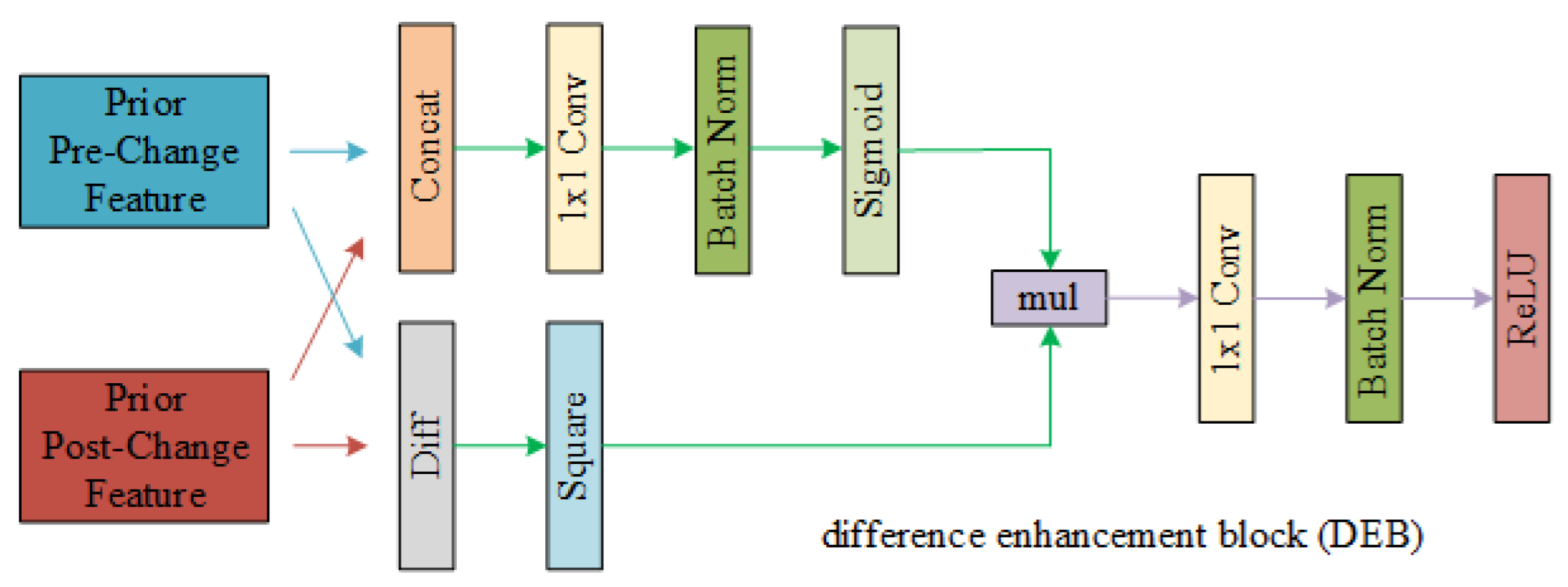
As shown in Figure 3, we first concatenate the prior pre-change and prior post-change features to obtain the fused features. Then we used convolution to reduce the number of channels of the fused features by half, the same as the number of channels before fusion. Batch normalization [37] and sigmoid are used to normalize and activate features. Then we calculate the difference square of the prior pre-change and prior post-change features to obtain the difference weight feature. Next, the difference weight feature is weighted to the fusion feature to obtain the difference-enhanced fused feature. Finally, convolution, batch normalization, and rectified linear unit (ReLU) are used to reintegrate, normalize, and activate the fused features to obtain the final difference-enhanced feature. We name it the difference enhancement block (DEB) module.
We denote the convolution operation as:
where ⊙ represents the convolution operator, represents the convolutional kernel, represents the vector of bias, and x represents the input data.
This section will perform the batch normalization operation after each convolution operation. To simplify the expression, not only represents the convolution layer but also includes the batch normalization layer. Therefore, the DEB module can be expressed as:
where ⊕ represents the concatenation operator; ⊗ represents the dot multiply operator; represents the sigmoid function; represents the ReLU function; and represents the first and second convolution layer, respectively; represents the prior pre-change feature; and represents the prior post-change feature.
We use the DEB module to replace the prior pre-change and prior post-change feature fusion modules in PSNet to build the PSNet-DEB network.
2.3. Single-Task Architecture for Semantic Change
There is certain independence between multiple decoders, which will prevent the features between multi-branches in the decoding stage from directly assisting and optimizing each other in the learning process. As a result, there will be minor contradictions between the semantic segmentation results and the change detection results. For example, the semantic segmentation results of the two phases have not changed, but the change detection results are considered to have changed. The single integrated decoder simultaneously implements semantic segmentation and change detection at the end of the network, which can optimize learning from each other and avoid conflicting problems.
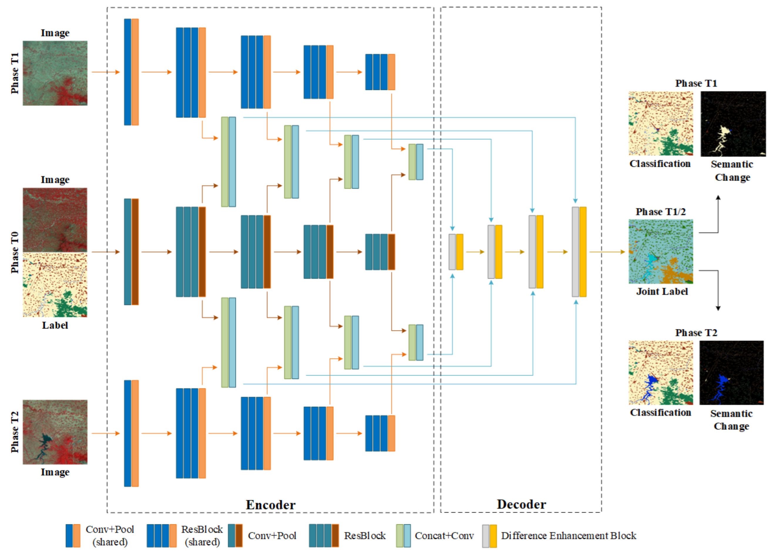
The DEB module in Section 2.2 can highlight the change feature information while keeping the complete semantic segmentation information, which provides a theoretical basis for building a single decoder to directly implement the semantic change task. We remove the two segmentation-task decoders in PSNet-DEB and keep only one change-task decoder. However, we change the output of the change-task decoder from binary-value change to the form of multi-value classification. We choose a number to describe the changing state between every two categories. For example, we label the first class change to the third class as 13, the fourth class change to the second class as 42, and the fifth class remains unchanged as 55. We rename the upgraded decoder as the semantic change decoder and build the PSNet-ST network. The schematic diagram of the network architecture of PSNet-ST is shown in Figure 4.
In the training stage, the input data form of PSNet-ST is the same as the multi-task PSNet. We use the joint label, which can describe the semantic change information, to compute the loss value and guide the network’s backpropagation and gradient updates. In the inference stage, we only need to input the images and labels of the T0 phase and the images of the T1 and T2 phases. Then, we can calculate the categories of the ground object before and after the change from T1 to T2 and deduce the changing area.
3. Experimental Results
3.1. Datasets
We can easily download multi-temporal Landsat imagery, which can be used to study landcover classification and change. However, no public Landsat dataset currently contains both semantic segmentation and change detection labels. Therefore, to test our proposed method’s performance on semantic change detection through experiments, we made a multi-temporal semantic change detection Landsat dataset.
We selected part of central and southern China as the study area, covering an area of 360,000 , located between E∼ E and N∼ N. We downloaded images of five time phases in 2000, 2005, 2010, 2015, and 2020. Each phase needs 26 images to cover the whole research area. The data path is between 121∼126, and the data row is between 36∼40. Among them, the images of 2000, 2005, and 2010 use Landsat-5 data, equipped with a thematic mapper (TM) sensor, including seven bands. Except for the thermal infrared band with a spatial resolution of 120 m, the other bands have a spatial resolution of 30 m. The images of 2015 and 2020 use Landsat-8 data, equipped with the operational land imager (OLI) sensor, including nine bands. Except for the panchromatic band, which has a spatial resolution of 15 m, the other bands have a spatial resolution of 30 m. All downloaded images are at the L1TP level. We only used six bands of data, including blue, green, red, near-infrared, shortwave infrared 1, and shortwave infrared 2. We then mosaicked the downloaded images by year and cropped them according to the latitude and longitude of the study area, removing redundant images outside the study area. Finally, we obtained 20,480 × 20,480 pixels of Landsat image in five phases. The spatial resolution is 30 m.
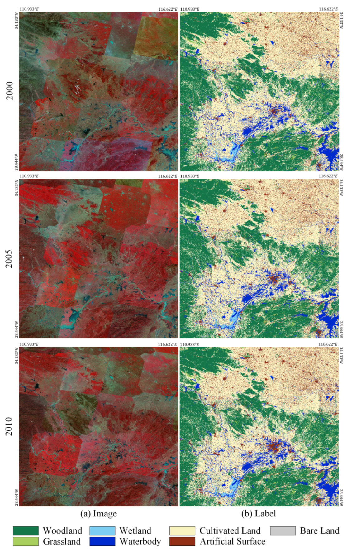
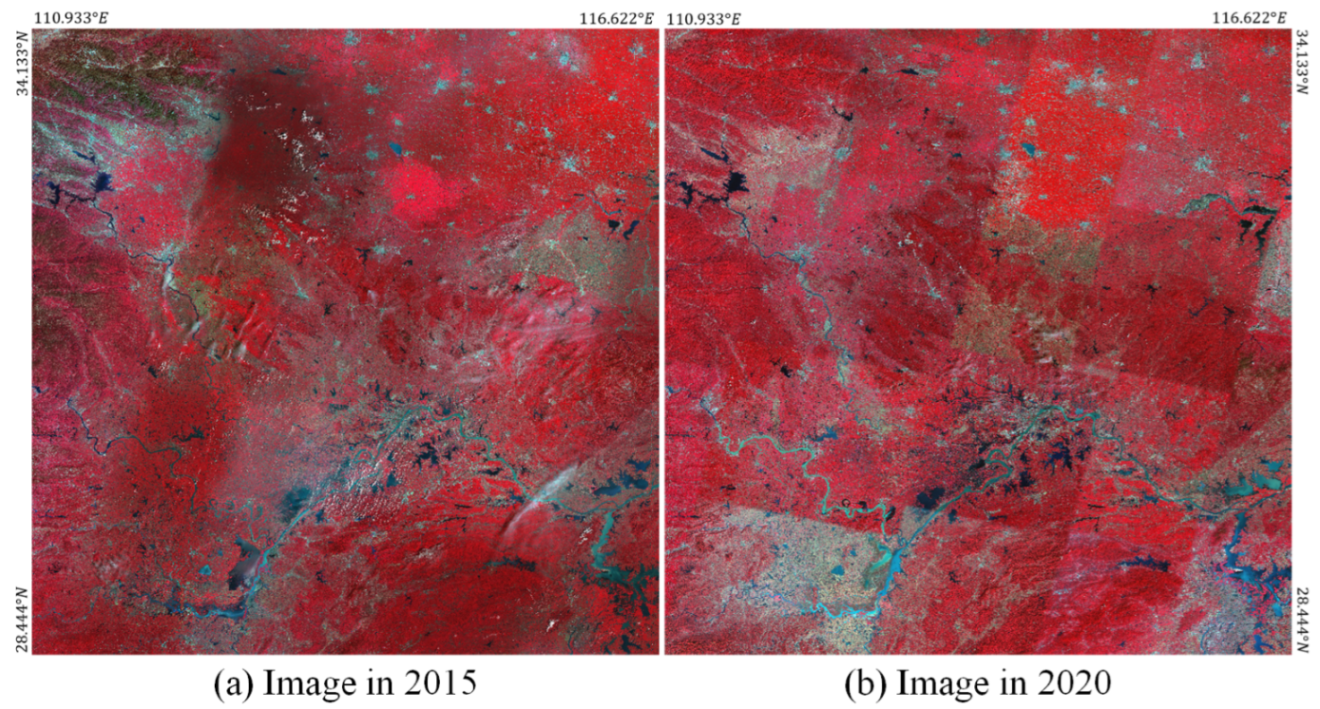
As shown in Figure 5, to train the semantic change model, we annotated the images from 2000, 2005, and 2010 at the pixel level, including seven categories: woodland, grassland, wetland, waterbody, cultivated land, artificial surface, and bare land. The 2015 and 2020 images shown in Figure 6 are not labeled, and the landcover classification and change results will be inferred through the deep learning method. All labels were visually interpreted in ArcGIS software by a team of 10. Controversial ground objects that cannot be identified on the image are labeled by high-resolution remote sensing images or field surveys. All samples were randomly cross-checked three times, and disputed samples were uniformly determined. Although there is a certain possibility of error in manual labeling, we try our best to minimize it and make the label’s accuracy as close to 100% as possible. High-resolution imagery is the primary reference for the edge of ground objects prone to mislabeling. Using the labels on the high-resolution images to downsample to the medium resolution can eliminate the label errors at the edge of the ground objects. To verify the model’s accuracy more accurately, we randomly selected 1000 points for each category of the ground object in the study area. Then, we obtained the ground truth corresponding to the 2020 images through a field survey and high-resolution image reference.
3.2. Implementation Details
3.2.1. Data Preprocessing
The PSNet network proposed in this paper requires two samples for change detection and one for prior knowledge input. Therefore, we take the sample in 2000 as prior knowledge and the samples in 2005 and 2010 as the data for actual semantic change detection. Since only two samples are needed for the published mainstream change detection network, we use samples in 2005 and 2010 for training to make the evaluation data the same.
We use the sliding window to crop each image with 20,480 × 20,480 pixels into 1600 small tiles with 512 × 512 pixels without overlapping. To evaluate the model’s generalization ability more objectively, we keep a large proportion of the data out of training. Therefore, we divide the dataset into a training set, validation set, and test set according to the ratio of 4:1:5. That is, 640 tiles are used for training the model, 160 tiles are used to validate intermediate model accuracy during the training stage to pick the best model, and 800 tiles do not participate in the training stage and are only used for prediction and accuracy evaluation.
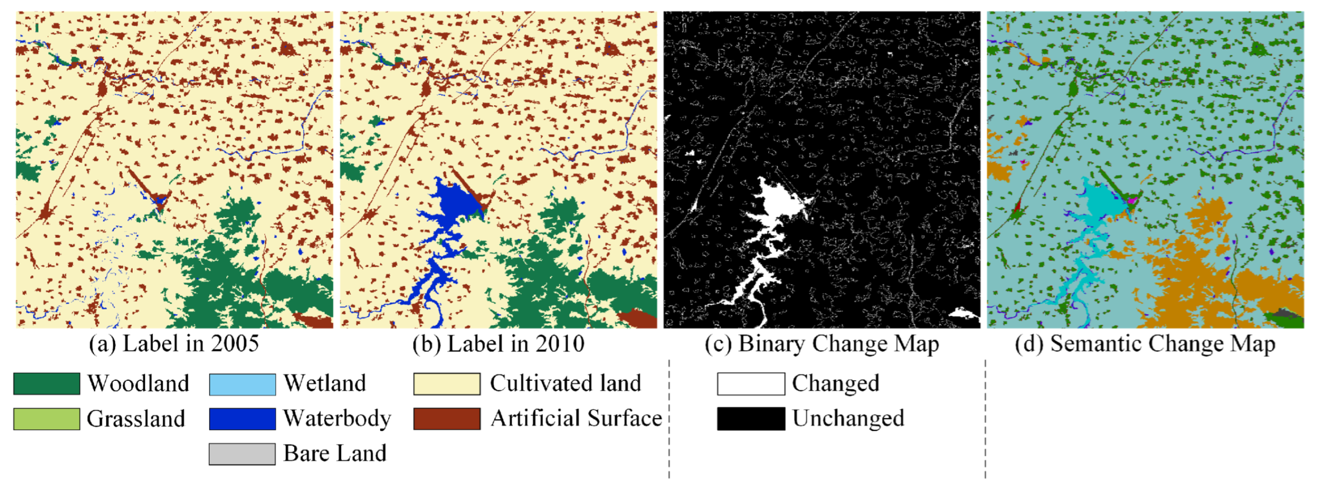
As shown in Figure 7, in addition to keeping semantic segmentation labels, the label data obtain binary change detection samples by comparing two-phase samples with different values. We adopt the form of joint labels to make semantic change labels. We use a two-digit number to denote each pixel’s categories before and after changes. The first digit is the category number before the change, and the second is the category number after the change. When the two digits are the same, there is no change. The category numbers in semantic change map are shown in Table 1. The columns indicate the categories before the change, and the rows indicate the categories after the change.
To ensure a more reasonable distribution of data input to the model, we normalize the input data first. The data normalization is defined as:
where represents the normalized image data, I represents the original input image data, represents the mean value of each band in the image data, and represents the standard deviation value of each band in the image data.
3.2.2. Training Settings
We use the PyTorch deep learning framework [38] to implement the PSNet proposed in this paper and other mainstream change detection networks published. We used four NVIDIA RTX 3090 GPUs with 24 GB memory to train the model. Data augmentation operations include random horizontal flips, random vertical flips, and random rotation. The optimizer is AdamW [39], and the batch size is set to 32. The initial learning rate is and gradually increases to during the first 10 epochs. Then, the learning rate is automatically adjusted using the model validation accuracy. When the accuracy has not improved for 20 consecutive epochs, the learning rate is multiplied by the drop coefficient of 0.3. When the learning rate drops to , the training process ends.
The formula of the early learning rate increasing stage is:
where represents the real-time learning rate, represents the initial learning rate, represents the maximum learning rate, t represents the real-time training iterations, k represents the number of iterations per epoch, and e represents the number of training epochs when the learning rate reaches the maximum value.
The formula of the later learning rate automatic decreasing stage is:
where represents the decreased learning rate, represents the learning rate before decreasing, and represents the drop coefficient.
The cross entropy loss can optimize the model by pixel level. Lovász-softmax [40] loss can optimize the model by region level and from intra-class and inter-class differences. Therefore, we choose cross-entropy loss and Lovász-softmax loss as loss functions to train the network. The binarized version corresponding to the two losses is selected in the binary change detection task. The task loss is calculated as follows:
3.2.3. Evaluation Metrics
We mainly adopt three evaluation metrics: overall accuracy (OA), intersection over union (IoU), and F1 score. OA represents the proportion of correctly classified pixels among all pixels. IoU is used to evaluate the accuracy of a certain class, where intersection refers to the number of correctly classified pixels, and union refers to the sum of the number of correctly classified and misclassified pixels. The F1 score is also used to evaluate the accuracy of a certain class, taking into account both precision and recall.
We denote all pixels according to the following rules: means the label is true and the prediction is true. means the label is false and the prediction is true. means the label is true and the prediction is false. means the label is false and the prediction is false.
The formula for OA is as follows:
The formula for IoU is as follows:
F1 score is calculated by and :
where and are calculated by , , and :
For multi-task PSNet, the binary change detection accuracy is evaluated with IoU and F1 scores. The semantic segmentation task evaluates single-class accuracy using the F1 score and overall accuracy using mean F1 score (mF1) and OA. Semantic change detection accuracy for single-task PSNet-ST using F1 score was used to evaluate the accuracy of each change.
3.3. Comparing Methods for Binary Change Detection
Since other published mainstream change detection networks can only implement binary change detection, to verify the effect of the prior semantic branch and DEB module proposed in this paper, we use the PSNet series for binary change detection tasks for a fair comparison. Table 2 shows the quantitative accuracy comparison of mainstream change detection networks and the PSNet series used in this paper. It can be seen that the F1 score of the mainstream change detection network can only reach 44.81%. The accuracy of most networks can exceed 30%, and the accuracy of FC-Siam-diff and DDCNN is lower. The baseline SiamUNet built based on the idea of UNet and Siamese encoder in this paper can reach 49.06%. A prior branch is added to the baseline, and the images and labels of the prior reference phase are used for additional constraints. The accuracy of the PSNet can reach 62.79%. It can be seen that prior knowledge is very effective in improving accuracy. Based on PSNet, we replace the multi-branch encoder feature fusion module with the DEB module proposed in this paper. The DEB module performs filtering, weighting, and optimizing the changing features. The PSNet-DEB network achieves 68.62% accuracy. Therefore, using feature differences to weight, optimize and fuse the features has a certain effect on improving accuracy. Finally, based on PSNet-DEB, the semantic segmentation and change detection decoder are combined to build PSNet-ST. The single-task decoder is used to directly learn the categories of ground objects before and after the change. Since the two tasks can be optimized for each other after the decoder is integrated, the accuracy of change detection is greatly improved, reaching 80.91%.
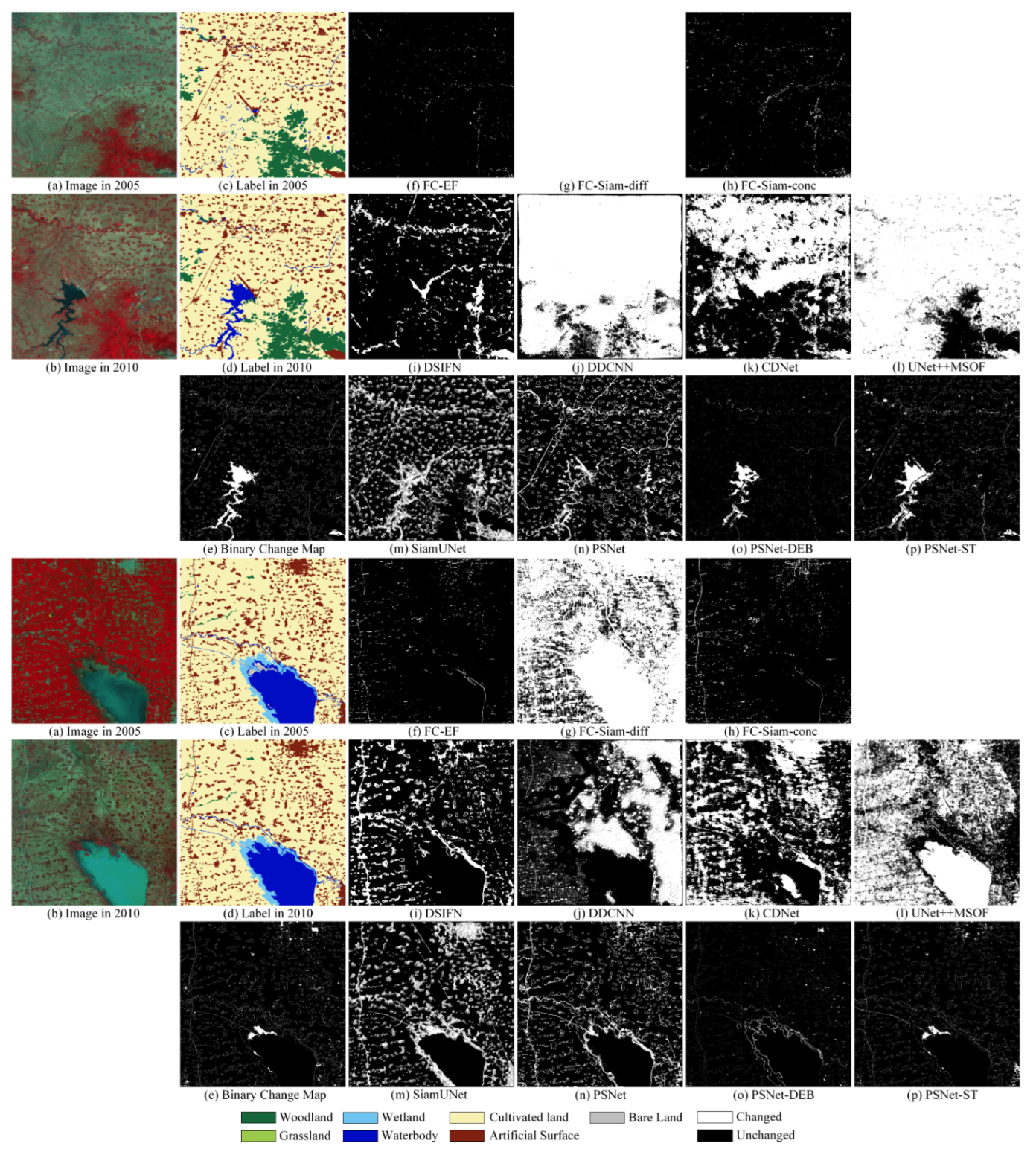
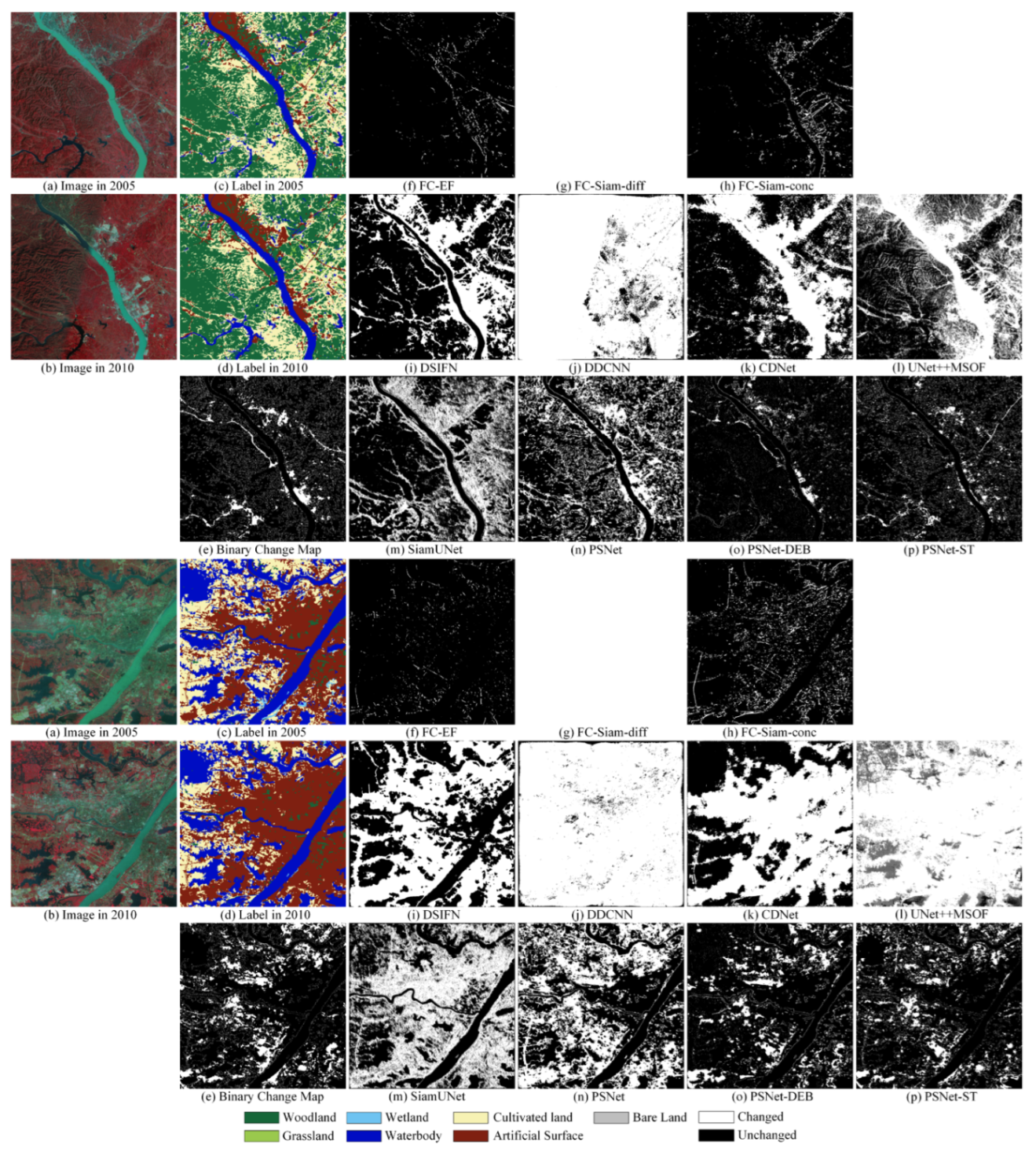
We visualize the change detection results of the mainstream change detection network and the PSNet series network proposed in this paper. Figure 8 shows comparison charts of the change detection results. In the first group, it can be seen that the errors of the three methods, FC-Siam-diff, DDCNN, and UNet++MSOF, are very obvious, and the change detection fails. The error of the CDNet result is also more conspicuous. FC-EF, FC-Siam-conc, and DSIFN missed changes in waterbodies. SiamUNet can detect changes in waterbodies, but there are many false detections. After adding prior knowledge constraints, PSNet can reduce some false detections. After using the DEB module, the waterbody changes detected by PSNet-DEB are more accurate. However, many small changes are missed since DEB modules inhibit small changes, and multi-task decoders cannot directly assist each other in the learning stage. For the single-task network PSNet-ST after multi-decoder integration, the change results of waterbody are very accurate, and other small changing objects can also be detected smoothly.
In the second group, the errors of FC-Siam-diff, UNet++MSOF, and DDCNN are very obvious. It can be seen from the images that there is no major change in the two phases of the ground objects. However, due to the impact of imaging conditions and seasonal factors, the cultivated land shows completely different colors in the images of the two phases. It also brings more significant challenges to change detection. Without the constraints of prior knowledge, baseline SiamUNet, like other mainstream networks, has many false detections. While the prior knowledge assists PSNet in reducing the false detection rate, the DEB module further eliminates small patches with false detections. After the PSNet-ST integrated decoders, the changes in the waterbody can be correctly detected, and the very small changes that have been eliminated in PSNet-DEB can also be successfully detected. More comparisons can be found in Appendix A.1.
To sum up, FC-Siam-diff and DDCNN almost completely fail for change detection on 30 m resolution Landsat images. FC-EF and FC-Siam-conc mainly show more missed detections, while DSIFN, CDNet, and UNet++MSOF show more false detections. In our proposed method, the effect of adding one phase image as prior knowledge is pronounced. Although some false detections exist, the detected change contours are gradually approaching the labels. The DEB module can suppress a large number of false detections. However, semantic segmentation and change detection tasks are independent of each other. The semantic segmentation results cannot be used to optimize the change detection results. Therefore, there will be over-suppression, and small change areas will be missed. After the semantic segmentation and change detection tasks are combined into a single task, the features are optimized for each other. The advantages of the prior semantic information and the DEB module are integrated, and the shortcomings are overcome. The best change detection performance is achieved.
3.4. Comparing Methods for Semantic Change Detection
Since other mainstream change detection networks cannot achieve change detection tasks with semantic information, we only compare the baseline SiamUNet, PSNet, PSNet-DEB, and PSNet-ST networks. SiamUNet has no prior knowledge constraints, and the two decoders for semantic segmentation and change detection tasks are independent and belong to a multi-task network. PSNet has prior knowledge constraints, the two decoders of semantic segmentation and change detection tasks are separated, and it is also a multi-task network. PSNet-DEB is basically the same as PSNet, except that the DEB module replaces the multi-branch feature fusion module, and the feature difference is used for feature weighting enhancement. PSNet-ST has prior knowledge constraints and the DEB module for feature optimization. The single decoder implements the simultaneous extraction of the ground object categories of the two phases. Therefore, semantic segmentation and change detection tasks can be performed simultaneously, which belongs to a single-task network.
Table 3 shows the quantitative accuracy comparison of landcover classification between SiamUNet and PSNet series networks. The OA of baseline SiamUNet is 83.45%, and the accuracy of grassland, artificial surface, and bare land is relatively low. After adding prior knowledge constraints, the OA of PSNet reaches 92.77%, and the accuracy of each category is significantly improved. After the DEB module is integrated with the multi-decoder, the accuracy is further improved. The OA of the final single-task network PSNet-ST can reach 94.26%. Table 4 shows the accuracy comparison of SiamUNet and PSNet series network with ground truth in 2020. All methods showed a downward trend in accuracy. Without prior knowledge constraints, SiamUNet has the most severe drop in accuracy. The PSNet series network has only a slight decrease in accuracy, which shows that with the prior knowledge constraints, the network’s generalization ability has been significantly improved. The OA of the best-performance network PSNet-ST can reach 92.99%, which means that out of 7000 ground truth points, 6509 points are correctly classified.
For the quantitative accuracy evaluation of semantic change detection, we construct a matrix indicating the mutual conversion to describe the change accuracy between any two categories. As shown in Table 5, the column represents the object category before the change, and the Mean Out column represents the mean F1 score calculated based on the category before the change. The row represents the object category after the change, and the Mean In row represents the mean F1 score calculated based on the category after the change. Diagonal elements indicate that the ground object has not changed. Table 5, shows the semantic change detection accuracy between any two categories in the results of SiamUNet, and the overall mean F1 score is 63.1%. Table 6 shows the semantic change detection accuracy between any two categories in the results of PSNet, and the overall mean F1 score is 73.25%. Table 7 shows the semantic change detection accuracy between any two categories in the results of PSNet-DEB, and the overall mean F1 score is 79.07%. Table 8 shows the semantic change detection accuracy between any two categories in the results of PSNet-ST, and the overall mean F1 score is 83.10%. It can be seen that prior constraint knowledge, DEB module, and single-task integration can significantly improve the semantic change detection task.
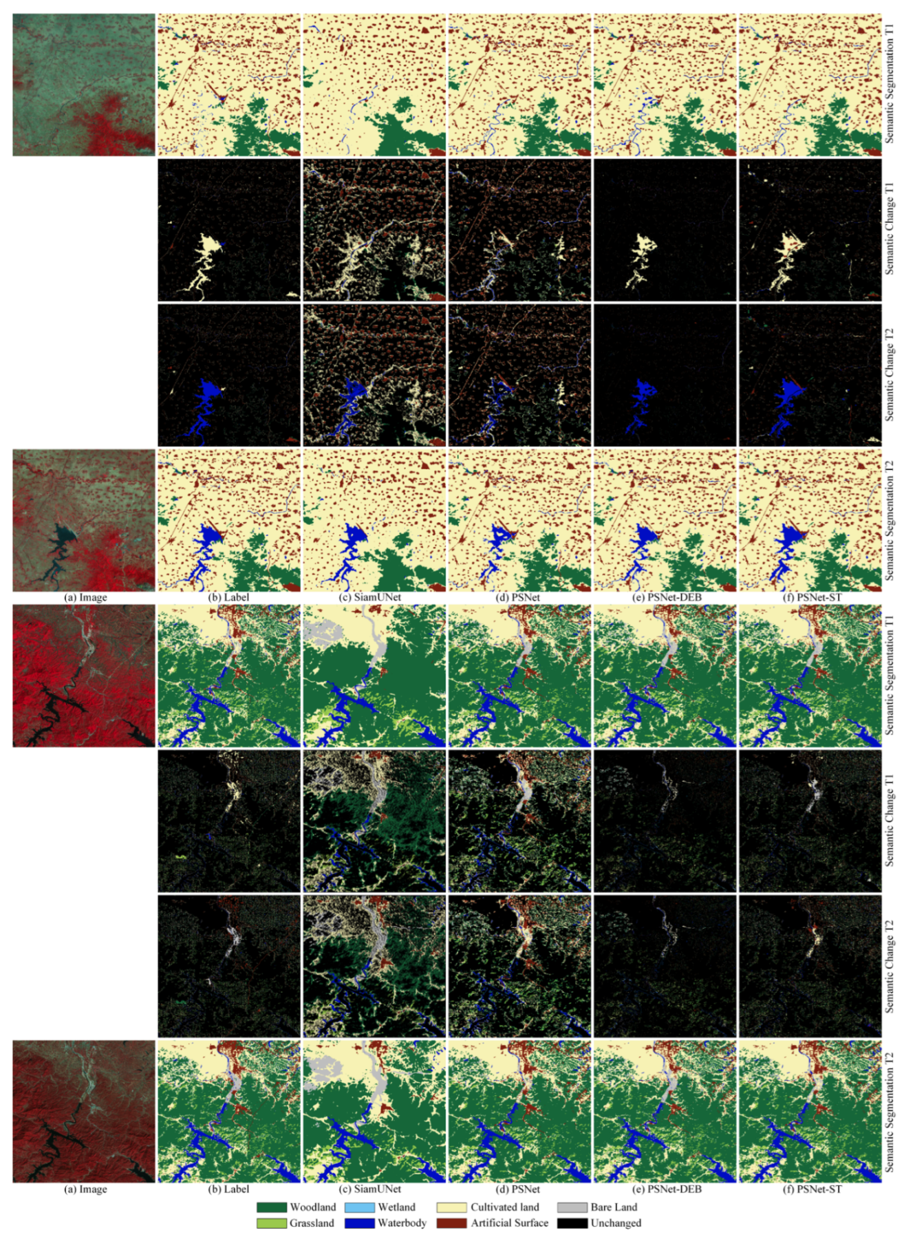
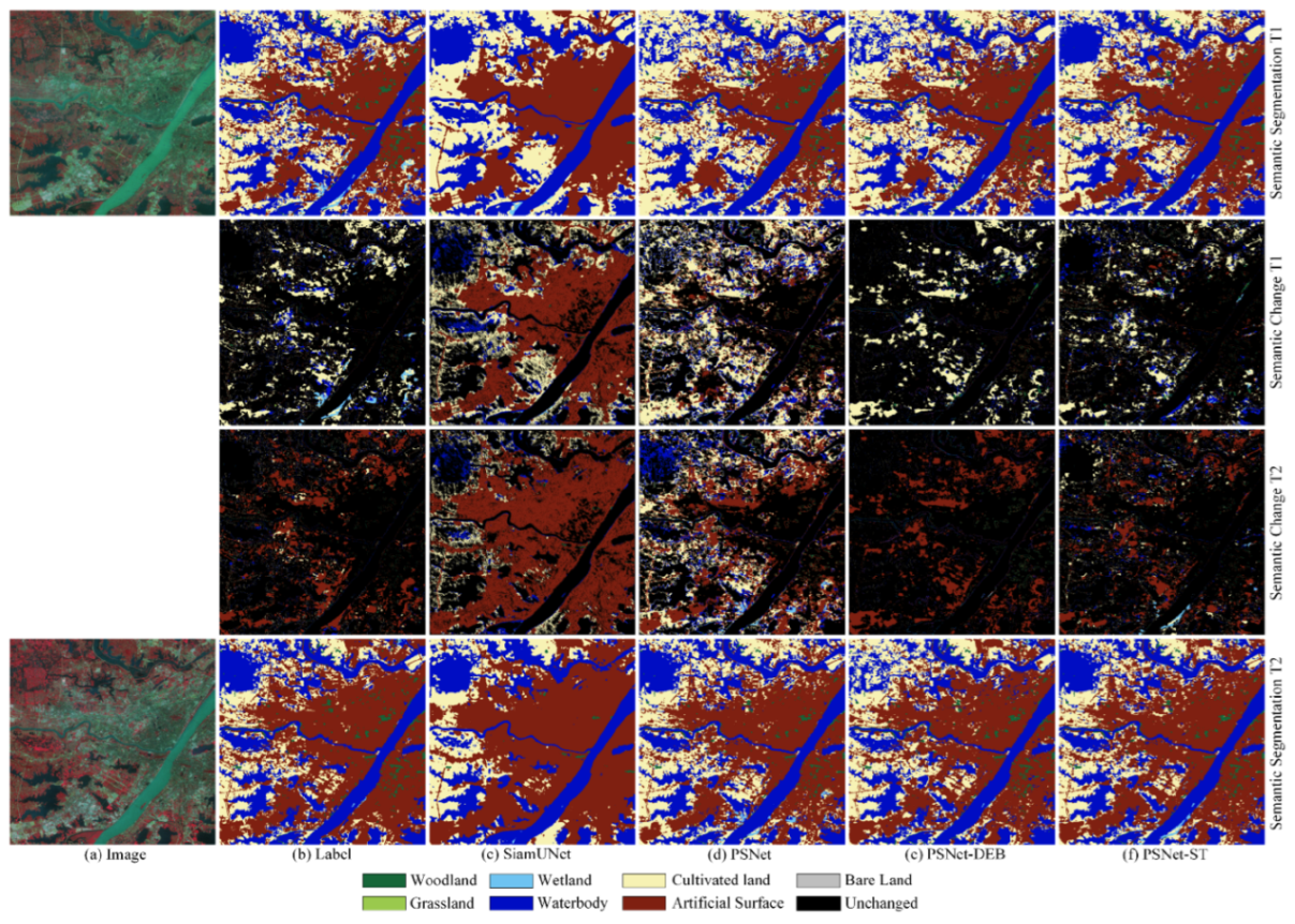
We visualize the semantic change detection results of baseline SiamUNet and the PSNet series networks proposed in this paper. Figure 9 is a comparison chart of the semantic change detection results. In each set of examples, the first line is the landcover classification results in the pre-change phase. The second line is the classification results before the change in the changing area. The third line is the classification results after the change in the changing area. The fourth line is the landcover classification results in the post-change phase.
In the first group, the main change is that the cultivated land becomes the waterbody, with some other minor changes. SiamUNet’s landcover classification results are not detailed enough, and small objects are missed. Due to false detections in the change detection, there are errors in the changing area that the before-and-after phases do not in fact change. PSNet has fewer false detections with the help of prior knowledge constraints. However, due to the impact of multi-task independent decoders, the change detection result contradicts the result of semantic segmentation. That is, the change detection branch believes there has been a change, and the semantic segmentation branch believes the ground objects in the before-and-after phases are the same. Smaller fragmented changes are missed from the PSNet-DEB results. PSNet-ST has excellent landcover classification results and change results. After integrating the multi-task decoder into a single-task decoder, the inconsistency between the two results has been eliminated.
In the second group, similar to the first group, the classification results of SiamUNet’s landcover are not detailed enough, the change detection error is obvious, and a large number of unchanged ground objects are placed in the changing area. With the help of prior knowledge constraints, PSNet has fewer false detections, and the changing area is still too large. The result of PSNet-DEB is close to the label, but the bare land’s change in the middle of the image is fragmented and missed. PSNet-ST completely extracts the undetected bare land in PSNet-DEB. It can all be extracted, whether it is a large or a small change. The landcover classification results of the two phases are also very accurate. More comparisons can be found in Appendix A.2.
In summary, the prior semantic knowledge constraints, DEB module, and single-task integrated decoder strategy proposed in this paper have achieved state-of-the-art performance in Landsat’s semantic change detection task.
4. Discussion
In this section, based on the best-performing PSNet-ST model in Section 3, we perform semantic change detection on the four-phase images of the study area in 2005, 2010, 2015, and 2020 and obtain large-scale landcover change results. In addition, the samples in 2000 are used as prior knowledge to assist and constrain the other two phases of data for training and prediction. In addition to this section, more details on these results can be found in Appendix B.
To count the process state of the mutual changes between the ground objects, we adopted a category transition matrix to represent the mutual change areas. As shown in Table 9, the column represents the area of a certain category becoming other categories. The Total Out column represents the total area of a certain category turning into other categories, which can be regarded as the transfer-out. The row represents the area of each other category turned into a certain category. The Total In row represents the total area of other categories turned into a certain category, which can be regarded as the transfer-in. The Total Change row represents the overall area change of each category, which is calculated by combining the transferred-out and transferred-in areas of the category.
4.1. Analysis of Landcover Change from 2005 to 2010
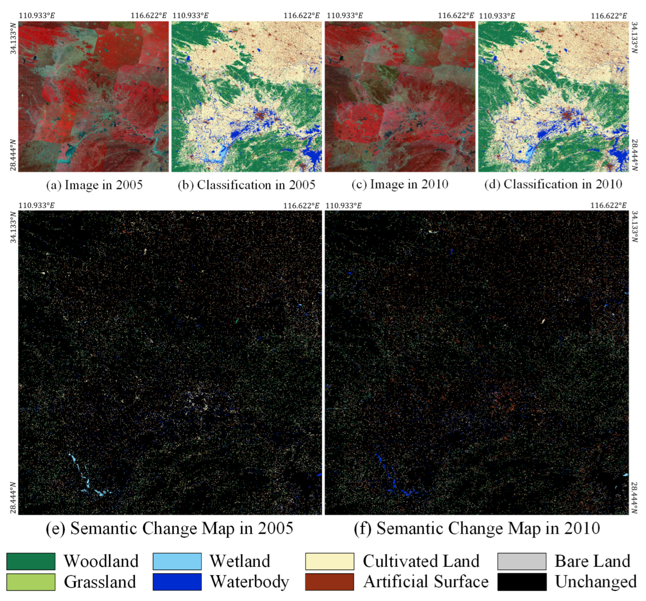
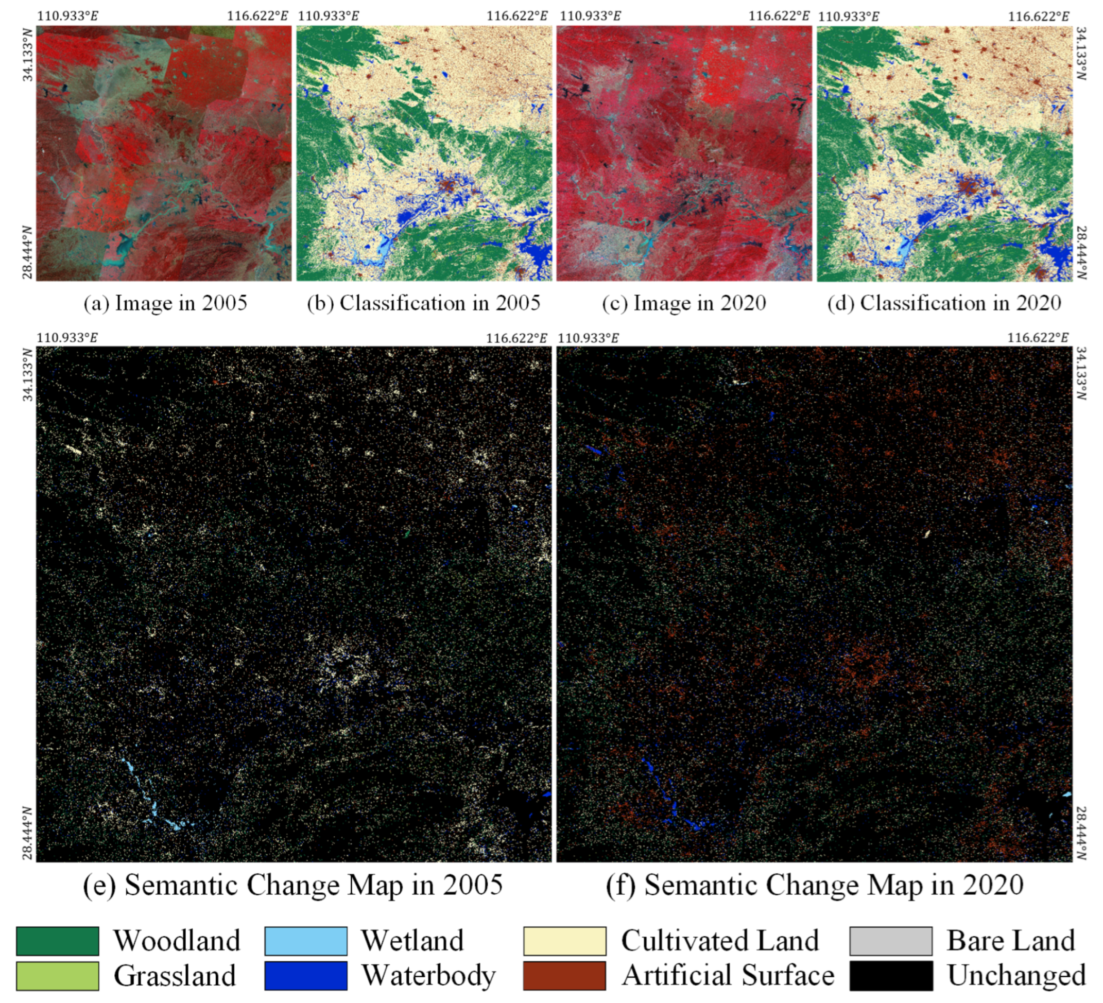
The landcover change in the whole study area from 2005 to 2010 is shown in Figure 10. The figure shows the landcover classification results in 2005, the landcover classification results in 2010, and the two-phase corresponding ground object classes in the changing area. Equivalent to the ground objects in Figure 10e becomes the ground objects in Figure 10f. Table 9 is the category transition matrix of the two-phase landcover changes. It can be seen that from 2005 to 2010 in the study area, the woodland, grassland, and bare land changed very little. The wetland area becomes smaller, and the water body area increases. The cultivated land area decreased more, while the artificial surface area increased more. A more specific analysis shows a mutual exchange between woodland and cultivated land. It is caused by the interaction between returning farmland to forest and cutting down trees for reclamation. As the main feature of greening, the woodland area remains unchanged. There is less exchange between grassland and cultivated land, as deserted arable land grows weeds, which can also be reclaimed for cultivation. There is a mutual exchange between wetlands and waterbodies. This is due to the similarities between wetlands and waterbodies. Shallow tidal flats submerged by water will be classified as wetlands. Affected by the imaging season, there will be a mutual conversion between wetlands and waterbodies. There is also a small exchange between waterbodies and cultivated land. This is because when there is more water storage in paddy fields, it looks similar to waterbodies. Since urban development is on a trend of continuous expansion, artificial surfaces occupy more cultivated land. The cultivated land around the city is changed to artificial surfaces. With urbanization, the rural population and the area of cultivated land decrease, and the migration of the rural population to cities will make urban expansion a usual trend. Some villages were demolished to build new reservoirs. However, some of the demolished village lands were planted with trees and converted into woodland. At the same time, some urban artificial surfaces have been re-planned as forest parks. Therefore, in five years, many artificial surfaces have been converted into waterbodies and woodland. More changes’ details can be found in Appendix B.1.
4.2. Analysis of Landcover Change from 2010 to 2015
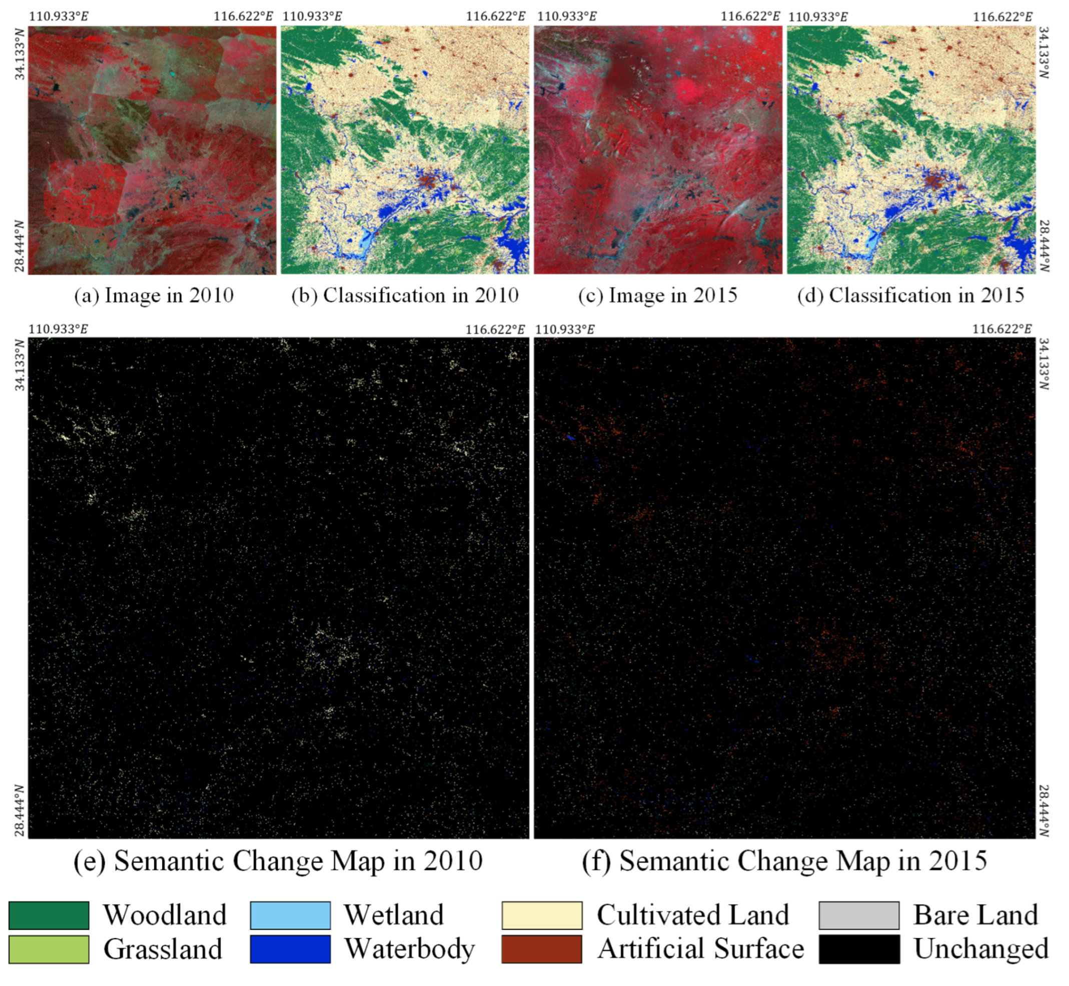
The landcover change in the whole study area from 2010 to 2015 is shown in Figure 11. The figure shows the landcover classification results in 2010, the landcover classification results in 2015, and the two-phase corresponding ground object classes in the changing area. The ground objects in Figure 11e become equivalent to the ground objects in Figure 11f. Table 10 is the category transition matrix of the two-phase landcover changes. It can be seen that from 2010 to 2015, the changes in grassland, wetland, and bare land were very small in the study area. The changes in woodlands and waterbodies are also not obvious enough. The area of cultivated land decreased more, while the artificial surface area increased more. A more specific analysis shows a mutual exchange between woodland and cultivated land. The mutual exchange between the waterbody and the cultivated land is also similar to the last five years because when there is more water in a paddy field, it looks similar to a waterbody. Cultivated land continues to be transformed into artificial surface, indicating that urbanization further devours the surrounding cultivated land. Compared with the last five-year changes, the area of cultivated land has decreased more, and the artificial surface area has also increased. This shows that the economy has developed faster in the past five years. The speed of urbanization has also accelerated. More details on these changes can be found in Appendix B.2.
4.3. Analysis of Landcover Change from 2015 to 2020
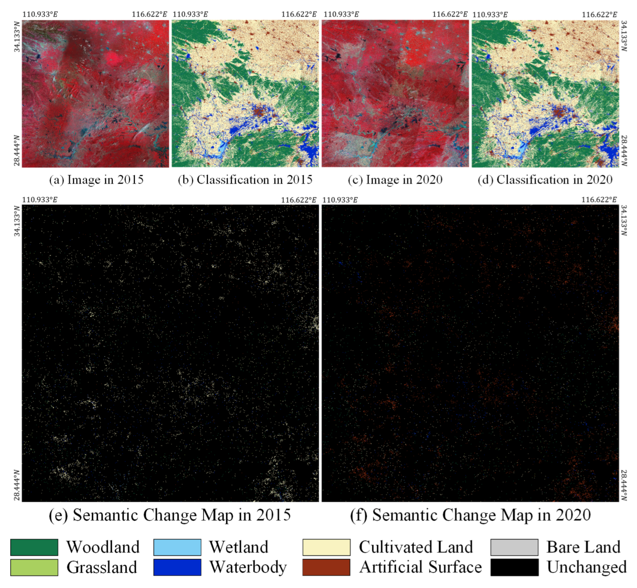
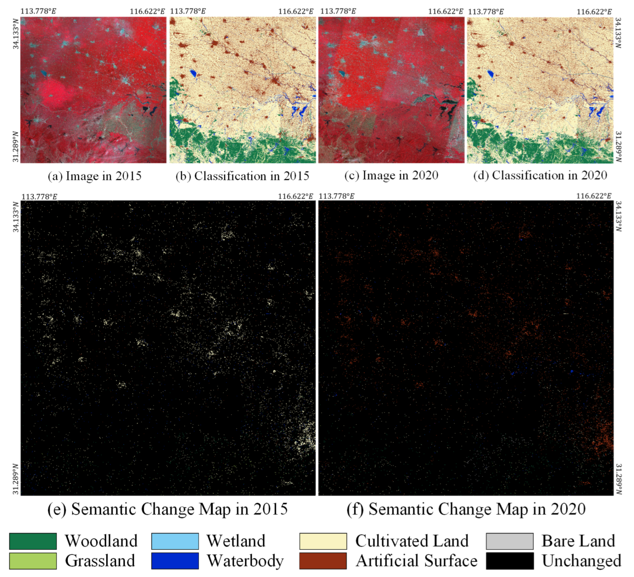
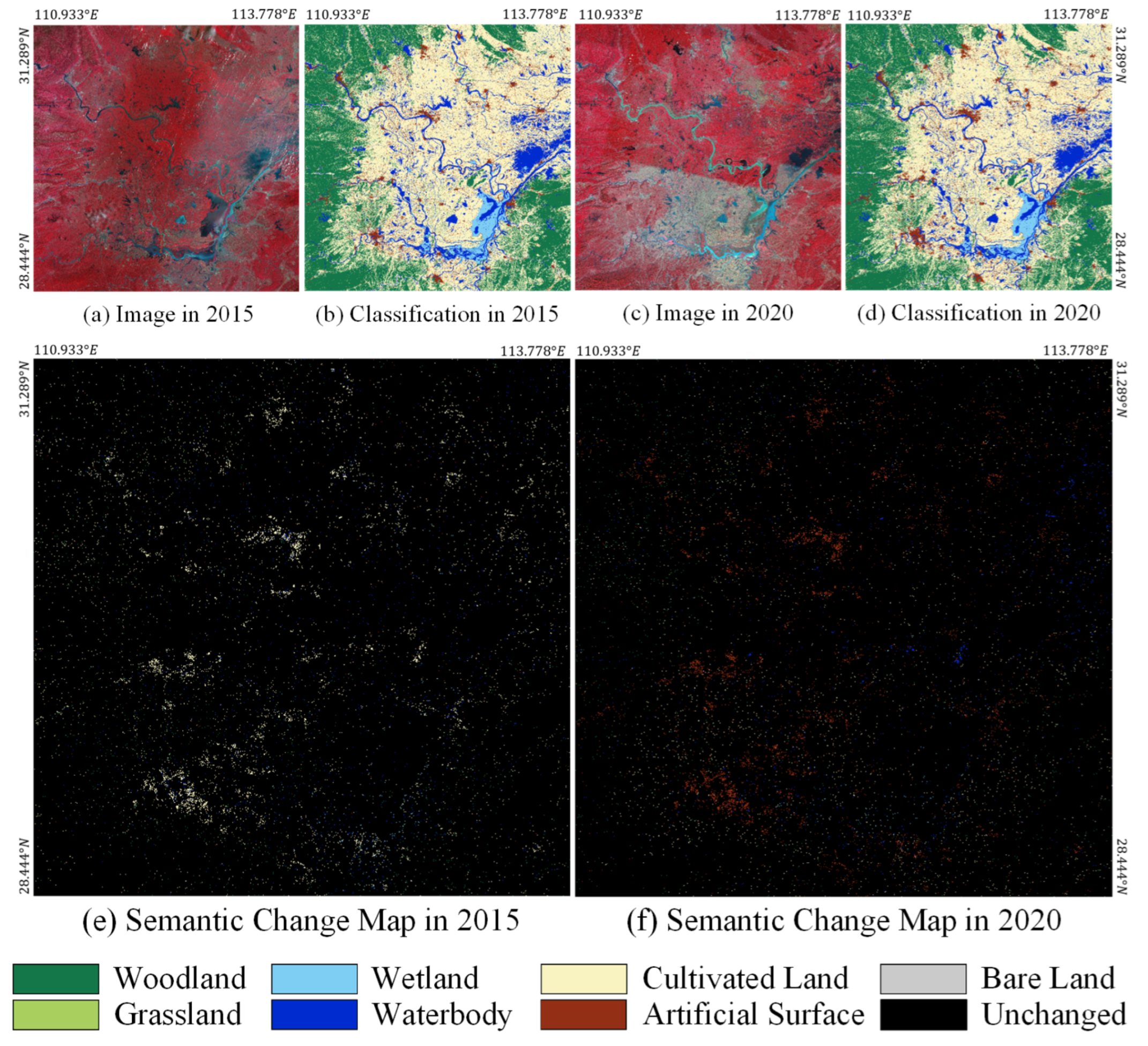
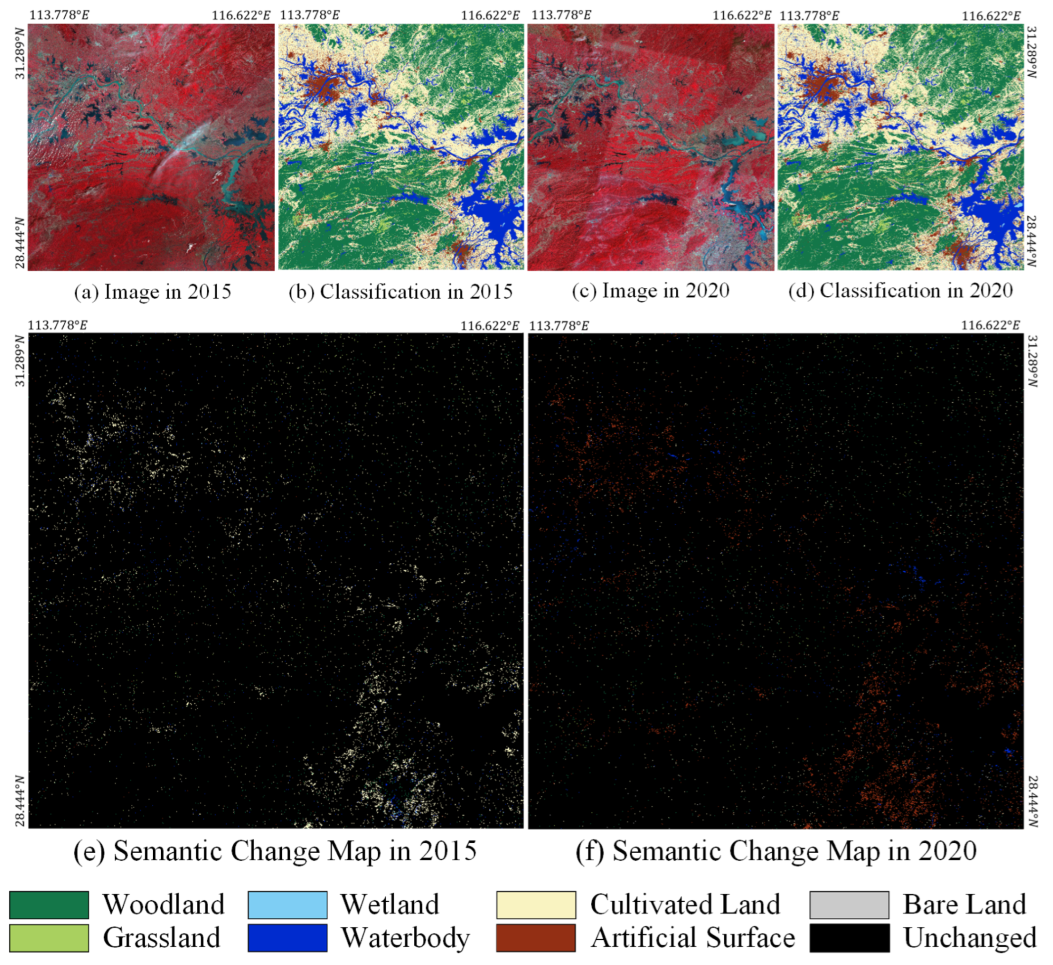
The landcover change in the whole study area from 2015 to 2020 is shown in Figure 12. The figure shows the landcover classification results in 2015, the landcover classification results in 2020, and the two-phase corresponding ground object classes in the changing area. The ground objects in Figure 12e become equivalent to the ground objects in Figure 12f. Table 11 is the category transition matrix of the two-phase landcover changes. It can be seen that from 2015 to 2020 in the study area, except for cultivated land and artificial surface, the area changes of other categories are very small. The area of cultivated land was significantly reduced, and the artificial surface area was significantly increased. In a more specific analysis, there is a small interchange between woodland and cultivated land. This is because there will be a small dynamic balance change at the boundaries. In addition, a small part of the woodland has been turned into artificial surface. The reason for this is the encroachment of some forest land by urban development. Wetlands are relatively stable, indicating that wetland protection policies have achieved practical results. The exchange of cultivated land and wetlands is also due to the similarity between paddy fields and waterbodies. A large area of cultivated land has become artificial surface, and the change is larger than in the previous ten years. It shows that the city expanded very rapidly from 2015 to 2020, occupying a large amount of cultivated land around the city, reflecting the acceleration of urbanization and the rapid development of the economic level. More details on these changes can be found in Appendix B.3.
4.4. Implications and Limitations
The PSNet proposed in this paper solves three critical problems encountered by the multi-temporal Landsat landcover changes. The first problem is the pseudo-changes caused by differences in color distribution. The second problem is the enhancement and suppression of true and false changes. The third problem is that multi-task networks cannot jointly optimize and constrain each other when performing change detection and semantic segmentation.
For the study of landcover changes, independent semantic segmentation of multi-temporal images is a mainstream method. This method is very sensitive to color differences between multi-temporal images, resulting in many pseudo-change errors in the results. However, the current method of remote sensing multi-temporal image change detection can only focus on the binary information of change and unchanged. It cannot obtain information on the mutual change process between categories. Therefore, a new idea is proposed to design a two-in-one single-task network for semantic segmentation and change detection to solve these three critical problems.
We add an additional encoder branch to the mainstream Siamese network for remote sensing change detection. The original two Siamese branches extract the image features of the two phases, respectively. Then, the data and labels of the third phase are introduced into the newly added additional encoder, which is used as prior knowledge to guide and constrain the feature learning of the original two Siamese branches. Under the constraints of prior knowledge, the two Siamese encoders are simplified from learning complete texture features to only learning their change information relative to the prior image. In the region that has not changed, the label of the a priori phase is directly brought in. Since the network learns two-phase change thresholds based on samples, this dramatically reduces the problem of pseudo-changes caused by color differences. At this time, PSNet adds two additional decoders to implement the multi-task semantic change.
In the Landsat image with a resolution of 30 m, most of the changed features are very small, maybe only one pixel wide. As a result, the distinction between true changes and false changes is not high enough. We redesigned the commonly used difference or concatenation operation and used the difference square to amplify the true change and reduce the false change. The optimized features are then weighted onto feature maps with complete semantic information. This way, pseudo-change errors that are difficult to eliminate can be suppressed. The kept complete semantic features can lay the foundation for the subsequent semantic change two-in-one single-task network.
When using multiple decoder branches to implement the tasks of change detection and semantic segmentation, only the features of the shallow encoder will be fused. However, the decoders are still relatively independent. Therefore, the multi-branch features at the end of the network cannot constrain each other for optimization, information cannot be shared, and even contradictory errors may occur. We combine multiple decoders into a single decoder that converts two-phase semantic segmentation samples into a single semantic change sample with joint labels. With the help of feature learning enhancement and change feature optimization of the prior knowledge branch and DEB module, the single-task network directly implements semantic change detection in one step and can learn complex change states. While improving the efficiency of multi-task learning, the single-task network also solves the risk of conflicting multiple decoders, significantly improving the accuracy and reliability of semantic change detection.
The change detection method with complete semantic information provides powerful support for multi-temporal landcover changes. The mutual change information extracted by PSNet provides data support for analyzing landcover classification and change. Based on the landcover change data, it is possible to further discover and explore phenomena, such as returning farmland to forests, wetland ecological protection, and urban expansion, and mine information, such as the status quo of social and economic development and policy decision making and planning. The PSNet proposed in this paper can quickly extract and analyze the landcover change information in large-scale and multi-temporal dimensions and has significant application value. Based on PSNet, we also conduct a detailed analysis of the large-scale multi-temporal Landsat landcover changes from 2005 to 2020. Urban expansion and the devouring of cultivated land are the most critical keywords obtained in the land cover change analysis.
Compared with mainstream semantic segmentation and change detection networks, the PSNet proposed in this paper provides a new problem-solving idea. The idea is the introduction of prior knowledge constraints, which significantly improves the accuracy and has more practical application value. However, this also brings certain limitations. When performing semantic change detection on two-phase images, the third-phase images and labels must be sacrificed. That is to say, at least three registered multi-temporal samples are required for model training. However, the more time phases there are, the more difficult it is to label samples. Therefore, while PSNet achieves higher accuracy, the workload of manual interpretation in the early stage is also higher than other mainstream algorithms. In future research, we will explore unpaired labels as prior knowledge to improve network accuracy, which may avoid manual labeling work in additional phases and reduce the workload and difficulty of preparatory work. We will also apply our proposed PSNet to single-band images and high-resolution images.
5. Conclusions
In this paper, we propose a prior semantic network for the Landsat semantic change task. Based on the dual-branch Siamese network, we add a prior knowledge encoder branch to solve the problem of pseudo-changes caused by color distribution differences. We design a difference enhancement block module to replace the common difference or concatenation operation and solve the problem of the enhancement and suppression of true and false changes. We propose a single-task PSNet, which combines multiple decoders into one decoder, solving the problem that features cannot be jointly optimized and mutually constrained in multi-task networks. Our proposed method achieves state-of-the-art performance on large-scale multi-temporal Landsat landcover change datasets, far exceeding other change detection and semantic segmentation networks. Based on PSNet, we conducted a specific analysis and discussion on the landcover changes in an area of central and southern China. The acceleration of urbanization construction and the acceleration of economic development are the two keywords we have found from the results of landcover changes over 15 years. This work has a particular value for sustainable development goals. In future research, we will study constraint learning on unpaired samples and generalize PSNet to more multi-temporal remote sensing data of different resolutions.
Author Contributions
X.Y. wrote the manuscript, designed the methodology, and conducted experiments; Y.B. and P.C. validated and analyzed the results; C.L. and K.L. preprocessed the data of the study area and made the datasets; Z.C. supervised the study and reviewed the manuscript. All authors have read and agreed to the published version of the manuscript.
Funding
This research was supported by the Strategic Priority Research Program of the Chinese Academy of Sciences under Grant No. XDA23100304.
Institutional Review Board Statement
Not applicable.
Informed Consent Statement
Not applicable.
Data Availability Statement
Not applicable.
Acknowledgments
The authors thank the editors and anonymous reviewers for their valuable comments, which greatly improved the quality of the paper.
Conflicts of Interest
The authors declare no conflict of interest.
Abbreviations
The following abbreviations are used in this manuscript:
| DCNN | deep convolutional neural network |
| DEB | difference enhancement block |
| F1 | F1 score |
| mF1 | mean F1 score |
| FN | false negative |
| FP | false positive |
| IoU | intersection over union |
| MT | multi-task |
| NDBI | normalized difference built-up index |
| NDVI | normalized difference vegetation index |
| NDWI | normalized difference water index |
| OA | overall accuracy |
| OLI | operational land imager |
| PSNet | prior semantic network |
| ReLU | rectified linear unit |
| SiamUNet | Siamese UNet |
| ST | single-task |
| TM | thematic mapper |
| TN | true negative |
| TP | true positive |
Appendix A. More Comparisons for Experiments
Appendix A.1. More Comparisons for Binary Change Detection
Figure A1 is a comparison chart of the change detection results. In the first group, FC-Siam-diff and DDCNN cannot detect the changing regions normally. FC-EF and FC-Siam-conc have missed many obvious detections, while DSIFN, CDNet, and UNet++MSOF have many false detections. Baseline SiamUNet also has false detections, but they are relatively less. PSNet, assisted by prior knowledge, further reduces the false detection rate. The DEB module is over-filtered. The change detection results of the integrated decoder of PSNet-ST have the highest agreement with the label and the best performance. In the second group, none of FC-Siam-diff, DDCNN, DSIFN, CDNet, or UNet++MSOF can detect the change correctly. Although FC-EF and FC-Siam-conc have no obvious false detections, the phenomenon of missed detection is serious. Due to the absence of prior knowledge constraints, baseline SiamUNet performs similarly to mainstream networks. Most areas of the city are falsely detected as changing areas. PSNet dramatically reduces the false detection rate. With the help of the DEB module, the change detection results are very close to the ground truth labels, but there are some cases of missed detections. PSNet-ST with the integrated decoder can combine the advantages of PSNet and PSNet-DEB, and its change detection performance is the best.
Figure A1.
Comparison of the binary change detection results between PSNet and other methods: (a) Images in 2005. (b) Images in 2010. (c) Labels in 2005. (d) Labels in 2010. (e) Binary change labels. Inference result of (f) the FC-EF, (g) the FC-Siam-diff, (h) the FC-Siam-conc, (i) the DSIFN, (j) the DDCNN, (k) the CDNet, (l) UNet++MSOF, (m) the SiamUNet, (n) our proposed PSNet, (o) our proposed PSNet-DEB, and (p) our proposed PSNet-ST.

Appendix A.2. More Comparisons for Semantic Change Detection
Figure A2 is a comparison chart of the semantic change detection results. The main change is that cultivated land becomes the artificial surface as the city expands. The results of SiamUNet extracted many unchanged artificial surfaces as changed regions. The results of PSNet take a small part of the cultivated land as the changing area, but due to the effect of prior knowledge, the false detection rate has been greatly reduced. The results of PSNet-DEB and PSNet-ST are both close to the labels, and the semantic change results of PSNet-ST are more refined and detailed. It also reflects mutual assistance and guidance advantages after combining semantic segmentation and change detection tasks.
Figure A2.
Comparison of the semantic change detection results between the SiamUNet and PSNet series networks. (a) Images. (b) Labels. Inference result of (c) the SiamUNet, (d) our proposed PSNet, (e) our proposed PSNet-DEB, and (f) our proposed PSNet-ST.
Figure A2.
Comparison of the semantic change detection results between the SiamUNet and PSNet series networks. (a) Images. (b) Labels. Inference result of (c) the SiamUNet, (d) our proposed PSNet, (e) our proposed PSNet-DEB, and (f) our proposed PSNet-ST.

Appendix B. Detailed Discussion for Landcover Change
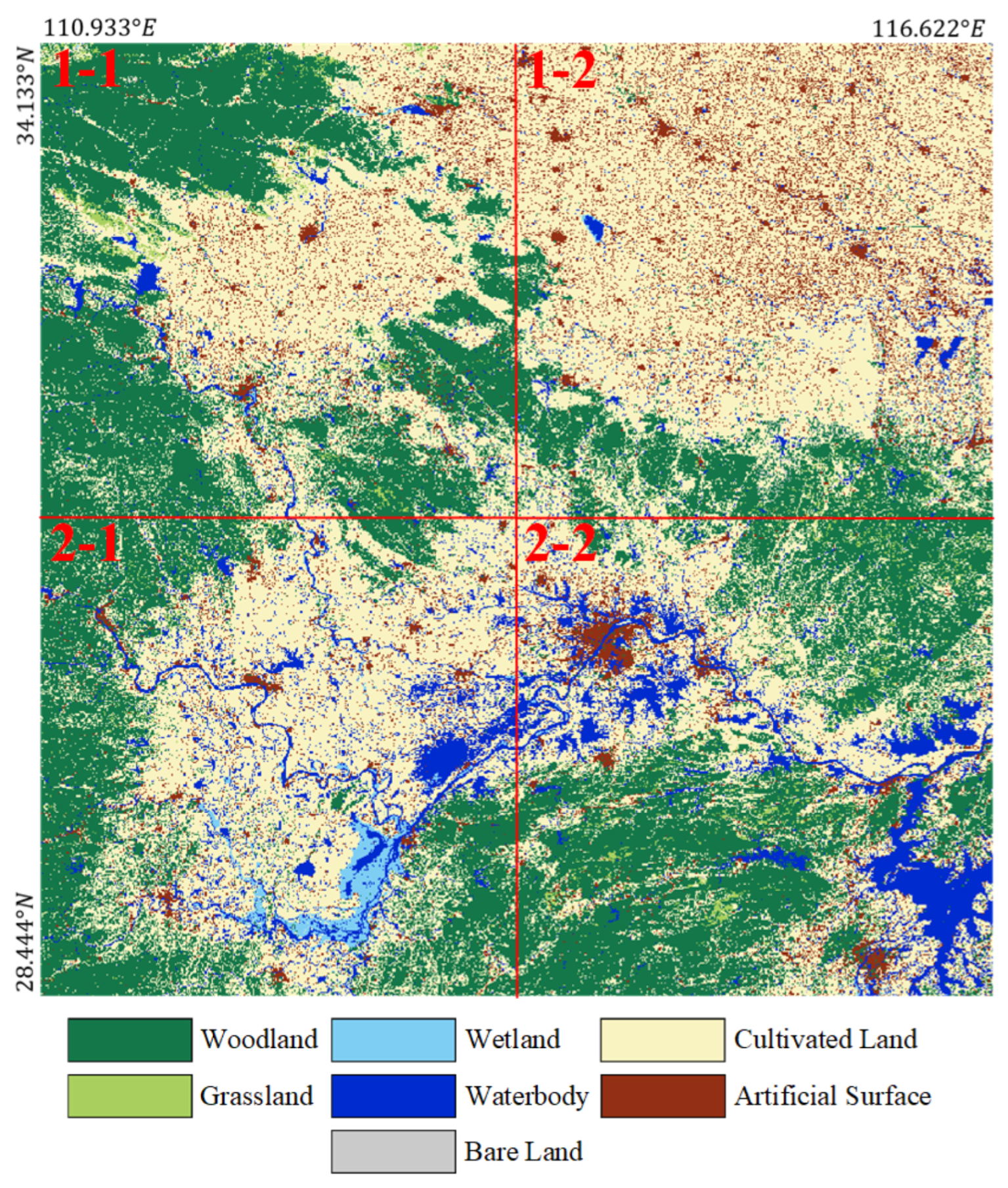
Since the changing area of the adjacent two-phase images only accounts for about 6% of the total study area, most change patches are very small. The whole study area is divided into four small blocks of 10,240 × 10,240 pixels displayed separately. As shown in Figure A3, each small block is numbered 1-1, 1-2, 2-1, and 2-2. The actual area covered by each small image is 90,000 .
Figure A3.
Geographical distribution diagram of four small blocks in study area. IDs 1-1, 1-2, 2-1, and 2-2.
Figure A3.
Geographical distribution diagram of four small blocks in study area. IDs 1-1, 1-2, 2-1, and 2-2.

Appendix B.1. Detailed Analysis of Landcover Change from 2005 to 2010
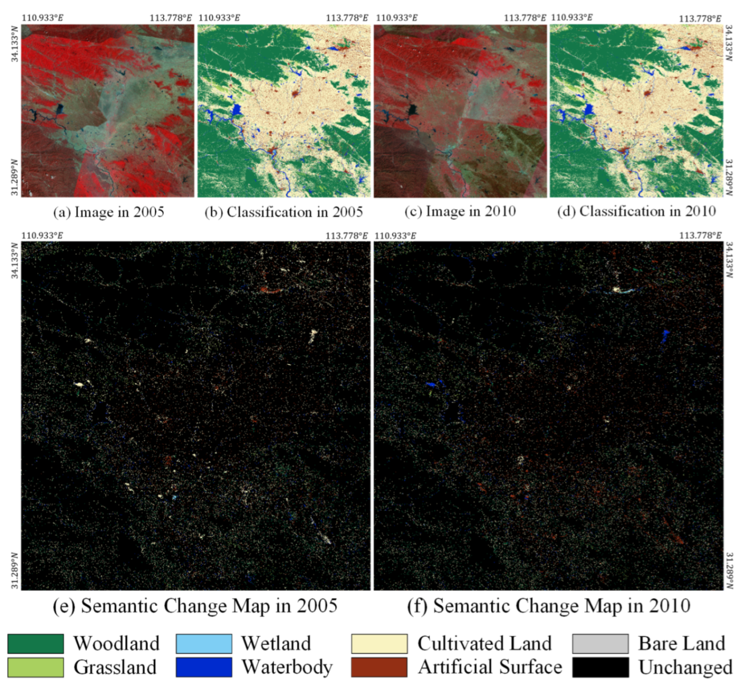
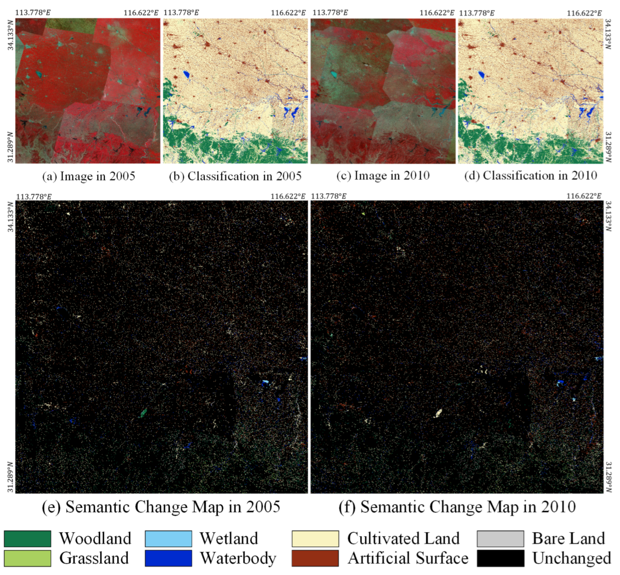
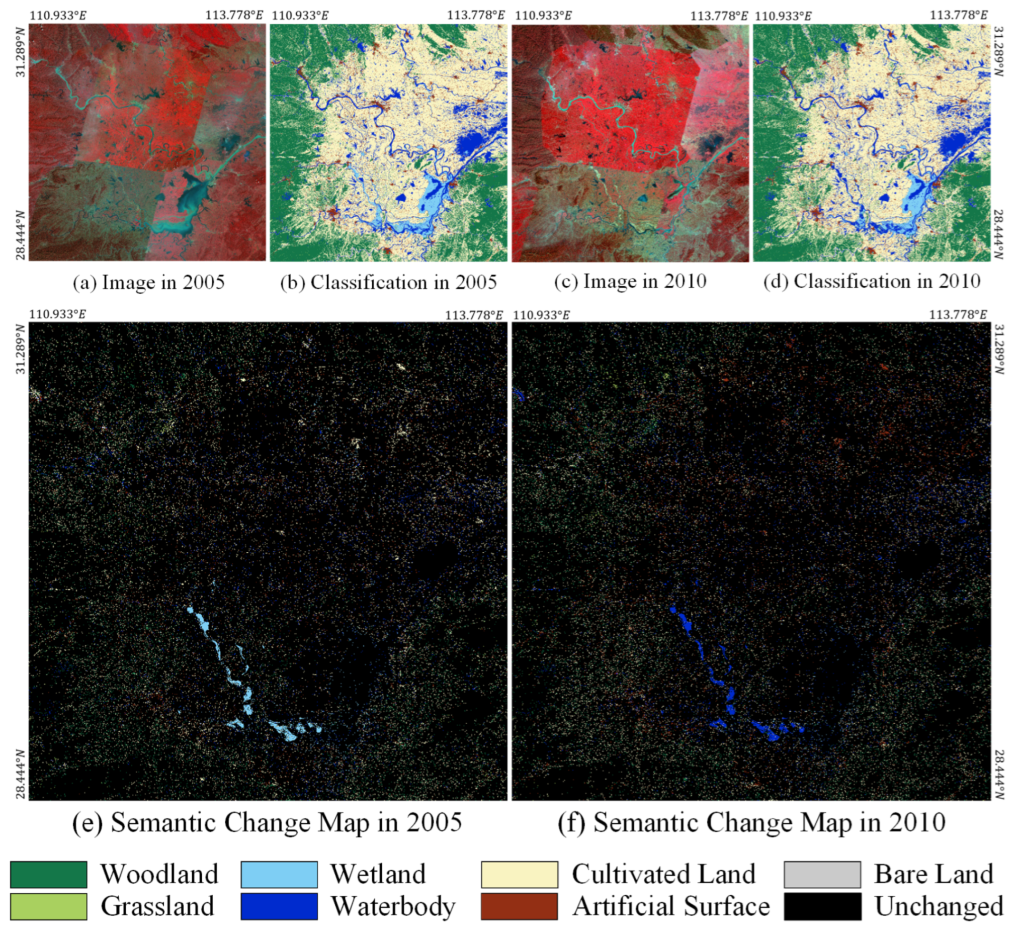
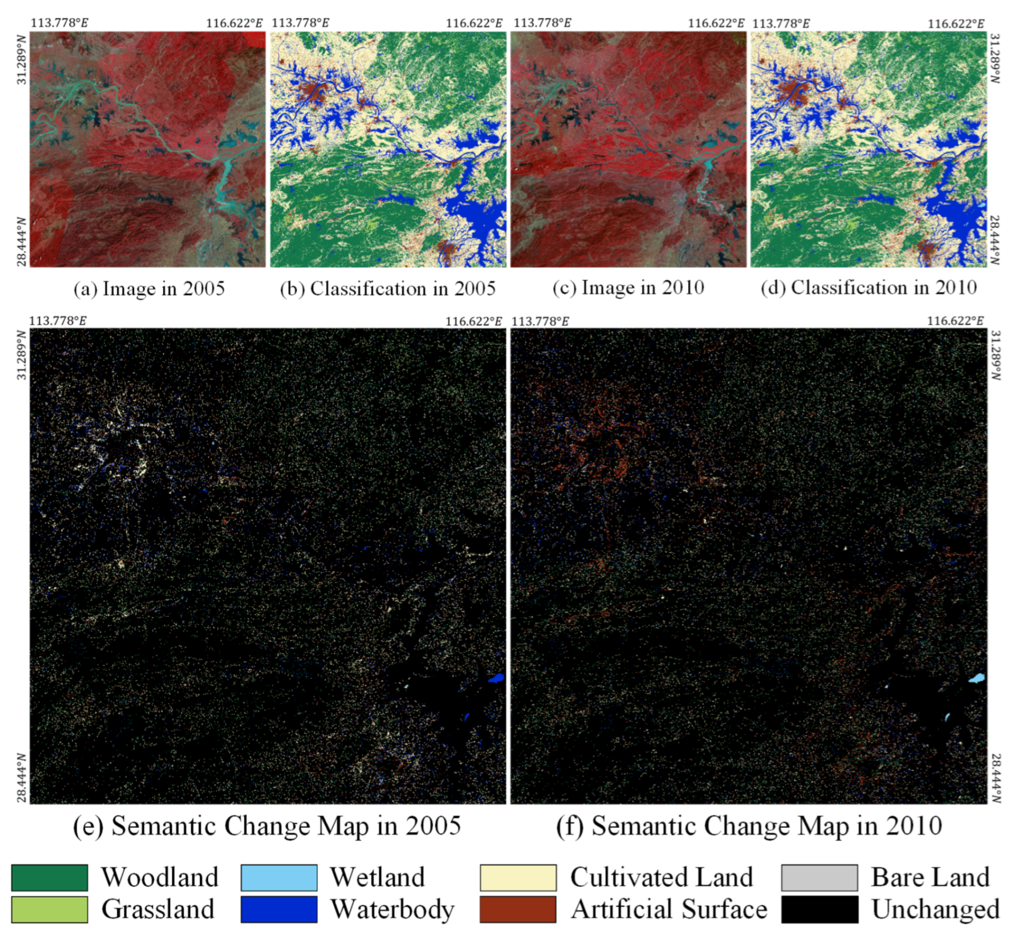
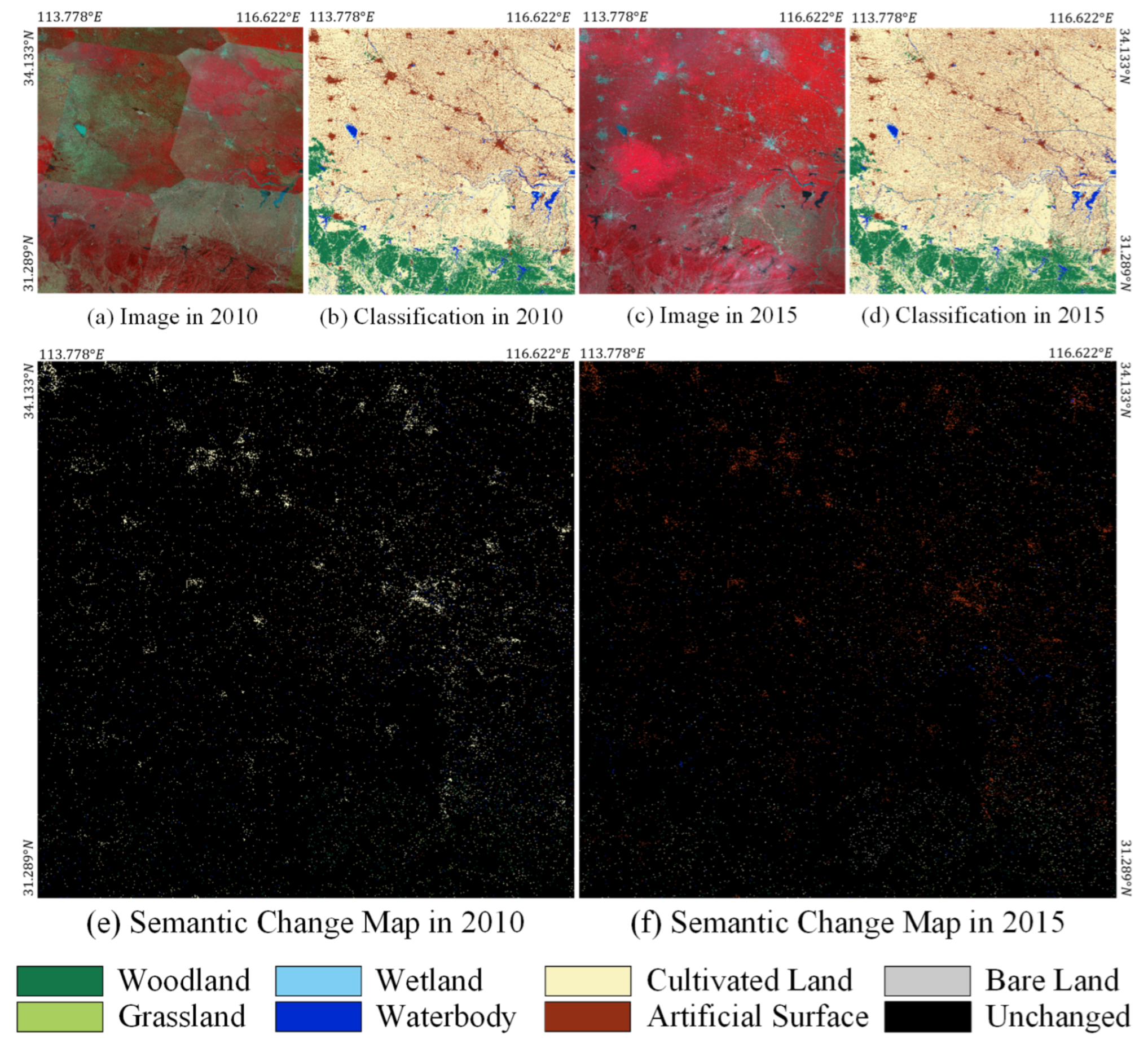
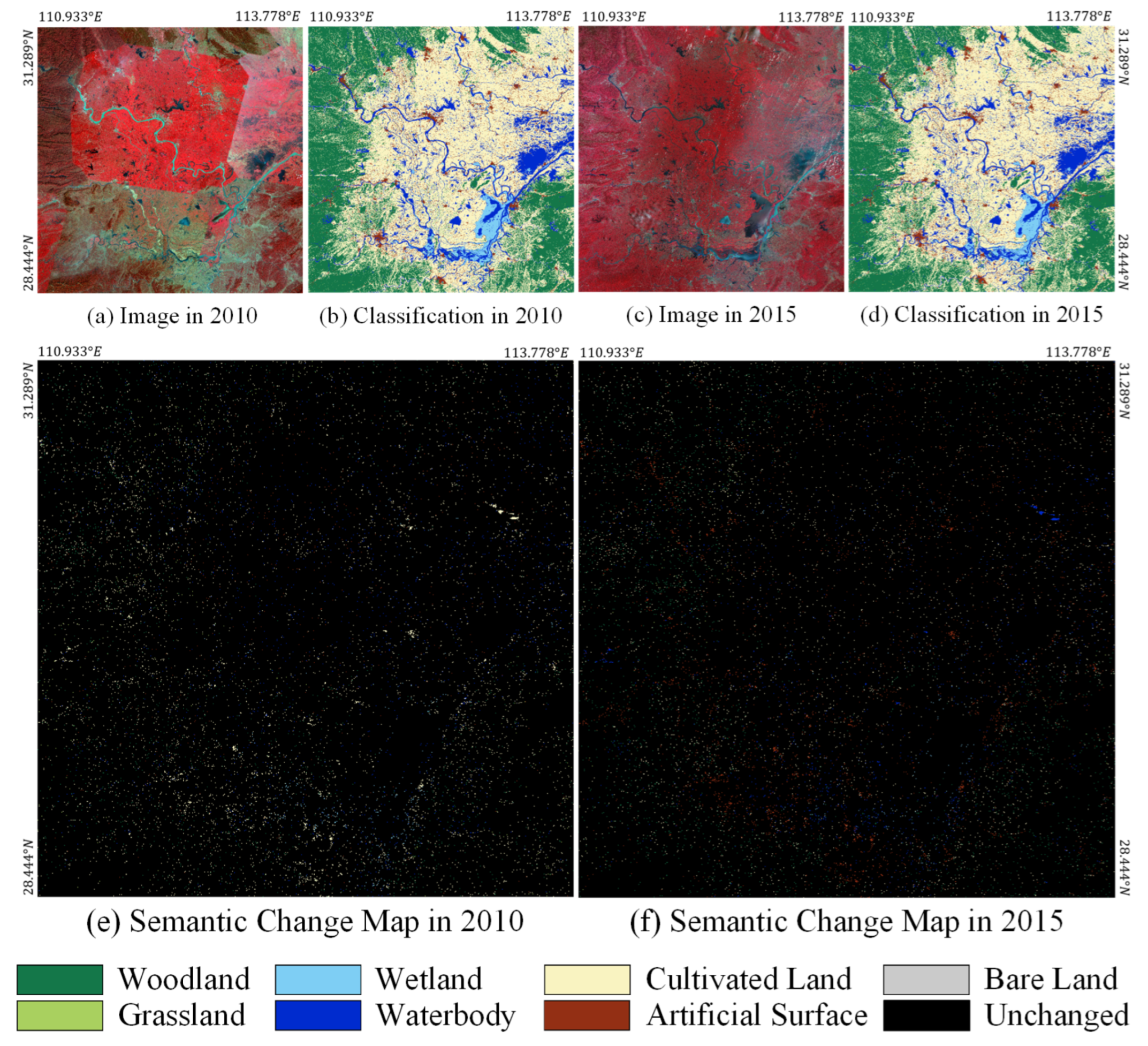
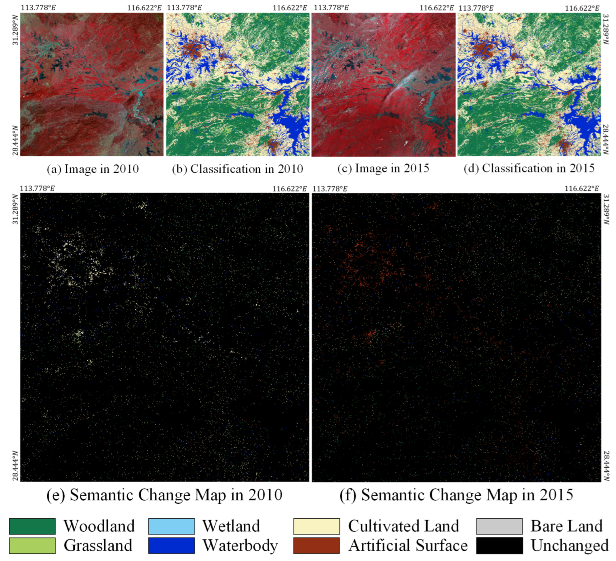
To show the geographical distribution of the changes’ details, Figure A4 shows the large-scale details in block 1-1 of the study area. It can be seen that two large cultivated land became waterbodies. From the image, these two areas show the increase in the reservoir area or the newly built reservoir. A piece of the artificial surface has been turned into cultivated land and wetlands because this area is planned as a wetland ecological protection area. The other obvious changes are the transformation of cultivated land into artificial surface. This change is basically distributed around towns and cities. The change range is not large, and the distribution is scattered, which aligns with the urban development trend. Figure A5 shows the large-scale details in block 1-2 of the study area. It can be seen that there is a piece of woodland that has been turned into cultivated land, where excessive deforestation has occurred. There is an exchange phenomenon between a waterbody and a wetland. This is because the location is a reservoir and a wetland protection area. Part of the water area is shallow, and the difference is not obvious enough. Figure A6 shows the large-scale details in block 2-1 of the study area. It can be seen that a large piece of wetland has become a waterbody. This area is the Dongting Lake area. In the season when the water volume is large, the depth of the wetland becomes deeper, and it looks like a waterbody. Most of Dongting Lake is shallow, so wetlands dominate the waterbody. Exchanges between wetlands and waterbodies occur in different seasons. In addition, the most obvious change is the expansion of the city and the annexation of the surrounding cultivated land. Figure A7 shows the large-scale details in block 2-2 of the study area. It can be seen that there is an area in which the artificial surface has occupied a large amount of cultivated land. This area is Wuhan City, which shows that the development speed of the city is very fast. Another small piece of waterbody became a wetland. This area is located around Poyang Lake. It is normal for a waterbody to turn into a wetland during the dry season.
Figure A4.
The landcover change map in block 1-1 from 2005 to 2010. (a) Image in 2005. (b) Classification result in 2005. (c) Image in 2010. (d) Classification result in 2010. (e) Semantic change map in 2005. (f) Semantic change map in 2010.
Figure A4.
The landcover change map in block 1-1 from 2005 to 2010. (a) Image in 2005. (b) Classification result in 2005. (c) Image in 2010. (d) Classification result in 2010. (e) Semantic change map in 2005. (f) Semantic change map in 2010.

Figure A5.
The landcover change map in block 1-2 from 2005 to 2010. (a) Image in 2005. (b) Classification result in 2005. (c) Image in 2010. (d) Classification result in 2010. (e) Semantic change map in 2005. (f) Semantic change map in 2010.
Figure A5.
The landcover change map in block 1-2 from 2005 to 2010. (a) Image in 2005. (b) Classification result in 2005. (c) Image in 2010. (d) Classification result in 2010. (e) Semantic change map in 2005. (f) Semantic change map in 2010.

Figure A6.
The landcover change map in block 2-1 from 2005 to 2010. (a) Image in 2005. (b) Classification result in 2005. (c) Image in 2010. (d) Classification result in 2010. (e) Semantic change map in 2005. (f) Semantic change map in 2010.
Figure A6.
The landcover change map in block 2-1 from 2005 to 2010. (a) Image in 2005. (b) Classification result in 2005. (c) Image in 2010. (d) Classification result in 2010. (e) Semantic change map in 2005. (f) Semantic change map in 2010.

Figure A7.
The landcover change map in block 2-2 from 2005 to 2010. (a) Image in 2005. (b) Classification result in 2005. (c) Image in 2010. (d) Classification result in 2010. (e) Semantic change map in 2005. (f) Semantic change map in 2010.
Figure A7.
The landcover change map in block 2-2 from 2005 to 2010. (a) Image in 2005. (b) Classification result in 2005. (c) Image in 2010. (d) Classification result in 2010. (e) Semantic change map in 2005. (f) Semantic change map in 2010.

Appendix B.2. Detailed Analysis of Landcover Change from 2010 to 2015
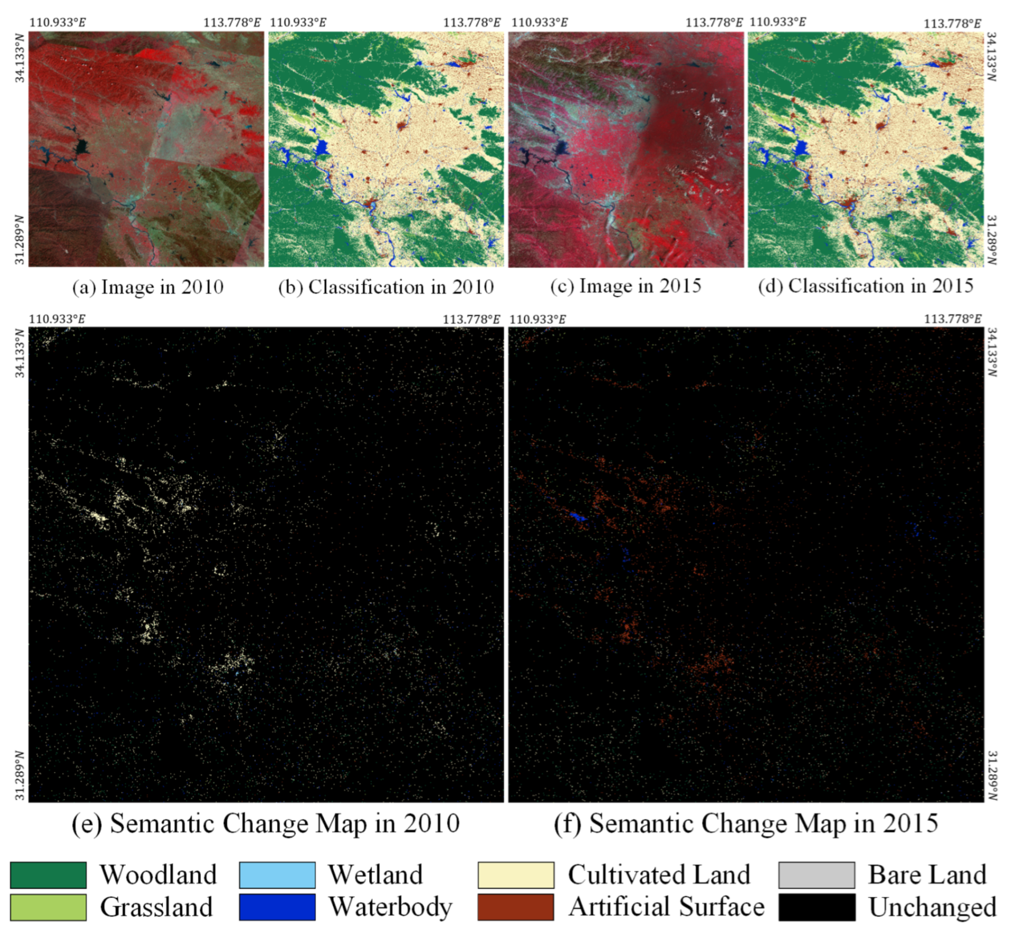
To show the geographical distribution of the changes’ details, Figure A8 shows the large-scale details in block 1-1 of the study area. It can be seen that a large amount of cultivated land has become artificial surface, and the speed of urbanization has been greatly accelerated. A few small pieces of cultivated land have become waterbodies, mainly because the water storage capacity of the reservoir has increased, and the original cultivated land has been adjusted for the reservoir. Figure A9 shows the large-scale details in block 1-2 of the study area. It can be seen that the most noticeable change is that the artificial surface has encroached on a large amount of surrounding cultivated land, which also reflects the speed of urbanization. Figure A10 shows the large-scale details in block 2-1 of the study area. Changes in this area are small. Since there are no megacities, there is an increase in artificial surfaces, but not very significant. In addition, there is a small increase in the waterbody, indicating that the water volume has increased in this changing region. Figure A11 shows the large-scale details in block 2-2 of the study area. It can be seen that the urban scale of Wuhan, a large city, is still expanding rapidly. On the whole, the changes in natural features from 2010 to 2015 were small, and the artificial surface expanded significantly. It shows that the urban development in the past five years is the main factor in landcover change.
Figure A8.
The landcover change map in block 1-1 from 2010 to 2015. (a) Image in 2010. (b) Classification result in 2010. (c) Image in 2015. (d) Classification result in 2015. (e) Semantic change map in 2010. (f) Semantic change map in 2015.
Figure A8.
The landcover change map in block 1-1 from 2010 to 2015. (a) Image in 2010. (b) Classification result in 2010. (c) Image in 2015. (d) Classification result in 2015. (e) Semantic change map in 2010. (f) Semantic change map in 2015.

Figure A9.
The landcover change map in block 1-2 from 2010 to 2015. (a) Image in 2010. (b) Classification result in 2010. (c) Image in 2015. (d) Classification result in 2015. (e) Semantic change map in 2010. (f) Semantic change map in 2015.
Figure A9.
The landcover change map in block 1-2 from 2010 to 2015. (a) Image in 2010. (b) Classification result in 2010. (c) Image in 2015. (d) Classification result in 2015. (e) Semantic change map in 2010. (f) Semantic change map in 2015.

Figure A10.
The landcover change map in block 2-1 from 2010 to 2015. (a) Image in 2010. (b) Classification result in 2010. (c) Image in 2015. (d) Classification result in 2015. (e) Semantic change map in 2010. (f) Semantic change map in 2015.
Figure A10.
The landcover change map in block 2-1 from 2010 to 2015. (a) Image in 2010. (b) Classification result in 2010. (c) Image in 2015. (d) Classification result in 2015. (e) Semantic change map in 2010. (f) Semantic change map in 2015.

Figure A11.
The landcover change map in block 2-2 from 2010 to 2015. (a) Image in 2010. (b) Classification result in 2010. (c) Image in 2015. (d) Classification result in 2015. (e) Semantic change map in 2010. (f) Semantic change map in 2015.
Figure A11.
The landcover change map in block 2-2 from 2010 to 2015. (a) Image in 2010. (b) Classification result in 2010. (c) Image in 2015. (d) Classification result in 2015. (e) Semantic change map in 2010. (f) Semantic change map in 2015.

Appendix B.3. Detailed Analysis of Landcover Change from 2015 to 2020
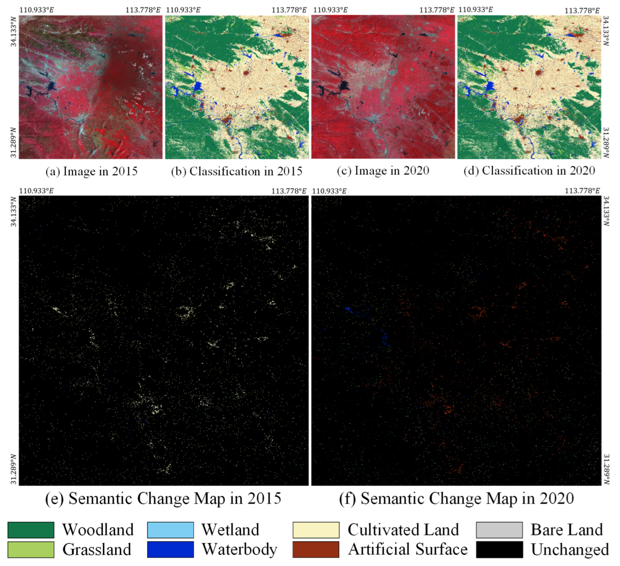
To show the geographical distribution of the changes’ details, Figure A12 shows the large-scale details in block 1-1 of the study area. It can be seen that there are mainly two changes. One is that the cultivated land around the town has become artificial surface, representing the expansion of the city. The other is that part of the cultivated land around the waterbody is swallowed up. This is because the water storage capacity of the reservoir increased, so the area of the waterbody expanded. Figure A13, Figure A14 and Figure A15 show the large-scale details in blocks 1-2, 2-1, and 2-2 of the study area, respectively. The changes are basically similar to block 1-1, and the urban expansion is pronounced. It shows that the leading development tone from 2015 to 2020 is urbanization construction, and the soil occupied during urban growth is basically cultivated land. It is also because, in most cases, towns are surrounded by cultivated land in the countryside. If the city is surrounded by woodland, the corresponding woodland will be converted into artificial surface. This trend exists in the study area, but it is much smaller than the area of cultivated land converted into artificial surface.
Figure A12.
The landcover change map in block 1-1 from 2015 to 2020. (a) Image in 2015. (b) Classification result in 2015. (c) Image in 2020. (d) Classification result in 2020. (e) Semantic change map in 2015. (f) Semantic change map in 2020.
Figure A12.
The landcover change map in block 1-1 from 2015 to 2020. (a) Image in 2015. (b) Classification result in 2015. (c) Image in 2020. (d) Classification result in 2020. (e) Semantic change map in 2015. (f) Semantic change map in 2020.

Figure A13.
The landcover change map in block 1-2 from 2015 to 2020. (a) Image in 2015. (b) Classification result in 2015. (c) Image in 2020. (d) Classification result in 2020. (e) Semantic change map in 2015. (f) Semantic change map in 2020.
Figure A13.
The landcover change map in block 1-2 from 2015 to 2020. (a) Image in 2015. (b) Classification result in 2015. (c) Image in 2020. (d) Classification result in 2020. (e) Semantic change map in 2015. (f) Semantic change map in 2020.

Figure A14.
The landcover change map in block 2-1 from 2015 to 2020. (a) Image in 2015. (b) Classification result in 2015. (c) Image in 2020. (d) Classification result in 2020. (e) Semantic change map in 2015. (f) Semantic change map in 2020.
Figure A14.
The landcover change map in block 2-1 from 2015 to 2020. (a) Image in 2015. (b) Classification result in 2015. (c) Image in 2020. (d) Classification result in 2020. (e) Semantic change map in 2015. (f) Semantic change map in 2020.

Figure A15.
The landcover change map in block 2-2 from 2015 to 2020. (a) Image in 2015. (b) Classification result in 2015. (c) Image in 2020. (d) Classification result in 2020. (e) Semantic change map in 2015. (f) Semantic change map in 2020.
Figure A15.
The landcover change map in block 2-2 from 2015 to 2020. (a) Image in 2015. (b) Classification result in 2015. (c) Image in 2020. (d) Classification result in 2020. (e) Semantic change map in 2015. (f) Semantic change map in 2020.

Appendix B.4. Analysis of Landcover Change in Fifteen Years
From Section 4.1, Section 4.2 and Section 4.3, it can be found that in the study area, from 2005 to 2020, the most obvious change is that a large amount of cultivated land has become artificial surface. The reduced area of cultivated land is approximately equal to the increased area of artificial surface, which is in line with the fact that the surrounding cultivated land is occupied during urban expansion. In the early days, the waterbody area increased more, which was related to the construction of water conservancy projects such as reservoirs in the area. The changes in other categories are not obvious.
We have accumulated the changes in the past 15 years, and the specific changes in landcover are shown in Table A1. The changing area within the study area amounted to 28,985.68 . The woodland increased by 232.62 and has a small dynamic balance changed with grassland, waterbody, cultivated land, and artificial surface. Among them, the mutual change with cultivated land is the most because there are cases of returning farmland to forest and cutting down trees for reclamation in this area. Grassland has decreased by 145.85 and has a small dynamic balance changed with woodland and cultivated land. Affected by the season, the grass on the ground will appear in the image after the trees have fallen, and the grass will be blocked when the leaves are dense. Therefore, there will be changes in the dynamic balance between woodland and grassland. Similarly, weeds may grow when cultivated land is idle, and cultivated land can be restored after weeding. Therefore, there will be exchanges between grassland and cultivated land. Wetlands decreased by 360.58 , mainly turning into waterbodies. When the water storage capacity of wetlands increases, wetlands may become lakes or reservoirs. In addition, there is a small amount of mutual change between wetlands and woodland, cultivated land, and artificial surfaces. This is because wetlands are relatively fragile and may become other categories if they are not well protected. The waterbody area increased by 28.4 . It is very small. However, in the past 15 years, the waterbody has been in a state of dynamic change. The mutual change between waterbody and woodland areas indicates that the newly added reservoir in this area will submerge some woodland. At the same time, trees will become the main features in some dry water areas. The exchange between waterbodies and cultivated land can also reflect the cultivated land being submerged and newly reclaimed cultivated land brought about by the construction of new reservoirs and the drying up of waters. There are also minor changes in the waterbody and artificial surface because the small villages and towns will be relocated when the reservoir is newly built. The cultivated land decreased by 7893.78 , mainly because the artificial surface gradually swallowed it up in urbanization. There is basically a state of balanced exchange between cultivated land and other categories. The artificial surface has increased by 8083.83 . The speed of urbanization also reflects the outstanding economic level in the past 15 years. The newly added artificial surface area has reached one-third of the unchanged artificial surface area. In other words, the urban area has increased by about 34.1% in 15 years. The bare land area increased by 55.37 , with relatively little change between categories. Bare land accounts for a small proportion, and due to conditions such as imaging seasons and human factors such as urban planning and construction, bare land will appear or disappear briefly.

Table A1.
Landcover change statistics in the past 15 years. (Unit: square kilometers).
| Woodland | Grassland | Wetland | Waterbody | Cultivated Land | Artificial Surface | Bare Land | Total Out | |
|---|---|---|---|---|---|---|---|---|
| Woodland | 117,813.68 | 381.17 | 3.10 | 270.82 | 4112.36 | 643.07 | 78.87 | 5489.40 |
| Grassland | 508.33 | 3532.18 | 0.25 | 16.03 | 219.32 | 16.59 | 4.44 | 764.95 |
| Wetland | 26.53 | 1.02 | 2232.25 | 424.07 | 71.03 | 43.02 | 1.70 | 567.38 |
| Waterbody | 330.94 | 9.09 | 135.38 | 24,587.92 | 1692.60 | 598.83 | 26.08 | 2792.92 |
| Cultivated Land | 4549.51 | 218.68 | 55.46 | 1870.65 | 176,007.48 | 9600.65 | 77.70 | 16,372.67 |
| Artificial Surface | 262.49 | 6.79 | 12.50 | 208.82 | 2334.08 | 23,665.93 | 20.13 | 2844.81 |
| Bare Land | 44.21 | 2.34 | 0.11 | 30.93 | 49.48 | 26.48 | 662.25 | 153.55 |
| Total In | 5722.02 | 619.10 | 206.79 | 2821.32 | 8478.88 | 10,928.64 | 208.92 | 28,985.68 |
| Total Change | 232.62 | −145.85 | −360.58 | 28.40 | −7893.78 | 8083.83 | 55.37 | - |
Figure A16 shows the change details in the study area from 2005 to 2020. It can be seen that the transformation of cultivated land into artificial surface is the most critical change, and it is mainly distributed around towns and cities. It is consistent with the law of urban expansion. At the same time, due to the newly built reservoirs and other water conservancy projects in this area and the protection policy of Dongting Lake, some cases of cultivated land turning into waterbodies can also be found in the figure. Combining the data and figures for landcover changes from 2005 to 2020, we can conclude that urbanization is the core keyword in the study area. Urbanization has an apparent relationship with social and economic development. The speed of urban expansion is becoming faster and faster, and we should pay attention to the occupation of cultivated land in the process of expansion because cultivated land is directly related to food. Wetlands and waterbodies are directly related to the ecological environment. How to protect wetlands is a significant issue that decision-making departments cannot ignore. As the main features of greening, woodland and grassland also need to be protected and increased as much as possible to achieve sustainable development goals.
Figure A16.
The landcover change map in the past 15 years. (a) Image in 2005. (b) Classification result in 2005. (c) Image in 2020. (d) Classification result in 2020. (e) Semantic change map in 2005. (f) Semantic change map in 2020.
Figure A16.
The landcover change map in the past 15 years. (a) Image in 2005. (b) Classification result in 2005. (c) Image in 2020. (d) Classification result in 2020. (e) Semantic change map in 2005. (f) Semantic change map in 2020.

References
- Ma, L.; Liu, Y.; Zhang, X.; Ye, Y.; Yin, G.; Johnson, B.A. Deep learning in remote sensing applications: A meta-analysis and review. ISPRS J. Photogramm. Remote Sens. 2019, 152, 166–177. [Google Scholar] [CrossRef]
- Hansen, M.C.; Loveland, T.R. A review of large area monitoring of land cover change using Landsat data. Remote Sens. Environ. 2012, 122, 66–74. [Google Scholar] [CrossRef]
- Feddema, J.J.; Oleson, K.W.; Bonan, G.B.; Mearns, L.O.; Buja, L.E.; Meehl, G.A.; Washington, W.M. The importance of land-cover change in simulating future climates. Science 2005, 310, 1674–1678. [Google Scholar] [CrossRef] [PubMed] [Green Version]
- Lepers, E.; Lambin, E.F.; Janetos, A.C.; DeFries, R.; Achard, F.; Ramankutty, N.; Scholes, R.J. A synthesis of information on rapid land-cover change for the period 1981–2000. BioScience 2005, 55, 115–124. [Google Scholar] [CrossRef]
- Evans, T.P.; Manire, A.; De Castro, F.; Brondizio, E.; McCracken, S. A dynamic model of household decision-making and parcel level landcover change in the eastern Amazon. Ecol. Model. 2001, 143, 95–113. [Google Scholar] [CrossRef]
- Rogan, J.; Miller, J.; Stow, D.; Franklin, J.; Levien, L.; Fischer, C. Land-cover change monitoring with classification trees using Landsat TM and ancillary data. Photogramm. Eng. Remote Sens. 2003, 69, 793–804. [Google Scholar] [CrossRef] [Green Version]
- Ma, Y.; Wu, H.; Wang, L.; Huang, B.; Ranjan, R.; Zomaya, A.; Jie, W. Remote sensing big data computing: Challenges and opportunities. Future Gener. Comput. Syst. 2015, 51, 47–60. [Google Scholar] [CrossRef] [Green Version]
- Zhang, B.; Wu, Y.; Zhao, B.; Chanussot, J.; Hong, D.; Yao, J.; Gao, L. Progress and challenges in intelligent remote sensing satellite systems. IEEE J. Sel. Top. Appl. Earth Obs. Remote Sens. 2022, 15, 1814–1822. [Google Scholar] [CrossRef]
- Zhang, B. Remotely sensed big data era and intelligent information extraction. Geomat. Inf. Sci. Wuhan Univ. 2018, 43, 1861–1871. [Google Scholar]
- Zhang, B.; Chen, Z.; Peng, D.; Benediktsson, J.A.; Liu, B.; Zou, L.; Li, J.; Plaza, A. Remotely sensed big data: Evolution in model development for information extraction [point of view]. Proc. IEEE 2019, 107, 2294–2301. [Google Scholar] [CrossRef]
- Bhandari, A.; Kumar, A.; Singh, G. Feature extraction using Normalized Difference Vegetation Index (NDVI): A case study of Jabalpur city. Procedia Technol. 2012, 6, 612–621. [Google Scholar] [CrossRef]
- Xing, D.P. One Method of Urban Land Covers Information Extraction. In Proceedings of the Applied Mechanics and Materials, Hong Kong, China, 17–18 August 2013; Trans Tech Publications: Zurich, Switzerland, 2013; Volume 380, pp. 4011–4014. [Google Scholar]
- Xu, H. Modification of normalised difference water index (NDWI) to enhance open water features in remotely sensed imagery. Int. J. Remote Sens. 2006, 27, 3025–3033. [Google Scholar] [CrossRef]
- Wei, W.; Chen, X.; Ma, A. Object-oriented information extraction and application in high-resolution remote sensing image. In Proceedings of the 2005 IEEE International Geoscience and Remote Sensing Symposium, IGARSS’05, Seoul, Korea, 25–29 July 2005; Volume 6, pp. 3803–3806. [Google Scholar]
- Lowe, D.G. Distinctive image features from scale-invariant keypoints. Int. J. Comput. Vis. 2004, 60, 91–110. [Google Scholar] [CrossRef]
- Rublee, E.; Rabaud, V.; Konolige, K.; Bradski, G. ORB: An efficient alternative to SIFT or SURF. In Proceedings of the 2011 International Conference on Computer Vision, Washington, DC, USA, 6–13 November 2011; pp. 2564–2571. [Google Scholar]
- Pal, M. Ensemble of support vector machines for land cover classification. Int. J. Remote Sens. 2008, 29, 3043–3049. [Google Scholar] [CrossRef]
- Hayes, M.M.; Miller, S.N.; Murphy, M.A. High-resolution landcover classification using Random Forest. Remote Sens. Lett. 2014, 5, 112–121. [Google Scholar]
- Kussul, N.N.; Lavreniuk, N.S.; Shelestov, A.Y.; Yailymov, B.Y.; Butko, I.N. Land cover changes analysis based on deep machine learning technique. J. Autom. Inf. Sci. 2016, 48, 42–54. [Google Scholar] [CrossRef]
- LeCun, Y.; Bengio, Y.; Hinton, G. Deep learning. Nature 2015, 521, 436–444. [Google Scholar] [CrossRef]
- Zhu, X.X.; Tuia, D.; Mou, L.; Xia, G.S.; Zhang, L.; Xu, F.; Fraundorfer, F. Deep learning in remote sensing: A comprehensive review and list of resources. IEEE Geosci. Remote Sens. Mag. 2017, 5, 8–36. [Google Scholar] [CrossRef] [Green Version]
- Lv, Z.; Liu, T.; Benediktsson, J.A.; Falco, N. Land cover change detection techniques: Very-high-resolution optical images: A review. IEEE Geosci. Remote Sens. Mag. 2021, 10, 44–63. [Google Scholar] [CrossRef]
- Lambin, E.F.; Geist, H.J.; Lepers, E. Dynamics of land-use and land-cover change in tropical regions. Annu. Rev. Environ. Resour. 2003, 28, 205–241. [Google Scholar] [CrossRef] [Green Version]
- Bingfang, W.; Quanzhi, Y.; Changzhen, Y.; Zongming, W.; Xinfang, Y.; Ainong, L.; Ronghua, M.; Jinliang, H.; Jingsong, C.; Cun, C.; et al. Land cover changes of China from 2000 to 2010. Quat. Sci. 2014, 34, 723–731. [Google Scholar]
- Verburg, P.H.; Kok, K.; Pontius, R.G.; Veldkamp, A. Modeling land-use and land-cover change. In Land-Use and Land-Cover Change; Springer: Berlin/Heidelberg, Germany, 2006; pp. 117–135. [Google Scholar]
- Lunetta, R.S.; Knight, J.F.; Ediriwickrema, J.; Lyon, J.G.; Worthy, L.D. Land-cover change detection using multi-temporal MODIS NDVI data. Remote Sens. Environ. 2006, 105, 142–154. [Google Scholar] [CrossRef]
- Sefrin, O.; Riese, F.M.; Keller, S. Deep learning for land cover change detection. Remote Sens. 2020, 13, 78. [Google Scholar] [CrossRef]
- Daudt, R.C.; Le Saux, B.; Boulch, A. Fully convolutional siamese networks for change detection. In Proceedings of the 2018 25th IEEE International Conference on Image Processing (ICIP), Athens, Greece, 7–10 October 2018; pp. 4063–4067. [Google Scholar]
- Alcantarilla, P.F.; Stent, S.; Ros, G.; Arroyo, R.; Gherardi, R. Street-view change detection with deconvolutional networks. Auton. Robot. 2018, 42, 1301–1322. [Google Scholar] [CrossRef]
- Zhang, C.; Yue, P.; Tapete, D.; Jiang, L.; Shangguan, B.; Huang, L.; Liu, G. A deeply supervised image fusion network for change detection in high resolution bi-temporal remote sensing images. ISPRS J. Photogramm. Remote Sens. 2020, 166, 183–200. [Google Scholar] [CrossRef]
- Peng, D.; Zhang, Y.; Guan, H. End-to-end change detection for high resolution satellite images using improved UNet++. Remote Sens. 2019, 11, 1382. [Google Scholar] [CrossRef] [Green Version]
- Peng, X.; Zhong, R.; Li, Z.; Li, Q. Optical remote sensing image change detection based on attention mechanism and image difference. IEEE Trans. Geosci. Remote Sens. 2020, 59, 7296–7307. [Google Scholar] [CrossRef]
- Zhou, Z.; Rahman Siddiquee, M.M.; Tajbakhsh, N.; Liang, J. Unet++: A nested u-net architecture for medical image segmentation. In Deep Learning in Medical Image Analysis and Multimodal Learning for Clinical Decision Support; Springer: Berlin/Heidelberg, Germany, 2018; pp. 3–11. [Google Scholar]
- Zhang, X.; Liu, L.; Chen, X.; Gao, Y.; Xie, S.; Mi, J. GLC_FCS30: Global land-cover product with fine classification system at 30 m using time-series Landsat imagery. Earth Syst. Sci. Data 2021, 13, 2753–2776. [Google Scholar] [CrossRef]
- Ronneberger, O.; Fischer, P.; Brox, T. U-net: Convolutional networks for biomedical image segmentation. In Proceedings of the International Conference on Medical Image Computing and Computer-Assisted Intervention, Munich, Germany, 5–9 October 2015; Springer: Berlin/Heidelberg, Germany, 2015; pp. 234–241. [Google Scholar]
- He, K.; Zhang, X.; Ren, S.; Sun, J. Deep residual learning for image recognition. In Proceedings of the IEEE Conference on Computer Vision and Pattern Recognition, Las Vegas, NV, USA, 27–30 June 2016; pp. 770–778. [Google Scholar]
- Ioffe, S.; Szegedy, C. Batch normalization: Accelerating deep network training by reducing internal covariate shift. In Proceedings of the International conference on machine learning. PMLR, Lille, France, 7–9 July 2015; pp. 448–456. [Google Scholar]
- Paszke, A.; Gross, S.; Massa, F.; Lerer, A.; Bradbury, J.; Chanan, G.; Killeen, T.; Lin, Z.; Gimelshein, N.; Antiga, L.; et al. PyTorch: An imperative style, high-performance deep learning library. In Proceedings of the Advances in Neural Information Processing Systems, Vancouver, BC, Canada, 8–14 December 2019; pp. 8024–8035. [Google Scholar]
- Loshchilov, I.; Hutter, F. Decoupled weight decay regularization. arXiv 2017, arXiv:1711.05101. [Google Scholar]
- Berman, M.; Triki, A.R.; Blaschko, M.B. The lovász-softmax loss: A tractable surrogate for the optimization of the intersection-over-union measure in neural networks. In Proceedings of the IEEE Conference on Computer Vision and Pattern Recognition, Salt Lake City, UT, USA, 18–23 June 2018; pp. 4413–4421. [Google Scholar]
Figure 1.
Color differences makes the landcover change results unstable and inconsistent.

Figure 2.
Schematic diagram of prior semantic network (PSNet).

Figure 3.
Schematic diagram of difference enhancement block (DEB) module.

Figure 4.
Schematic diagram of single-task prior semantic network (PSNet-ST).

Figure 5.
Raw false color composite images and the corresponding classification labels in 2000, 2005, and 2010: (a) images; (b) labels.
Figure 5.
Raw false color composite images and the corresponding classification labels in 2000, 2005, and 2010: (a) images; (b) labels.

Figure 6.
Raw false color composite images in (a) 2015 and (b) 2020.

Figure 7.
Examples of binary change detection samples and semantic change detection samples: (a) Label in 2005. (b) Label in 2010. (c) Binary change map, calculated from the difference between the two-phase labels. (d) Semantic change map, where the joint label was obtained by merging the two-phase label category numbers. (Colored randomly for visual display).

Figure 8.
Comparison of the binary change detection results between PSNet and other methods: (a) Images in 2005. (b) Images in 2010. (c) Labels in 2005. (d) Labels in 2010. (e) Binary change labels. Inference result of (f) the FC-EF, (g) the FC-Siam-diff, (h) the FC-Siam-conc, (i) the DSIFN, (j) the DDCNN, (k) the CDNet, (l) UNet++MSOF, (m) the SiamUNet, (n) our proposed PSNet, (o) our proposed PSNet-DEB, and (p) our proposed PSNet-ST.

Figure 9.
Comparison of the semantic change detection results between the SiamUNet and PSNet series networks: (a) Images. (b) Labels. Inference result of (c) the SiamUNet, (d) our proposed PSNet, (e) our proposed PSNet-DEB, and (f) our proposed PSNet-ST.
Figure 9.
Comparison of the semantic change detection results between the SiamUNet and PSNet series networks: (a) Images. (b) Labels. Inference result of (c) the SiamUNet, (d) our proposed PSNet, (e) our proposed PSNet-DEB, and (f) our proposed PSNet-ST.

Figure 10.
The landcover change map from 2005 to 2010: (a) Image in 2005. (b) Classification result in 2005. (c) Image in 2010. (d) Classification result in 2010. (e) Semantic change map in 2005. (f) Semantic change map in 2010.
Figure 10.
The landcover change map from 2005 to 2010: (a) Image in 2005. (b) Classification result in 2005. (c) Image in 2010. (d) Classification result in 2010. (e) Semantic change map in 2005. (f) Semantic change map in 2010.

Figure 11.
The landcover change map from 2010 to 2015: (a) Image in 2010. (b) Classification result in 2010. (c) Image in 2015. (d) Classification result in 2015. (e) Semantic change map in 2010. (f) Semantic change map in 2015.
Figure 11.
The landcover change map from 2010 to 2015: (a) Image in 2010. (b) Classification result in 2010. (c) Image in 2015. (d) Classification result in 2015. (e) Semantic change map in 2010. (f) Semantic change map in 2015.

Figure 12.
The landcover change map from 2015 to 2020: (a) Image in 2015. (b) Classification result in 2015. (c) Image in 2020. (d) Classification result in 2020. (e) Semantic change map in 2015. (f) Semantic change map in 2020.
Figure 12.
The landcover change map from 2015 to 2020: (a) Image in 2015. (b) Classification result in 2015. (c) Image in 2020. (d) Classification result in 2020. (e) Semantic change map in 2015. (f) Semantic change map in 2020.

Table 1.
The category number of semantic changes in joint label. The columns indicate the categories before the change, and the rows indicate the categories after the change.
Table 1.
The category number of semantic changes in joint label. The columns indicate the categories before the change, and the rows indicate the categories after the change.
| Woodland #1 | Grassland #2 | Wetland #3 | Waterbody #4 | Cultivated Land #5 | Artificial Surface #6 | Bare Land #7 | |
|---|---|---|---|---|---|---|---|
| Woodland #1 | 11 | 12 | 13 | 14 | 15 | 16 | 17 |
| Grassland #2 | 21 | 22 | 23 | 24 | 25 | 26 | 27 |
| Wetland #3 | 31 | 32 | 33 | 34 | 35 | 36 | 37 |
| Waterbody #4 | 41 | 42 | 43 | 44 | 45 | 46 | 47 |
| Cultivated land #5 | 51 | 52 | 53 | 54 | 55 | 56 | 57 |
| Artificial surface #6 | 61 | 62 | 63 | 64 | 65 | 66 | 67 |
| Bare land #7 | 71 | 72 | 73 | 74 | 75 | 76 | 77 |
Table 2.
The quantitative binary change detection accuracy comparison between the PSNet series network and other mainstream change detection networks.
Table 2.
The quantitative binary change detection accuracy comparison between the PSNet series network and other mainstream change detection networks.
| Methods | IoU | F1 |
|---|---|---|
| FC-EF | 21.81 | 32.25 |
| FC-Siam-diff | 13.36 | 16.61 |
| FC-Siam-conc | 22.01 | 32.60 |
| DSIFN | 29.16 | 44.81 |
| DDCNN | 16.99 | 23.49 |
| CDNet | 25.08 | 37.95 |
| UNet++MSOF | 23.44 | 35.11 |
| SiamUNet | 31.77 | 49.06 |
| PSNet | 44.01 | 62.79 |
| PSNet-DEB | 51.87 | 68.62 |
| PSNet-ST | 65.75 | 80.91 |
Table 3.
The quantitative landcover classification accuracy comparison between the SiamUNet and the PSNet series network.
Table 3.
The quantitative landcover classification accuracy comparison between the SiamUNet and the PSNet series network.
| Method | Woodland | Grassland | Wetland | Waterbody | Cultivated Land | Artificial Surface | Bare Land | Mean F1 | OA |
|---|---|---|---|---|---|---|---|---|---|
| SiamUNet | 87.46 | 38.18 | 70.30 | 78.22 | 86.47 | 56.62 | 33.20 | 64.35 | 83.45 |
| PSNet | 90.32 | 77.62 | 75.27 | 88.88 | 94.07 | 83.10 | 70.66 | 82.84 | 92.77 |
| PSNet-DEB | 94.64 | 77.11 | 82.94 | 89.12 | 94.99 | 83.71 | 74.55 | 85.29 | 93.21 |
| PSNet-ST | 96.23 | 82.49 | 90.88 | 91.51 | 95.33 | 86.04 | 77.49 | 88.56 | 94.26 |
Table 4.
The quantitative accuracy comparison with ground truth in 2020 between the SiamUNet and the PSNet series network.
Table 4.
The quantitative accuracy comparison with ground truth in 2020 between the SiamUNet and the PSNet series network.
| Method | Woodland | Grassland | Wetland | Waterbody | Cultivated Land | Artificial Surface | Bare Land | Mean F1 | OA |
|---|---|---|---|---|---|---|---|---|---|
| SiamUNet | 63.24 | 13.89 | 54.37 | 61.41 | 70.15 | 32.83 | 16.92 | 44.69 | 63.57 |
| PSNet | 84.34 | 72.43 | 70.79 | 83.57 | 88.29 | 78.49 | 65.77 | 77.67 | 88.81 |
| PSNet-DEB | 89.66 | 72.57 | 78.19 | 84.55 | 89.54 | 78.26 | 69.63 | 80.34 | 91.20 |
| PSNet-ST | 91.82 | 78.39 | 85.90 | 86.10 | 90.94 | 81.15 | 72.29 | 83.80 | 92.99 |
Table 5.
The semantic change detection accuracy of SiamUNet. (Metric: F1 score).
| Woodland | Grassland | Wetland | Waterbody | Cultivated Land | Artificial Surface | Bare Land | Mean Out | |
|---|---|---|---|---|---|---|---|---|
| Woodland | 87.21 | 62.42 | 59.17 | 62.85 | 65.29 | 65.90 | 61.66 | 66.36 |
| Grassland | 62.35 | 38.25 | 89.92 | 59.67 | 61.64 | 59.46 | 59.84 | 61.59 |
| Wetland | 59.05 | 59.00 | 70.55 | 67.81 | 63.75 | 60.31 | 61.00 | 63.07 |
| Waterbody | 62.62 | 60.07 | 61.82 | 78.51 | 65.63 | 65.18 | 61.13 | 65.00 |
| Cultivated Land | 64.82 | 61.73 | 63.83 | 67.23 | 85.68 | 74.80 | 63.13 | 68.75 |
| Artificial Surface | 59.66 | 59.00 | 59.41 | 61.98 | 64.39 | 55.08 | 59.84 | 59.91 |
| Bare Land | 60.76 | 59.09 | 59.79 | 62.52 | 60.34 | 66.54 | 34.33 | 57.62 |
| Mean In | 65.21 | 57.08 | 66.36 | 65.79 | 66.67 | 63.89 | 57.28 | 63.18 |
Table 6.
The semantic change detection accuracy of PSNet. (Metric: F1 score).
| Woodland | Grassland | Wetland | Waterbody | Cultivated Land | Artificial Surface | Bare Land | Mean Out | |
|---|---|---|---|---|---|---|---|---|
| Woodland | 97.00 | 71.22 | 69.05 | 71.50 | 72.11 | 71.52 | 72.56 | 74.99 |
| Grassland | 73.85 | 83.29 | 69.10 | 70.65 | 72.60 | 70.71 | 71.15 | 73.05 |
| Wetland | 69.20 | 69.03 | 65.05 | 72.64 | 70.66 | 69.84 | 70.07 | 69.50 |
| Waterbody | 71.69 | 69.77 | 70.34 | 92.21 | 72.88 | 72.49 | 72.10 | 74.50 |
| Cultivated Land | 72.12 | 70.95 | 69.24 | 74.14 | 96.01 | 77.34 | 71.60 | 75.91 |
| Artificial Surface | 70.55 | 69.83 | 69.19 | 70.97 | 71.83 | 85.73 | 70.18 | 72.61 |
| Bare Land | 71.17 | 70.80 | 69.28 | 71.53 | 70.23 | 71.06 | 81.07 | 72.16 |
| Mean In | 75.08 | 72.13 | 68.75 | 74.81 | 75.19 | 74.10 | 72.68 | 73.25 |
Table 7.
The semantic change detection accuracy of PSNet-DEB. (Metric: F1 score).
| Woodland | Grassland | Wetland | Waterbody | Cultivated Land | Artificial Surface | Bare Land | Mean Out | |
|---|---|---|---|---|---|---|---|---|
| Woodland | 96.35 | 90.12 | 60.00 | 86.54 | 75.69 | 82.13 | 86.39 | 82.46 |
| Grassland | 86.68 | 83.32 | 60.00 | 75.97 | 86.42 | 73.72 | 60.00 | 75.16 |
| Wetland | 81.52 | 60.00 | 92.88 | 84.28 | 84.47 | 75.01 | 60.00 | 76.88 |
| Waterbody | 87.45 | 75.83 | 86.74 | 92.07 | 80.02 | 85.03 | 80.83 | 84.00 |
| Cultivated Land | 76.76 | 87.13 | 84.76 | 86.35 | 95.15 | 86.40 | 81.49 | 85.43 |
| Artificial Surface | 85.03 | 77.41 | 83.61 | 85.99 | 75.95 | 83.75 | 60.00 | 78.82 |
| Bare Land | 82.68 | 60.00 | 60.00 | 82.05 | 77.72 | 60.00 | 72.52 | 70.71 |
| Mean In | 85.21 | 76.26 | 75.43 | 84.75 | 82.20 | 78.01 | 71.61 | 79.07 |
Table 8.
The semantic change detection accuracy of PSNet-ST. (Metric: F1 score).
| Woodland | Grassland | Wetland | Waterbody | Cultivated Land | Artificial Surface | Bare Land | Mean Out | |
|---|---|---|---|---|---|---|---|---|
| Woodland | 97.28 | 82.52 | 80.70 | 81.68 | 82.46 | 81.43 | 82.28 | 84.05 |
| Grassland | 82.66 | 87.58 | 79.15 | 81.92 | 82.31 | 80.20 | 82.14 | 82.28 |
| Wetland | 84.26 | 81.17 | 89.37 | 81.50 | 82.50 | 83.58 | 79.70 | 83.15 |
| Waterbody | 82.25 | 80.86 | 80.58 | 94.14 | 82.68 | 83.74 | 81.20 | 83.64 |
| Cultivated Land | 82.53 | 81.83 | 80.85 | 84.38 | 96.46 | 87.50 | 81.96 | 85.07 |
| Artificial Surface | 81.29 | 79.85 | 79.99 | 80.88 | 81.81 | 87.67 | 82.33 | 81.97 |
| Bare Land | 81.47 | 81.63 | 79.17 | 81.64 | 80.94 | 82.42 | 83.59 | 81.55 |
| Mean In | 84.53 | 82.20 | 81.40 | 83.73 | 84.16 | 83.79 | 81.89 | 83.10 |
Table 9.
Landcover change statistics from 2005 to 2010. (Unit: square kilometers).
| Woodland | Grassland | Wetland | Waterbody | Cultivated Land | Artificial Surface | Bare Land | Total Out | |
|---|---|---|---|---|---|---|---|---|
| Woodland | 118,172.30 | 425.12 | 7.38 | 266.38 | 3978.30 | 402.38 | 51.21 | 5130.78 |
| Grassland | 423.47 | 3633.26 | 0.49 | 14.13 | 210.93 | 11.00 | 3.84 | 663.87 |
| Wetland | 14.87 | 1.96 | 2281.03 | 403.33 | 74.09 | 22.80 | 1.55 | 518.59 |
| Waterbody | 286.05 | 11.38 | 129.09 | 25,023.67 | 1560.86 | 349.48 | 20.33 | 2357.17 |
| Cultivated Land | 4105.40 | 206.11 | 56.00 | 1637.30 | 181,559.61 | 4757.88 | 57.84 | 10,820.53 |
| Artificial Surface | 294.72 | 7.63 | 14.76 | 248.93 | 3081.54 | 22,843.81 | 19.37 | 3666.94 |
| Bare Land | 55.41 | 2.34 | 0.10 | 34.79 | 63.18 | 24.71 | 635.28 | 180.52 |
| Total In | 5179.92 | 654.53 | 207.83 | 2604.85 | 8968.90 | 5568.25 | 154.14 | 23,338.41 |
| Total Change | 49.13 | −9.34 | −310.76 | 247.68 | −1851.63 | 1901.31 | −26.38 | - |
Table 10.
Landcover change statistics from 2010 to 2015. (Unit: square kilometers).
| Woodland | Grassland | Wetland | Waterbody | Cultivated Land | Artificial Surface | Bare Land | Total Out | |
|---|---|---|---|---|---|---|---|---|
| Woodland | 122,209.50 | 89.21 | 0.31 | 57.79 | 847.25 | 122.75 | 25.41 | 1142.71 |
| Grassland | 157.05 | 4061.13 | 0.20 | 5.83 | 59.67 | 3.28 | 0.62 | 226.66 |
| Wetland | 9.91 | 0.53 | 2419.57 | 39.37 | 10.83 | 8.63 | 0.03 | 69.29 |
| Waterbody | 81.57 | 3.66 | 27.43 | 26,873.41 | 486.73 | 147.75 | 7.97 | 755.11 |
| Cultivated Land | 965.14 | 55.31 | 15.53 | 462.25 | 186,001.79 | 3004.00 | 24.49 | 4526.72 |
| Artificial Surface | 42.62 | 1.60 | 1.87 | 28.02 | 374.65 | 27,957.45 | 5.84 | 454.60 |
| Bare Land | 2.51 | 0.34 | 0.03 | 1.41 | 2.29 | 7.56 | 775.28 | 14.14 |
| Total In | 1258.79 | 150.64 | 45.37 | 594.68 | 1781.42 | 3293.97 | 64.36 | 7189.22 |
| Total Change | 116.08 | −76.02 | −23.92 | −160.43 | −2745.30 | 2839.37 | 50.22 | - |
Table 11.
Landcover change statistics from 2015 to 2020. (Unit: square kilometers).
| Woodland | Grassland | Wetland | Waterbody | Cultivated Land | Artificial Surface | Bare Land | Total Out | |
|---|---|---|---|---|---|---|---|---|
| Woodland | 122,767.65 | 39.60 | 0.20 | 47.50 | 456.40 | 139.46 | 17.48 | 700.65 |
| Grassland | 119.15 | 4060.60 | 0.04 | 3.76 | 25.92 | 1.97 | 0.31 | 151.16 |
| Wetland | 5.78 | 0.14 | 2412.62 | 27.13 | 8.30 | 10.89 | 0.07 | 52.32 |
| Waterbody | 52.21 | 2.34 | 18.14 | 26,887.04 | 353.20 | 150.39 | 4.76 | 581.04 |
| Cultivated Land | 572.89 | 46.89 | 7.24 | 424.72 | 183,451.63 | 3264.78 | 15.06 | 4331.58 |
| Artificial Surface | 16.90 | 1.46 | 0.78 | 18.02 | 189.90 | 31,021.68 | 2.67 | 229.74 |
| Bare Land | 1.12 | 0.24 | 0.02 | 1.05 | 1.00 | 5.39 | 830.81 | 8.83 |
| Total In | 768.05 | 90.68 | 26.42 | 522.20 | 1034.73 | 3572.89 | 40.36 | 6055.33 |
| Total Change | 67.40 | −60.49 | −25.90 | −58.85 | −3296.85 | 3343.15 | 31.53 | - |
Publisher’s Note: MDPI stays neutral with regard to jurisdictional claims in published maps and institutional affiliations. |
© 2022 by the authors. Licensee MDPI, Basel, Switzerland. This article is an open access article distributed under the terms and conditions of the Creative Commons Attribution (CC BY) license (https://creativecommons.org/licenses/by/4.0/).
Share and Cite
MDPI and ACS Style
Yang, X.; Bai, Y.; Chen, P.; Li, C.; Lu, K.; Chen, Z. A Prior Semantic Network for Large-Scale Landcover Change of Landsat Imagery. Sustainability 2022, 14, 13167. https://doi.org/10.3390/su142013167
AMA Style
Yang X, Bai Y, Chen P, Li C, Lu K, Chen Z. A Prior Semantic Network for Large-Scale Landcover Change of Landsat Imagery. Sustainability. 2022; 14(20):13167. https://doi.org/10.3390/su142013167
Chicago/Turabian StyleYang, Xuan, Yongqing Bai, Pan Chen, Cong Li, Kaixuan Lu, and Zhengchao Chen. 2022. "A Prior Semantic Network for Large-Scale Landcover Change of Landsat Imagery" Sustainability 14, no. 20: 13167. https://doi.org/10.3390/su142013167
Note that from the first issue of 2016, this journal uses article numbers instead of page numbers. See further details here.