
Namares—A Surface Inventory and Intervention Assessment Model for Urban Resource Management
by
 , , , and
Elias Naber
1,* ,
,
Rebekka Volk
1,
Kai Mörmann
2,
Denise Boehnke
3,
Thomas Lützkendorf
2 and
Frank Schultmann
1 1
Institute for Industrial Production, Karlsruhe Institute of Technology, 76187 Karlsruhe, Germany
2
Institute of Sustainable Management of Housing and Real Estate, Karlsruhe Institute of Technology, 76131 Karlsruhe, Germany
3
Division 4—Natural and Built Environment, Karlsruhe Institute of Technology, 76344 Eggenstein-Leopoldshafen, Germany
*
Author to whom correspondence should be addressed.
Sustainability 2022, 14(14), 8485; https://doi.org/10.3390/su14148485
Submission received: 6 April 2022
/
Revised: 22 June 2022
/
Accepted: 5 July 2022
/
Published: 11 July 2022
(This article belongs to the Special Issue Resource Management in Urban Districts – a Contribution to Sustainable Urban Development)
Abstract
:Densely built-up areas are challenged by reduced biodiversity, high volumes of runoff water, reduced evaporation, and heat accumulation. Such phenomena are associated with imperviousness and low, unsustainable utilisation of land and exterior building surfaces. Local authorities have multiple objectives when (re-)developing future-proof districts. Hence, exploiting local potentials to mitigate adverse anthropogenic effects and managing the resource of urban land/surfaces have become key priorities. Accordingly, a five-level hierarchy for a land-sensitive urban development strategy was derived. To support the operationalisation of the hierarchy, we present the model Namares, a highly resolved GIS-based approach to enable spatially explicit identification and techno-economic and environmental assessment of intervention measures for advantageous utilisation of available surfaces per land parcel. It uses existing data and covers the management of economic, natural, and technical resources. Nine intervention measures are implemented to identify potentials, estimate investments and annual costs, and assess the appeal of existing subsidies. The approach was applied to a case study redevelopment area in a large city in Germany. The results provide spatially explicit information on greening potentials, estimated investments, subsidy demand, and other quantified benefits. The case study results show the limited potential for additional unsealing of impervious surfaces by transforming ca. 10% of sealed ground surface area into new urban gardens. At the same time, up to 47% of roof and 30% of facade surfaces could be utilised for greening and energy harvesting. The approach enables a comprehensive localisation and quantitative assessment of intervention potentials to enhance decision support in land-sensitive urban development strategies.
1. Introduction
Increasing service demands and the influx of population into urban areas put pressure on maintaining access to basic needs and the quality of life in cities [1,2,3,4]. Not only do urbanisation and urban lifestyles increase the demand for resources from energy, water, land-use, and product consumption perspectives [1,5,6], but also climate-change-induced and observable unfavourable conditions, such as urban heat islands, will become more severe and intense in densely built-up areas [1,7]. Partly on that account, international principles [8] (such as the Sustainable Development Goals [9]) and national legislation call for impactful and sustainable improvements [10] in order to mitigate and counteract the mentioned problems and other accompanying adverse environmental impacts, such as biodiversity loss [1,11,12,13,14,15], disturbed water balances and flows [1,16,17], harmful emissions [18,19,20], and soil loss [1,15,21]. Therefore, authorities are challenged to cope with tasks beyond their current formal purview of governance, quickly gain practical experience, and develop competencies for managing local resources to mitigate anthropogenic impacts, adapt to climate change, and future-proof cities [22,23,24,25,26,27,28]. Accordingly, systems for location-specific information handling are needed to provide data-driven science-to-policy integration [29,30]. In this context, (re-)development strategies for densely built-up environments comprise a wide field of actions that focus on the resources of land/surfaces, which can be categorised into vegetation, water, built form, and materials [31]. Intervention strategies for vegetation, water surfaces, and materials deal with surface features that are variable/adjustable. On the contrary, the built form possesses fewer variable or adjustable features [31].
Indeed, built-up areas feature surfaces with different levels of utilisation. On the one hand, the soil surfaces are highly utilised, high in demand, finite, and can be unsealed or sealed [32,33,34]. Furthermore, available surfaces are subject to diverse and diverging utilisation goals and pressures. Consequently, managing urban soils has been identified as a (wicked) problem [35]. On the other hand, fewer or completely unutilised (fabricated/artificial) surfaces on buildings and other infrastructures offer exploitable surface areas and deliver considerable benefits when used [34,36,37,38,39]. Hence, vital elements of sustainable urban development strategies are land-use change, surface greening, and proactive management of available surfaces [40,41,42]. Accordingly, land/soil surfaces are an essential resource that should be used efficiently and sparingly. Remaining (fabricated) surfaces can be used to conserve land, compensate for the local consequences of changes in land use, and add value to ecosystem services.
Thus, we derived a five-level hierarchy for a land-sensitive urban development strategy (Section 2). Furthermore, based on the literature review in Section 1.1, we developed a highly practical and resolved GIS-based approach (Section 3.1 and Section 3.2) for creating a complete inventory of surfaces in a district to enable spatially explicit identification and techno-economic and environmental assessment of nine intervention measures (Section 3.3 and Section 3.4) for advantageous utilisation of available surfaces per land parcel.
1.1. State of the Art
Regarding specific intervention measures, many studies and reviews highlight the social, ecological and economic benefits and downsides of (technical) ecosystem-based adaptations, nature-based solutions, and green infrastructures (roof or facade greening, urban gardens, etc.) [43,44,45,46,47]. Therefore, this section focuses on relevant strategy development and related challenges.
The meta-review of O’Riordan et al. [48] presents literature on eco-services of urban soils and the impacts of impervious surfaces. This and other reviews point out the gaps regarding neglected aspects, such as biomass, material fluxes, and cultural services, and the need for better geographical representation and interconnection of research and practitioners (q.v. next paragraph). Veerkamp et al. [49] reviewed assessment studies on green and blue infrastructure. Based on their comprehensive review, the authors concluded that small-scale measures are less explored, and that there is high heterogeneity in assessment methods and a wide variety of indicators. Accordingly, comparability and uncertainty in measure evaluation are recurrent issues. Hanna and Comín [50] investigated the relation of the assessments to the Sustainable Development Goals and determined that most studies focus on goals 11, 13, 15, and 16. However, they observed that most studies focus only on particular aspects of these goals. Therefore, they reasoned that research in this field is in an early stage.
Concerning measure sizes and location, less literature can be found. Browning et al. [51] reviewed and investigated the locations of and distances to green spaces and found that the nearness of green spaces matters in urban settings. Particularly, health benefits were observed for smaller buffer radii of less than 500 m from green spaces. Beninde et al. [52] stated the importance of soil green area size and corridors regarding size and species richness. Depending on the conservation objective, species richness declines rapidly for green-space patches below 27 ha within urban landscapes, 4.4 ha for urban-adapter species, and 53.4 ha for urban-avoider species (ibid.). These requirements are substantial in urban redevelopment and suggest the expansion of available and large green spaces or the provision of green corridors. However, Goddard et al. [11], Dewaelheyns et al. [33], O’Brien et al. [53], Amorim et al. [54] and Ring et al. [55] pointed out the significant role of smaller green patches or private gardens. At the same time, they flagged their negative impacts and disservices, which can arise if non-native biotopes are created or if the opportunities for synergy are not utilised. In conclusion, the authors argued for viewing private gardens or small green spaces collectively as interconnected patches and networks instead of separate entities. Accordingly, considering small-scale fragmented surfaces and surface patches is necessary for urban development planning (which is less explored [49]).
In most literature, the development of green spaces is regarded as a solution for more sustainable, healthy, and higher quality-of-life cities. In comparison, disservices and possible management challenges are underrepresented. Lyytimäki and Sipilä [56] discussed disservices to the ecological, socio-ecological, and social systems; and concluded that minor disservices triggered by smell, cleaning/care hassle, and damages to structures can have high negative impacts on acceptance. Hence, they emphasise the need to consider local knowledge and the affected social system. Säumel et al. [57] presented urban green services and disservices for urban streets and concluded that trade-offs must be considered. Based on experts’ assessments, Campagne et al. [58] stated that the perception of (dis-)services varies among the different stakeholders and agents. Accordingly, they emphasised the importance of implementing explicit management of ecosystems to develop services and limit disservices. In accordance with this, the review of Ignatieva et al. [59] on urban lawns as nature-based solutions emphasises the necessity to engineer urban lawns ecologically or to diversify soil-based solutions to maximise benefits and limit disadvantages. In addition to Goddard et al. [11], Lyytimäki and Sipilä [56], and Säumel et al. [57], Gaertner et al. [60] discussed 17 papers on non-native species in urban environments and called for more research in this area. In the risk assessment study of von Döhren and Haase [61] on street trees, the authors discussed the lack of data on particular vegetation performances, which was also observed by reviews focused on urban green services, e.g., [49], and disservices, e.g., [58].
Xing et al. [62] reviewed the implementation of green infrastructures and design decisions. They subdivided design decisions into vegetation selection, supporting infrastructures, and operations (irrigation and maintenance). Moreover, they identified the need for respective models and data. The contributions to benefits, trade-offs, possible disservices, and assessment or management tools call for a better understanding and representation of location, onsite, and operative decisions. Regarding this, a multitude of tools has been developed [28]. Voskamp et al. [28] provided an overview of 43 tools that support the planning of nature-based solutions for urban climate adaptation. The review identified well-acknowledged challenges, such as expertise and building competencies, along with less-acknowledged challenges, such as financial planning and governance of urban development. Concerning the latter, spatially explicit approaches are rare. Hence, there is an academic and practical void in assisted, measure-based financial planning that enables an integrated and collaborative approach to urban planning and governance. Despite the large sample reviewed by Voskamp et al. [28], many additional conceptual and applied approaches can be found in the literature. As a compliment to the comprehensive review of Voskamp et al. [28], missing aspects are raised in the following.
For planning and assessing nature-based solutions, commercial and academic analytical and simulation engines exist, which were unmentioned by Voskamp et al. [28]. For example, ENVI-met [63] and PALM4U [64] are often used to assess urban fabric and the microclimatic effects of greening but require a high level of expertise and are computationally intensive. Additionally, distinguishing between internal (in-house) and external (outsourcing) assessments and planning is missing, which would indicate the competencies required and the scenarios of application. The same applies to national/regional meteorological services offered to help authorities invest in adaptation measures [65]. However, many of these services tend to be generic, or cannot be modified for specific goals or locations, nor repeated at will. Besides, many small and medium enterprises offer urban green infrastructure assessment services, and authorities use these services in one-off investigations or confined projects that lack continuity and standardisation.
Popular approaches for detection of potentials or prioritisation of actions are descriptive statistics or geographic statistics. To identify trade-offs and synergies, Sylla et al. [66] used Getis-Ord for spatial hot-spot analysis and principal component analysis. Grunwald et al. [67] proposed a data-based approach and defined specific metrics to assess measures, which other studies have adopted (e.g., [68]). However, this approach was limited to roof areas and did not quantify expected benefits. Ring et al. [55] identified a lack of tools on the plot-level. Thus, they conceptualised a methodology to account for plot-level urban green infrastructure evaluation. They calculated different metrics and performed utility analysis based on expert evaluations. Norton et al. [38] proposed another framework for prioritising urban green infrastructure measures and concluded that the skills needed to perform data handling, prepossessing, and analysis may not be available in local governments. In essence, many approaches offer assessments of inventories but do not quantify exploitable potentials or provide guidance for prioritisation. Moreover, Selmi et al. [69] and Jayasooriya et al. [70] indicated that data of different quality levels, spatial levels, and scales often have to be used, which introduces uncertainties and makes it difficult to perform a consistent plot-based prioritisation.
A commonality between all reviewed papers is the identification of modelling and data challenges. Mainly, these challenges are related to availability, validity, comprehensiveness, spatial and temporal resolution, and accuracy (e.g., [71,72,73,74]). In this regard, many studies are limited concerning the surface inventory data. In addition, assessment input data and model parametrisation are also limited. Hence, many studies apply various methods for data acquisition. The inventory of city objects (e.g., surfaces) can be compiled via cadastral surveying (onsite measurements/classification by experts) and remote sensing (mainly through airborne or satellite surveys). Typical remote sensing data are thermal infrared, light detection and ranging (Lidar), hyper-spectral, multi-spectral, synthetic aperture radar, stereo imaging, and digital photogrammetry. Although these remote acquisition approaches yield promising and much-needed data—e.g., airborne remote sensing can easily achieve sub-meter resolutions, whereas satellite-based measurements are often much coarser [74]—the conversion to a detailed object or surface inventory is often restricted by the achievable resolution, the capabilities of classification algorithms, and the availability of resources to process, obtain, or buy data. Input parameters are predominately collected through empirical studies, from the literature, using statistics, or by applying parameterised models. A major challenge is to ensure the transferability of observed, computed, or researched data. Additionally, comparability of inputs and assumptions has to be ensured to enable fair, reproducible, and objective assessment of different measures.
In order to facilitate proper management and consider an appropriate set of measures on various urban surfaces to mitigate anthropogenic impacts, adapt to climate change, and future-proof cities, the following section address the requirements for assessments on city and sub-city scales. A key element of the sustainable use of urban surfaces is a detailed overview of potentials and possible measures on the neighbourhood, district, or city scale [28]. The presented overview strongly indicates the need to develop tools that can be easily and repeatedly implemented in urban planning procedures.
2. Challenges and Proposal
Based on the land take hierarchy of the Soil Strategy of the European Union 2030 [8] and waste management principles according to the §6 German Circular Economy Act [75] and Federal Nature Conservation Act [76], a five-level hierarchy (Figure 1) was developed to guide a land-sensitive urban development approach: (1) Avoidance of additional land consumption or creation of impervious surfaces. (2) Restoration of used and no longer used surfaces to a natural or a quasi-natural state. (3) More efficient (re-)use of already used land. (4) Mitigation of impacts caused by land consumption. (5) Compensation of unavoidable land consumption elsewhere, e.g., via removal of impervious surfaces and restoration.
Accordingly, applying this hierarchy implies avoiding additional land use as much as possible and minimising the loss of ecosystem services if land use is unavoidable.
Motivated by the identified shortcomings and lack of tools to identify high-level land-use potentials and strategies, we developed a GIS-based model to enable administration-oriented assessments of cities. The developed modelling approach allows for the inventory of most urban surfaces in high granularity and enables a comprehensive assessment of urban redevelopment focused on utilising different surfaces. Hence, the approach focuses on levels 2–5 of the guiding hierarchy of land-sensitive urban development.
Thus, the following key requirements were identified for an urban development assessment methodology:
- Accounting for all available urban surfaces: soils and surfaces on buildings and infrastructures.
- A comprehensive inventory of urban features from easily accessible and regularly updated data.
- Appropriate reference units to allow for considering interdisciplinary aspects.
- Practicability for use in municipal administrations (e.g., based on existing procedures, data models, resources, and data management).
- Modular expandability.
- Wide system compatibility.
- Transferability to different scales and locations.
- Identification of theoretical and technical potentials of measures.
- Financial assessment.
- Technical and environmental assessment.
- Social assessment.
The main objectives were to comply with the derived requirements and apply the approach to a case study district to demonstrate its utility (Section 3.5).
For this, a data management and computation approach was implemented in PostgreSQL 13.4 (The PostgreSQL Global Development Group, Berkeley, CA, USA) with the GIS extensions of PostGIS, -Raster, and -SCFGAL. For 3D cityGML data management, the 3DCityDB (Version 4.3.0 (2021-04-28), Chair of Geoinformation, TU Munich, Munich, Germany) software was used. The main benefits of this configuration are the use of highly deployable, open-source, or free software with extensive support through comprehensive documentation, a vast developer and user community, and regular updates.
3. Materials and Methods
3.1. Data Model
The data model is designed to handle readily available municipal spatially referenced data. Despite good data of good quality, our analysis for this contribution is restricted by data privacy (e.g., socio-demographic data could only be provided aggregated at the neighbourhood level; data regarding contaminated soils could not be considered). Hence, not all officially recorded data could be used. Therefore, and for demonstration purposes, targeted onsite surveys were conducted to allow for necessary data enrichment [77,78]. However, in an internal municipal deployment scenario, much more (and sensitive or classified) data can be considered, and the presented approach allows for easy integration. The following minimal data inputs on the plot and building levels were used to run the developed model:
- Cadastral data, such as from the Authoritative Real Estate Cadastre Information System (ALKIS®);
- Building and infrastructure data such as, 3D level of detail 2 (LOD2) CityGML data;
- Surface sealing materials, such as from sewer-service/runoff water charge surveys (surveying and mapping of impervious surfaces by the local authorities or airborne remote sensing surveys);
- Preservation, historic interest, or other plot/building data which cover constraints for (re-)development activities;
- Socio-demographic data such as building occupation, ownership or other census data;
- Administrative zoning or other region of interest break down relevant for the investigation, e.g., assisted areas or survey units;
- Weather data on irradiation, precipitation, etc.
A detailed description of the used data is presented in Table 1. The use of raw satellite or similar raw remote sensing data is not considered, as accurate and suitable data sets are available. If they are not available, remote sensing data could be used to create necessary datasets.
In Germany, many of the listed data sets are standardised and regularly updated, yet the currentness of data has to be ensured. Similar datasets for other countries can be found. Regarding the 3D building data, the LOD2 data provides the minimum feature resolution and is widely and readily available in Germany. However, many features, such as building apertures, cantilevers, and other small surface features, are not captured by the LOD2 data. Hence, study area inspections, expert knowledge, and additional data sources are needed to account for the shortcomings, e.g., via reduction factors for window surfaces (Section 3.3).
For the case study area (Section 3.5), additional data were surveyed to provide retained or not recorded characteristics, and assess data quality and survey expenditure. For example, this applies to unit/apartment number per building. The data quality assessment of selected characteristics was evaluated alongside this survey. Regarding most of the characteristics, data quality was found to be suitable for a granular assessment on a sub-land plot level and acceptably up-to-date. Some classifications were outdated regarding the types of use of the surveyed buildings, but this did not affect this study. Other analysis-specific data sources and default parameters are presented in Section 3.4.
3.2. GIS-Analyses
The aggregated data were processed in the database scheme and spatially analysed. Mostly standard PostGIS functions were used, e.g., area/geometry calculation, intersections, difference, union, and buffering. However, the available 3D-LOD2 CityGML model of the case study district had geometry artefacts. Therefore, the freeware FZKViewer 6.3 (Build 2170) [85] was used to determine necessary characteristics, and the results were fed into the respective database tables. Except for the in-depth 3D-LOD2 surface analysis, all analysis steps were carried out in PostgreSQL/PostGIS.
The primary GIS-analysis (carried out in PostgreSQL/PostGIS) creates the urban surface elements, enabling the sub-parcel impervious surfaces’ calculation and assessment. These geometries are created via the spatial intersection of the land parcelsurface sealing, and spatial intersection of the buildings and infrastructure surface sealing geometries. The respective intersections are then inserted into the final database (). The resulting database consists of highly granular data of all surface elements (), the respective intersection geometries, and the intersected data’s original IDs. After that, the urban surface elements, the 3D-LOD2 CityGML model, and the 3D analysis results are combined and further enriched via spatial joins (e.g., with zoning data) and relational joins (preservation and historic interest data, etc.). These analyses yielded multiple fundamental surface properties, which are summarised in Table 2 and Table 3. The surface material is used to create the surface cover types (Table 4).
3.3. Measures and Potentials
The results of the GIS-analyses were used to localise the respective potentials for a multitude of measures (; see Table 5) that were calculated on the individual element level (). Thus, different aggregates can be defined, i.e., from a single element of a building or a backyard to buildings, building blocks, neighbourhoods, or other aggregation sets. For this work, ground, roof, and facade surface potentials were considered ().
As an initial descriptive result, a complete inventory of surfaces was created (Section 4.1). This inventory can be interpreted as the theoretical potential and was the basic information for the technical assessment of the considered measures:
- (a)
- Extensive roof greening (): roof greening with 10 cm substrate thickness, short grass, or sedum plants;
- (b)
- Intensive roof greening (): ground-level greening with >25 cm substrate thickness, short grass, and herbaceous plants (1:1);
- (c)
- Underground parking roof greening (): roof greening with >35 cm substrate thickness, short grass, herbaceous plants, and deciduous trees (2:1:1);
- (d)
- Roof-mounted photovoltaics (): installation of photovoltaic (PV) modules;
- (e)
- Photovoltaics and roof greening (): installation of mono-crystalline solar panels and roof greening with 10 cm substrate thickness, short grass, or sedum;
- (f)
- Ground-based facade greening (): planting climbing plants, plants with and without climbing support;
- (g)
- Wall-based facade greening (): prefabricated vegetation elements/mats, short grass, or herbaceous plants;
- (h)
- Facade-mounted photovoltaics (): installation of PV modules;
- (i)
- Soil unsealing/domestic garden (): unsealing and plot-specific multi-use configuration of porous plaster, partially greened grids (1:1 short grass, impervious), and domestic garden (1:1:1 short grass, herbaceous plants and deciduous trees) areas in a plot.
Except for soil unsealing/domestic garden (), all measures are single-component measures. Hence, these are uniform and do not consider partitions of the surface element under consideration. In the case of , different surface cover materials and partitions of surfaces are possible and enable multi-use configurations within a plot (). The configuration is dependent on the current use of the identified surface, such as for parking, passageways, or utility spaces (e.g., for bicycle parking, emergency areas, or waste bins). The cadastral data identify the current use based on the type of use and building part classification. The minimum need for multi-use configuration is estimated by the current use or the apartment/unit count () associated with the plot (<=5 units: 20 m; >5 units: 30 m, for porous plaster).
Photovoltaic and roof greening () is a combination of and for flat roofs. Thus, the respective assessment procedures apply.
For the technical potential, each of the measures is associated with a set of same level of detail indicators (Section 3.4), constraints (Table 5), and reduction factors (Table 6).The constraints are measure-specific and determined by the technical implementation and operational characteristics with respect to its element selection (Table 5). The reduction factors are determined by site inspections, empirical knowledge, and expert knowledge.
The economic potential (see Section 3.4) is based on the technical potential. Here, scenario considerations stipulate the selection or assessment scope (e.g., mix of measures or specific aggregates, such as public or private ownership).
3.4. Assessment and Key Performance Indicator Calculation
The indicators were compiled according to the case study requirements, which required considering the resources of area, water, material flows, eco-services, and energy. The presented assessments consider a set of developed and selected indicators summarised in Tables 8–10.
For the measure set (T), the measure sizes are the effective measure areas ( with Equation (1)). This effective area is determined by deducing not usable areas via surface (s) and measure (t) type-dependent reduction factors (obstructions , shading , and utilisation factor Table 6) from the area of the considered urban surface element (). The selection determines the suitable surface elements according to Table 5. This effective measure area represents the presumed surface area on an element that could be potentially occupied by the measure and is the main reference value for the assessments.
For the economic assessment, empirical investment/capital expenditure (CAPEX) and maintenance/operational expenditure (OPEX) data from different sources, such as field manuals, expert interviews, and cost databases [37,92,93,94,95,96,97,98], were analysed and summarised in Table 7. The CAPEX data include all item costs to completion (construction steps , e.g., unsealing, other works, and final works). The OPEX data included annual maintenance costs (excluding irrigation). A major requirement was to account for the scale of the implementation (measure size) to account for effects such as economies of scale, and to distinguish between fixed and variable cost components. For all measures except for roof-mounted PV, the was used as a reference value for the economic assessment. The nominal installation capacity () was used for PV installations and was dependent on effective measure area () and standard test conditions’ efficiency () (Equation (2)).
The CAPEX data (Equation (3)) have three cases, whereas the OPEX data (Equation (4)) have two cases. In the case, CAPEX was calculated with a technology/material (t)-dependent fixed component () and a variable component () that depends on the nominal installation capacity () in . The parameters were derived from the literature (Table 7). The CAPEX was dependent on the area size, and the area size-specific rates were nominal-installation-capacity-dependent. The calculation of these rates was based on [99]. For soil unsealing/greening (), extensive roof greening (), intensive roof greening (), underground parking roof greening (), ground-based facade greening (), and wall-based facade greening (), mainly area discrete rates were found, which did not sufficiently allow for assessing implementation-area-dependent CAPEX or OPEX. Consequently, individual area-specific rate functions were derived from empirical data based on [37,92,93,94,95,96,97,98] (Figure 2). The functions in Figure 2 were used to compute CAPEX and OPEX based on rates for surface areas of implementation of 20 m as a base value, except for soil unsealing/greening, where the base value relates to surface areas of implementation of 500 m. The exponential functions were fitted via non-linear regression with high weights for observations close to the base value. These functions output area dependent factors in percent for converting area-specific costs between implementation areas between m. The functions use the CAPEX and OPEX calculation for each measure as or in Equations (3) and (4). The results of these analyses are summarised in Figure 2. The base values are given in Table 7. Depending on the base year of the data, the building industry price index and the regional price index were used to adjust for the current year and region of interest.
Regarding OPEX, a similar procedure was adopted (Equation (4)). For the PV surfaces, a proportion of the respective CAPEX was calculated. All other annual OPEX costs were computed with an effective-area ()-dependent function (Figure 2) and respective base values for OPEX (Table 7). Concerning the adaptation factor for the OPEX for , the function of was applied, as a similar curve was assumed.
Other economic cash flows () were calculated for profits from selling or consuming PV electricity (Equations (5)–(7)) or for reduced drainage fees (Equation 8). Concerning electricity generation via PV, the cash flows resulted from savings from self-consumption of an assumed of the yield (Equation (6)) and grid feed-in (Equation (7)) with input parameters summarised in Table 7 and Figure A2.
Additionally, and in accordance with the case study requirements (Section 3.5), two subsidy schemes were implemented following the funding scheme in the analysed urban district.
The input parameters for the technical and environmental assessment were based on empirical observations, measure or product data sheets, norms, guidelines, or scientific studies (Table 8 and Table 9). Again, the primary reference unit is the effective measure area () except for measures that include PV, where energy-related yields (e.g., air pollutants mitigation) use the reference unit of produced energy in kWh. For all measures without PV, the indicators are the results of multiplying the effective area of a measure and the remaining element area by the indicator input parameters for the measure and initial state (ratio indicators are normalised by the area). For PV, the air pollutants and energy-related yields are calculated with the energy yield instead of the area. The initial state values are summarised in Table 9. This simplified assessment approach is used to keep input requirements comparable and straightforward. Furthermore, detailed simulations were not feasible due to missing data or computational performance requirements (e.g., both apply for spatiotemporal simulations of urban atmospheric dynamics for urban heat island quantification). All measures except for were assumed to be fully completed at the time of implementation. For , the facade greening grew to the extent of the implementation area with an annual growth rate of per plant, and one plant was assumed for every of facade width (based on [37]).
Greening alternatives with limited biomass growth potentials (bounded by available surface area and substrate thickness) were assumed to have constant total sequestration potentials. In contrast, trees in the measure provided sequestration potentials over time. Hence, except for , all greening alternatives had constant sequestration, and had an additional annual mitigation potential of (based on [100]: oak 0–20 years with 1000 trees per ha). For the analysis in this work and , the sequestration of the fully covered potential area was considered. The abatement of air pollutants was based on the modelling of Yang et al. [101]. Evapotranspiration was calculated according to Harlaß [102] with annual precipitation of (for the case study district and based on [80]). Runoff was calculated according to [103]. The ecoscore represents a metric that originates from the German environmental impact assessment and scores biotopes according to their ecoservices. Boehnke et al. [77] modified the utilised scoring to reflect biotope and habitat quality and its frequency of occurrence in urban centres. The biodiversity indicator reflects the possible count of small animal and insect populations (based on [37]). The levelised cost of energy (LCOE) was calculated for all measures, including PV (Equation (9)), for , by linear depreciation for the residual value based on a service life of 25 years and for years.
3.5. Case Study District
The case study district is an enclosed mixed-use area in a major city in Germany. It is characterised by a high population density () and deficiencies regarding physical urban fabric, urban green accessibility, and urban heat accumulation [109]. The masked area of the investigation area is about 42 ha (Figure 3). For this district, a dedicated subsidy program was put into place (from 2018 to 2030). This program supports ecologic rehabilitation, district and building upgrading, and redevelopment of privately owned properties [109]. Hence, the focus of this paper is on the analysis of privately owned properties. Accordingly, results of plots within the masked area that are owned by the public or local authorities, e.g., streets and schools, are not presented (Figure 4). The first subsidy scheme funds unsealing activities where (partial) unsealing expenses (CAPEX) are eligible for a subsidy capped at per plot [110]. The second subsidy scheme funds greening activities by up to of lump-sum completion expenditures and is capped at per plot/estate/building [111]. However, the ownership structure in the available data is not broken down, so the cap for greening is applied at the building level for roof and facade measures. For both subsidy schemes, special conditions apply that were modelled according to [110,111] (e.g., regarding greening and trees, the case study city requires trees per plot).
The entire urban surface inventory was determined for the case study, and a comprehensive set of nine intervention measures was assessed. Additionally, the subsidy program was applied to the masked area and evaluated.
4. Results
The following results are mainly presented in aggregated form for the entire case study. In parts, morphological-building-block-level and plot-level aggregated results are presented as well. According to the focus of the study, results for surfaces of private property are considered only.
4.1. Inventory and Structure of Surfaces in the Case Study District
Overall, the masked area comprises 448 plots, 700 buildings, 11,140 facade surfaces, and 5,474 building roof surfaces (Figure 3). The surface cover type is available for plot and building roof surfaces. The geo-analysis created 13,996 surface elements based on this data with surface cover type information (Figure A1). Facades all has the same surface cover type, since the status of vegetation and facade types was not recorded in the available data sets. However, they were classified into three categories according to their position or function (exterior wall, party wall, or other inaccessible wall). In total, the database stores 25,136 unique surface elements. Furthermore, the inventory covers the surface protection status and other key performance indicators and properties for all surface types (Table 2 and Table 3).
Table 10 summarises the descriptive statistics and shares of vegetation for the subsets of courtyards and front yards, the ground-level roof of substructures, and roof and facade surfaces of private ownership. Table 11 provides a condensed overview of the initial state. A graphic overview of this subset of the case study and the surface cover type are provided in Figure 4. The descriptive statistics show the considerable fragmentation of the surface elements with relatively small sizes. This indicates the challenge of activating stakeholders and merging many fragments to form practicable patches. Additionally, the total share of impervious surfaces (all footprint surfaces of private ownership) is , underlining the necessity for action. Another metric is the direct runoff of the footprint surfaces defined by the peak and average runoff of precipitation. In the considered case study area, the peak runoff is , and the average is . Values of zero or near zero are desirable; thus, both those values are high. Widespread building deconstruction is not part of the overarching urban development strategy in the case study district. Thus, a closer analysis of courtyards reveals a share of impervious surfaces (e.g., asphalt and concrete sealing) of ( average and peak runoff) that could be (partly) removed and revegetated, and where soil functions could be restored.
4.1.1. Ground Surfaces
In the case study district, 372 plots have private ownership and cover about of total area (Table 10). The average plot area in the private ownership subset is 524 m. However, the available sub- and superstructure free areas are relatively small and average 165 m. Forty-two plots are entirely sealed by a super- or substructure, and the remaining plots have courtyards of different surface cover types. Only 166 plots (nearly ) comprise vegetated courtyard surfaces. About of the total ground surface area of the plots is vegetated without accounting for substructure green roofs, as the actual soil is sealed. Thus, overall soil sealing of over can be concluded for the case study district. For the total runoff water assessment, roof surfaces had to be considered as well (Section 4.1.2). In accordance with this, peak and average values are and .
The difference in the total ground surface area and the surface area of superstructures equals the courtyard area. Forty percent of this difference has some kind of vegetation in the form of green spaces, grass pavers, or other greenery on impervious surfaces. Pure green spaces amount to about (), and only these spaces can be considered unsealed. Conversely, is the theoretical potential for unsealing. In comparison, ground-level roof surfaces of substructures (e.g., for underground parking) offer only of total area in the case study district, along with a similarly high vegetation share to the courtyard surfaces. However, this area can only be unsealed if the substructure is decommissioned.
4.1.2. Wall Surfaces
In total, 8833 walls with surface area belong to the private ownership subset (Table 10). However, only of this surface area is available as facades which are exterior accessible walls. The remainder are party walls or other walls that are not accessible. Only the available surface area can be considered in the assessment. Accordingly, of facade surface area offers theoretical potential for developing sustainable intervention measures. The distribution of this surface area and the normal (orientation) of the facade elements are visualised in Figure 5. Furthermore, 810 m of facade area is available on average and per plot. However, preservation and conservation constraints apply to of the accessible facade surface area in the case study district. As non-vegetated facades are assumed in the original state, the available areas are a potential habitat for about 170 k individuals (see indicator biodiversity in Table 9).
4.1.3. Roof Surfaces
In total, of the roof surface area is in the private ownership subset, and nearly of it is already vegetated (Table 10). Tilted roofs account for most of the surface area, and on average, each plot has 277 m of tilted roofing. The surface area of private flat roofs is about , with an average area of 203 m per plot.
Due to the small share of existing vegetated roof surfaces, only small positive effects were identified. For the indicator peak runoff, the value is , and the average runoff is . In comparison, of of roof surfaces with public ownership is vegetated. This is almost triple the share ( vs. ). Thus, the overall potential for a more sustainable and beneficial utilisation is mostly untapped on private roofs.
The properties of azimuth and tilt dictate the alternatives of utilisation. Figure 6 visualises the roof surface area, azimuth, and tilt distributions of the tilted roofs. Most roofs follow the facade orientation north and south, but also many roofs are directed east and west and slightly shifted. The interquartile range of tilt is between 27° and 44°.
4.2. Potentials
The following subsections present the technical potentials which resulted from considering measure-specific constraints and technical requirements. Furthermore, all results were calculated on the sub-plot level to account for implementation scales and then aggregated to estimate the total effects.
This element-wise assessment followed the element selection procedure in Section 3.3, where technical requirements for each measure t can be found (ibid.). In our investigation, building and monument conservation constraints considerably impacted realisable potentials and require individual case reviews. Thus, affected surface elements were excluded from the technical potentials. However, these surface elements can be ’activated’ if necessary. Hence, the presented potentials do not form the technical potentials alone, as they also include the cultural (socially accepted) potential.
4.2.1. Ground Potentials
Impervious surfaces which are not sealed by a super- or substructures were treated with the measure . Ground-level surfaces sealed by a substructure were treated with the measure .
The measure comprises the fabrication of different surface types that substitute impervious surfaces with (more) permeable surfaces or mitigate the effect of paving without compromising functionalities—namely, accessible and traversable surfaces for waste containers or parking lots. For example, if parking lot requirements exceed the available area, the individual plot is fabricated to max-out the available area to suit the car parking requirements. In total, of permeable concrete pavers, of grass pavers, and of new urban gardens and green spaces with a configuration of 1:1:1 of short grass, herbaceous plants, and deciduous trees are possible. Figure 7 visualises the potential final stage of removing impervious ground/soil surfaces (). For the measure , additional intensive substructure roof greening of can be achieved.
The effects of the measures and are summarised in Table 11. Regarding the economic indicators, the costs for maintaining (OPEX) the new green/permeable area are much higher than the reduced runoff water charge (Figure 8). Thus, reduced charges have only a minor incentive effect. However, the annual costs (OPEX) are easily offset if the annual and area-specific value of evapotranspiration () or other eco-services are economically assessed and considered.
The subsidy program in the case study area focuses on unsealing impervious surfaces. Thus, the possible subsidies provided by the municipality are the highest for the measure (Figure 8).
4.2.2. Facade Potentials
Three alternatives apply to facade surfaces (, , and ). The two greening measures ( and ) can complement each other if ground-based greening is applied to facade elements with ground intersection and wall-based greening to those without ground intersection ( and ). Hence, the area potentials of and are identical. The and alternatives do not affect runoff water, as they are vertical and hardly receive direct precipitation. Additionally, stormwater retaining effects would rely on the mode of irrigation, which was not considered in this investigation (e.g., passive irrigation via roof gutter). Due to the large available surface area, large potentials could be activated. In total, has the largest effective area of the considered measures and is closely followed by . Each of these alternatives would have more than double the effective area of the measures on roofs or the ground. This is particularly relevant for evapotranspiration purposes.
Energy harvesting via facade mounted PV () was assessed as an alternative to greening facade surface elements. The mean LCOE of is .
The assessment of assumed that climbing plants entirely cover the selected surface area. In order to achieve this, the period of growth to complete covering is between and years, with a mean of . The other measures covered the complete surface area from the beginning. The absolute and specific investments (CAPEX) for and are the highest (Table 11 and Figure 8). The same applies to maintenance costs (OPEX). Due to the large effective area, and offer strong potential for evapotranspiration and air pollutant mitigation. A major difference regarding evapotranspiration originates from the water source. Ground-based facade greening () is often not dependent on an irrigation system, which is required for wall-based facade greening.
4.2.3. Roof Potentials
Four measures apply to roof surfaces (, , , and ). The measure requirements differ considerably, and thus, depending on the properties of the surface element, different sets of eligible elements were considered. In general, extensive roof greening has the largest set of possible eligible roof elements, and the combination of PV and greening has the smallest set. In total, extensive roof greening has nearly the same potential area as the ground measures and , while being less expensive (Table 11 and Figure 8). Moreover, extensive roof greening can be combined with PV (the measure of ). Both measures, and , need flat roofs. In comparison, is more expensive but has the benefit of much higher mitigation potential. The combination of savings, earnings, and low costs of this alternative seems to be more attractive than all other greening options. Regarding energy harvesting, reaches a mean LCOE of , and roof-mounted PV only can reach a mean LCOE of . From all measures on horizontal surfaces, does not affect water runoff positively but could worsen it.
4.2.4. Overview of the Technical, Economic, and Environmental Assessment
Table 11 and Figure 8 summarise the results of all considered measures for the case study area. These standalone potentials can be aggregated for the different surface types to form an overarching theoretical potential. For example, could be implemented for approximately 11 m€ with the municipality’s involvement in the form of subsidies of about 2.3 m€. Accordingly, the calculated changes in Table 11 can be totalised and yield high benefits in all categories. Regarding the runoff category, the respective change must be area-weighted to retrieve the final potential of reduction. However, the share of impervious surfaces cannot be decreased below ’s potential. Adding renewable energy harvesting in the form of improves the yields further.
The results must be interpreted with overlapping surface element sets in mind concerning the different alternatives for a single surface type. Thus, aggregating alternatives for a given surface type will theoretically cause multiple uses of the same surface element. To generate urban development strategies, different scenarios (alternative combinations) of surface uses/measures have to be selected and compared.
4.2.5. Green Area Provision
Based on assessment values from different cities [113], we assessed the direct access of the case study population to green spaces within their perimeter building blocks (Figure 9). was selected as the benchmark value for direct access. Only one building block (green, Figure 9 left) fulfilled the benchmark value in the initial state. A clear improvement is apparent (Figure 9, right) if all potentials are implemented. However, at the same time, many perimeter blocks could not improve sufficiently. Thus, this example demonstrates that other measures must be implemented to allow equal supply and access to green spaces, e.g., rooftop gardens or public areas.
4.2.6. Subsidies
As noted in Section 3.5, the case study area is subject to a redevelopment program with subsidy schemes in place. In the following analysis of these schemes, there is focus on soil unsealing (removing impervious surfaces). Soil unsealing only occurs in the measure . Furthermore, the amount/degree of unsealing depends on the need for traversable surfaces for waste containers or parking lots. Therefore, the theoretical maximum area cannot be unsealed entirely on most plots. However, the funding schemes focus on two parts: first, on removing soil sealing, and second, on creating green spaces (). Applying the funding conditions according to [110,111,114] revealed the possible outcomes summarised in Figure 10 and Table 12.
Figure 10 illustrates four quadrants subdivided by the mean of equity ratio and the mean of soil unsealing. The equity ratio provides information about the owners’ contributions to the investment: the higher the ratio, the higher the financial contribution of the owner. The bubble size indicates the estimated subsidy amount, and the soil unsealing represents the potential unsealing per calculated intervention measure. An owner in cluster Q1 (red) would receive relatively low subsidies for subpar soil unsealing. As soil unsealing is a major goal of the funding scheme, this appears reasonable. However, an owner in cluster Q3 (turquoise) would receive high subsidies for subpar soil unsealing, which seems to be overfunding these implementations, as other partially sealing greenery (e.g., greened grids for parking lots) is funded. Owners in Q2 (green) and Q4 (violet) clusters contribute the most to soil unsealing.
The scale of the subsidy allocation is presented in Table 12. The highest subsidy is allocated to the highest potential of soil sealing, indicating a well-formulated funding scheme. However, Q1 and Q3 get more than double the resources for a quarter of the potential, so there is a bias toward small areas and projects. In conclusion, revisiting the funding scheme or reconsidering the targets should account for creating incentives, especially for plots with high unsealing potential. Lastly, with this kind of analysis, prioritising particular plots or building blocks can assist in disseminating information and targeted approaching of owners.
5. Discussion
This study demonstrated the utilisation of a detailed sub-plot GIS-based assessment tool for identifying and assessing sustainable redevelopment and reduction potentials of impervious surfaces in urban districts. The formulated model generates an inventory of surfaces based on widely available urban data and is easily transferable to other case studies. Additionally, the model allows determining the technical (social) potentials for each considered measure individually. Furthermore, it accounts for sub-plot requirements and constraints. Moreover, we derived area size-dependent CAPEX and OPEX curves for individual measures to enable financial resource planning and management. Based on the literature review in Section 1.1, this kind of assessment seems to be underdeveloped. For example, other proposed approaches quantify single surface type potentials, such as green roof potentials (e.g., [67,115]) or trees [116], or focus on creating inventories to quantify the initial state (e.g., [69,73,74,117]). Especially rare are spatially explicit approaches for small-scale intervention measures and that consider facade greening. For the latter, most of the found studies are either empirical, or conceptual, or about facade-mounted PV [118]. The comparison between energy-oriented spatial potential assessments and urban greening shows the lack of economic assessment.
For Germany, our approach can utilise existing data, analyse the surface inventory, and assess greening and other sustainable intervention measures on the sub-plot level. Hence, this paper provides valuable findings that enable the communities of urban planners and researchers to replicate assessments of similar granularity. The focus of this publication was on privately owned properties. However, the use of the tool is not limited to these properties.
5.1. Key Determinants for the Assessment and Evaluation of Results
Key determinant for assessing the initial state and green infrastructure alternatives is up-to-date and granular data. In a previous and exploratory investigation, we could demonstrate the limits of using unofficial data from Open Street Maps [78]. The data lacked much information, especially regarding urban greenery.
In addition, most comparable studies are limited to grid/raster-based assessments. The utilisation of cadastral plot data enables a plot-specific analysis, which especially suits the design of policy instruments taking property and ownership characteristics into account. Moreover, this eases the reference to formal development plans. In particular, the lack of considering administrative operations increases the reluctance to integrate such prior approaches into formal instruments. Therefore, this publication contributes to the existing body of knowledge by presenting an approach specifically geared to fit into authorities’ procedures and providing additional tools for guiding actions.
A relevant aspect of this work was to establish sound CAPEX and OPEX functions for the economic assessment of the intervention measures. These enable more detailed analysis and provide valuable input to assess expenses, earnings, savings, and subsidies. Additionally, the ecoscore represents a specifically developed metric to assess biotope quality. This metric is based on the German environmental impact assessment that scores biotopes according to their ecoservices. The utilised scoring was modified by Boehnke et al. [77] and accounts for biotope value regarding multiple factors, such as contribution to biodiversity, regionality of plant species, and habitat frequency of occurrence in urban centres.
According to the derived and adopted five-level hierarchy (Figure 1), the investigation showed that strategies focusing the two highest levels, (1) avoidance of additional land consumption/ impervious surfaces and (2) restoration of used and no longer used surfaces to their natural state, are limited in existing urban city districts. Aside from the measure , none of them can satisfy these levels. However, greening measures can alleviate the impacts of impervious surfaces (levels 3 and 4). In a narrow sense, all suggested measures are manifestations of the built environment [119,120]. Despite this, urban green infrastructure’s potentials and benefits are large. Especially the consideration of vertical and horizontal surface potentials in one approach provides insight into exploiting synergies and mitigating trade-offs. Furthermore, a spatially explicit approach enables engineering urban green infrastructures in the planning phase and allows for establishing corridors of green patches [52] or reducing social inequalities. Correspondingly, Lundholm and Richardson [121] noted the possibility of altering measures by ecological engineering to control measure effects. This is not used in the proposed tool, where generic measures are implemented. However, the results show highly positive impacts of the mitigation and counterbalance measures on the adverse effects of highly impervious surfaces.
Concerning the results, the input values used represent default and literature values. Thus, it has to be noted that microclimate improvement and pollutant removal services are highly variable, and location-, water-, and species-dependent, as brought forward by various investigations [43,44,101].
Due to the large number of indicators, geo-referencing of the results, and assortment of alternatives, decision making requires suitable tools to handle complexity. In particular, spatial decision support systems are needed. Many approaches for multi-criteria decision support exist but require decision-maker-specific designs, e.g., GIS-based multi-criteria decision analysis [122,123], an analytic network process [124], or ELECTRE [125,126].
5.2. Implications for the Case Study
The assessment results can be used as input information for formal planning instruments, such as zonal planning and master plans, representing the strategical management level. Moreover, the presented tool can assist operational and tactical decision making in subsidy program development or priority assessments.
Our investigation created an updateable data model for the case study district. With this approach, time-series changes in land use can also be tracked and evaluated. Moreover, the provided assessment of nine different intervention measures delivers insight and improves understanding of the effects of the measures and the economics of investment and subsidy budgets for activating potentials.
The subsidies in place can significantly contribute to investments (CAPEX). However, the appeal of the subsidy schemes is extenuated by additional conditions that could not be modelled in our investigation, such as commitments regarding capped rent increase or additional organisational effort. Hence, encouraging owners to implement greening measures requires additional persuasion efforts. Besides reducing commitments, a redesign of the subsidies could be assessed by the proposed approach and evaluated to infer possible outcomes. Furthermore, OPEX could not be offset by the reduced and low drainage fees, resulting in small savings and delivering only minor incentives.
All measures effectively mitigate air pollutants and provide benefits in significant amounts (compared to the initial state). However, Jones et al. [127], Chen et al. [128], Hirschfeld et al. [129], Stinner et al. [130] showed that many additional dimensions, such as health and less tangible cultural benefits exist, which can significantly influence the economic evaluation of or the willingness to pay for delivered services which have not been considered in the assessment at hand.
Even though the potential interventions in the case study can improve the initial state considerably, the potentials for unsealing are limited and should be exploited. In order to achieve the best results, supplementing unsealing ground surfaces with green roofs and facades must be considered. Particularly for the potential to increase biodiversity, the patch sizes are really small compared to the desired sizes of multiple hectares [52]. However, according to Wooster et al. [131] and Pfoser et al. [37], relatively small green building surfaces can considerably support urban fauna. Limitations arise for measures that include PV. For these, emission mitigation is indirect, as they substitute other environmentally harmful technologies elsewhere and not necessarily in the district of consideration. Furthermore, air pollutant mitigation of PV will be lower due to the ongoing decarbonisation and energy system transformation. Hence, the gap between current renewable-energy-related mitigation and natural metabolic and deposition mechanisms will shrink while implementing PV. Stormwater retention is an essential benefit that facade greening and PV options cannot provide directly. In areas with high sealing and runoff coefficients, as the case study district, future weather scenarios predict more severe precipitation, increasing the pressure for action. However, energy harvesting on utilised surfaces should always be encouraged, and wherever possible, combined with greening.
Forecasts also predict more heat. Regarding this, evapotranspiration and shade from green infrastructures promise to provide cooling and prevent urban centres from overheating. In the case study district, ground-based facade greening provides both in high quantities. The investigation did not consider additional benefits, such as the protective effects [37,39,45] on construction products from shading and reducing weather exposure. However, these effects could offset OPEX and encourage the adoption of facade or roof greening. Furthermore, water consumption via irrigation is not considered in the model, nor the water availability in hot months or the functioning of urban green in that period. Future models should include such simulations eventually, along with rainwater harvesting, to secure irrigation and evapotranspiration of urban greenery throughout the year.
Moreover, the model could be extended to public spaces and to assess other sustainable inventions, e.g., water bodies; mobility; or social benefits.
6. Conclusions
Urban planners need to consider different alternatives for avoiding, restoring, efficiently utilising, mitigating, and compensating land use. The presented informal five-level hierarchy for a land-sensitive urban development strategy provides a guiding principle. However, potentials in urban centres are limited, and strong trade-offs must be made by urban planners and policy/decision makers. Hence, determining formal logic applying the hierarchy needs a political and administrative consensus. In order to provide decision support, authorities are challenged and need appropriate tools to quantitatively and qualitatively evaluate strategies on the sub-plot/small scale level.
The presented data model and assessment approach show the economic, technical, and environmental impacts of implementing green infrastructures. Besides the individual effects of each measure, a given subsidy scheme can be assessed. In the presented case study, the latter revealed optimisation potentials, especially ones promoting the first two levels of the five-level hierarchy more strongly and reducing overfunding of unsealing very small areas. Furthermore, it has been shown how large the potentials are and that services provided by the measures are very high. However, the quantification of services is based on literature values, and model estimations that could be inaccurate. Hence, accounting for uncertainties and comparing against local experimental/meteorological data in such assessments should be addressed in future research.
Promising extensions of the developed approach include coupling the data model with microclimate simulation engines, such as PALM4U, to facilitate compiling/generation of static drivers or to calculate and assess microclimatic effects. Furthermore, integrating other tools into the approach is possible—e.g., i-Tree to incorporate detailed tree assessments—to increase versatility and provide the capability to address services and disservices in more detail. Correspondingly, the intervention and restoration measures mix could be extended by blue infrastructures (water bodies). Additionally, providing an integrated multi-criterion decision analysis would enhance the practicability.
Treating surfaces as valuable assets beyond real estate and managing them proactively in dense urban areas is a crucial factor in ensuring a stainable, healthy, and resilient urban development. This task is a societal challenge, and for privately owned property, the willingness to act needs to be reflected by the respective citizens and individuals in all cities.
Author Contributions
Conceptualisation, E.N. and R.V.; methodology, E.N. and R.V.; software, E.N.; validation, E.N.; formal analysis, E.N.; investigation, E.N.; data curation, E.N.; writing—original draft preparation, E.N. and R.V.; writing—review and editing, E.N., R.V., K.M., D.B. and T.L., F.S.; visualisation, E.N.; supervision, R.V. and F.S.; project administration, R.V. and E.N.; funding acquisition, R.V. and E.N. All authors have read and agreed to the published version of the manuscript.
Funding
This research was funded by the German Federal Ministry of Education and Research (Bundesministerium für Bildung und Forschung—BMBF) grant number 033W111A and research project ’Namares’ in the funding program ’RES:Z—Ressourceneffiziente Stadtquartiere’. The BMBF is not responsible for results or recommendations stated by the authors.
Institutional Review Board Statement
Not applicable.
Informed Consent Statement
Not applicable.
Data Availability Statement
Not applicable.
Acknowledgments
We thank the City of Karlsruhe, especially the Environmental Protection and Occupational Safety Department, the Urban Planning Office, the Civil Engineering Office, and the Parks Office for supporting the research project ’Namares’.
Conflicts of Interest
Despite being co-editor of the Special Issue ’Resource Management in Urban Districts’ in Sustainability, Rebekka Volk declares that she was not involved in the review process and did not decide on the publication of this manuscript. The other authors declare no conflict of interest. The funders had no role in the design of the study; in the collection, analysis, or interpretation of the data; in the writing of the manuscript; or in the decision to publish the results.
Abbreviations
The following abbreviations are used in this manuscript:
| ALKIS ® | Authoritative Real Estate Cadastre Information System |
| CAPEX | Capital expenditure |
| EOS | Economies of scale |
| erg | Extensive roof greening |
| fmpv | Facade-mounted photovoltaics |
| gbfg | Ground-based facade greening |
| Geom | Geometry |
| GIS | Geo information system |
| INT | Intersection |
| irg | Intensive roof greening |
| LCOE | Levelised cost of energy |
| Lidar | Light detection and ranging |
| LOD | Level of detail |
| OPEX | Operational expenditure |
| pp | Percentage point |
| PV | Photovoltaic |
| pvrg | Photovoltaics and roof greening |
| rmpv | Roof-mounted photovoltaics |
| SCT | Surface cover types |
| sdg | Soil unsealing/domestic garden |
| uprg | Underground parking roof greening |
| wbfg | Wall-based facade greening |
Appendix A
Figure A1.
Surface cover type inventory without streets (primary data from the City of Karlsruhe [79]).
Figure A1.
Surface cover type inventory without streets (primary data from the City of Karlsruhe [79]).

Figure A2.
Feed-in tariff [98].
Figure A2.
Feed-in tariff [98].

References
- Pickett, S.; Cadenasso, M.L.; Grove, J.M.; Boone, C.G.; Groffman, P.M.; Irwin, E.; Kaushal, S.S.; Marshall, V.; McGrath, B.P.; Nilon, C.H.; et al. Urban ecological systems: Scientific foundations and a decade of progress. J. Environ. Manag. 2011, 92, 331–362. [Google Scholar] [CrossRef]
- Lavalle, C.; Pontarollo, N.; Silva, F.B.E.; Baranzelli, C.; Jacobs, C.; Kavalov, B.; Kompil, M.; Perpiña Castillo, C.; Vizcaino, P.; Barranco, R.R.; et al. European Territorial Trends: Facts and Prospects for Cities and Regions, 2017th ed.; JRC Science for Policy Report; Publications Office of the European Union: Luxembourg, 2017. [Google Scholar] [CrossRef]
- González Ortiz, A.; Guerreiro, C.; Soares, J. Air Quality in Europe: 2020 Report; Vol. No 09/2020, EEA Report; Publications Office of the European Union: Luxembourg, 2020. [Google Scholar] [CrossRef]
- United Nations, Department of Economic and Social Affairs, Population Division. World Urbanization Prospects the 2018 Revision. 2018. Available online: https://population.un.org/wup/Publications/Files/WUP2018-Report.pdf (accessed on 14 December 2021).
- Grimm, N.B.; Foster, D.; Groffman, P.; Grove, J.M.; Hopkinson, C.S.; Nadelhoffer, K.J.; Pataki, D.E.; Peters, D.P.C. The changing landscape: Ecosystem responses to urbanization and pollution across climatic and societal gradients. Front. Ecol. Environ. 2008, 6, 264–272. [Google Scholar] [CrossRef] [Green Version]
- Oliveira, G.M.; Vidal, D.G.; Ferraz, M.P. Urban Lifestyles and Consumption Patterns. In Sustainable Cities and Communities; Leal Filho, W., Azul, A.M., Brandli, L., Özuyar, P.G., Wall, T., Eds.; Springer International Publishing: Cham, Switzerland, 2019; pp. 1–10. [Google Scholar] [CrossRef]
- IPCC. Climate Change 2021: The Physical Science Basis. Contribution of Working Group I to the Sixth Assessment Report of the Intergovernmental Panel on Climate Change; Cambridge University Press: Cambridge, UK, 2021. [Google Scholar]
- European Commission. EU Soil Strategy for 2030: Reaping the Benefits of Healthy Soils for People, Food, Nature and Climate: COM(2021) 699 Final. Available online: https://eur-lex.europa.eu/legal-content/EN/TXT/PDF/?uri=CELEX:52021DC0699&from=EN (accessed on 13 December 2021).
- United Nations. Transforming Our World: The 2030 Agenda for Sustainable Development. Available online: https://sustainabledevelopment.un.org/content/documents/21252030%20Agenda%20for%20Sustainable%20Development%20web.pdf (accessed on 13 December 2021).
- German Federal Office of Justice. Federal Climate Protection Act-Bundes-Klimaschutzgesetz vom 12. Dezember 2019 (BGBl. I S. 2513), das durch Artikel 1 des Gesetzes vom 18. August 2021 (BGBl. I S. 3905) Geändert Worden ist: KSG. 18 August 2021. Available online: https://www.gesetze-im-internet.de/ksg/BJNR251310019.html (accessed on 13 December 2021).
- Goddard, M.A.; Dougill, A.J.; Benton, T.G. Scaling up from gardens: Biodiversity conservation in urban environments. Trends Ecol. Evol. 2010, 25, 90–98. [Google Scholar] [CrossRef] [PubMed]
- Seto, K.C.; Güneralp, B.; Hutyra, L.R. Global forecasts of urban expansion to 2030 and direct impacts on biodiversity and carbon pools. Proc. Natl. Acad. Sci. USA 2012, 109, 16083–16088. [Google Scholar] [CrossRef] [PubMed] [Green Version]
- Tilman, D.; Clark, M.; Williams, D.R.; Kimmel, K.; Polasky, S.; Packer, C. Future threats to biodiversity and pathways to their prevention. Nature 2017, 546, 73–81. [Google Scholar] [CrossRef] [PubMed]
- Sánchez-Bayo, F.; Wyckhuys, K.A. Worldwide decline of the entomofauna: A review of its drivers. Biol. Conserv. 2019, 232, 8–27. [Google Scholar] [CrossRef]
- Referowska-Chodak, E. Pressures and Threats to Nature Related to Human Activities in European Urban and Suburban Forests. Forests 2019, 10, 765. [Google Scholar] [CrossRef] [Green Version]
- Haase, D. Effects of urbanisation on the water balance—A long-term trajectory. Environ. Impact Assess. Rev. 2009, 29, 211–219. [Google Scholar] [CrossRef]
- Wang, K.; Onodera, S.I.; Saito, M.; Shimizu, Y. Long-term variations in water balance by increase in percent imperviousness of urban regions. J. Hydrol. 2021, 602, 126767. [Google Scholar] [CrossRef]
- Kumar, P.; Morawska, L.; Martani, C.; Biskos, G.; Neophytou, M.; Di Sabatino, S.; Bell, M.; Norford, L.; Britter, R. The rise of low-cost sensing for managing air pollution in cities. Environ. Int. 2015, 75, 199–205. [Google Scholar] [CrossRef] [Green Version]
- Gallagher, J.; Baldauf, R.; Fuller, C.H.; Kumar, P.; Gill, L.W.; McNabola, A. Passive methods for improving air quality in the built environment: A review of porous and solid barriers. Atmos. Environ. 2015, 120, 61–70. [Google Scholar] [CrossRef]
- Kumar, P.; Druckman, A.; Gallagher, J.; Gatersleben, B.; Allison, S.; Eisenman, T.S.; Hoang, U.; Hama, S.; Tiwari, A.; Sharma, A.; et al. The nexus between air pollution, green infrastructure and human health. Environ. Int. 2019, 133, 105181. [Google Scholar] [CrossRef] [PubMed]
- McNeill, J.R.; Winiwarter, V. Breaking the Sod: Humankind, History, and Soil. Science 2004, 304, 1627–1629. [Google Scholar] [CrossRef] [Green Version]
- Bulkeley, H.; Castán Broto, V. Government by experiment? Global cities and the governing of climate change. Trans. Inst. Br. Geogr. 2013, 38, 361–375. [Google Scholar] [CrossRef] [Green Version]
- Gonzalez-Ollauri, A.; Mickovski, S.B. Providing ecosystem services in a challenging environment by dealing with bundles, trade-offs, and synergies. Ecosyst. Serv. 2017, 28, 261–263. [Google Scholar] [CrossRef] [Green Version]
- Bai, X.; Dawson, R.J.; Ürge-Vorsatz, D.; Delgado, G.C.; Salisu Barau, A.; Dhakal, S.; Dodman, D.; Leonardsen, L.; Masson-Delmotte, V.; Roberts, D.C.; et al. Six research priorities for cities and climate change. Nature 2018, 555, 23–25. [Google Scholar] [CrossRef]
- Elmqvist, T.; Andersson, E.; Frantzeskaki, N.; McPhearson, T.; Olsson, P.; Gaffney, O.; Takeuchi, K.; Folke, C. Sustainability and resilience for transformation in the urban century. Nat. Sustain. 2019, 2, 267–273. [Google Scholar] [CrossRef]
- Bibri, S.E. A novel model for data-driven smart sustainable cities of the future: The institutional transformations required for balancing and advancing the three goals of sustainability. Energy Inform. 2021, 4, 4. [Google Scholar] [CrossRef]
- Fastenrath, S.; Coenen, L. Future-proof cities through governance experiments? Insights from the Resilient Melbourne Strategy (RMS). Reg. Stud. 2021, 55, 138–149. [Google Scholar] [CrossRef]
- Voskamp, I.M.; de Luca, C.; Polo-Ballinas, M.B.; Hulsman, H.; Brolsma, R. Nature-Based Solutions Tools for Planning Urban Climate Adaptation: State of the Art. Sustainability 2021, 13, 6381. [Google Scholar] [CrossRef]
- Wamsler, C.; Brink, E.; Rivera, C. Planning for climate change in urban areas: From theory to practice. J. Clean. Prod. 2013, 50, 68–81. [Google Scholar] [CrossRef] [Green Version]
- Hobbie, S.E.; Grimm, N.B. Nature-based approaches to managing climate change impacts in cities. Philos. Trans. R. Soc. Lond. Ser. Biol. Sci. 2020, 375, 20190124. [Google Scholar] [CrossRef] [Green Version]
- Kleerekoper, L.; van Esch, M.; Salcedo, T.B. How to make a city climate-proof, addressing the urban heat island effect. Resour. Conserv. Recycl. 2012, 64, 30–38. [Google Scholar] [CrossRef]
- Seto, K.C.; Fragkias, M.; Güneralp, B.; Reilly, M.K.; Añel, J.A. A Meta-Analysis of Global Urban Land Expansion. PLoS ONE 2011, 6, e23777. [Google Scholar] [CrossRef]
- Dewaelheyns, V.; Rogge, E.; Gulinck, H. Putting domestic gardens on the agenda using empirical spatial data: The case of Flanders. Appl. Geogr. 2014, 50, 132–143. [Google Scholar] [CrossRef]
- Kabisch, N.; Korn, H.; Stadler, J.; Bonn, A. Nature-Based Solutions to Climate Change Adaptation in Urban Areas: Linkages between Science, Policy and Practice; Theory and Practice of Urban Sustainability Transitions; Springer International Publishing and Imprint and Springer: Cham, Switzerland, 2017. [Google Scholar] [CrossRef]
- Artmann, M. Managing urban soil sealing in Munich and Leipzig (Germany)—From a wicked problem to clumsy solutions. Land Use Policy 2015, 46, 21–37. [Google Scholar] [CrossRef]
- Perini, K.; Ottelé, M.; Fraaij, A.; Haas, E.M.; Raiteri, R. Vertical greening systems and the effect on air flow and temperature on the building envelope. Build. Environ. 2011, 46, 2287–2294. [Google Scholar] [CrossRef]
- Pfoser, N.; Jenner, N.; Henrich, J.; Heusinger, J.; Weber, S.; Schreiner, J.; Unten Kanashiro, C.; Gebäude Begrünung Energie. Potenziale und Wechselwirkungen. Abschlussbericht. Available online: http://www.irbnet.de/daten/rswb/13109006683.pdf (accessed on 30 January 2022).
- Norton, B.A.; Coutts, A.M.; Livesley, S.J.; Harris, R.J.; Hunter, A.M.; Williams, N.S. Planning for cooler cities: A framework to prioritise green infrastructure to mitigate high temperatures in urban landscapes. Landsc. Urban Plan. 2015, 134, 127–138. [Google Scholar] [CrossRef]
- Pfoser, N. Fassade und Pflanze: Potenziale einer neuen Fassadengestaltung. Ph.D. Thesis, Technischen Universität Darmstadt, Darmstadt, Germany, 2016. Available online: https://tuprints.ulb.tu-darmstadt.de/id/eprint/5587 (accessed on 30 January 2022).
- Emilsson, T.; Ode Sang, Å. Impacts of Climate Change on Urban Areas and Nature-Based Solutions for Adaptation: Chapter 2. In Nature-Based Solutions to Climate Change Adaptation in Urban Areas; Bonn, A., Stadler, J., Korn, H., Kabisch, N., Eds.; Springer International Publishing: Cham, Switzerland, 2017; pp. 15–27. [Google Scholar] [CrossRef]
- Enzi, V.; Cameron, B.; Dezsényi, P.; Gedge, D.; Mann, G.; Pitha, U. Nature-Based Solutions and Buildings—The Power of Surfaces to Help Cities Adapt to Climate Change and to Deliver Biodiversity. In Nature-Based Solutions to Climate Change Adaptation in Urban Areas; Bonn, A., Stadler, J., Korn, H., Kabisch, N., Eds.; Springer International Publishing: Cham, Switzerland, 2017; pp. 159–183. [Google Scholar] [CrossRef] [Green Version]
- Dorst, H.; van der Jagt, A.; Raven, R.; Runhaar, H. Urban greening through nature-based solutions—Key characteristics of an emerging concept. Sustain. Cities Soc. 2019, 49, 101620. [Google Scholar] [CrossRef]
- Abhijith, K.V.; Kumar, P.; Gallagher, J.; McNabola, A.; Baldauf, R.; Pilla, F.; Broderick, B.; Di Sabatino, S.; Pulvirenti, B. Air pollution abatement performances of green infrastructure in open road and built-up street canyon environments—A review. Atmos. Environ. 2017, 162, 71–86. [Google Scholar] [CrossRef]
- Sicard, P.; Agathokleous, E.; Araminiene, V.; Carrari, E.; Hoshika, Y.; de Marco, A.; Paoletti, E. Should we see urban trees as effective solutions to reduce increasing ozone levels in cities? Environ. Pollut. 2018, 243, 163–176. [Google Scholar] [CrossRef] [PubMed]
- Koch, K.; Ysebaert, T.; Denys, S.; Samson, R. Urban heat stress mitigation potential of green walls: A review. Urban For. Urban Green. 2020, 55, 126843. [Google Scholar] [CrossRef]
- Seddon, N.; Chausson, A.; Berry, P.; Girardin, C.A.J.; Smith, A.; Turner, B. Understanding the value and limits of nature-based solutions to climate change and other global challenges. Philos. Trans. R. Soc. Lond. Ser. Biol. Sci. 2020, 375, 20190120. [Google Scholar] [CrossRef] [PubMed] [Green Version]
- Almaaitah, T.; Appleby, M.; Rosenblat, H.; Drake, J.; Joksimovic, D. The potential of Blue-Green infrastructure as a climate change adaptation strategy: A systematic literature review. Blue-Green Syst. 2021, 3, 223–248. [Google Scholar] [CrossRef]
- O’Riordan, R.; Davies, J.; Stevens, C.; Quinton, J.N.; Boyko, C. The ecosystem services of urban soils: A review. Geoderma 2021, 395, 115076. [Google Scholar] [CrossRef]
- Veerkamp, C.J.; Schipper, A.M.; Hedlund, K.; Lazarova, T.; Nordin, A.; Hanson, H.I. A review of studies assessing ecosystem services provided by urban green and blue infrastructure. Ecosyst. Serv. 2021, 52, 101367. [Google Scholar] [CrossRef]
- Hanna, E.; Comín, F.A. Urban Green Infrastructure and Sustainable Development: A Review. Sustainability 2021, 13, 11498. [Google Scholar] [CrossRef]
- Browning, M.H.; Rigolon, A.; McAnirlin, O.; Yoon, H. Where greenspace matters most: A systematic review of urbanicity, greenspace, and physical health. Landsc. Urban Plan. 2022, 217, 104233. [Google Scholar] [CrossRef]
- Beninde, J.; Veith, M.; Hochkirch, A. Biodiversity in cities needs space: A meta-analysis of factors determining intra-urban biodiversity variation. Ecol. Lett. 2015, 18, 581–592. [Google Scholar] [CrossRef]
- O’Brien, L.; de Vreese, R.; Kern, M.; Sievänen, T.; Stojanova, B.; Atmiş, E. Cultural ecosystem benefits of urban and peri-urban green infrastructure across different European countries. Urban For. Urban Green. 2017, 24, 236–248. [Google Scholar] [CrossRef]
- Amorim, J.H.; Engardt, M.; Johansson, C.; Ribeiro, I.; Sannebro, M. Regulating and Cultural Ecosystem Services of Urban Green Infrastructure in the Nordic Countries: A Systematic Review. Int. J. Environ. Res. Public Health 2021, 18, 1219. [Google Scholar] [CrossRef] [PubMed]
- Ring, Z.; Damyanovic, D.; Reinwald, F. Green and open space factor Vienna: A steering and evaluation tool for urban green infrastructure. Urban For. Urban Green. 2021, 62, 127131. [Google Scholar] [CrossRef]
- Lyytimäki, J.; Sipilä, M. Hopping on one leg—The challenge of ecosystem disservices for urban green management. Urban For. Urban Green. 2009, 8, 309–315. [Google Scholar] [CrossRef]
- Säumel, I.; Weber, F.; Kowarik, I. Toward livable and healthy urban streets: Roadside vegetation provides ecosystem services where people live and move. Environ. Sci. Policy 2016, 62, 24–33. [Google Scholar] [CrossRef]
- Campagne, C.S.; Roche, P.K.; Salles, J.M. Looking into Pandora’s Box: Ecosystem disservices assessment and correlations with ecosystem services. Ecosyst. Serv. 2018, 30, 126–136. [Google Scholar] [CrossRef] [Green Version]
- Ignatieva, M.; Haase, D.; Dushkova, D.; Haase, A. Lawns in Cities: From a Globalised Urban Green Space Phenomenon to Sustainable Nature-Based Solutions. Land 2020, 9, 73. [Google Scholar] [CrossRef] [Green Version]
- Gaertner, M.; Wilson, J.R.U.; Cadotte, M.W.; MacIvor, J.S.; Zenni, R.D.; Richardson, D.M. Non-native species in urban environments: Patterns, processes, impacts and challenges. Biol. Invasions 2017, 19, 3461–3469. [Google Scholar] [CrossRef] [Green Version]
- von Döhren, P.; Haase, D. Risk assessment concerning urban ecosystem disservices: The example of street trees in Berlin, Germany. Ecosyst. Serv. 2019, 40, 101031. [Google Scholar] [CrossRef]
- Xing, Y.; Jones, P.; Donnison, I. Characterisation of Nature-Based Solutions for the Built Environment. Sustainability 2017, 9, 149. [Google Scholar] [CrossRef] [Green Version]
- ENVI-met GmbH. ENVI-met. Available online: https://www.envi-met.com (accessed on 2 January 2022).
- Maronga, B.; Banzhaf, S.; Burmeister, C.; Esch, T.; Forkel, R.; Fröhlich, D.; Fuka, V.; Gehrke, K.F.; Geletič, J.; Giersch, S.; et al. Overview of the PALM model system 6.0. Geosci. Model Dev. 2020, 13, 1335–1372. [Google Scholar] [CrossRef]
- Deutscher Wetterdienst. Latest INKAS News: INKAS Surface Analysis, and INKAS Impact Analysis. 2022. Available online: https://www.dwd.de/DE/leistungen/inkas/inkasstart.html (accessed on 2 January 2022).
- Sylla, M.; Hagemann, N.; Szewrański, S. Mapping trade-offs and synergies among peri-urban ecosystem services to address spatial policy. Environ. Sci. Policy 2020, 112, 79–90. [Google Scholar] [CrossRef]
- Grunwald, L.; Heusinger, J.; Weber, S. A GIS-based mapping methodology of urban green roof ecosystem services applied to a Central European city. Urban For. Urban Green. 2017, 22, 54–63. [Google Scholar] [CrossRef]
- Hoeben, A.D.; Posch, A. Green roof ecosystem services in various urban development types: A case study in Graz, Austria. Urban For. Urban Green. 2021, 62, 127167. [Google Scholar] [CrossRef]
- Selmi, W.; Weber, C.; Rivière, E.; Blond, N.; Mehdi, L.; Nowak, D. Air pollution removal by trees in public green spaces in Strasbourg city, France. Urban For. Urban Green. 2016, 17, 192–201. [Google Scholar] [CrossRef] [Green Version]
- Jayasooriya, V.M.; Ng, A.; Muthukumaran, S.; Perera, B. Green infrastructure practices for improvement of urban air quality. Urban For. Urban Green. 2017, 21, 34–47. [Google Scholar] [CrossRef]
- Heiden, U.; Heldens, W.; Roessner, S.; Segl, K.; Esch, T.; Mueller, A. Urban structure type characterization using hyperspectral remote sensing and height information. Landsc. Urban Plan. 2012, 105, 361–375. [Google Scholar] [CrossRef]
- Frick, A.; Tervooren, S. A Framework for the Long-term Monitoring of Urban Green Volume Based on Multi-temporal and Multi-sensoral Remote Sensing Data. J. Geovis. Spat. Anal. 2019, 3, 6. [Google Scholar] [CrossRef]
- Bartesaghi-Koc, C.; Osmond, P.; Peters, A. Quantifying the seasonal cooling capacity of ‘green infrastructure types’ (GITs): An approach to assess and mitigate surface urban heat island in Sydney, Australia. Landsc. Urban Plan. 2020, 203, 103893. [Google Scholar] [CrossRef]
- Schmidt, S.; Barron, C. Mapping Impervious Surfaces Precisely—A GIS-Based Methodology Combining Vector Data and High-Resolution Airborne Imagery. J. Geovis. Spat. Anal. 2020, 4, 1–10. [Google Scholar] [CrossRef]
- German Federal Office of Justice. Gesetz zur Förderung der Kreislaufwirtschaft und Sicherung der umweltverträglichen Bewirtschaftung von Abfällen: Kreislaufwirtschaftsgesetz-KrWG. 24 February 2012. Available online: https://www.gesetze-im-internet.de/krwg/__6.html (accessed on 23 May 2022).
- German Federal Office of Justice. Gesetz über Naturschutz und Landschaftspflege: Bundesnaturschutzgesetz—BNatSchG, 18.08.2021 (BGBl. I S. 3908). Available online: http://www.gesetze-im-internet.de/bnatschg_2009/index.html (accessed on 23 May 2022).
- Boehnke, D.; Volk, R.; Lützkendorf, T.; Naber, E.; Krehl, A.; Becker, R.; Norra, S. Grünbestände in privaten Innenhöfen und deren Ökosystemleistungen im Stadtquartier—Erkenntnisse einer quartiersweiten Erhebung in Karlsruhe. In Flächennutzungsmonitoring XIII; Meinel, G., Krüger, T., Ehrhardt, D., Eds.; IÖR-Schriften, Rhombos-Verlag: Berlin, Germany, 2021; pp. 149–157. [Google Scholar] [CrossRef]
- Volk, R.; Naber, E.; Lützkendorf, T.; Böhnke, D.; Mörmann, K.; Schultmann, F.; Norra, S. Identifikation und Bewertung von Entsiegelungspotenzialen als Beitrag zur nachhaltigen Quartiersentwicklung—Zwischenergebnisse aus NaMaRes. In Flächennutzungsmonitoring XIII; Meinel, G., Krüger, T., Ehrhardt, D., Eds.; IÖR-Schriften, Rhombos-Verlag: Berlin, Germany, 2021; pp. 209–219. [Google Scholar] [CrossRef]
- Liegenschaftsamt Karlsruhe; Tiefbauamt Karlsruhe. All Case Study Specific Data Is Provided by the City of Karlsruhe; Kartengrundlage Stadt Karlsruhe. 2019. Available online: https://www.karlsruhe.de/b3/bauen/geodaten/geoshop.de (accessed on 23 May 2022).
- Deutscher Wetterdienst. Wetter und Klima—Deutscher Wetterdienst—Leistungen - KOSTRA-DWD: Raster Data on Precipitation Heights and Rainfall Amounts as a Function of Precipitation Duration D and Annuality T (Recurrence Interval). 2020. Available online: https://www.dwd.de/DE/leistungen/kostra_dwd_rasterwerte/kostra_dwd_rasterwerte.html (accessed on 13 December 2021).
- Landesamt für Denkmalpflege. ADABweb. 2018. Available online: https://www.denkmalpflege-bw.de/denkmale/datenbanken/adabweb (accessed on 13 December 2021).
- Stadt Karlsruhe Stadtkonservator/Denkmalschutz.Datenbank der Kulturdenkmale. 2020. Available online: https://web1.karlsruhe.de/db/kulturdenkmale/ (accessed on 13 December 2021).
- Großklos, M.; Loga, T.; Behem, G. Gradtagzahlen-Deutschland Tool: Tool Developed by the MOBASY Project. Primary Weather Data Provided by Deutscher Wetterdienst. 2020. Available online: https://www.iwu.de/publikationen/fachinformationen/energiebilanzen/#c205 (accessed on 13 December 2021).
- Tiefbauamt Karlsruhe. Entwässerungsgebühren: Drainage Fees. 2021. Available online: https://www.karlsruhe.de/b3/bauen/tiefbau/entwaesserung/entwaesserungsgebuehr.de (accessed on 13 December 2021).
- Institute for Automation and Applied Informatics. FZKViewer 6.3 (Build 2170). 2021. Available online: https://www.iai.kit.edu/english/1648.php (accessed on 13 December 2021).
- Brune, M.; Bender, S.; Groth, M. Gebäudebegrünung und Klimawandel: Anpassung an die Folgen des Klimawandels durch klimawandeltaugliche Begrünung: Report 30. Available online: https://www.climate-service-center.de/imperia/md/content/csc/report30.pdf (accessed on 1 April 2022).
- Schmauck, S. Dach- und Fassadenbegrünung–neue Lebensräume im Siedlungsbereich: Fakten, Argumente und Empfehlungen; Bundesamt für Naturschutz: Bonn, Germany, 2019; Volume 538. [Google Scholar] [CrossRef]
- Technische Universität München. Leitfaden Energienutzungsplan; Bayerisches Staatsministerium für Umwelt und Gesundheit (StMUG): München, Germany, 2011. [Google Scholar]
- Hegger, M.; Dettmar, J.; Martin, A.; Boczek, B.; Greiner, M.; Kern, T.; Al Najjar, A.; Schulze, J.; Stute, V.; Wurzbacher, S.; et al. UrbanReNet: Schlussbericht; TU Darmstadt: Darmstadt, Germany, 2012. [Google Scholar]
- Bergner, J.; Siegel, B.; Quaschning, V. Das Berliner Solarpotenzial: Kurzstudie zur Verteilung des solaren Dachflächenpotenzials im Berliner Gebäudebestand. Available online: https://solar.htw-berlin.de/wp-content/uploads/HTW-Studie-Das-Berliner-Solarpotenzial.pdf (accessed on 1 April 2022).
- Eggers, J.B.; Behnisch, M.; Eisenlohr, J.; Poglitsch, H.; Phung, W.F.; Münzinger, M.; Ferrara, C.; Kuhn, T.E. PV-Ausbauerfordernisse versus Gebäudepotenzial: Ergebnis einer gebäudescharfen Analyse für ganz Deutschland. 35. PV-Symposium 01./02. September 2020, pp. 837–856. Available online: https://www.researchgate.net/publication/344376094_PV-Ausbauerfordernisse_versus_Gebaudepotenzial_Ergebnis_einer_gebaudescharfen_Analyse_fur_ganz_Deutschland (accessed on 1 April 2022).
- BKI Baukosteninformationszentrum. BKI-Objektdaten: Kosten Abgerechneter Objekte und Statistische Kostenkennwerte: F6 Freianlagen; BKI: Stuttgart, Germany, 2014. [Google Scholar]
- BKI Baukosteninformationszentrum. BKI-Objektdaten: Kosten Abgerechneter Objekte und Statistische Kostenkrennwerte: F7 Freianlagen; BKI: Stuttgart, Germany, 2016. [Google Scholar]
- Siewert, W.; Blaschke, D.; Gerstenberg, J.H.; Hilbert, S.; Brandt, M. Orientierende Kostenschätzung für Entsiegelungsmaßnahmen: Arbeitshilfe. 2016. Available online: https://www.berlin.de/sen/uvk/_assets/umwelt/bodenschutz-und-altlasten/arbeitshilfe-kostenansaetze.pdf (accessed on 13 December 2021).
- BKI Baukosteninformationszentrum. BKI-Objektdaten: Kosten Abgerechneter Objekte und Statistische Kostenkennwerte: F8 Freianlagen; BKI: Stuttgart, Germany, 2018. [Google Scholar]
- Kotzur, L. Future Grid Load of the Residential Building Sector: Die Zukünftige Elektrische Netzlast der Wohngebäude; Vol. Band/Volume 442, Schriften des Forschungszentrums Jülich. Reihe Energie & Umwelt; Forschungszentrum Jülich GmbH, Zentralbibliothek, Verlag: Jülich, Germany, 2018. [Google Scholar]
- Mann, G.; Mollenhauer, F.; Gohlke, R. Gebäudebegrünung in Bielefeld: Förderprogramm zur Dach- und Fassadenbegrünung. Available online: https://www.bielefeld.de/sites/default/files/datei/2021/Broschure_zu_Forderprogramm_12.05.21_0.pdf (accessed on 1 April 2022).
- Bundesnetzagentur für Elektrizität, Gas, Telekommunikation, Post und Eisenbahne; Bundeskartellamt. Fördersätze für Solaranlagen und Mieterstromzuschlag: Anzulegende Werte für Solaranlagen November 2021 bis Januar 2022 (xlsx/22 KB): Ab 01.11.2021. 2021. Available online: https://www.bundesnetzagentur.de/DE/Fachthemen/ElektrizitaetundGas/ErneuerbareEnergien/ZahlenDatenInformationen/EEG_Registerdaten/ArchivDatenMeldgn/start.html (accessed on 1 April 2022).
- BIPVBOOST. Parametrization, Optimization and Automation during Design Stage in Order to Optimize the BIPV Cost-to-Power Ratio: “Bringing down Costs of BIPV Multifunctional Solutions and Processes along the Value Chain, Enabling Widespread nZEBs Implementation”. Available online: https://bipvboost.eu/public-reports/download/parametrization-optimization-and-automation-during (accessed on 30 March 2022).
- International Union for Conservation of Nature.Global FLR CO2 Removals Database. 2018. Available online: https://infoflr.org/what-flr/global-emissions-and-removals-databases (accessed on 30 March 2022).
- Yang, J.; Yu, Q.; Gong, P. Quantifying air pollution removal by green roofs in Chicago. Atmos. Environ. 2008, 42, 7266–7273. [Google Scholar] [CrossRef]
- Harlaß, R. Verdunstung in bebauten Gebieten: Evapotranspiration in Urban Areas. Ph.D. Thesis, Technischen Universität Dresden, Dresden, Germany, 2008. [Google Scholar]
- DIN Deutsches Institut für Normung e. V. Drainage Systems on Private Ground—Part 100: Specifications in Relation to DIN EN 752 and DIN EN 12056; DIN Deutsches Institut für Normung e. V.: Berlin, Germany, 2016. [Google Scholar]
- Sphera. DE-Electricity Grid Mix: AC, Technology Mix; Consumption Mix, at Consumer; <1 kV (en): Gabi Software and Database; Sphera Solutions GmbH: Stuttgart, Germany, 2019. [Google Scholar]
- Sphera. DE-Electricity from Photovoltaic: AC, Technology Mix of CIS, CdTe, Mono Crystalline and Multi Crystalline; Production Mix, at Plant: Gabi Software and Database; Sphera Solutions GmbH: Stuttgart, Germany, 2019. [Google Scholar]
- Herfort, S.; Tschuikowa, S.; Ibañez, A. CO2-Bindungsvermögen der für die Bauwerksbegrünung Typischen Pflanzen: Bericht. 2012. Available online: https://www.gebaeudegruen.info/fileadmin/website/downloads/bugg-untersuchungen/F002_co2_bindung.pdf (accessed on 30 March 2022).
- Fritz-Gerald, S.; Wolter, S.; Wolter, A. Entwicklung von Nachhaltig Ökologisch Nutzbaren Pflanzensystemen Mit Regenwassermanagement, Feinstaubminimierung und Energetisch Nutzbarer Biomasseproduktion: Abschätzung des Leistungspotentials Vertikal Begrünter Flächen, Basierend auf Einem Nachhaltig Ökologisch Nutzbaren Pflanzensystem mit Regen-Wassermanagement. Available online: http://docplayer.org/storage/68/59513718/1657218981/UC78ft_i6OTNNfPYvohxzQ/59513718.pdf (accessed on 30 March 2022).
- Kaltschmitt, M.; Hartmann, H.; Hofbauer, H.; Hofbauer, H. Energie aus Biomasse: Grundlagen, Techniken und Verfahren, 3 aktualisierte aufl, 2016th ed.; Springer: Berlin/Heidelberg, Germany, 2016. [Google Scholar] [CrossRef]
- City of Karlsruhe. Vorbereitende Untersuchungen Innenstadt-Ost. 14 June 2016. Available online: https://beteiligung.karlsruhe.de/file/5d3ae4f68a2e0a3213260fbf/ (accessed on 12 January 2022).
- Stadtplanungsamt Karlsruhe. Private Modernisierungen: Förderrichtlinien in den Sanierungsgebieten. Available online: https://www.karlsruhe.de/b3/bauen/sanierung/innenstadt_ost/HF_sections/content/ZZozicVbkXqWxc/1587023455660/F%C3%B6rderrichtlinien.pdf (accessed on 30 March 2022).
- Gartenbauamt Karlsruhe.Förderprogramm zur Begrünung von Höfen, Dächern und Fassaden. Available online: https://www.karlsruhe.de/b3/freizeit/gruenflaechen/hdf/HF_sections/content/ZZjX4eDHKAkwkA/ZZkvk5N7QOf5zr/2019-foerderprogramm-hoefe_19-0437.pdf (accessed on 30 March 2022).
- OpenStreetMap Contributors. Karlsruhe; OpenStreetMap: Cambridge, UK, 2022. [Google Scholar]
- Böhm, J.; Böhme, C.; Bunzel, A.; Kühnau, C.; Reinke, M. Urbanes Grün in der Doppelten Innenentwicklung: Abschlussbericht zum F+E-Vorhaben Entwicklung von Naturschutzfachlichen Zielen und Orientierungswerten für die Planerische Umsetzung der Doppelten Innenentwicklung Sowie als Grundlage für ein Entsprechendes Flächenmanagement (FKZ 3513 82 0500); Bundesamt für Naturschutz: Bonn-Bad Godesberg, Germany, 2016; Volume 444. [Google Scholar]
- Stadtplanungsamt Karlsruhe.Private Modernisierungen Kurzübersicht. Available online: https://www.karlsruhe.de/b3/bauen/sanierung/innenstadt_ost/HF_sections/content/ZZozicVbkXqWxc/1587023455667/Kurz%C3%BCbersicht.pdf (accessed on 30 March 2022).
- Klärle, M.; Langendörfer, U.; Lanig, S.; Popp, F. GREEN-AREA—Intelligentes Gründachkataster auf der Basis von GIS-Daten. Zfv—Z. GeodÄSie Geoinf. Landmanag. 2017, 142. [Google Scholar] [CrossRef]
- USDA Forest Service. i-Tree Eco. 2022. Available online: https://www.itreetools.org/tools/i-tree-eco (accessed on 30 March 2022).
- Derkzen, M.L.; van Teeffelen, A.J.A.; Verburg, P.H.; Diamond, S. REVIEW: Quantifying urban ecosystem services based on high-resolution data of urban green space: An assessment for Rotterdam, the Netherlands. J. Appl. Ecol. 2015, 52, 1020–1032. [Google Scholar] [CrossRef]
- Saretta, E.; Bonomo, P.; Frontini, F. A calculation method for the BIPV potential of Swiss façades at LOD2.5 in urban areas: A case from Ticino region. Sol. Energy 2020, 195, 150–165. [Google Scholar] [CrossRef]
- Morel, J.L.; Chenu, C.; Lorenz, K. Ecosystem services provided by soils of urban, industrial, traffic, mining, and military areas (SUITMAs). J. Soils Sediments 2015, 15, 1659–1666. [Google Scholar] [CrossRef]
- Eggermont, H.; Balian, E.; Azevedo, J.M.N.; Beumer, V.; Brodin, T.; Claudet, J.; Fady, B.; Grube, M.; Keune, H.; Lamarque, P.; et al. Nature-based Solutions: New Influence for Environmental Management and Research in Europe. Gaia—Ecol. Perspect. Sci. Soc. 2015, 24, 243–248. [Google Scholar] [CrossRef]
- Lundholm, J.T.; Richardson, P.J. MINI-REVIEW: Habitat analogues for reconciliation ecology in urban and industrial environments. J. Appl. Ecol. 2010, 47, 966–975. [Google Scholar] [CrossRef]
- Malczewski, J. GIS–based multicriteria decision analysis: A survey of the literature. Int. J. Geogr. Inf. Sci. 2006, 20, 703–726. [Google Scholar] [CrossRef]
- Coutinho-Rodrigues, J.; Simão, A.; Antunes, C.H. A GIS-based multicriteria spatial decision support system for planning urban infrastructures. Decis. Support Syst. 2011, 51, 720–726. [Google Scholar] [CrossRef]
- Grimaldi, M.; Pellecchia, V.; Fasolino, I. Urban Plan and Water Infrastructures Planning: A Methodology Based on Spatial ANP. Sustainability 2017, 9, 771. [Google Scholar] [CrossRef] [Green Version]
- Joerin, F.; Thériault, M.; Musy, A. Using GIS and outranking multicriteria analysis for land-use suitability assessment. Int. J. Geogr. Inf. Sci. 2001, 15, 153–174. [Google Scholar] [CrossRef]
- Chakhar, S.; Mousseau, V. GIS—Based multicriteria spatial modeling generic framework. Int. J. Geogr. Inf. Sci. 2008, 22, 1159–1196. [Google Scholar] [CrossRef]
- Jones, L.; Vieno, M.; Fitch, A.; Carnell, E.; Steadman, C.; Cryle, P.; Holland, M.; Nemitz, E.; Morton, D.; Hall, J.; et al. Urban natural capital accounts: Developing a novel approach to quantify air pollution removal by vegetation. J. Environ. Econ. Policy 2019, 8, 413–428. [Google Scholar] [CrossRef] [Green Version]
- Chen, X.; de Vries, S.; Assmuth, T.; Dick, J.; Hermans, T.; Hertel, O.; Jensen, A.; Jones, L.; Kabisch, S.; Lanki, T.; et al. Research challenges for cultural ecosystem services and public health in (peri-)urban environments. Sci. Total. Environ. 2019, 651, 2118–2129. [Google Scholar] [CrossRef]
- Hirschfeld, J.; Mohaupt, F.; Müller, R.; Klein, M.; Riousset, P.; Welling, M. Stadtgrün wert schätzen! Städte können vom Ausbau der Grünflächen ökologisch, ökonomisch und sozial profitieren. Gaia—Ecol. Perspect. Sci. Soc. 2019, 28, 392–393. [Google Scholar] [CrossRef]
- Stinner, S.; Bürgow, G.; Franck, V.; Hirschfeld, J.; Janson, P.; Kliem, L.; Lang, M.; Püffel, C.; Welling, M. Den multidimensionalen Wert urbanen Grüns erfassen. Stadtforsch. Stat. Z. Verb. Dtsch. Städtestatistiker 2021, 34, 24–32. [Google Scholar]
- Wooster, E.; Fleck, R.; Torpy, F.; Ramp, D.; Irga, P.J. Urban green roofs promote metropolitan biodiversity: A comparative case study. Build. Environ. 2022, 207, 108458. [Google Scholar] [CrossRef]
Figure 1.
Five-level hierarchy for a land-sensitive urban development strategy. Avoiding land consumption is the ultimate goal and should be most commonly adopted. Compensating for land use should be the last resort and rarely adopted.
Figure 1.
Five-level hierarchy for a land-sensitive urban development strategy. Avoiding land consumption is the ultimate goal and should be most commonly adopted. Compensating for land use should be the last resort and rarely adopted.

Figure 2.
Investment (CAPEX) and maintenance (OPEX) of economy of scale (EOS) of six and five alternatives for urban surfaces (re-)development in Germany. (A) shows the EOS factors in percent for investment. (B) shows the EOS factors in percent for maintenance other than irrigation.
Figure 2.
Investment (CAPEX) and maintenance (OPEX) of economy of scale (EOS) of six and five alternatives for urban surfaces (re-)development in Germany. (A) shows the EOS factors in percent for investment. (B) shows the EOS factors in percent for maintenance other than irrigation.

Figure 3.
Case study area mask (left, background map OSM [112]) and resulting geographically referenced surface data (right, without streets, primary data from the City of Karlsruhe [79]).

Figure 4.
Surface cover type inventory for surfaces of private ownership (primary data from the City of Karlsruhe [79]).
Figure 4.
Surface cover type inventory for surfaces of private ownership (primary data from the City of Karlsruhe [79]).

Figure 5.
Accessible facade surface area and normal directions of the surfaces. North is at .

Figure 6.
Tilted roofs: surface area, tilt, and azimuth of surface (north is at ).

Figure 7.
Overview of potential final stage of urban garden or greened courtyard development in the case study district (primary data from the City of Karlsruhe [79]).
Figure 7.
Overview of potential final stage of urban garden or greened courtyard development in the case study district (primary data from the City of Karlsruhe [79]).

Figure 8.
Box-plots and mean values (red diamond) of area specific investments (CAPEX in ), annual maintenance costs (OPEX in ), and local subsidies (Subs.) for each of the considered measures.
Figure 8.
Box-plots and mean values (red diamond) of area specific investments (CAPEX in ), annual maintenance costs (OPEX in ), and local subsidies (Subs.) for each of the considered measures.

Figure 9.
Improvement of direct access to green spaces at the building block level through the implementation of the measure . The depicted threshold is (primary data from the City of Karlsruhe [79]).
Figure 9.
Improvement of direct access to green spaces at the building block level through the implementation of the measure . The depicted threshold is (primary data from the City of Karlsruhe [79]).

Figure 10.
Analysis of the subsidy program in the case study area with a focus on impervious surface unsealing. The mean values of the x-axis and y-axis subdivide the scatter plot into four quadrants. The respective potentials were assigned accordingly to four clusters.
Figure 10.
Analysis of the subsidy program in the case study area with a focus on impervious surface unsealing. The mean values of the x-axis and y-axis subdivide the scatter plot into four quadrants. The respective potentials were assigned accordingly to four clusters.


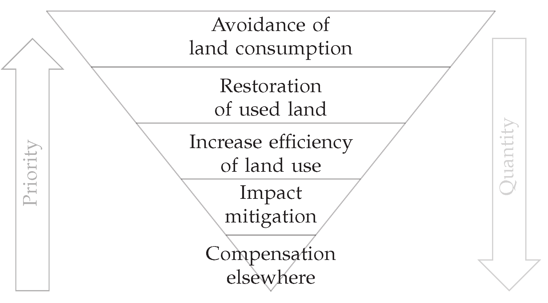
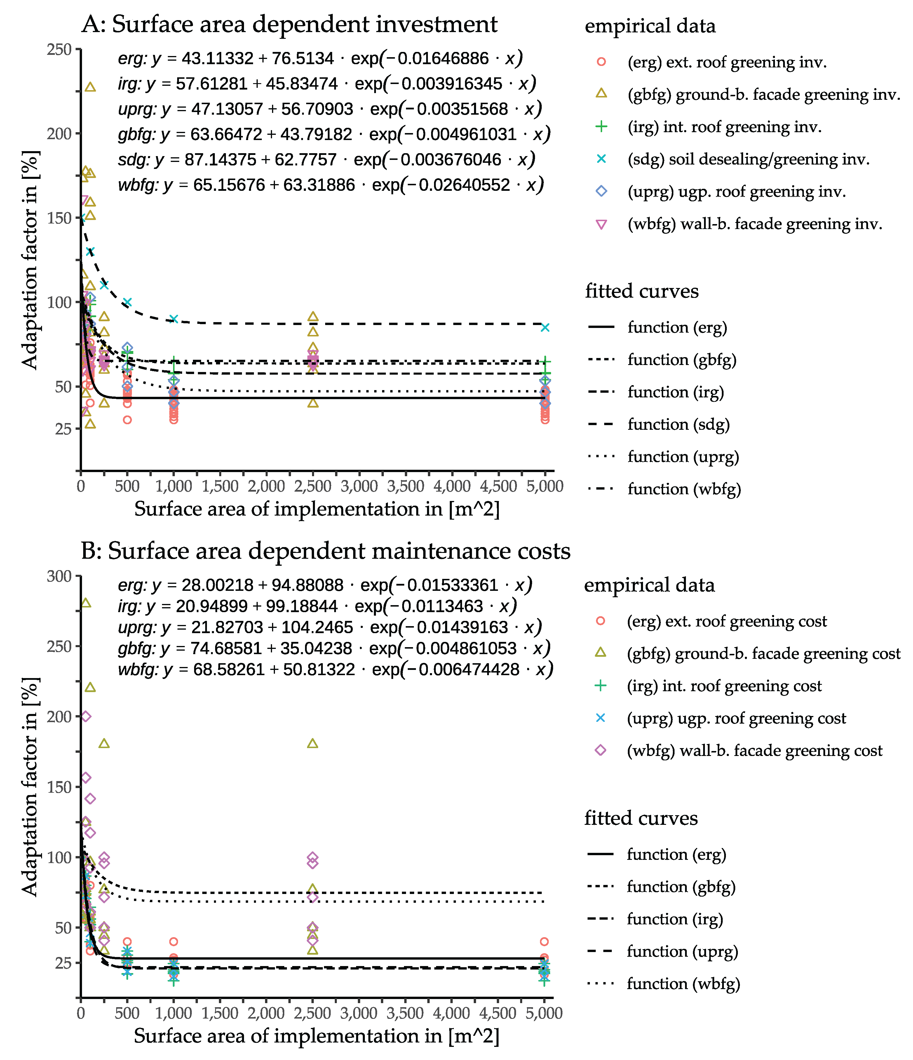
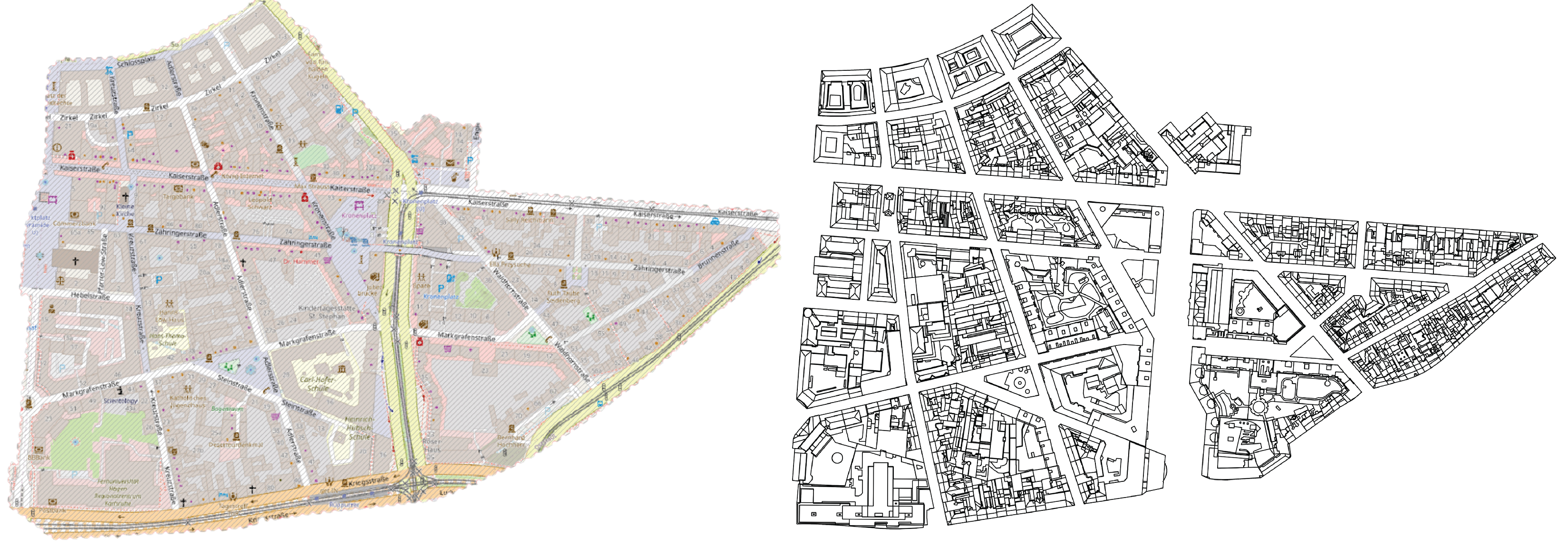
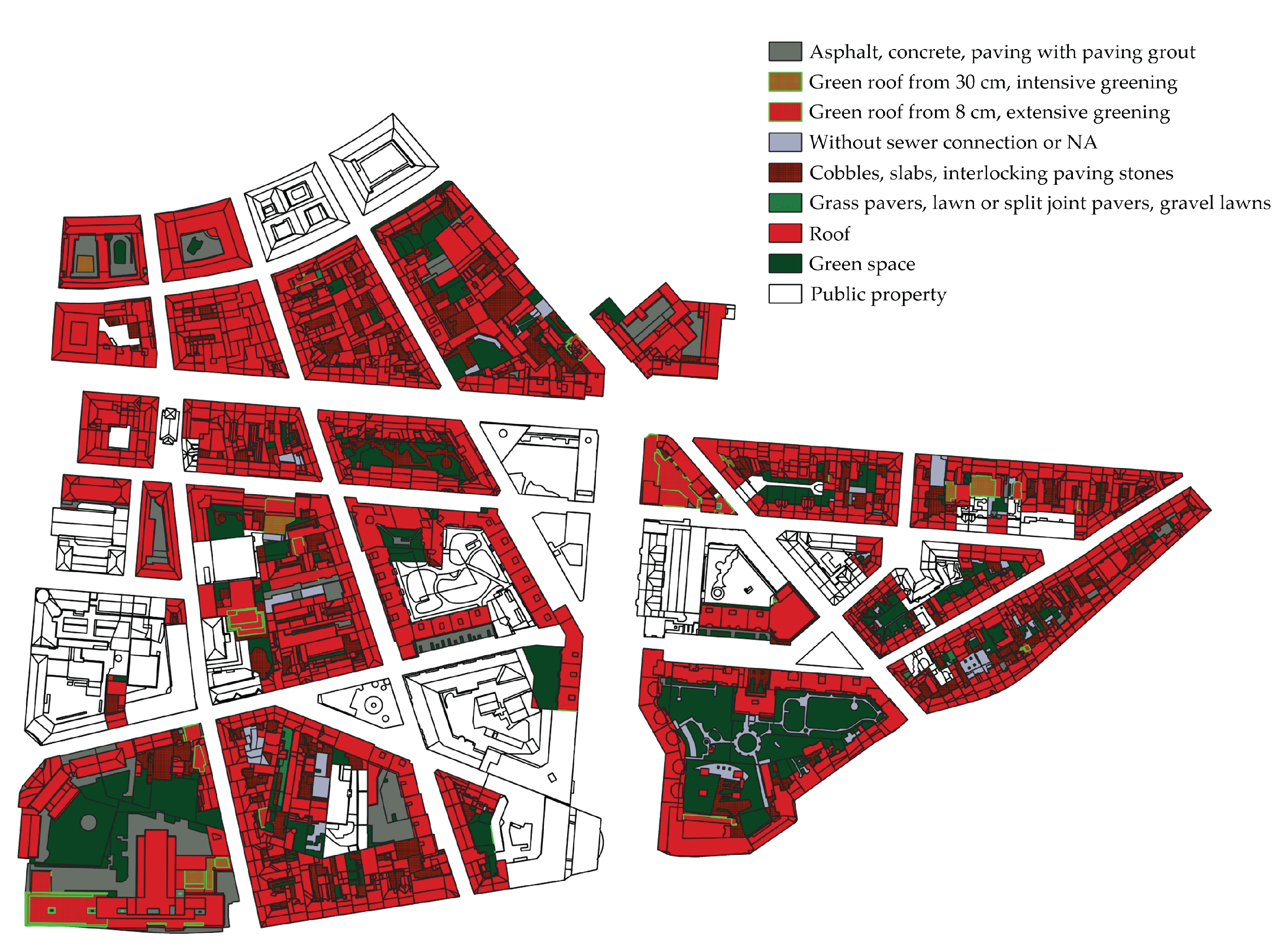
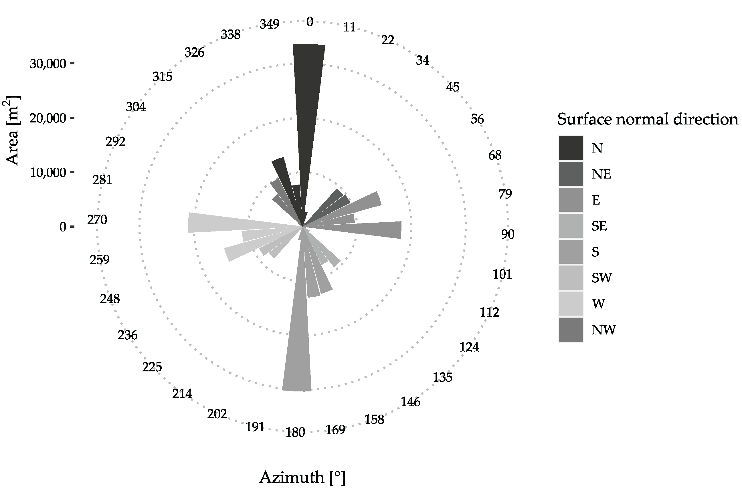
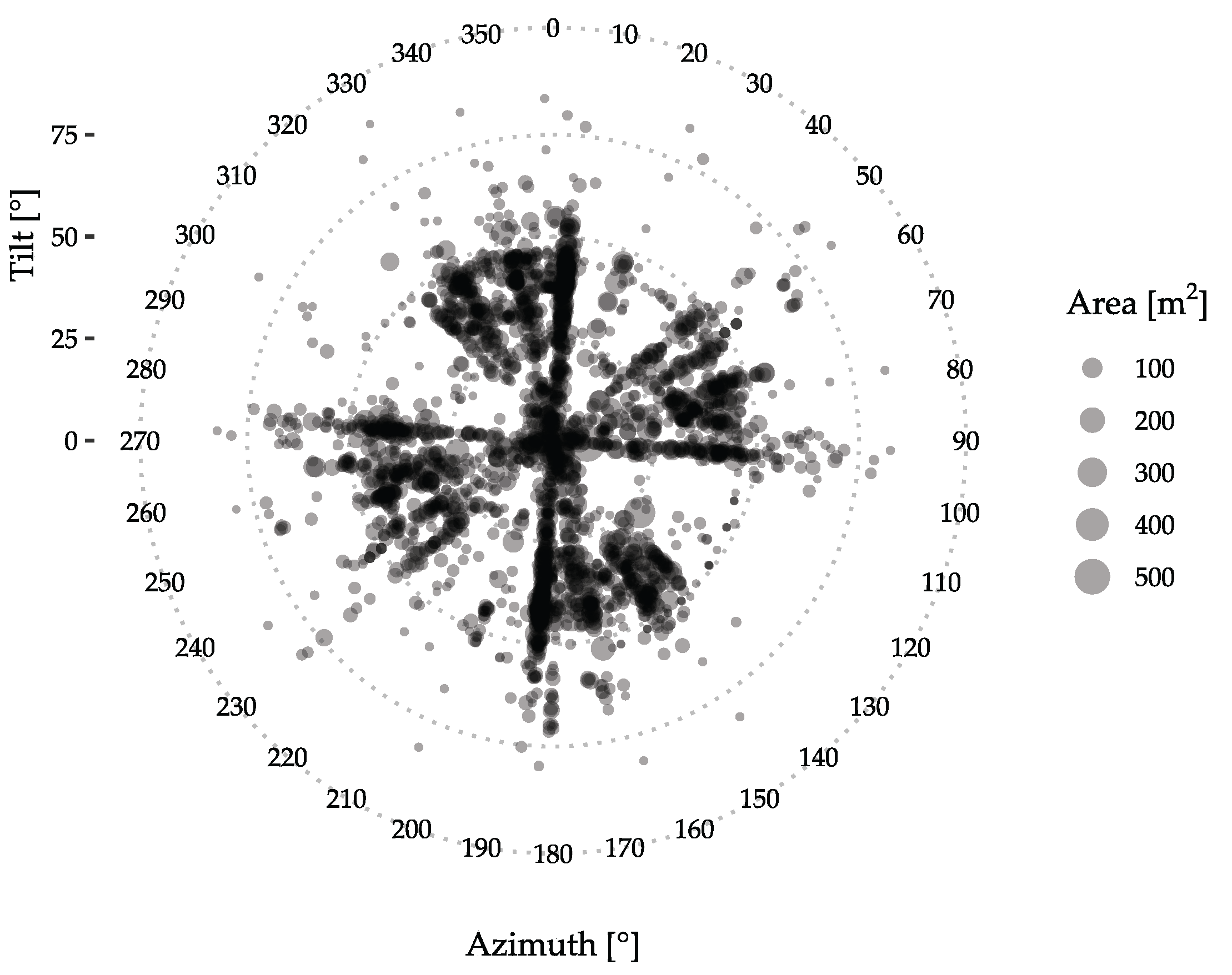
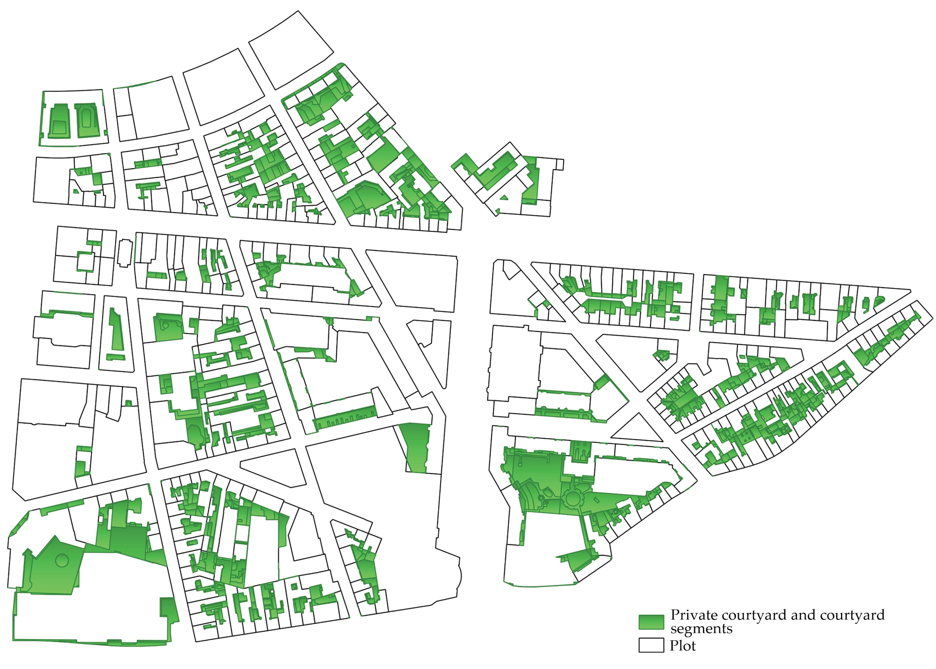
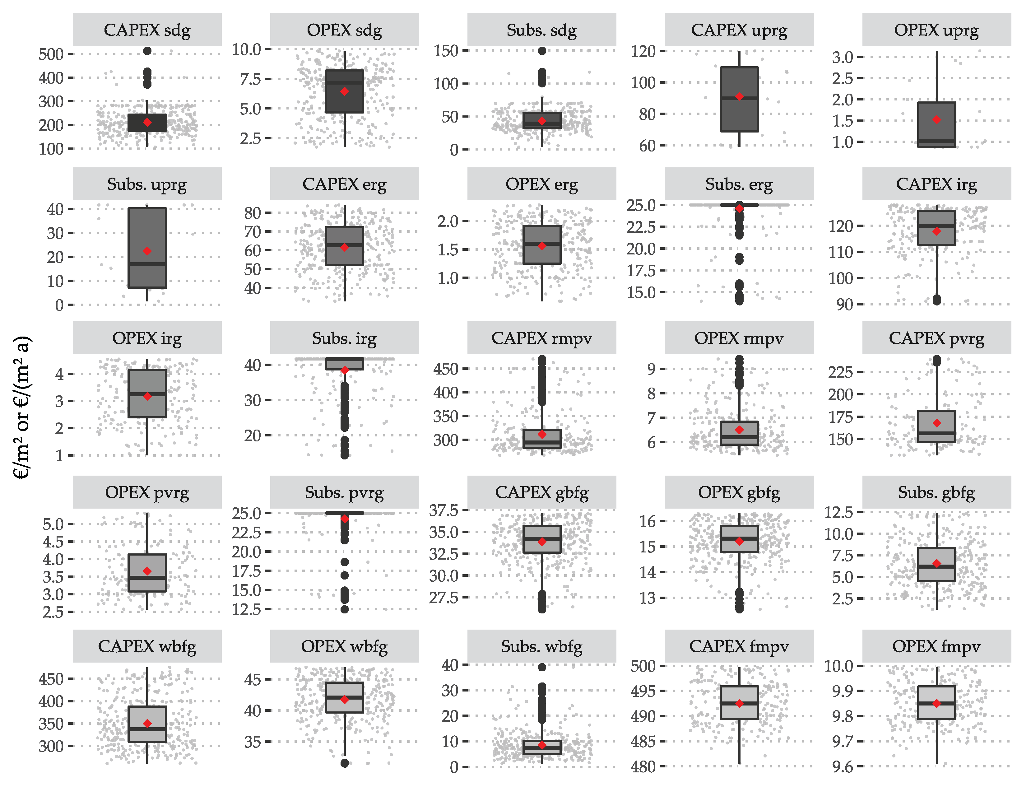
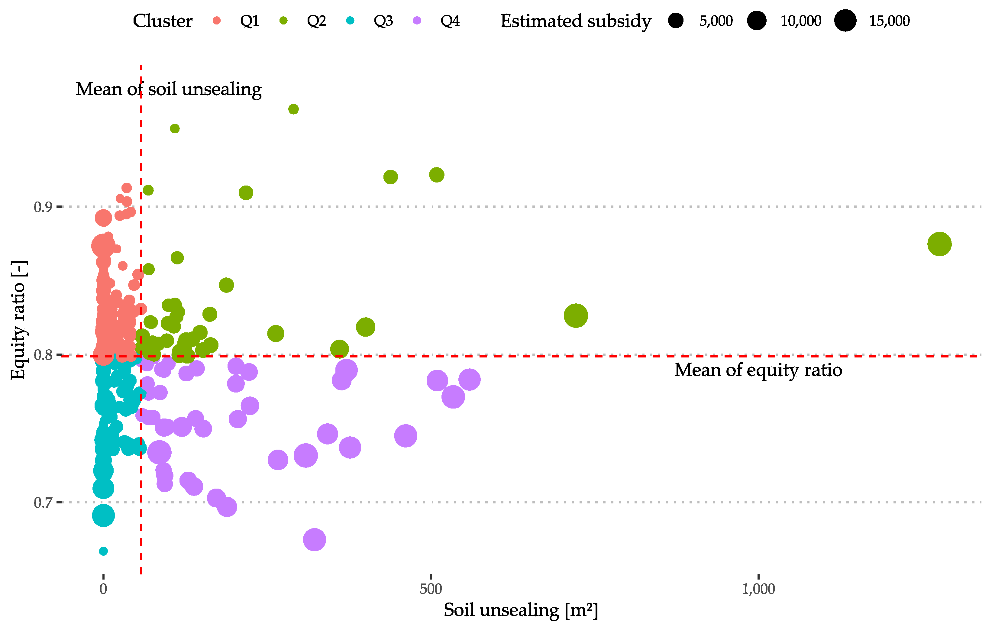
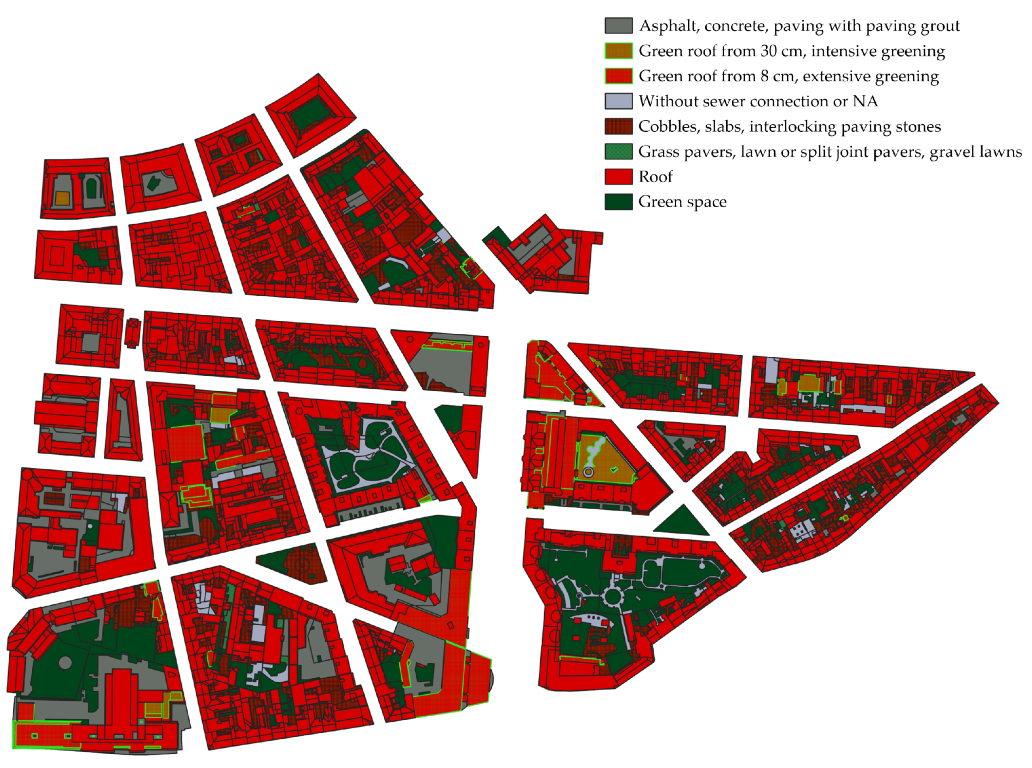
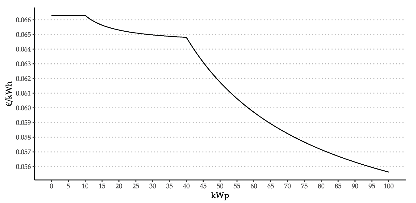
Table 1.
Minimal data inputs, case study data sources, and descriptions.
| Data Set | Brief Description or Meta Data Source | Source |
|---|---|---|
| Buildings and infrastructure (B) | Cadastral building and infrastructure footprints i with building use-type, (sub-)surface classification, name, address, ID information and other. | [79] |
| 3D LOD2 CityGML () | Geodata of solids and multi-surface building representations with standardised roof types. High position accuracy ii and object-IDs allow one to join and intersect with other data. | [79] |
| Land parcel (L) | Cadastral land parcels with address, ID information. | [79] |
| Namares survey (N) | Building survey for building archetype classification and individual building units/apartments count. | self-provided |
| Ownership (O) | Geodata of land parcels with public/municipal ownership. | [79] |
| Precipitation (P) | Local and long-term data on precipitation (annual and monthly). | [80] |
| Preservation and conservation interest () | Status regarding preservation, conservation, monument or other historic interest. | [81,82] |
| Solar irradiation () | Local statistical long-term data on solar irradiation, heating degree days and temperatures (annual and monthly). | [83] |
| Surface material () | Geodata on surface sealing and materials classification in high resolution (runoff water charge data iii). | [79] |
| Zoning (Z) | Aggregation layers for generating aggregated results. | self-provided |
i The cadastral data’s accuracy is below 3 cm for border points. ii The representations are based on the cadastral
building and infrastructure footprints i and light detection and ranging (Lidar). The accuracy of the LOD2 data
for height information is between 20 and 30 cm, 10 cm for the other dimensions. iii The polygon data is based on
cadastral building and infrastructure footprints i and measurements [84].
Table 2.
Spatial properties and identifiers of .
| Property | Value Description | Type iv | Source |
|---|---|---|---|
| IDs | Identifiers | ||
| Urban surface element ID () | Unique primary analysis unit/element ID | Integer | |
| Zoning ID () | Unique aggregation and statistical unit ID | Integer | |
| Land parcel ID () | Unique land lot or plot or parcel ID | Integer | |
| Building address () | Fixed format postal address | String | |
| Building ID () | Unique building ID | Integer | |
| Building element ID () | Unique identifiers for roof, facade, footprint elements | Integer | |
| Preservation/conservation ID () | Unique ID | Integer | |
| Surface material ID () | Unique identifiers for roof and sealed soil surfaces | Integer | |
| Geometries | Spatial data type | ||
| Urban surface element () | Polygon, multipolygon | Geom | |
| Zoning () | Polygon, multipolygon | Geom | |
| Land parcel () | Multipolygon | Geom | |
| Building () | Polyhedral surface | Geom | |
| Building element () | Polyhedral surface, polygon | Geom | |
| Preservation/conservation () | Point, line, polygon | Geom | |
| Surface material () | Multipolygon | Geom |
iv Geom: Geometry.
Table 3.
Non-spatial properties of .
| Property | Value Description | Type | Source |
|---|---|---|---|
| Parcel features | Non-spatial data type | ||
| Cistern () | States the presence of a rainwater cistern | Boolean | |
| Building features | Non-spatial data type | ||
| Building typology class () | 50 Episcope/Tabula residential building archetypes and more than 230 use-types (use-types according to ALKIS® classification) | String | |
| Superstructure volume () | Enclosed volume by the building envelope | Double | |
| Apartments/units () | Number of units in the building | Integer | |
| Building passage () | Special feature which is not part of the 3D LOD2 model | Boolean | |
| Arcade () | Special feature which is not part of the 3D LOD2 model | Boolean | |
| Cantilever or recessing facade () | Special feature which is not part of the 3D LOD2 model | Boolean | |
| Element features | Non-spatial data type | ||
| Surface type () | Surface type typology | String | |
| Surface cover type () | Surface cover typology derived from (Table 4) | String | |
| Orientation () | Surface normal which provides the azimuth | Double | |
| Tilt () | Surface tilt; Slope/pitch of a roof | Double | |
| Volume () | Element volume based on assumed thickness or material | Long | |
| Area () | Element area | Long | |
| Perimeter () | Element perimeter | Long | |
| x,y,z dimensions () | Point or vector information and length | Points | |
| Solar irradiation () | Annual and monthly azimuth and inclination dependent solar irradiation/global horizontal irradiation with | Long | |
| Precipitation () | Annual and monthly long-term precipitation with | Long | |
| Relative location to ground () | Elements position with regard to whether adjacent to the ground | Boolean | |
| Relative location to neighbouring features () | Elements position with regard to whether adjacent to other features, e.g., for party walls | Boolean | |
| Shape index () | Ratio of perimeter and area for element shape description and artefact detection | Double |
Table 4.
Surface cover types () of the initial state and surface material relations.
| Surface Cover Type | Surface Material Material |
|---|---|
| Impervious 1 () | Asphalt, concrete, paving with joint grouting |
| Impervious 2 () | Paving, slabs, interlocking stones |
| Impervious 3 () | Grass paving |
| Pervious () | Soil/urban green |
| Solid 1 () | Solid walls |
| Solid 2 () | Solid roofs |
| Extensive green () | Extensive roof greening <30 cm substrate thickness |
| Intensive green () | Intensive roof greening >30 cm substrate thickness |
Table 5.
Surface element selection for the technical potential assessment of measures .
| Measure (t) | Element Selection () v | Measure (t) | Element Selection () v |
|---|---|---|---|
 Extensive roof greening () Extensive roof greening () |  Intensive roof greening () Intensive roof greening () | ||
 Underground parking roof greening () Underground parking roof greening () |  Roof mounted photovoltaics () Roof mounted photovoltaics () | ∨ | |
 Photovoltaics and roof greening () Photovoltaics and roof greening () |  Ground-based facade greening () Ground-based facade greening () | ||
 Wall-based facade greening () Wall-based facade greening () |  Facade mounted photovoltaics () Facade mounted photovoltaics () | ||
 Soil desealing/ greening () Soil desealing/ greening () | |||
Table 6.
Technical potential input parameter for surface type (s) and measure (t) scope of implementation determination (based on [88,89,90,91]). The reduction factors account for obstruction (), shadowing (), utilisation (), pv (), efficiency (), and performance ratio ().
| Parameter () | vi | ||||||||
|---|---|---|---|---|---|---|---|---|---|
| vii | |||||||||
vi pitched roof, flat roof. vii vegetation, PV.
Table 7.
Input data for the economical assessment. Data were based on [37,84,92,93,94,95,96,97,98]. : CAPEX; : OPEX; : rates specific for a particular implementation size; : fixed part; : variable part; : electricity; : maintenance; : fees and charges for services; : self-consumption; : compensation for electricity fed into the grid.
| Parameter | Value | Parameter | Value |
|---|---|---|---|
Table 8.
Assessment indicators , units, and the respective parameters for the considered measures. Values are rounded and represent defaults and literature values.
Table 8.
Assessment indicators , units, and the respective parameters for the considered measures. Values are rounded and represent defaults and literature values.
| Parameter | Unit | viii | ix | x | |||||
|---|---|---|---|---|---|---|---|---|---|
| − | |||||||||
| xi | − | 1 | − | − | − | ||||
| xi | − | − | − | − | |||||
| xii | − | 0 | 0 | − | − | − | 0 | ||
| - xiii | 391 | 506 | 547 | 138 | 500 | 300 | 0 | ||
| xiv | 12 | 12 | 13 | ||||||
| 0 | 0 | 0 | xv | 0 | 0 | xv | xvi | ||
| xvii | 0 | xviii | xv,xvi | 0 | |||||
| xiv | 0 | 0 | xix | ||||||
| xx | 0 xv | 0 xv | |||||||
| xx | xv | xv | } | ||||||
| xx | 0 xv | 0 xv | |||||||
| xx | xv | xv | |||||||
| − | 1 | 1 | 1 | 1 | − | − | − | ||
| xxi | pt | 4 | 5 | 6 | 1 | 4 | 4 | 1 |
viii Short grass and herbaceous plants (1:1). ix Short grass, herbaceous plants and deciduous trees (2:1:1). x Configuration of porous plaster, green pavers (1:1 short grass, impervious) and domestic garden (1:1:1 short grass, herbaceous plants and deciduous trees). xi [103]. xii Based on [84]. xiii Based on [102]. xiv [37]. xv Per kWh and based on [104,105]. xvi Estimation based on [100] oak 0–20 years with 1000 trees per ha. xvii [106] xviii [107]. xix [108]. xx Based on [101]. xxi [77].
Table 9.
Initial state surface parameters. Values are rounded and represent defaults and literature values.
Table 9.
Initial state surface parameters. Values are rounded and represent defaults and literature values.
| Parameter | Unit | p | |||||||
|---|---|---|---|---|---|---|---|---|---|
| − | |||||||||
| xi | − | 1 | − | 1 | |||||
| xi | − | − | |||||||
| xii | − | 1 | 0 | − | 1 | 0 | |||
| - xiii | 147 | 147 | 277 | 490 | 0 | 138 | 391 | 580 | |
| xiv | 13 | 13 | |||||||
| 0 | 0 | 0 | xvi | 0 | 0 | 0 | 0 | ||
| xvii | 0 | 0 | 0 | 0 | |||||
| xiv | 0 | 0 | 2 | 0 | 0 | ||||
| xx | 0 | 0 | 0 | 0 | |||||
| xx | 0 | 0 | 0 | 0 | |||||
| xx | 0 | 0 | 0 | 0 | |||||
| xx | |||||||||
| - | 1 | 1 | 1 | 0 | − | 1 | 1 | 1 | |
| xxi | - | 1 | 1 | 2 | 6 | 1 | 1 | 4 | 5 |
The explanations of superscript are the same as Table 8.
Table 10.
Surface inventory of surfaces of private ownership in the case study (Section 3.5). Values are rounded and represent aggregates on plot (pl.) level. Sub.: substructure.
Table 10.
Surface inventory of surfaces of private ownership in the case study (Section 3.5). Values are rounded and represent aggregates on plot (pl.) level. Sub.: substructure.
| Type of Surface (s) | Count of Plots | Total Area [h] | Median [m] | Mean [m] | Total Vegetated [ha] | Count of Vegetated pl. | Median [m] | Mean [m] | % of Total Area |
|---|---|---|---|---|---|---|---|---|---|
| Ground xxii | 372 | xxiii | 304 | 524 | − | − | − | ||
| Courtyards | 330 | 87 | 165 | 166 | |||||
| Sub. roof | 43 | 42 | 364 | 14 | 254 | 493 | |||
| Roof | 350 | 177 | 237 | − | − | − | |||
| Flat | 264 | 65 | 203 | 23 | 144 | 358 | |||
| Tilted | 320 | 204 | 277 | 14 | 65 | 113 | |||
| Wall | 350 | 1062 | 1466 | xxiv | − | − | − | − | |
| Facade | 350 | 528 | 810 | xxiv | − | − | − | − | |
| Party wall | 350 | 452 | 605 | xxiv | − | − | − | − | |
| Other | 135 | 73 | 131 | xxiv | − | − | − | − | |
| Total | xxv | xxiv |
xxii Total ground-level which includes sub- and superstructures. xxiii Represents the footprint area of all sub-,
superstructure and soil surfaces. xxiv No detailed surface cover type available. Random onsite inspections revealed
some vegetation but no widespread vegetation on facades could be concluded. xxv Without vertical surfaces.
Table 11.
Potentials in the case study area and assessment of effects. The values represent aggregates for each measure and the effect/change () from the initial state for the potential area. The column Initial represents the initial state in absolute values. All values are rounded. pp: percentage point.
| Category | xxvi | |||||||||
|---|---|---|---|---|---|---|---|---|---|---|
| Effective are xxvii [] | 4 | xxviii | 2 xxix | − | ||||||
| Selectable area xxx | xxxi | |||||||||
| Albedo [-] | 0.03 | 0.01 | −0.03 | −0.03 | −0.01 | −0.03 | −0.02 | 0 | 0 | 0.211 |
| Runoff peak [pp] | −40 | −39 | −24 | −46 | 0 | −29 | 0 | 0 | 0 | 84 |
| Runoff avg [pp] | −37 | −37 | −30 | −47 | 1 | −35 | 0 | 0 | 0 | 69.6 |
| Soil sealing [pp] | −35 | 0 | 0 | 0 | 0 | 0 | 0 | 0 | 0 | 89 |
| CAPEX [m€] | 27 | − | ||||||||
| OPEX | − | |||||||||
| Savings | 2 | 9 | 11 | 242 | 148 | 0 | 0 | 194 | − | |
| Earnings | 0 | 0 | 0 | 0 | 107 | 63 | 0 | 0 | 85 | − |
| Local subsidies [m€] | 0 | 0 | − | |||||||
| Green waste | 37 | 4 | 0 | 2 | 0 | |||||
| Evapotrans. | 0 | 0 | ||||||||
| Value of evapotrans. | 2 | 0 | 10 | 0 | ||||||
| [t] | 19 | 32 | 0 | 102 | 103 | 0 | ||||
| 0 | 0 | 0 | 986 | 585 | 0 | 0 | 790 | − | ||
| Biodiversity [k n] | 220 | 90 | 400 | 250 | 0 | 200 | 1100 | 860 | 0 | 661 |
| 93 | 59 | 0 | 48 | 304 | 200 | 0 | ||||
| 26 | 18 | 86 | 56 | 24 | ||||||
| 180 | 114 | 0 | 92 | 610 | 385 | 0 | ||||
| 41 | 27 | 0 | 21 | 175 | 87 | 0 | ||||
| [pt] | 85,517 | 39,690 | 120,263 | 88,936 | 0 | 61,724 | 253,069 | 255,234 | 0 | 620,513 |
xxvi All values are absolute and summarise ground, facade and roof surfaces. It should be noted that the facade greening status is unknown. xxvii Area of potential. xxviii Area need for PV panels. xxix Area need for greening with PV panels. Thus, greening area ≠ PV panel area. xxx Element area after selection σφ(E). xxxi Union of selectable areas.
Table 12.
Local subsidy program analysis for soil unsealing by the measure .
| Quadrants | Below Average Soil Unsealing | Above Average Soil Unsealing |
|---|---|---|
| Above average equity ratio | Q1: subsidies for () | Q2: subsidies for () |
| Below average equity ratio | Q3: subsidies for () | Q4: subsidies for () |
Publisher’s Note: MDPI stays neutral with regard to jurisdictional claims in published maps and institutional affiliations. |
© 2022 by the authors. Licensee MDPI, Basel, Switzerland. This article is an open access article distributed under the terms and conditions of the Creative Commons Attribution (CC BY) license (https://creativecommons.org/licenses/by/4.0/).
Share and Cite
MDPI and ACS Style
Naber, E.; Volk, R.; Mörmann, K.; Boehnke, D.; Lützkendorf, T.; Schultmann, F. Namares—A Surface Inventory and Intervention Assessment Model for Urban Resource Management. Sustainability 2022, 14, 8485. https://doi.org/10.3390/su14148485
AMA Style
Naber E, Volk R, Mörmann K, Boehnke D, Lützkendorf T, Schultmann F. Namares—A Surface Inventory and Intervention Assessment Model for Urban Resource Management. Sustainability. 2022; 14(14):8485. https://doi.org/10.3390/su14148485
Chicago/Turabian StyleNaber, Elias, Rebekka Volk, Kai Mörmann, Denise Boehnke, Thomas Lützkendorf, and Frank Schultmann. 2022. "Namares—A Surface Inventory and Intervention Assessment Model for Urban Resource Management" Sustainability 14, no. 14: 8485. https://doi.org/10.3390/su14148485
Note that from the first issue of 2016, this journal uses article numbers instead of page numbers. See further details here.