Article

Geo-Crowdsourced Sound Level Data in Support of the Community Facilities Planning. A Methodological Proposal

by
Gabriella Graziuso
1,
Simona Mancini
2,
Antonella Bianca Francavilla
1,
Michele Grimaldi
1 and
Claudio Guarnaccia
1,*
1
Department of Civil Engineering, University of Salerno, 84084 Fisciano, Italy
2
Department of Information and Electric Engineering and Applied Mathematics, University of Salerno, 84084 Fisciano, Italy
*
Author to whom correspondence should be addressed.
Sustainability 2021, 13(10), 5486; https://doi.org/10.3390/su13105486
Submission received: 2 April 2021 / Revised: 30 April 2021 / Accepted: 10 May 2021 / Published: 14 May 2021

Abstract

:
To reduce environmental noise pollution and to safeguard people’s well-being, it is urgently necessary to move towards sustainable urban development and reconcile demographic and economic growth with the protection and restoration of the environment and the improvement of the quality of human lives. This challenge should be a concern to policymakers, who must issue regulations and define the appropriate actions for noise monitoring and management, and citizens, who must be sensitive to the problem and act accordingly. Starting from an analysis of several crowdsourcing noise data collection tools, this paper focuses on the definition of a methodology for data analysis and mapping. The sound sensing system, indeed, enables mobile devices, such as smartphones and tablets, to become a low-cost data collection for monitoring environmental noise. For this study, the “NoiseCapture” application developed in France by CNRS and IFSTTAR has been utilized. The measurements acquired in 2018 and 2019 at the Fisciano Campus at the University of Salerno were integrated with the kernel density estimation. This is a spatial analysis technique that allows for the elaboration of sound level density maps, defined spatially and temporally. These maps, overlaid on a campus facilities map, can become tools to support the appropriate mitigation actions.

1. Introduction

Population growth, urbanization, and socio-economic evolution have produced an increase in mankind’s industrial, commercial, transport-related, and recreational activities. These cause a worsening of sound pollution in urban areas [1] and its auditory and non-auditory effects on human health, such as annoyance, sleep bothers, hypertension, cardiovascular disease, and impaired cognitive performance in schoolchildren [2]. Currently, the European Environment Agency (EEA) estimates that almost 20% of the population in Europe is exposed to harmful noise levels daily [3].
Consequently, noise impact is a growing concern among both the general public and authorities. In 1999, to protect human health, the World Health Organization (WHO) published some recommendations on noise level values [4], which were updated for some of the sources, such as transportation (road traffic, railway, and aircraft), wind turbine, and leisure noise [5] in 2018. Moreover, many regulations have been issued in the last decades to select the acoustic indicators, define people’s exposure, and propose noise control procedures to reduce and prevent noise pollution. The European Union (EU), for instance, enacted a directive on environmental noise in 2002, inviting the EU member states to produce strategic noise maps and action plans [6]. Those maps must be produced concerning sound emission calculations and mathematical models for the propagation law of sound, using standard or advanced methods, or with the aid of a measurement campaign [7,8,9,10,11,12,13]. However, both these approaches have some limitations [14]. The emission models, indeed, often represent a simplification of the reality, referring, for example, to traffic sound sources without considering other sources or people’s perception of noise and making other approximations about the traffic flow, the weather conditions, the morphology, and the ground type [15,16]. Moreover, a measurement campaign in an urban area requires a considerable number of points of measurements [14], based on expensive equipment dedicated to noise collection, that must consider the phenomenon dynamically, making this technique almost unsustainable.
Recently, another approach that involves people in the data acquisition is becoming increasingly popular in the research field [17]. Each citizen can easily contribute to environmental noise data collection with the use of smartphones and tablets [18]. These devices, combined with GPS tracking, allow the display of the results in interactive maps and the generation of noise maps in a GIS-based model. Consequently, participatory sensing could be considered a low-cost alternative to large-scale and costly infrastructure sensing based on sensor networks [19]. Despite less adequate accuracy, this approach could lead to the production of more realistic noise maps [20], integrating all the involved sound sources and their temporal dynamics.
These noise maps become essential to promote urban planning procedures according to sustainable development standards [21], as defined in the 11th Goal of the 2030 Agenda [22]. Since public and private community facilities in an urban area must be planned according to their economic, social, and environmental impacts, their location must be defined according to several criteria [23]. Among others, total noise pollution is a feature that must be considered [24]: for instance, some noise-emitting facilities need to be placed far away from sensitive buildings, such as hospitals and schools. Moreover, another consideration can be outlined: community facilities can generate noise, but also, they can be affected by noise [25].
Starting from these considerations, this paper aims to deepen understanding of some aspects related to environmental noise mapping and its relationship with the community facilities. The first focus is on highlighting the potential of crowdsourcing data collection tools for the acquisition of voluntary data on sound pressure levels. The second aspect concentrates on the generation of sound density maps in a geographic information system (GIS) to comprehend the sound distribution, both spatially and temporally. Finally, the third point is the generation of a solution matrix, derived from the analysis of the relationship between noise and community facilities. Specifically, after the description of the tools used for the data acquisition and their elaboration, the definition of a methodology for noise analysis and generation of acoustic concentration maps, based on the kernel density estimation, is described in Section 3. The methodology becomes a tool for supporting urban planning decisions, because it integrates noise density maps with public facilities maps. In Section 4, the results deriving from the application of the methodology to the Fisciano Campus of the University of Salerno (Italy) are described, and finally, Section 5 contains the main conclusions of this research.

2. Data Collecting and Mapping

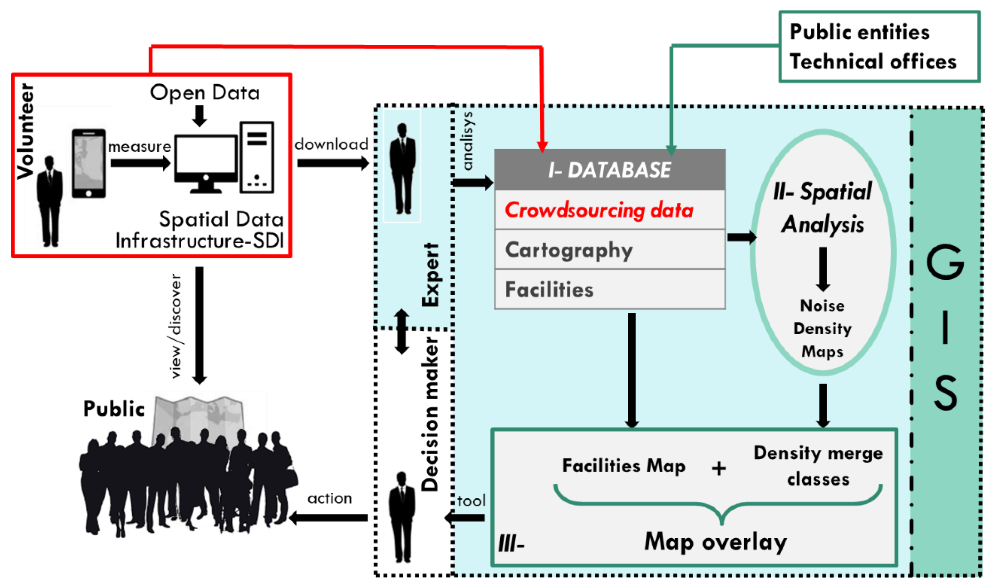
2.1. Participatory Tools for Environmental Noise Assessment

The increasingly widespread tendency to involve citizens in data collection and the extremely large number of people equipped with a mobile device (3.8 billion users worldwide is forecasted in 2021 [26]) have led to the awareness that the use of smartphones is potentially a relevant solution to realize a large-scale environmental noise evaluation. Moreover, the continuous improvement of smartphone features and the creation of appropriate applications allow the acquisition of noise data easily and the creation of noise observation networks, spatially and temporally. This approach does not represent a novelty and, in line with citizens’ science, volunteers taking part in the scientific research have been already found in many disciplines, such as health research [27] or environmental monitoring [28]. Regarding environmental issues, public involvement has been also acknowledged by the European Directive 2003/35/EC [29].
Currently, numerous platforms and tools for environmental noise study utilize the approach of crowdsourcing data collection. In [17,30], the authors show the features of several applications aimed at noise control, such as Laermometer, 2Loud?, NoiseWatch, UbiSound, and NoiseTubePrime. Moreover, other applications and projects are: Noise-Tube project [31,32]; the WideNoise application, developed within EveryAware project [33]; NoiseSPY, which is part of the MobSens project, that integrates three other mobile phone applications dedicated to health, social, and air pollution sensing [34]; the NoizCrowd application, belonging to the BioMPE project [35]; SoundOfTheCity, Ear-phone, and MobGeoSen applications [36]; the NoiseMap application [37]; NoiseBattle and NoiseQuest prototypes, which are based on the open-source application NoiseDroid and collect noise data through gaming techniques [38,39]; the NoiseCapture application of the Noise-Planet project [40]; and the OpeNoise application developed by the Regional Agency for Environmental Protection of Piedmont in Italy [41]. Typically, these platforms are client–server systems that integrate a mobile application used by volunteers and a central server application.
The mobile application enables users to measure noise parameters everywhere and at any time. In many cases, the application is available for free for smartphone users, both iOS and Android models. Other aspects are related to the possibility that the applications can record and collect both perceptive and acoustic data and other contextual information that can be provided by users employing a tagging component with the upload of pictures or the reply to perceptive questionnaires. Finally, to preserve the volunteers’ privacy, the applications collect encrypted data [30,42,43]. Table 1 compares some applications in terms of their functionalities that give participants information on their level or community level of exposure, on health risk assessment, context awareness, and allow them to share their experience of exposure concerning their feelings about the sound. The table summarizes results presented in [17,30,36] and implements other applications. The first 6 rows and 5 columns in the table indicates respectively the apps and the features common to the three studies, and the stars mean that the features need future improvements.
The central server application is necessary for receiving and storing measured data, uploaded by volunteers automatically or manually and, only later, it will be possible to generate maps that show the geographical distribution of the measured parameters [32,44]. The described infrastructure is fully based on open-source tools and programming languages that perfectly comply with geographical standards and facilitate data exchanges toward a global centered hub [45].
The main steps of the data acquisition procedures are the initialization of the noise measurements, the upload of the collected data to a server application, and finally, the visualization on a geo-located noise map [42,46]. Moreover, these platforms are based on four levels of stakeholders:
  • the volunteer, who collects noise data with a smartphone and publishes it on the central server application, which can be considered a spatial data infrastructure (SDI);
  • the expert (geographer, acoustician, urban planner, and researchers), who can manage and understand the raw data, extracted from the SDI, and use them in several applications;
  • the decision maker, who can use the information as a support for land management decisions;
  • the public, who are represented by citizens who can use the visualization services to be aware of noise issues and understand the mitigation actions implemented by the decision maker for managing noise pollution.
The scientific community is debating the use of these applications as an alternative to the traditional measurement instrumentation [47] because the results are often affected by errors concerning both the sound levels and their localization. The mobile devices used for sound measurements and the professional instruments, such as sound level meters, are characterized by different microphone hardware, filters, and sound application programming interfaces for processing the measured data [48]. The measurement accuracy, indeed, is strictly connected with its purpose and the different features of mobile devices available in the market [49,50,51]. Generally, a specific treatment of the collected raw data, such as a post measurement cross-calibration procedure, is necessary to correct the smartphones’ microphone response. Sakagami et al. [49] examined the accuracy of acoustic measurements of both iOS and Android types, observing that it depends on the application, its calibration function, and the type of microphone. Additionally, the accuracy is continuously improving because the devices and the applications are often updated, and new versions appear frequently. Moreover, Murphy and King [52] reported that applications for noise measurement for the iOS platform are superior to those working on the Android platform, probably because of higher quality control, a better quality of microphones, and less variation in smartphone models. However, the Android models are more popular worldwide than the iOS ones. Another accuracy concerns the geo-localization of collected data due to the GPS data deviation (a typical precision is about 10–50 m) that can produce errors that allocate high noise levels to quiet environments [20].
Several works [33,50,53] demonstrate that, when the operations of measurement are coordinated properly, the acquired data can produce collective noise maps comparable to simulation-based maps. Despite the lower quality of acoustic measurements than the traditional methods, Guillaume et al. [17] discussed the relevance of the approach. Also, the accuracy of the results obtained in the acoustic field was studied by Aumond et al. [54] and Can et al. [55], who reported that using mobile devices to collect noise data is better than using the interpolation method to produce noise maps. Moreover, Grubeša et al. [56] concluded that smartphones could be used as instruments for creating, or even checking, final noise maps in an urban environment. Consequently, researchers’ interest in this approach is growing.
Since measurements are achieved completely freely, a further observation on this approach is that some areas and some periods are covered with a very high statistical representativeness, while others only gather a few (or no) measurements. Therefore, the production of a single aggregate noise map implies the introduction of a statistical component. Consequently, after the division of the surveyed area into smaller areas using a regular grid and the partition of the set of measurements over those areas based on their geographic coordinates, it is necessary to perform a statistical analysis per unit area which allows the generation of a map made of average values with coded colors on each pertaining area [46].

2.2. Participatory Tools for Environmental Noise Assessment

To overcome the problem of non-continuity between cells, techniques of spatial concentration, such as the function of the kernel density estimation (KDE), can be applied. The KDE belongs to the point pattern analysis, which is a family of spatial analysis techniques developed starting from the first principle of geography by Tobler [57]: “All things are related, but nearby things are more related than distant things”, and implemented by Gatrell et al. [58] in their studies on the spread of epidemics. Given a phenomenon, this kind of analysis studies the distribution of events throughout a region and, from sources of punctual vector data, there is a generation of grids that are classified according to associated numerical attributes [59].
The method is based on the density and, with regards to heterogeneous distributions of points, the focus shifts to the calculation of the local density. In particular, the density is estimated by counting the number of events in a region, said kernel, centered at the point where it is preferred to have the estimate. It is necessary, therefore, that each Li event is uniquely and spatially identified by the coordinates xi, yi. Accordingly, an event Li is a function of the position and its attributes. While the simple density function examines the number of events for each element of the regular grid that composes the R study region, the kernel density considers a movable surface in three dimensions, which weighs the events according to their distance from the point at which the intensity is estimated [60].
The density or intensity λ(L) of the distribution at the point L can be defined by the equation:
λ ( L ) = i = 1 n 1 τ 2 k ( L L i τ ) ,
where Li is the i-th event; k(L, Li, τ) is the kernel function, which weighs the events according to their distance from the point it is estimated; and τ is the bandwidth, i.e., the radius of the circle centered at L within which the events contribute to the estimate (Figure 1). The choice of the bandwidth affects greatly the resulting surface of estimated density. If the bandwidth is big, the kernel density is considerably closer to or coincides with the values of the simple density. If the bandwidth is rather small, the resulting surface will tend to catch single events with near-zero density for elements of the grid that are far from each event. The bandwidth must be evaluated according to the phenomenon, which must be analyzed and determined for subsequent adjustments [61].
Thanks to the integration of kernel density estimation in a GIS environment, it is possible to produce raster maps depending on the attributes associated with geometric primitives that are representative of the designed pattern [62,63]. These maps of concentration, which can be named “density maps”, contribute to understanding the distribution of the phenomenon in a region starting from the punctual measurements performed [64].

3. Materials and Methods

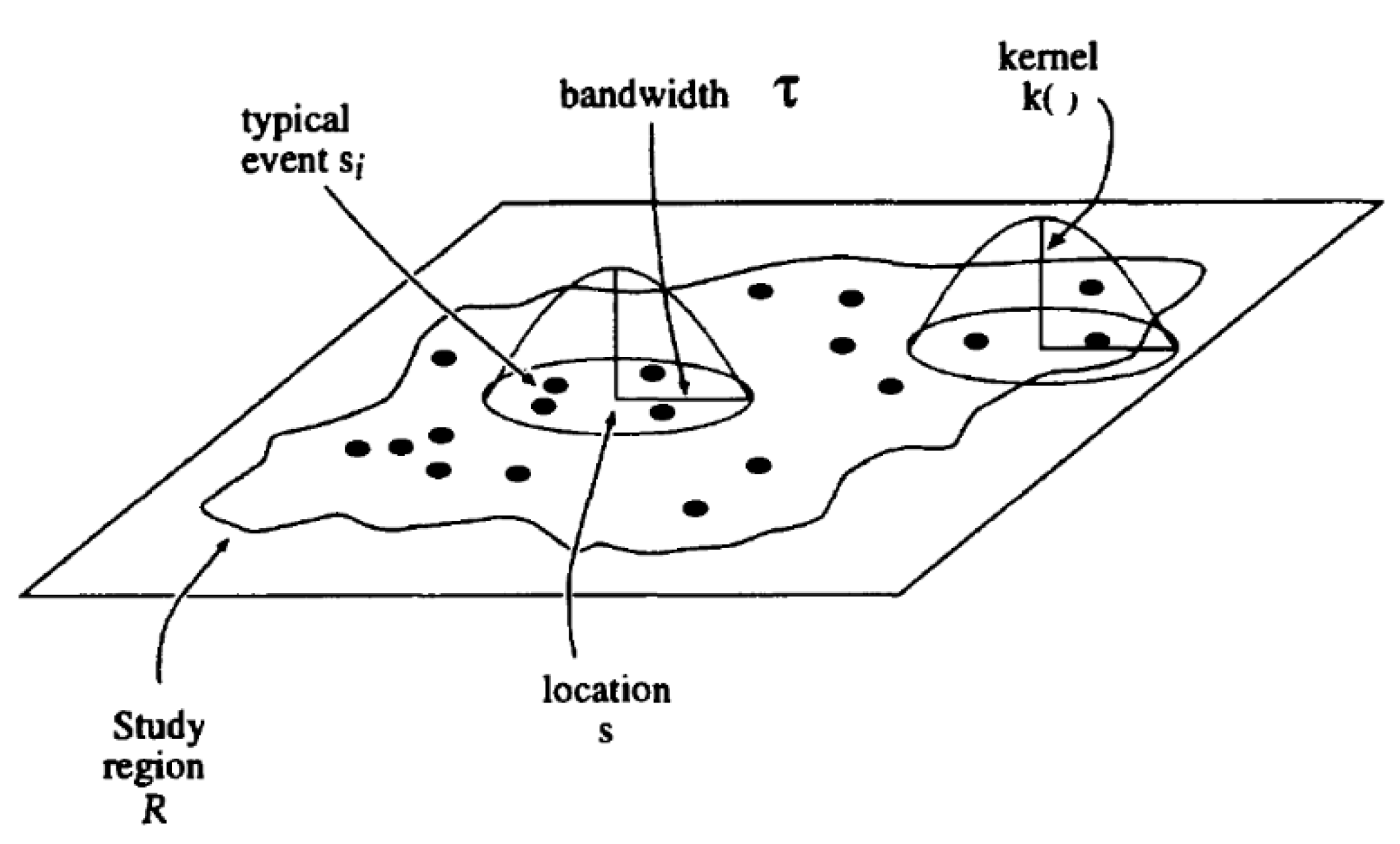
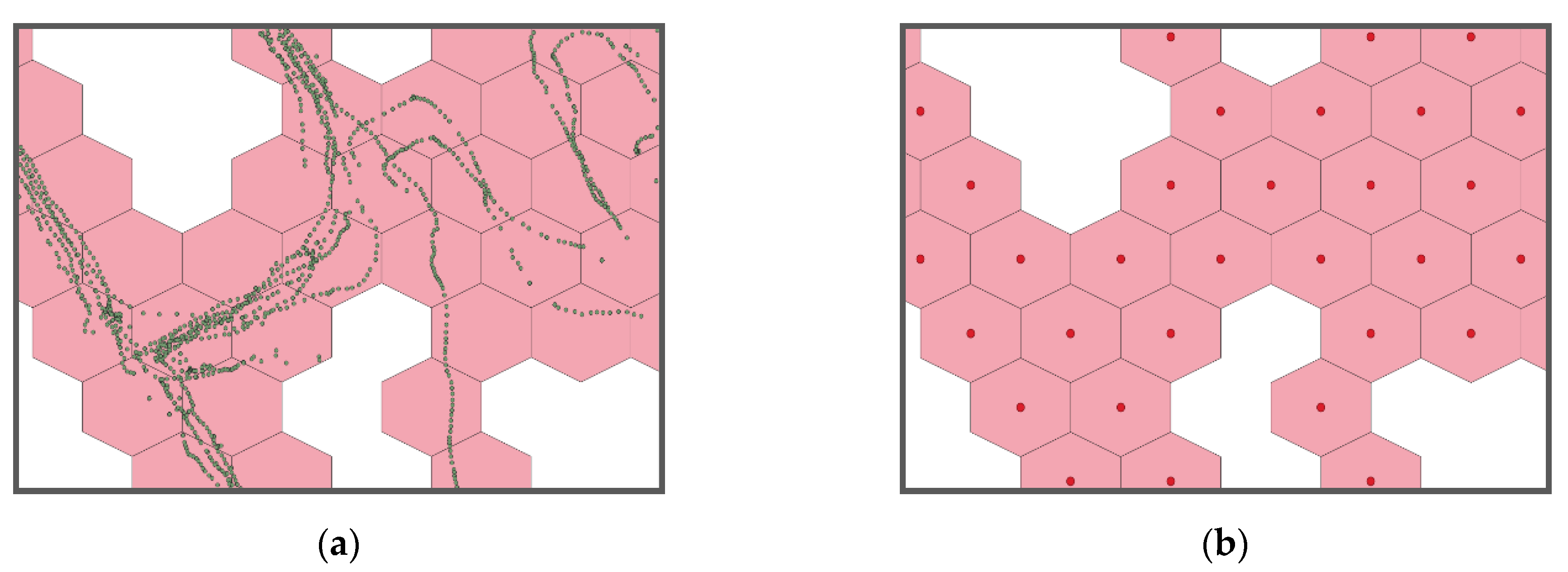
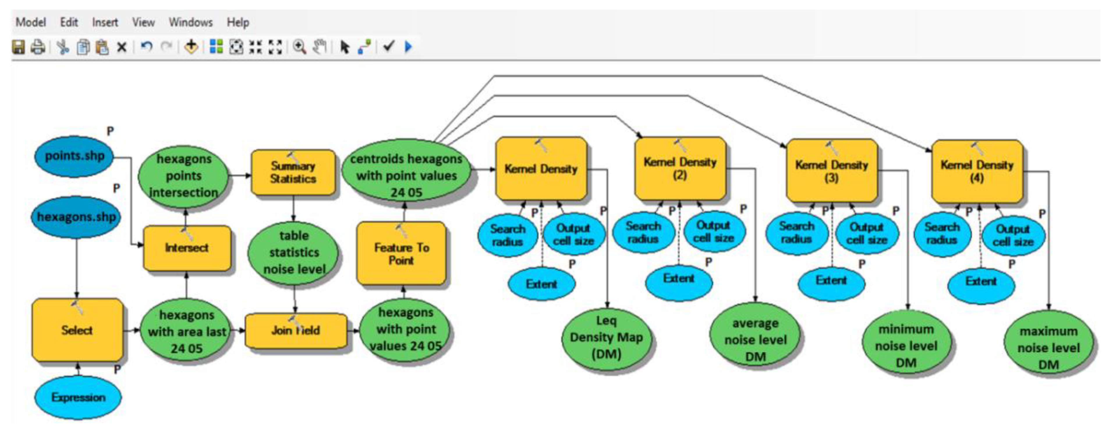
3.1. Methodology for Noise Analysis and Mapping
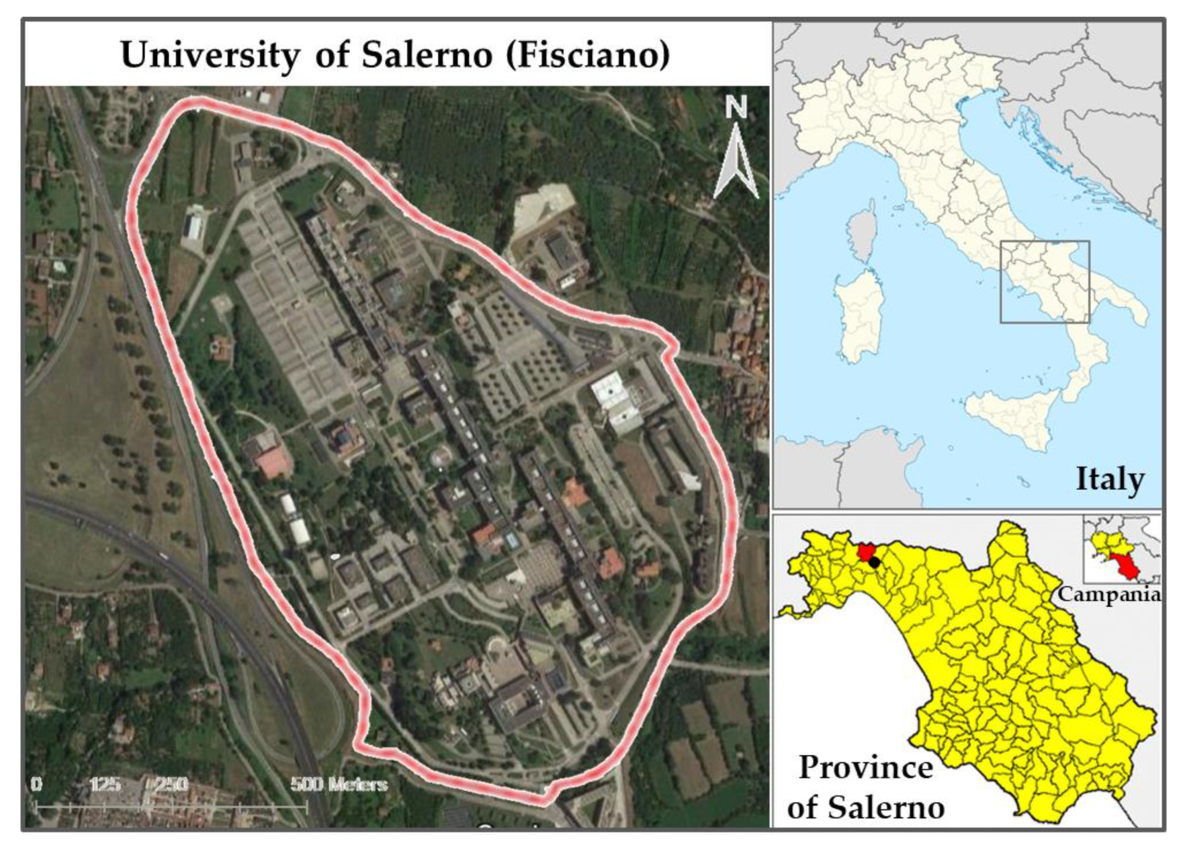
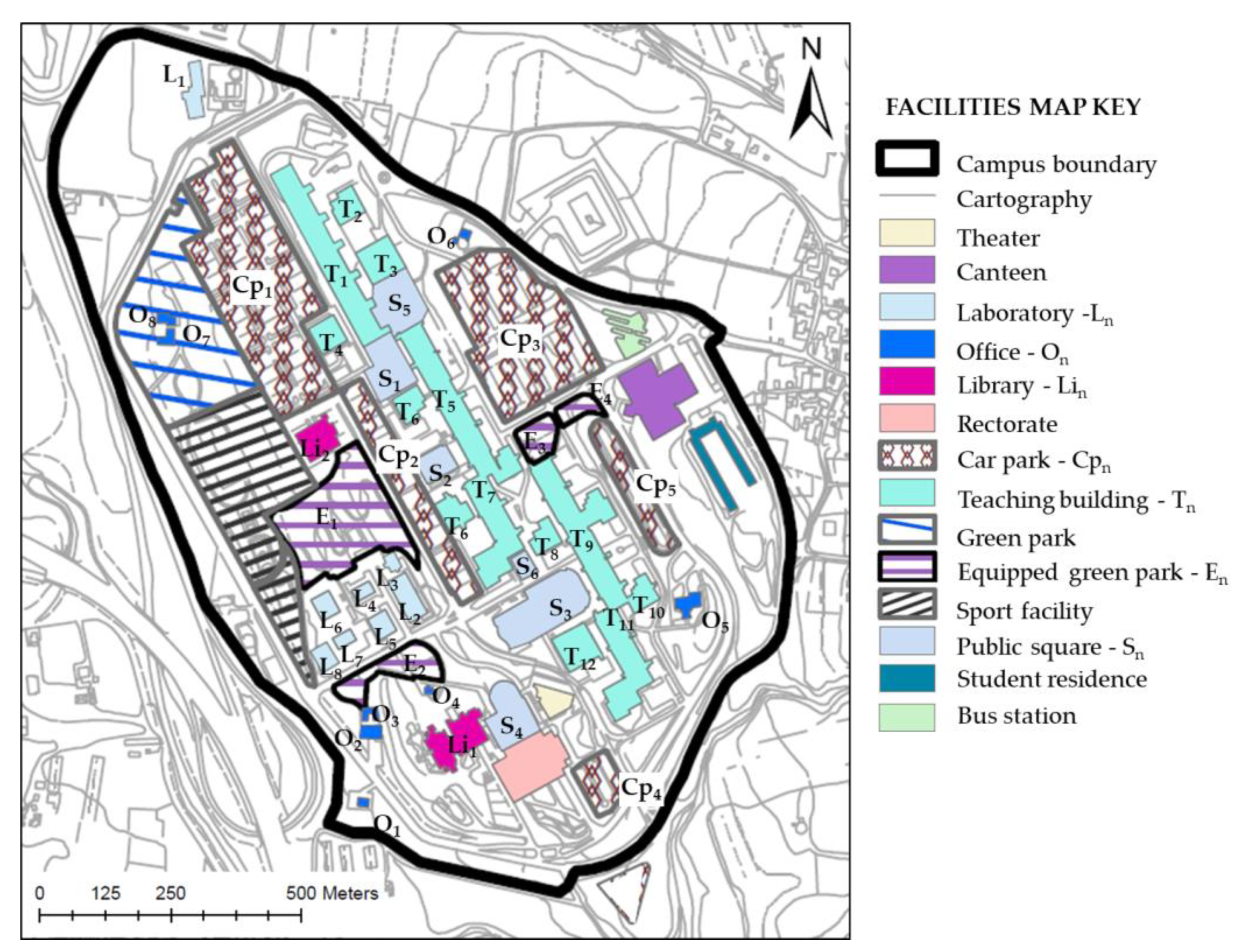
Starting from the organization of the participatory noise platform and the stakeholders involved, a methodology for data analysis and mapping is developed in this section. The proposal regards the experts who, with the data collected in crowdsourcing, can make further analysis. The whole process can be developed in a GIS environment and is organized into three phases (Figure 2).
First, the expert builds a database made of the crowdsourcing data, open data, and all the official information shared by other infrastructures, such as public bodies and technical offices.
The second phase performs a spatial analysis of the phenomenon. Since both acoustic and statistical indicators are computed for the whole duration of the measurement, it is possible to generate their density maps through the kernel density estimation function. These maps can be understood as sound and perceived effective maps of the study region. Additionally, a model for the generation of density maps can be built in the GIS environment with the Model Builder application, which allows for automation of the procedure, to be performed in succession and repeated over time and for different case studies.
Finally, in the third phase, a comparison will be made between the different noise density maps and a suitability overlay of the different facilities in the area of study. The considerations deriving from this phase can be a support for the decision-makers and, as a consequence, address the actions that can affect citizens.

3.2. Case Study

Among the several tools proposed for crowdsourcing data collection, the case study focused on the application of the Noise-Planet project [40], which is led by two French research teams: the Environmental Acoustics Laboratory (Eiffel University, former IFSTTAR) for environmental noise research and the DECIDE Team (Lab-STICC—CNRS UMR) for GIScience. In this project, the data is collected from the free and open-source Android NoiseCapture application and shared from the OnoM@p Spatial Data Infrastructure (SDI) [45,62]. The Noise-Planet project is integrated also with a free GIS-based model to compute noise maps and an interactive maps viewer to display noise data collected by the community. The NoiseCapture approach consists of computing each second of the equivalent A-weighted sound levels along a path and then sharing data with the community. All data are aggregated in cells with the shape of a regular hexagon to produce mean noise indicators in each one [20].
The methodology was applied to the case study of the Fisciano Campus at the University of Salerno, located in the Municipality of Fisciano, in South Italy (Figure 3). The choice of this case study derives from the availability of the sound environmental noise measurements carried out mostly in two sound-walks (NoiseCapture Parties) organized by the Applied Physics Laboratory (LAFIN) at the Department of Civil Engineering of the University.
In these events, organized on 17 May 2018 and 24 May 2019, on campus, most of the volunteers who collected data with the NoiseCapture app were students of the physics course of the bachelor degree of the study programs offered by the above department. The students were asked to use their smartphones/tablets to record environmental noise. The aim was to bring together a large number of contributors simultaneously, measuring noise along a path and then, to share data with the community to create a participatory noise map.
Before starting the activity, the devices were calibrated. The team of NoiseCapture provides three calibration methods. The first one is a manual calibration with a reference sound level meter (SLM). The second method is a calibration by using an external microphone plugged into the smartphone and a standard calibrator for SLM. The final method is the cross-calibration between two devices, one of which is calibrated with one of the previous methods. In this measurement campaign, the calibration of the greater part of the devices was done in-lab by comparison with a first-class sound level meter as a reference. Few devices have been cross calibrated with the latter method.
These measurement campaigns were organized to cover the largest possible area in the campus, and some areas were preferred for their destination and use. The criteria for choosing the paths were proximity to the squares, where a large number of people concentrate during the day; the roads and the car parks, for the vehicles’ noise; and the green parks, within which it was supposed there would be pleasant sound conditions.
From the noise-planet.org website [40], it is possible to view the maps generated from the two NoiseCapture parties (Figure 4).
It is possible, also, to notice that other volunteers have used the NoiseCapture app, thus, contributing to an increase in the number of measurements in the last years. Moreover, to compensate for the lack of information in some areas of the campus, the previous campaigns were integrated by other measurements, made specifically for the present study.
This data acquisition technique could integrate the soundscape approach since the NoiseCapture app allows for an overall rating of pleasantness only at the end of each measurement. However, since measurements were taken while continuously walking in order to cover the entire campus area in a reasonable time frame, it is not possible to give a rating of the pleasantness at each point of the path. The soundscape approach, based on sound-walks and questionnaires given to participants on the perceived or experienced acoustic environment, has been adopted by some of the authors in a different field measurement campaign in the same location, reported in [65].

4. Results and Discussion

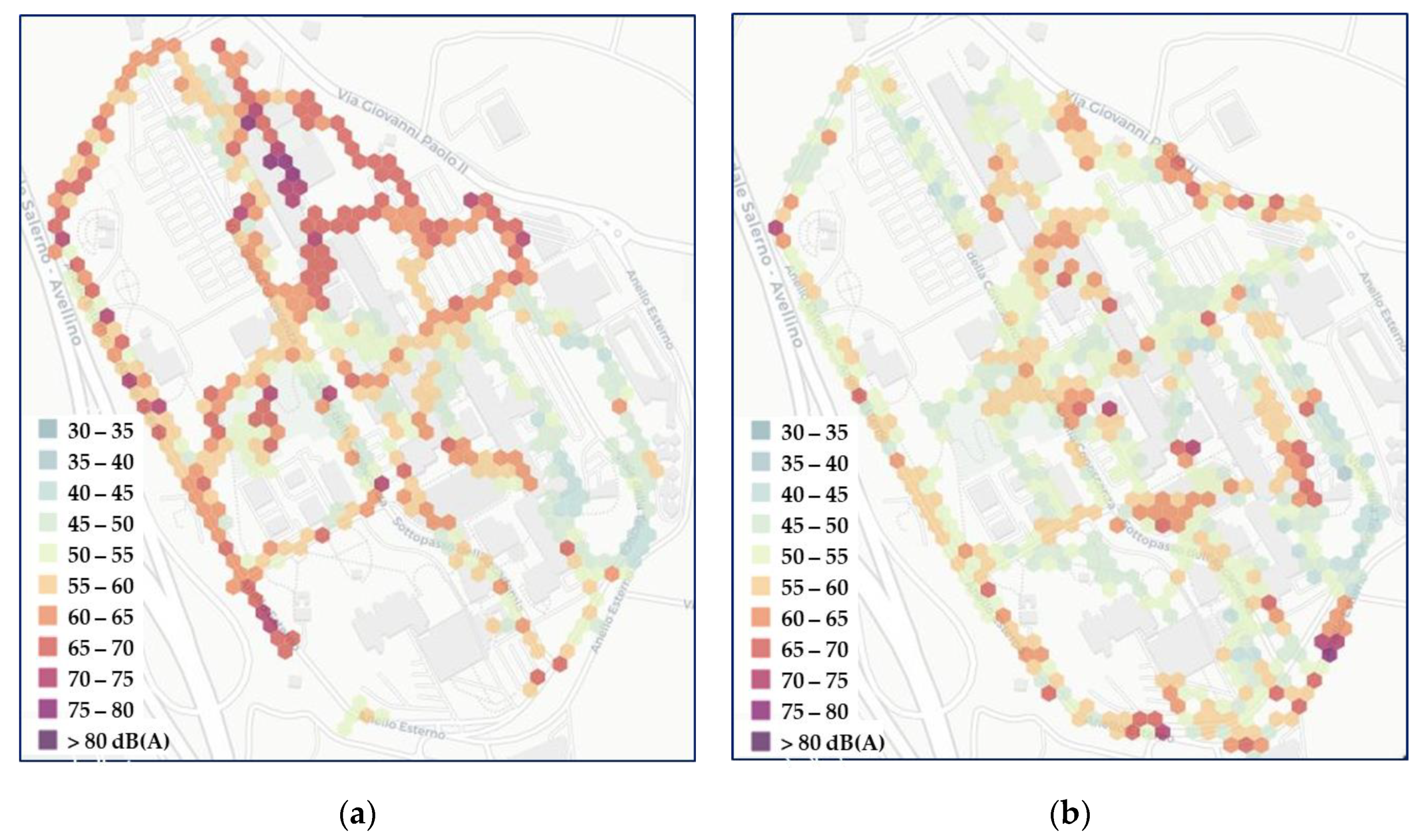
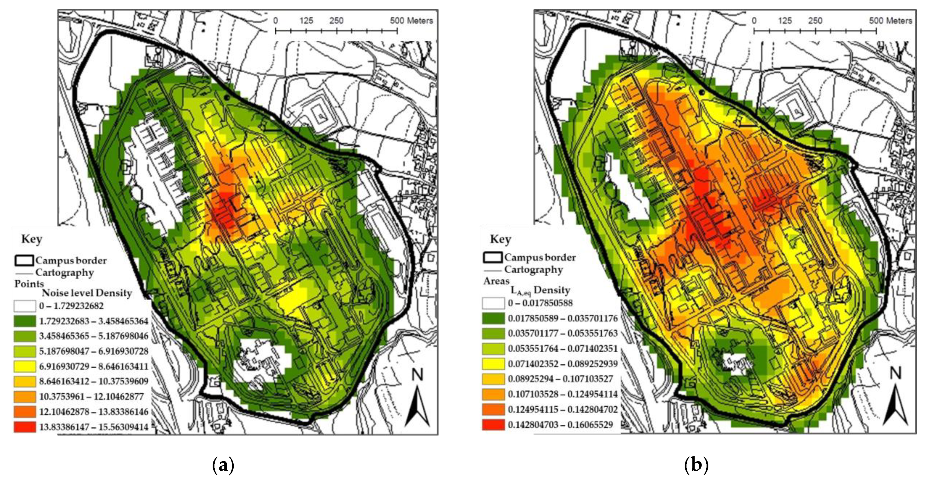
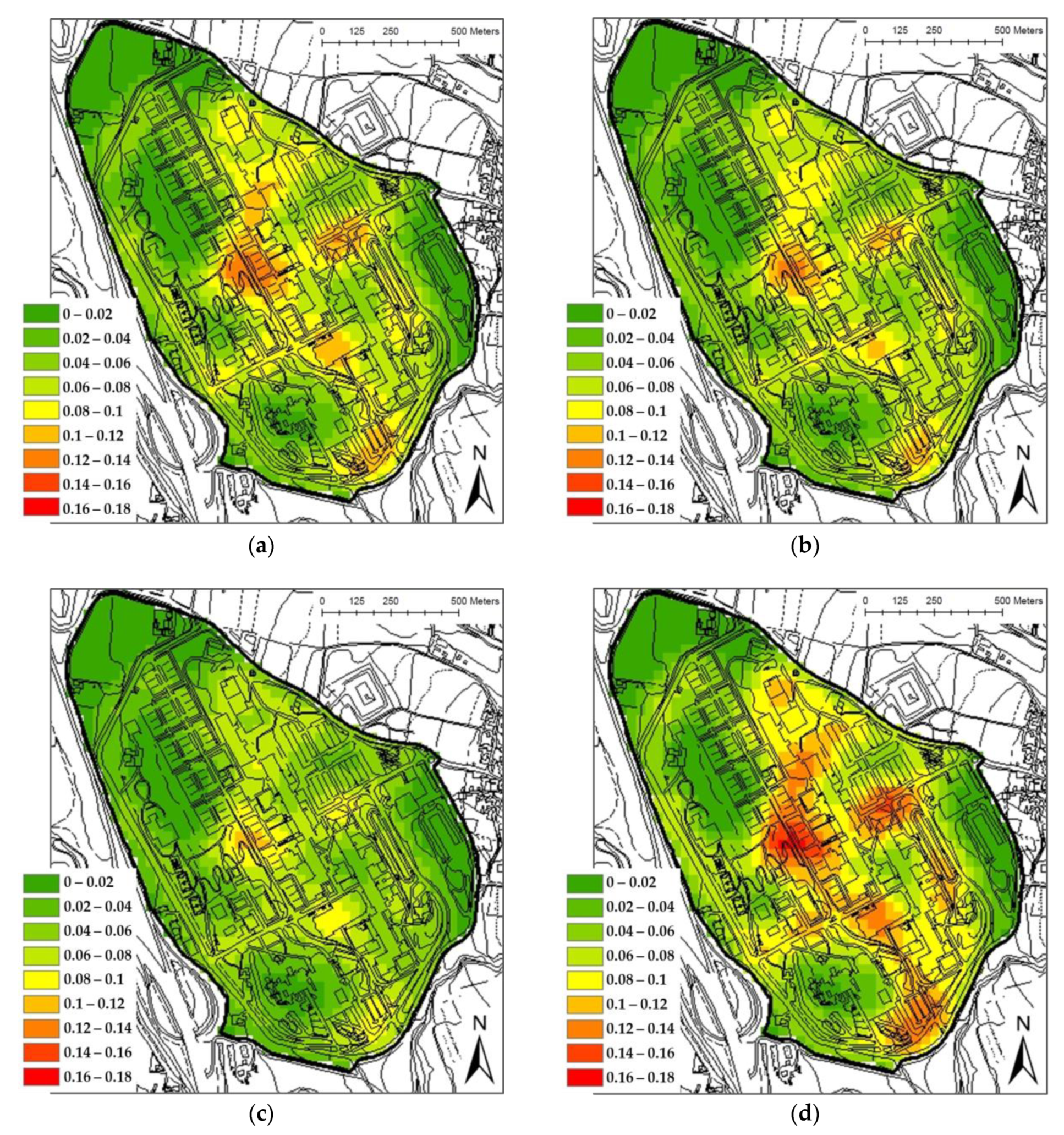
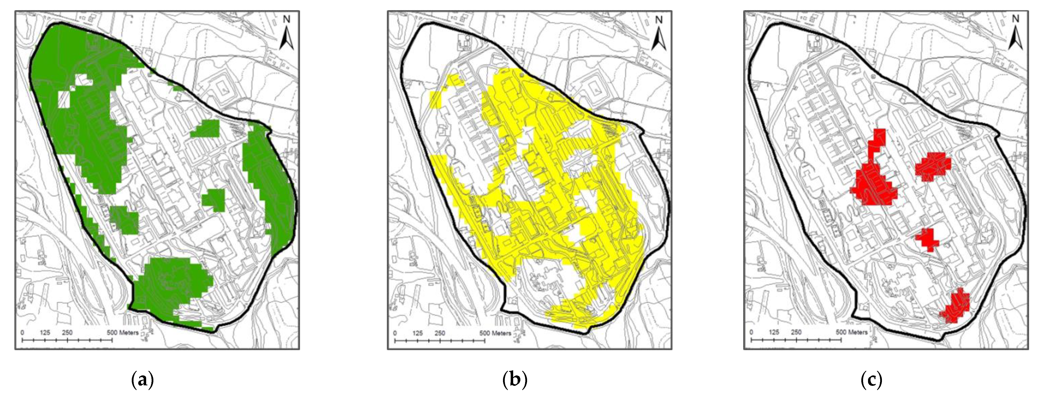
4.1. Creation of Sound Levels Density Maps

From the noise-planet.org website, all the sound level measurements of the Fisciano Campus were acquired on 3 December 2019. Organized in a zipped folder, the files, which can be downloaded for each region of a country, are in .geojson format. Generally, these files are further divided into points and areas, which have specific characteristics in terms of geometry and other information.
The first type, the points file, contains georeferenced points that are characterized by a table of attributes. The relevant fields for this study were the date and time of the measurements and the noise level, i.e., the value of sound pressure level measured at that point in a time of 1 s, expressed in dB(A). The areas file corresponds to basic post-processing of all measurements produced by the community and all data are aggregated in hexagons to produce mean noise indicators and information in each hexagon [62]. The file contains only the hexagons with at least one measurement point belonging to the points file. Its attributes table has several fields, but those relevant for this work are the A-weighted equivalent continuous sound level (LA,eq) and the date and time of the first and the last measurement belonging to the hexagon. The points and areas files were converted into shapefile format and processed in a GIS environment. Figure 5 shows the spatial representation of the noise levels of the points file and the LA,eq of the areas file. Because these maps provide additional information on the acoustic environment, they are not alternative but complementary to the “standard” noise maps, which deal mainly with transport and industrial noise [48].
However, two critical issues can be highlighted from the LA,eq spatial representation. The first problem is related to the spatial non-continuity of the phenomenon between the hexagonal cells, while the second issue concerns the non-homogeneity of the data stored in terms of LA,eq since it is the result of the cumulative measurement points in each hexagon relating to different time intervals.
To overcome the first problem of non-continuity between cells, the kernel density estimation was applied. The outputs were raster maps for each measured parameter, generated in ArcMap© produced by ESRI. For the study case, the function was evaluated considering 100 m for the radius and a 20 m × 20 m cell-sized, with a total area of 400 m2, comparable to the area of the hexagons. Moreover, both the distribution of points relating to the instantaneous measurement of the noise levels (points file) and the distribution of the centroids of the hexagonal cells (areas file) to which LA,eq is associated were used as the basic point pattern (Figure 6). The maps produced were classified using the natural break classification method [66]. Starting from a defined number of classes, this method allows for the identification of the limits of the classes minimizing the internal variance of each class. Accordingly, the representation identifies homogeneous values for each class, highlighting the differences between classes, i.e., representing the intensity of the measurements in terms of noise level and LA,eq.
The difference between the representation of the KDE maps deriving from points and areas that emerge from the values of the classes can be interpreted taking into account that the first map (Figure 6a) follows the instantaneous sampling trajectories, while the second concentrates the point values detected in the center of gravity of each hexagonal cell (Figure 6b). This affects, first, the number of points and, consequently, the value of the KDE which, in the first case, takes on higher min–max values than in the second.
A further difference lies in the spatial variability of the spatial distribution, which is extremely dynamic in the first case because of the variability of the distribution of the measurement points and static in the second because it is related only to the centroids, which are fixed (Figure 7).
To overcome the second problem, a representative map of the acoustic state of the study case, corresponding to a specific day and time, was generated. For this reason, only the hexagons with the last measurement dated 24 May 2019 were selected and saved in a new layer. This choice was made because most of the total data available, corresponding to the last measurements, were collected on that day. Through operations of intersection and summarize in ArcMap©, it is possible to associate the attributes of the points measurements to the hexagons they belong; derive various summary statistics, i.e., average noise level (ANL), minimum noise level (Lmin), and maximum noise level (Lmax); and compare them with the LA,eq, in relation to the density maps respectively generated (Figure 8).
The LA,eq density map was obtained as a function of the continuous equivalent sound pressure level indicator provided by the Noise-Planet platform in the Areas file, and therefore, it is an average time of the pressures measured in each hexagon:
L A , e q = 10 log 10 ( 1 T i = 1 N 10 L A , i 10 )
in which LA,i is the 1-s sound level in dBA recorded by the participants in the i-th point, N is the total number of measurements in each hexagon, and T is the overall measurement time in seconds, which, in our case, is equal to the number of measurements.
The average noise level density map, instead, was obtained as a function of the sound pressure level indicator, i.e., the arithmetic average of the changes in sound pressure measured for each point falling in the hexagon:
A N L = 1 N i = 1 N L A , i
LA,i and N have the same meaning of formula (2).
For qualitative comparison, the two maps can be overlapped and the difference, in terms of percentage, of the single hexagons stands in the order of 0–25%.
A further consideration of this second phase is that the creation of different density maps, representing the spatial distribution of various parameters, should define a protocol for future measurement campaigns necessary to implement the noise maps and monitor the acoustic status of a place. This will be fostered by the calculation in GIS of the LA,eq related to the chosen time interval.
Additionally, ArcMap© allows for the automation of the creation of density maps through a Model Builder application. This creates a sequence of workflows that string together sequences of geoprocessing tools, feeding the output of one tool into another tool as input. It is a parametric model that allows the iteration following a unique analysis protocol. For the study case, the input data were the points and areas shapefiles, while the outputs were four density maps. (Figure 9). This implementation is particularly effective when many measurements are available. Indeed, it is possible to easily spatialize the evolution of the environmental noise phenomenon at various t instants, thus, obtaining multiple density maps at different instants and their comparative evaluations. The considerations that can be reached, for example, through a standard deviation operation, are the identification of the areas in which the phenomenon persists over time with high density and, therefore, the structuring of possible intervention strategies.

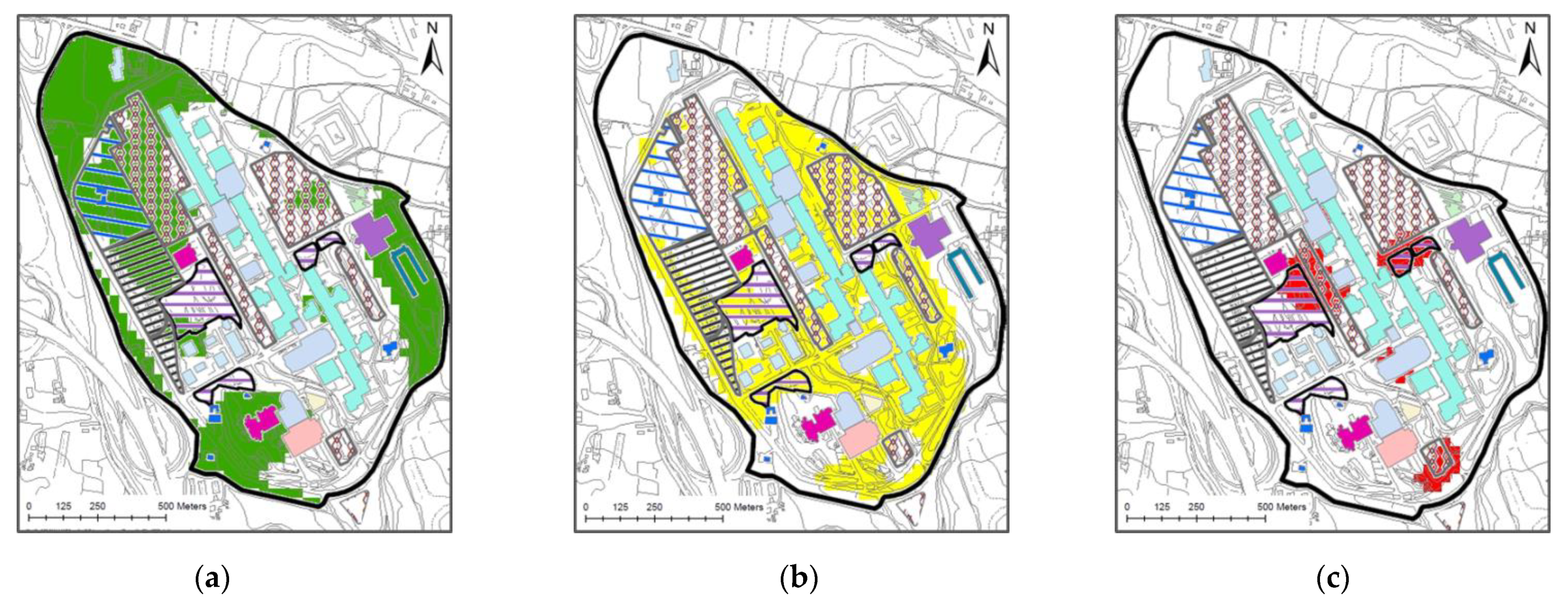
4.2. Noise and Facilities Maps Overlay

Thinking about the relationships between the location of community facilities, the environmental noise, and in general, the impact of urban development on noise generation can lead to the implementation of the third phase of the methodology. It is necessary, indeed, to deepen understanding of the issues related to the application of urban planning parameters to achieve better sound environments and address urban planners in an integrated vision regarding acoustic impacts [67]. This can lead potentially to more effective noise management strategies and, simultaneously, to the sustainability of urban regeneration and transformation.
Currently, the planning of community facilities and services in Italy, also called territorial provisions, is based on strictly quantitative criteria without any reference to the quality of urban settlements. However, in the last decades, the scientific community has been experimenting with new planning approaches that focus on facilities performance and their influence on people’s quality of life and collective wellbeing [67,68]. As highlighted by Gerundo and Graziuso [23], community facilities must be designed specifically for each territorial reality and be open to the effective involvement of citizens in the planning, design, construction, and management of the services. In this framework, the acoustic environment could also become a feature that could influence the choices for the location and management of facilities. The designed methodology, considering volunteers as fundamental characters in the acquisition of acoustic data, integrates the concept that facilities must be planned with the involvement of citizens. The overlay of the noise density maps, with the facilities map, could lead to the identification of appropriate actions for the improvement of the environment, according to the urban and acoustic point of view and people’s evolving needs.
Consequently, the third phase of the methodology was characterized by the identification of all the facilities in the Fisciano Campus according to the main service provided. This allowed for the creation of the community facilities map (Figure 10). As defined previously, this step was made because, on the one hand, the facilities could be considered generators of the pollutant, and on the other, they could be affected by noise.
To interpret the interaction of noise density maps with the community facilities, the ranges of the density values were aggregated into three macro-classes: low (0–0.06), medium (0.07–0.12) and high (0.13–0.18). Therefore, concerning the maximum noise level (Lmax) density map, Figure 11 shows the three new macro-classes.
Through an operation of overlay maps, it has been possible to summarize the relationship between the noise density classes and functions (Figure 12), which led to the compilation of a simple solution matrix of interaction between noise and facilities (Table 2). From the analysis of this matrix, some preliminary considerations can be highlighted. All the facilities with a low effect can be justified because there were few measurements performed in those points. In addition, laboratory L6 was characterized by a low density because it is protected from noise by other buildings and vegetation. Moreover, the theatre; the canteen; the rectorate; the bus station; and most of the squares, teaching buildings, car parks, offices, laboratories, green, and sports facilities were associated with a medium-density class. Three car parks (Cp2, Cp3 and Cp4), two squares (S1 and S3), and the equipped green park (E1) lay partly in the high-density class because of their proximity to the main road axis of the campus. Additionally, the library Li2 and some teaching buildings (T1– T5– T6– T9– T12) partially overlaid the high density class, particularly at the entrance to the facility, because of the presence of a place of high interaction among people, which generally generates an increase of the intensity of noise. The presence of noise generators can be observed also in two equipped green parks (E3 and E4), because of their location in a high overcrowded area that connects the public transport service with most of the buildings.
All these results demonstrate that the solution matrix and the overlay map facilitate the comprehension of the relationship between noise, community facilities, and territorial contexts, thus, becoming useful tools that can support the actions necessary for the reduction of noise exposure. In the planning phase, indeed, such information can support the location choices of new community facilities [23] and organize the urban spaces by localizing the functions that produce impacts and those that experience such pressures [69,70,71,72].

5. Conclusions

In this paper, spatial and temporal density maps of sound pressure levels were generated, starting from data measured by people. According to Citizen Science, the involvement of volunteers for data acquisition contributes to their greater awareness about noise pollution. These geolocated sound level data can also be used for the creation of noise maps, which, opportunely combined with other information, can implement urban planning procedures according to sustainable development standards, as defined by the 2030 agenda. Specifically, the potential of the crowdsourcing data collection tool for the acquisition of information on the noise level has been discussed. Compared with classical noise evaluation methods based on numerical simulations (with a limited number of sound sources and approximated noise propagation models), the noise crowdsourcing platforms have enabled researchers to present a more realistic state of the noise exposure, based on real measurements carried out everywhere. The criticism is only related to the quality of the noise measurement because of smartphone features and their microphone capabilities. However, this limitation can be overcome using post-process measurements.
After the analysis of the various data collection platforms for the sensing environmental noise approach, a methodology for spatial and temporal noise analysis has been defined. It has been organized into three phases, beginning with the acquisition of the data by the experts in the first phase, their analysis and the generation of density maps of the acoustic parameters in the second phase, and the overlay of the density maps with the facilities located in a territory in the third phase.
The methodology was tested in the Fisciano Campus of the University of Salerno, where crowdsourcing noise data collection was organized in 2018 and 2019. As a result of this data, recorded by volunteers and uploaded on the Noise-Planet platform, noise density maps were created in the GIS environment with the use of the kernel density function. Then, through the Model Builder application in the ArcGis© software, it was possible to generate maps, classified according to the established criteria, using input data, suitably adequate and shared by the Noise-Planet platform. The model built becomes an essential tool for further analysis, which involves the study of the phenomenon both spatially and temporally. Moreover, the overlap of these noise density maps with the community facilities of the campus, such as squares, car parks, buildings for education, libraries, and public and equipped green areas, has led to further considerations on the correlation between the sources and the measured levels, which can be used to define the most suitable interventions to be carried out.
Finally, the noise crowdsourcing data could be useful for preserving the acoustic heritage of a place and for pervasive monitoring of noise levels in cities. Consequently, the use of the defined methodology, on different territorial scales, can help to enforce local or regional regulations on limits of the maximum noise levels and become a tool of support both for the actions to be taken to reduce and contain noise and for the location choices of the urban transformations.

Author Contributions

Conceptualization, G.G., M.G. and C.G.; methodology, G.G., S.M., A.B.F., M.G. and C.G.; software, G.G. and M.G.; validation, G.G., S.M., A.B.F., M.G. and C.G.; formal analysis, G.G., S.M., A.B.F., M.G. and C.G.; investigation, G.G., S.M., A.B.F., M.G. and C.G.; data curation, G.G. and M.G.; writing—original draft preparation, G.G.; writing—review and editing, G.G., S.M., A.B.F., M.G. and C.G.; supervision, C.G. All authors have read and agreed to the published version of the manuscript.

Funding

This research received no external funding.

Data Availability Statement

The datasets used in this paper were collected within the NoiseCapture project [68] and were downloaded from https://data.noise-planet.org/index.html (accessed on 13 May 2021). They are distributed under the open database license (ODbL) terms.

Acknowledgments

The authors are grateful to Letizia Leva for contributing to this research during her bachelor thesis. The authors also acknowledge the contribution of the students of the first year of the Civil Engineering and Environmental Engineering program of the University of Salerno who participated in the “NoiseCapture parties”, collecting the data used in this work.

Conflicts of Interest

The authors declare no conflict of interest.

References

  1. Schwela, D. Environmental Noise Challenges and Policies in Low—and Middle—Income Countries. South. Fla. J. Health. 2021, 2, 26–45. [Google Scholar] [CrossRef]
  2. Basner, M.; Babisch, W.; Davis, A.; Brink, M.; Clark, C.; Janssen, S.; Stansfeld, S. Auditory and Non-Auditory Effects of Noise on Health. Lancet 2014, 383, 1325–1332. [Google Scholar] [CrossRef] [Green Version]
  3. European Environment Agency. The European Environment—State and Outlook 2020: Knowledge for Transition to a Sustainable Europe. Available online: www.eea.europa.eu/publications/soer-2020 (accessed on 2 February 2021).
  4. Berglund, B.; Lindvall, T.; Schwela, D.; Dietrich, H.; World Health Organization. Occupational and Environmental Health Team. Guidelines for Community Noise. 1999. Available online: apps.who.int/iris/handle/10665/66217 (accessed on 2 February 2021).
  5. World Health Organization. Environmental Noise Guidelines for the European Region. 2018. Available online: www.euro.who.int/en/publications/abstracts/environmental-noise-guidelines-for-the-european-region-2018 (accessed on 2 February 2021).
  6. European Union. Directive 2002/49/EC of the European parliament and the Council of 25 June 2002 relating to the assessment and management of environmental noise. Off. J. Eur. Communities. 2002, 189, 12–25. [Google Scholar]
  7. Kephalopoulos, S.; Paviotti, M.; Anfosso-Lédée, F. Common Noise Assessment Methods in Europe (CNOSSOS-EU). In EUR25379EN; Publications Office of the European Union: Luxembourg, 2012. [Google Scholar]
  8. Guarnaccia, C.; Quartieri, J.; Tepedino, C.; Rodrigues, E.R. A Time Series Analysis and a Non-Homogeneous Poisson Model with Multiple Change-Points Applied to Acoustic Data. Appl. Acoust. 2016, 114, 203–212. [Google Scholar] [CrossRef]
  9. Guarnaccia, C. Advanced Tools for Traffic Noise Modelling and Prediction. WSEAS Trans. Syst. 2013, 12, 121–130. [Google Scholar]
  10. Guarnaccia, C. EAgLE: Equivalent acoustic level estimator proposal. Sensors. 2020, 20, 701. [Google Scholar] [CrossRef] [PubMed] [Green Version]
  11. Guarnaccia, C.; Quartieri, J. Analysis of Road Traffic Noise Propagation. Int. J. Math. Mod. Meth. Appl. Sci. 2012, 6, 926–933. [Google Scholar]
  12. Iannone, G.; Guarnaccia, C.; Quartieri, J. Noise Fundamental Diagram Deduced by Traffic Dynamics. In Proceedings of the 4th WSEAS International Conference on EMESEG’11, Corfu Island, Greece, 14–16 July 2011; pp. 501–507. [Google Scholar]
  13. Benocci, R.; Confalonieri, C.; Roman, H.E.; Angelini, F.; Zambon, G. Accuracy of the Dynamic Acoustic Map in a Large City Generated by Fixed Monitoring Units. Sensors 2020, 20, 412. [Google Scholar] [CrossRef] [PubMed] [Green Version]
  14. Aumond, P.; Jacquesson, L.; Can, A. Probabilistic Modeling Framework for Multisource Sound Mapping. Appl. Acoust. 2018, 139, 34–43. [Google Scholar] [CrossRef] [Green Version]
  15. Steele, C. A Critical Review of Some Traffic Noise Prediction Models. Appl. Acoust. 2001, 62, 271–287. [Google Scholar] [CrossRef]
  16. Can, A.; Aumond, P. Estimation of Road Traffic Noise Emissions: The Influence of Speed and Acceleration. Transport. Res. D-Tr E. 2018, 58, 155–171. [Google Scholar] [CrossRef]
  17. Guillaume, G.; Can, A.; Petit, G.; Fortin, N.; Palominos, S.; Gauvreau, B.; Bocher, E.; Picaut, J. Noise Mapping Based on Participative Measurements. Noise Mapp. 2016, 3, 140–156. [Google Scholar] [CrossRef] [Green Version]
  18. Sakagami, K.; Satoh, F.; Omoto, A. Use of Mobile Devices with Multifunctional Sound Level Measurement Applications. Some Experiences for Urban Acoustics Education in Primary and Secondary Schools. Urban. Sci. 2019, 3, 111. [Google Scholar] [CrossRef]
  19. Cuff, D.; Hansen, M.; Kang, J. Urban Sensing: Out of the Woods. Commun. Assoc. Comput. Mach. 2008, 51, 24–33. [Google Scholar] [CrossRef]
  20. Picaut, J.; Fortin, N.; Bocher, E.; Petit, G.; Aumond, P.; Guillaume, G. An Open-Science Crowdsourcing Approach for Producing Community Noise Maps Using Smartphones. Build. Environ. 2019, 148, 20–33. [Google Scholar] [CrossRef]
  21. Hammad, A.W.A.; Akbarnezhad, A.; Rey, D. Sustainable Urban Facility Location: Minimising Noise Pollution and Network Congestion. Transp. Res. E-Log. 2017, 107, 38–59. [Google Scholar] [CrossRef]
  22. United Nations. The 17 Goals. Available online: sdgs.un.org/goals (accessed on 11 February 2021).
  23. Gerundo, R.; Graziuso, G. The Performance Evaluation of Community Facilities and Services. Archivio Studi Urbani Regionali 2020, (Suppl. S127), 113–129. [Google Scholar] [CrossRef]
  24. Adams, M.; Cox, T.; Moore, G.; Croxford, B.; Refaee, M.; Sharples, S. Sustainable Soundscapes: Noise Policy and the Urban Experience. Urban. Stud. 2006, 43, 2385–2398. [Google Scholar] [CrossRef]
  25. Melachrinoudis, E. Bicriteria Location of a Semi-Obnoxious Facility. Comput. Ind. Eng. 1999, 37, 581–593. [Google Scholar] [CrossRef]
  26. Statista. Available online: www.statista.com/statistics/330695/number-of-smartphone-users-worldwide/ (accessed on 29 January 2021).
  27. Swan, M. Crowdsourced Health Research Studies: An Important Emerging Complement to Clinical Trials in the Public Health Research Ecosystem. J. Med. Internet Res. 2012, 14, e46. [Google Scholar] [CrossRef]
  28. Conrad, C.C.; Hilchey, K.G. A Review of Citizen Science and Community-Based Environmental Monitoring: Issues and Opportunities. Environ. Monit. Assess. 2011, 176, 273–291. [Google Scholar] [CrossRef] [PubMed]
  29. European Union. Directive 2003/35/EC of the European Parliament and of the Council of 26 May 2003 Providing for Public Participation in Respect of the Drawing Up of Certain Plans and Programs Relating to the Environment and Amending with Regard to Public Participation and Access to Justice Council Directives 85/337/EEC and 96/61/EC. Off. J. Eur. Union. 2003, 156, 17. [Google Scholar]
  30. Soleimani, S.; Keshtehgar, E.; Reza Malek, M. Ubisound: Design a User Generated Model in Ubiquitous Geospatial Information Environment for Sound Mapping. Int. Arch. Photogramm. 2014, XL-2/W3, 243–247. [Google Scholar] [CrossRef] [Green Version]
  31. Stevens, M.; D’Hondt, E. Crowdsourcing of Pollution Data Using Smartphones. In Proceedings of the ACM conference on Ubiquitous Computing 2010 (UbiComp2010), Copenhagen, Denmark, 26–29 September 2010. [Google Scholar]
  32. Stevens, M. Community Memories for Sustainable Societies: The Case of Environmental Noise. Ph.D. Thesis, Faculty of Science and Bio-Engineering Sciences, Vrije Universiteit, Brussel, Belgium, June 2012. [Google Scholar]
  33. Becker, M.; Caminiti, S.; Fiorella, D.; Francis, L.; Gravino, P.; Haklay, M.; Hotho, A.; Loreto, V.; Mueller, J.; Ricchiuti, F.; et al. Awareness and Learning in Participatory Noise Sensing. PLoS ONE 2013, 8, e81638. [Google Scholar] [CrossRef] [Green Version]
  34. Kanjo, E. NoiseSPY: A Real-Time Mobile Phone Platform for Urban Noise Monitoring and Mapping. Mob. Netw. Appl. 2010, 15, 562–574. [Google Scholar] [CrossRef] [Green Version]
  35. Malatras, A.; Peng, F.; Hirsbrunner, B. BioMPE: Definition of Network Characteristics and Cross-Layer Interfaces; Technical Report; Department of Informatics, University of Fribourg: Fribourg, Switzerland, 2012. [Google Scholar]
  36. Ruge, L.; Altakrouri, B.; Schrader, A. SoundOfTheCity—Continuous Noise Monitoring for a Healthy City. In Proceedings of the 2013 IEEE International Conference (PERCOM Workshops), San Diego, CA, USA, 18–22 March 2013; pp. 670–675. [Google Scholar]
  37. Schweizer, I.; Probst, F.; Bärtl, R.; Mühlhäuser, M.; Schulz, A. NoiseMap—Real-time Participatory Noise Maps. In Proceedings of the 2nd International Workshop on Sensing Applications on Mobile Phones, Seattle, WA, USA, 1–4 November 2011. [Google Scholar]
  38. Garcia-Martí, I.; Rodríguez-Pupo, L.E.; Benedito, M.; Trilles, S.; Beltran, A.; Díaz, L.; Huerta, J. Mobile Application for Noise Pollution Monitoring through Gamification Techniques. In Lecture Notes in Computer Science, Proceedings of the 11th International Conference (ICEC 2012), Bremen, Germany, 26–29 September 2012; Springer: Berlin/Heidelberg, Germany, 2012; Volume 7522, pp. 562–571. [Google Scholar]
  39. Garcia-Martí, I.; Rodríguez-Pupo, L.E.; Díaz, L.; Huerta, J. Noise Battle: A Gamified application for Environmental Noise Monitoring in Urban Areas. In Proceedings of the 16th AGILE Conf. on Geographic Information Science (AGILE 2013), Geographic Information Science at the Heart of Europe, Leuven, Belgium, 14–17 May 2013. [Google Scholar]
  40. Noise Planet Project Website. Available online: noise-planet.org/index.html (accessed on 27 April 2021).
  41. ARPA Piemonte. Available online: www.arpa.piemonte.it/approfondimenti/temi-ambientali/rumore/rumore/openoise-2 (accessed on 29 January 2021).
  42. King, G.; Roland-Mieszkowski, M.; Jason, T.; Rainham, D.G. Noise Levels Associated with Urban Land Use. J. Urban. Health. 2012, 89, 1017–1030. [Google Scholar] [CrossRef] [PubMed] [Green Version]
  43. Pueh Lee, H.; Garg, S.; Meng Lim, K. Crowdsourcing of Environmental Noise Map Using Calibrated Smartphones. Appl. Acoust. 2020, 160, 107130. [Google Scholar]
  44. Maisonneuve, N.; Stevens, M.; Ochab, B. Participatory Noise Pollution Monitoring Using Mobile Phones. Inform. Polity 2010, 15, 51–71. [Google Scholar] [CrossRef] [Green Version]
  45. Bocher, E.; Petit, G.; Fortin, N.; Picaut, J.; Guillaume, G.; Palominos, S. OnoM@p: A Spatial Data Infrastructure Dedicated to Noise Monitoring Based on Volunteers Measurements. PeerJ Prepr. 2016, 4, e2273v2. [Google Scholar] [CrossRef]
  46. Drosatos, G.; Efraimidis, P.S.; Athanasiadis, I.N.; Stevens, M.; D’Hondt, E. Privacy-Preserving Computation of Participatory Noise Maps in the Cloud. J. Syst. Softw. 2014, 92, 170–183. [Google Scholar] [CrossRef]
  47. Zamora, W.; Calafate, C.T.; Cano, J.C.; Manzoni, P. Accurate Ambient Noise Assessment Using Smartphones. Sensors 2017, 17, 917. [Google Scholar] [CrossRef] [Green Version]
  48. Brambilla, G.; Pedrielli, F. Smartphone-Based Participatory Soundscape Mapping for a More Sustainable Acoustic Environment. Sustainability 2020, 12, 7899. [Google Scholar] [CrossRef]
  49. Sakagami, K.; Satoh, F.; Omoto, A. Revisiting Acoustics Education Using Mobile Devices to Learn Urban Acoustic Environments: Recent Issues on Current Devices and Applications. Urban. Sci. 2019, 3, 73. [Google Scholar] [CrossRef] [Green Version]
  50. D’Hondt, E.; Stevens, M.; Jacobs, A. Participatory Noise Mapping Works! An Evaluation of Participatory Sensing as an Alternative to Standard Techniques for Environmental Monitoring. Pervasive Mob. Comput. 2013, 9, 681–694. [Google Scholar] [CrossRef]
  51. Zuo, J.; Xia, H.; Liu, S.; Qiao, Y. Mapping Urban Environmental Noise Using Smartphones. Sensors 2016, 16, 1692. [Google Scholar] [CrossRef] [Green Version]
  52. Murphy, E.; King, E.A. Testing the Accuracy of Smartphones and Sound Level Meter Applications for Measuring Environmental Noise. Appl. Acoust. 2016, 106, 16–22. [Google Scholar] [CrossRef] [Green Version]
  53. D’Hondt, E.; Stevens, M. Participatory Noise Mapping. In Proceedings of the 9th International Conference on Pervasive Computing (Pervasive ‘11), San Francisco, CA, USA, 12–15 June 2011. [Google Scholar]
  54. Aumond, P.; Lavandier, C.; Ribeiro, C.; Boix, E.G.; Kambona, K.; D’Hondt, E.; Delaitre, P. A Study of the Accuracy of Mobile Technology for Measuring Urban Noise Pollution in Large Scale Participatory Sensing Campaigns. Appl. Acoust. 2017, 117, 219–226. [Google Scholar] [CrossRef]
  55. Can, A.; Dekoninck, L.; Botteldooren, D. Measurement Network for Urban Noise Assessment: Comparison of Mobile Measurements and Spatial Interpolation Approaches. Appl. Acoust. 2014, 83, 32–39. [Google Scholar] [CrossRef] [Green Version]
  56. Grubeša, S.; Petošic´, A.; Suhanek, M.; Ðurek, I. Mobile Crowdsensing Accuracy for Noise Mapping in Smart Cities. Automatika 2018, 59, 286–293. [Google Scholar] [CrossRef] [Green Version]
  57. Tobler, W. A Computer Movie Simulating Urban Growth in the Detroit Region. Econ. Geogr. 1970, 46 (Suppl. S1), 234–240. [Google Scholar] [CrossRef]
  58. Gatrell, A.C.; Bailey, T.C.; Diggle, P.J.; Rowlingson, B.S. Spatial Point Pattern Analysis and its Application in Geographical Epidemiology. Trans. Inst. Br. Geogr. 1996, 21, 256–274. [Google Scholar] [CrossRef]
  59. Bailey, T.C.; Gatrell, A.C. Interactive Spatial Data Analysis; Longman Scientific & Technical: Harlow, UK, 1995; Volume 413. [Google Scholar]
  60. Sebillo, M.; Tucci, M.; Tortora, G.; Vitiello, G.; Ginige, A.; Di Giovanni, P. Combining Personal Diaries with Territorial Intelligence to Empower Diabetic Patients. J. Vis. Lang. Comput. 2015, 29, 1–14. [Google Scholar] [CrossRef]
  61. Grimaldi, M.; Sebillo, M.; Vitiello, G.; Pellecchia, V. Planning and Managing the Integrated Water System: A Spatial Decision Support System to Analyze the Infrastructure Performances. Sustainability 2020, 12, 6432. [Google Scholar] [CrossRef]
  62. Sebillo, M.; Vitiello, G.; Grimaldi, M.; Dello Buono, S. SAFE (Safety for Families in Emergency): A Citizen-Centric Approach for Risk Management. In Computational Science and Its Applications—ICCSA 2019—Part II. Lecture Notes in Computer Science, Proceedings of the 19th International Conference, Saint Petersburg, Russia, 1–4 July 2019; Misra, S., Gervasi, O., Murgante, B., Stankova, E., Korkhov, V., Torre, C., Rocha, A.A.A.C., Taniar, D., Apduhan, B.O., Tarantino, E., Eds.; Springer: Berlin/Heidelberg, Germany, 2019; Volume 11620. [Google Scholar]
  63. Sebillo, M.; Vitiello, G.; Paolino, L.; Ginige, A. Training Emergency Responders through Augmented Reality Mobile Interfaces. Multimed Tools Appl. 2016, 75, 9609–9622. [Google Scholar] [CrossRef]
  64. Kenchington, E.; Murillo, F.J.; Lirette, C.; Sacau, M.; Koen-Alonso, M.; Kenny, A.; Ollerhead, N.; Wareham, V.; Beazleyet, L. Kernel Density Surface Modelling as a Means to Identify Significant Concentrations of Vulnerable Marine Ecosystem Indicators. PLoS ONE 2014, 9, 1–14. [Google Scholar] [CrossRef]
  65. Mancini, S.; Mascolo, A.; Graziuso, G.; Guarnaccia, C. Soundwalk, Questionnaires and Noise Measurements in a University Campus: A Soundscape Study. Sustainability 2021, 13, 841. [Google Scholar] [CrossRef]
  66. Jenks, G.F. The Data Model Concept in Statistical Mapping. Int. Yearb. Cartogr. 1967, 7, 186–190. [Google Scholar]
  67. Tong, H.; Kang, J. Relationship Between Urban Development Patterns and Noise Complaints in England. Environ. Plann. B. Urban Anal. City Sci. 2020, 1–18. [Google Scholar] [CrossRef]
  68. Bocher, E.; Petit, G.; Picaut, J.; Fortin, N.; Guillaume, G. Collaborative Noise Data Collected from Smartphones. Data Brief. 2017, 14, 498–503. [Google Scholar] [CrossRef]
  69. Gerundo, R.; Marra, A.; De Salvatore, V. Construction of a Composite Vulnerability Index to Map Peripheralization Risk in Urban and Metropolitan Areas. Sustainability 2020, 12, 4641. [Google Scholar] [CrossRef]
  70. Sicignano, E.; Di Ruocco, G.; Stabile, A. Quali—A Quantitative Environmental Assessment Method According to Italian CAM, for the Sustainable Design of Urban Neighbourhoods in Mediterranean Climatic Regions. Sustainability 2019, 11, 4603. [Google Scholar] [CrossRef] [Green Version]
  71. Fasolino, I.; Coppola, F.; Grimaldi, M. A Model for Urban Planning Control of the Settlement Efficiency. A Case Study. Arch. Studi Urbani Reg. 2020, (Suppl. S127), 181–210. [Google Scholar] [CrossRef]
  72. Vilaça, M.; Macedo, E.; Tafidis, P.; Coelho, M.C. Multinomial Logistic Regression for Prediction of Vulnerable Road Users Risk Injuries Based on Spatial and Temporal Assessment. Int. J. Inj. Control Saf. Promot. 2019, 26, 379–390. [Google Scholar] [CrossRef] [PubMed]
Figure 1. Kernel density estimation [58] (courtesy of JSTOR).
Sustainability 13 05486 g001
Figure 2. The 3–phases noise analysis model.
Sustainability 13 05486 g002
Figure 3. The spatial framework of Fisciano Campus—University of Salerno (Italy).
Sustainability 13 05486 g003
Figure 4. University of Salerno NoiseCapture Party Maps—(a) 17/05/2018; (b) 24/05/2019 (noise-planet.org, ODbL).
Sustainability 13 05486 g004
Figure 5. Spatial representation of all measurements of (a) noise level and (b) LA,eq.
Sustainability 13 05486 g005
Figure 6. Density maps deriving from: (a) points measurements; (b) areas measurements.
Sustainability 13 05486 g006
Figure 7. Spatial distribution of: (a) points; (b) centroids of areas.
Sustainability 13 05486 g007
Figure 8. Density maps referred to NoiseCapture Party—24/05/2019: (a) LA,eq; (b) ANL; (c) Lmin; (d) Lmax.
Sustainability 13 05486 g008
Figure 9. Model Builder for the elaboration of noise maps.
Sustainability 13 05486 g009
Figure 10. University of Salerno—Community Facilities Map.
Sustainability 13 05486 g010
Figure 11. Macro-classes of Lmax: (a) Low-density; (b) Medium-density; (c) High-density.
Sustainability 13 05486 g011
Figure 12. Overlay map of Lmax density macro-classes and facilities: (a) Low effect; (b) Medium effect; (c) High effect.
Sustainability 13 05486 g012
Table 1. Participatory tools and functionality for environmental noise assessment. The ✓ symbol refers to a feature fully implemented, the * symbol means that the feature is partially implemented and needs future improvements and the - symbol is for non implemented features. Modified from [17,30,36].
ApplicationsFeatures 1
PECERAUCAEEConPNCSCCalS/IEACor
SoundOfTheCity---**
NoiseTube------
NoiseSpy-**---*
Ear-Phone*-*----
WideNoise---*------*
NoiseMap----------
MobGeoSen----**------*
NoiseBattle----------
NoiseTubePrime-------
UbiSound----
Laermometer-----------
NoiseDroid------------
2Loud?*---------
NoizCrowd--------*-
NoiseWatch----------
OpeNoise------
NoiseCapture---
1 PE = personal exposure; CE = community exposure; RA = risk assessment; U = unobtrusiveness; CA = context awareness; EE = experience exposure; Con = continuity; P = privacy; NC = noise capture; SC = soundscape capture; Cal = calibration; S/I = standards/interoperability; EA = energy awareness; Cor = correctness.
Table 2. Solution Matrix: Facilities/noise density classes. The numbers refer to the locations of facilities showed in Figure 10; the ✓ symbol means that there is only one facility in the campus and it falls within the class indicated.
FacilitiesNoise Density Classes
LowMediumHigh
Theatre--
Canteen-
Laboratory—LnL1, L6L2, L3, L4, L5, L7, L8-
Office—OnO1, O2, O3, O4, O7, O8O2, O3, O4, O5, O6-
Library—LinLi1, Li2Li2Li2
Rectorate-
Car park—CpnCp1, Cp2Cp1, Cp2, Cp3, Cp4, Cp5Cp2, Cp3, Cp4
Teaching building—TnT1, T4, T8, T9T1, T2, T3, T4, T5, T6, T7, T8, T9, T10, T11, T12T1, T5, T6, T9, T12
Green park-
Equipped green park—EnE1E1, E2E1, E3, E4
Sport facility-
Public square—SnS4S1, S2, S3, S4, S5, S6S1, S3
Student residence--
Bus station--
Publisher’s Note: MDPI stays neutral with regard to jurisdictional claims in published maps and institutional affiliations.

