
Volumetric Quantification of Flash Flood Using Microwave Data on a Watershed Scale in Arid Environments, Saudi Arabia

 ,
,  , and
, and 
Abstract
:1. Introduction
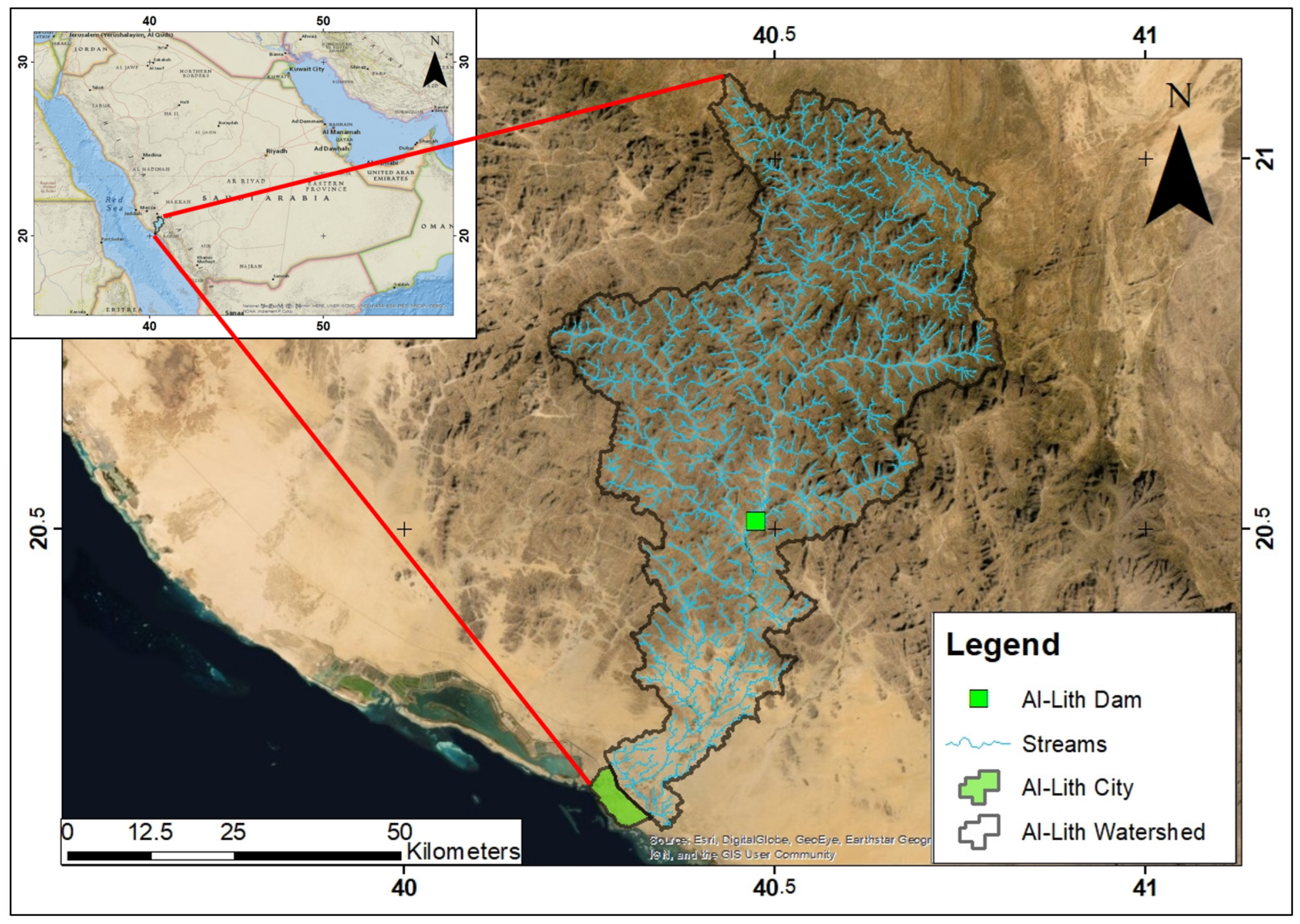
2. Study Area
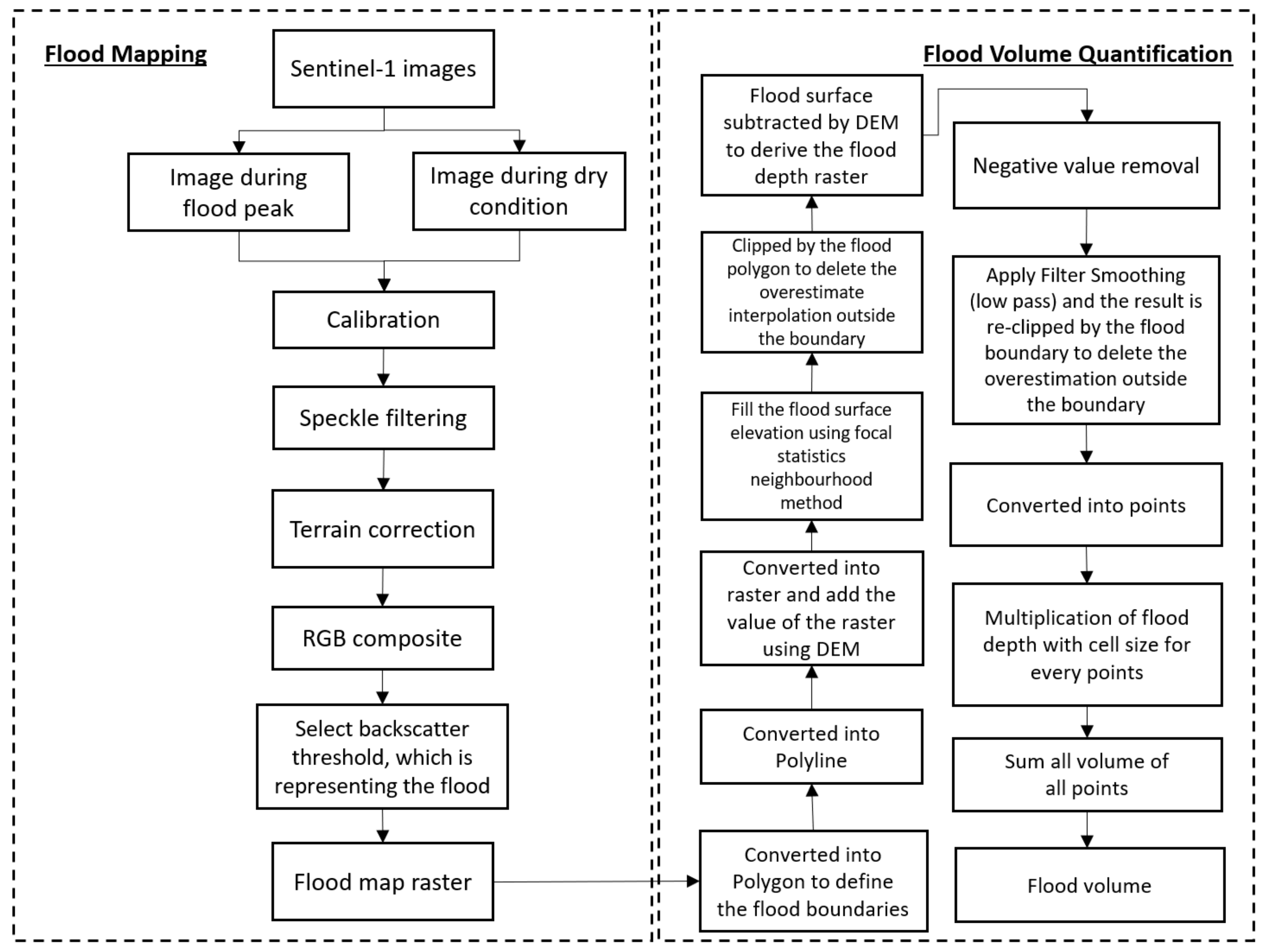
3. Methodological Framework
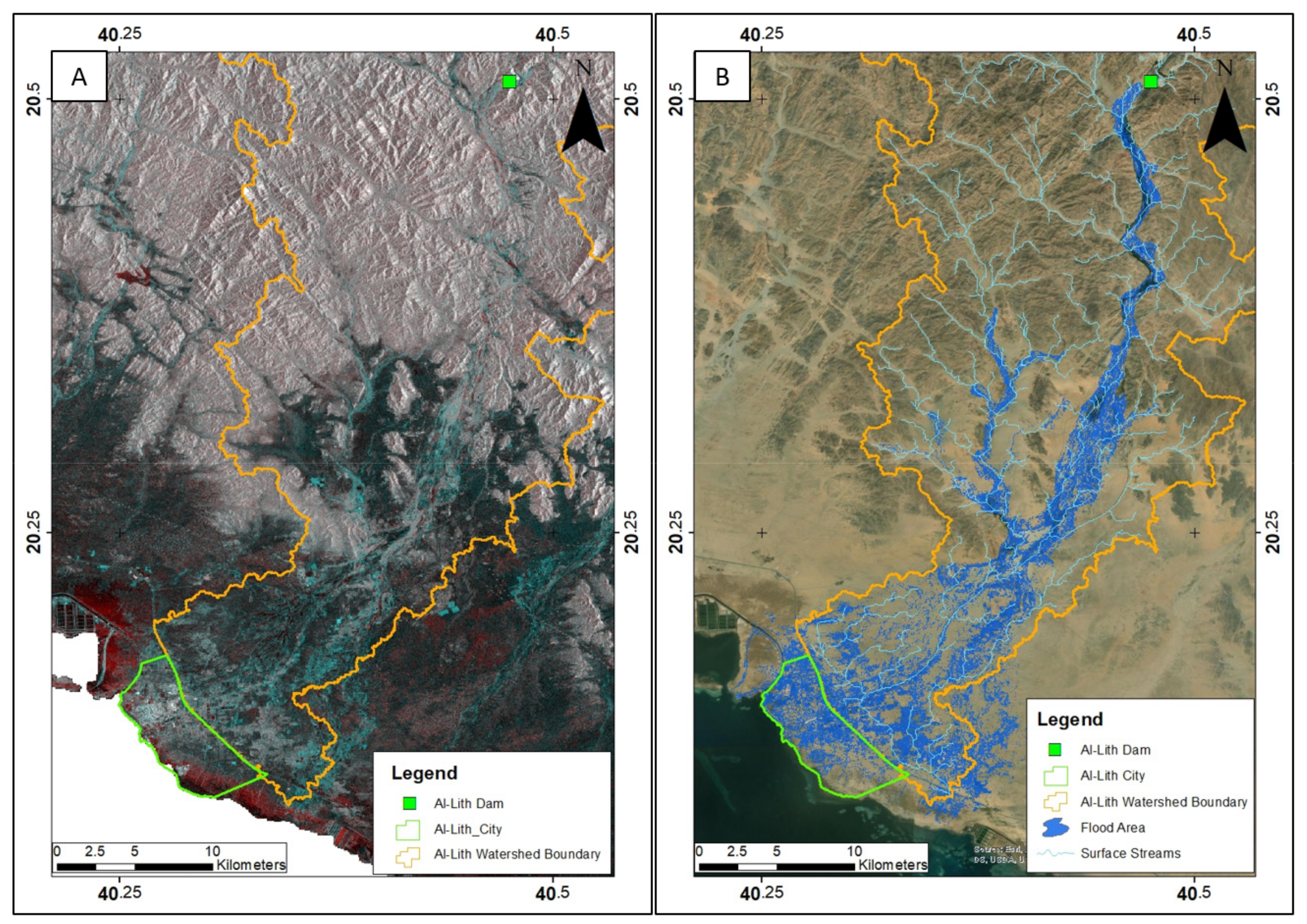
3.1. Flash Flood Mapping
- Calibration and radiometric correction
- Speckle filtering
- Terrain correction
- Create stack and RGB composite
3.2. Flood Volume Quantification
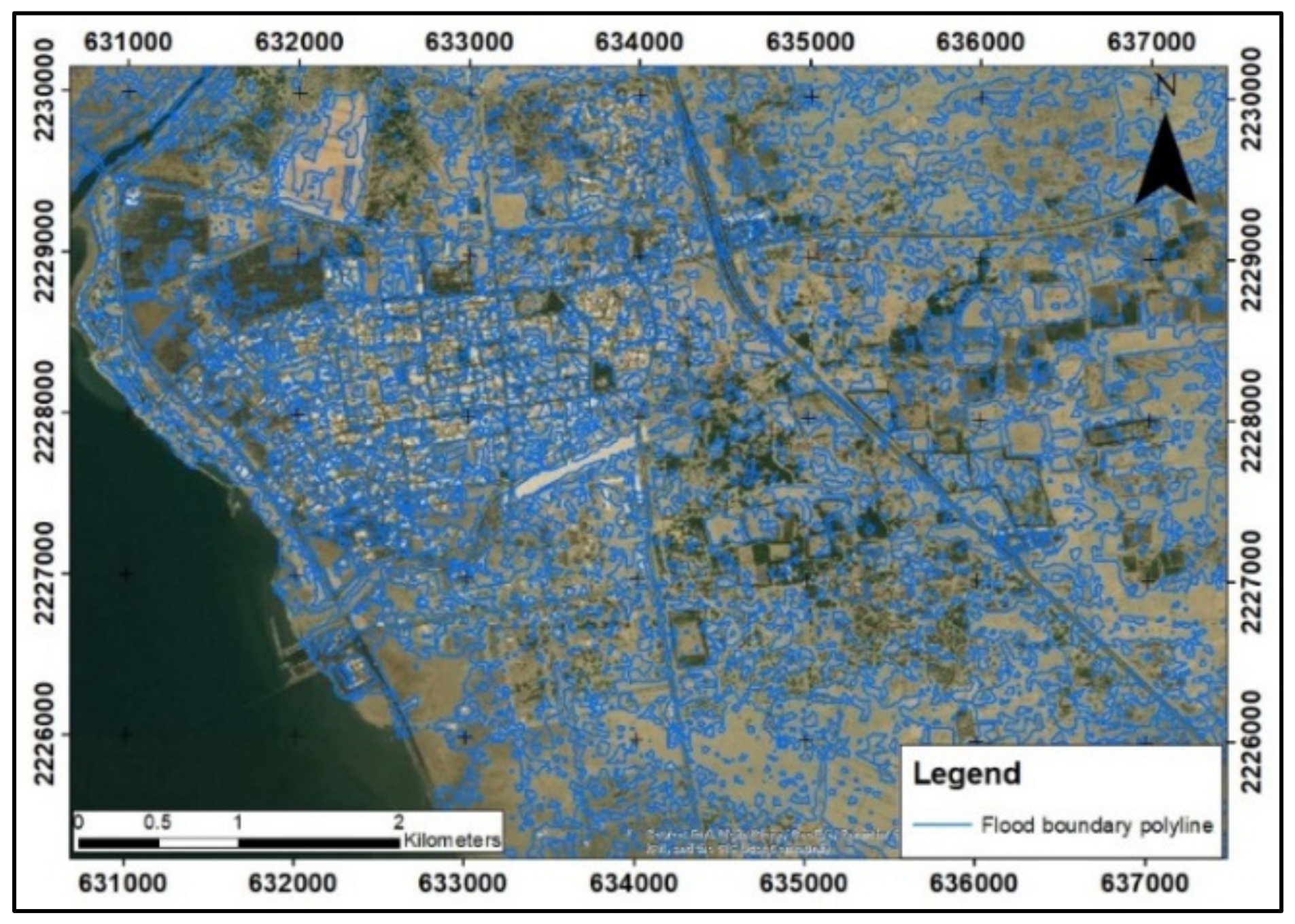
- Define the flood boundary
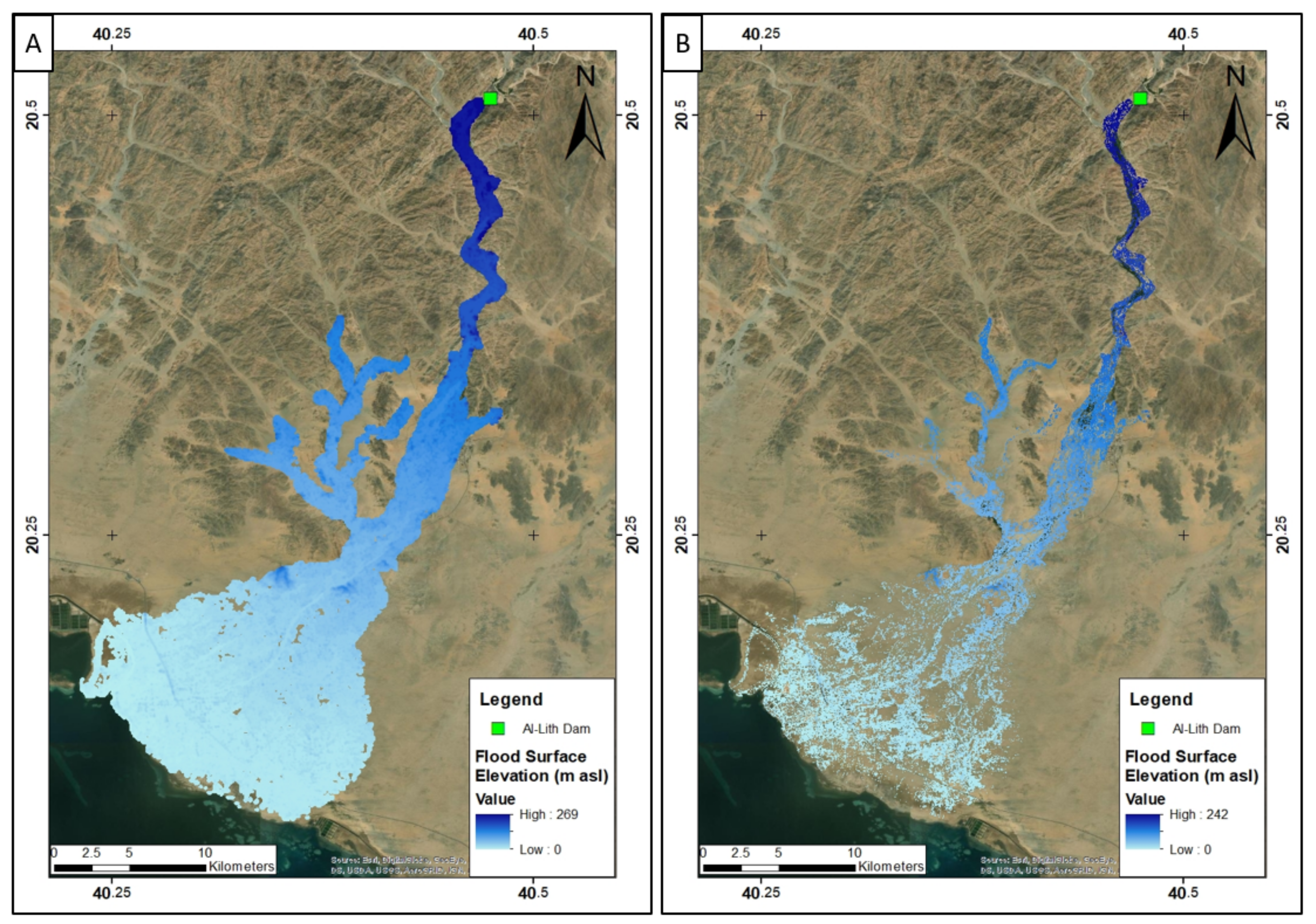
- Define the flood surface elevation
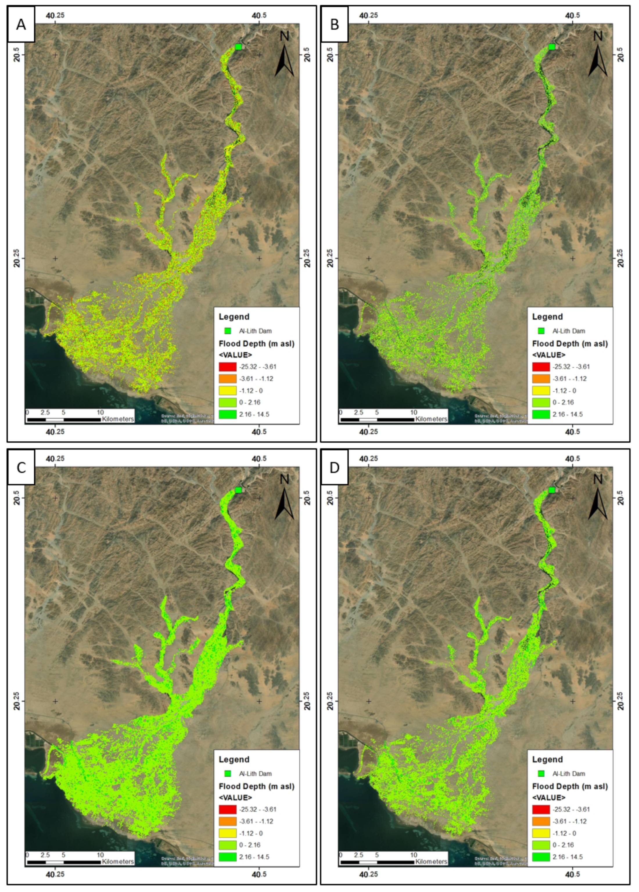
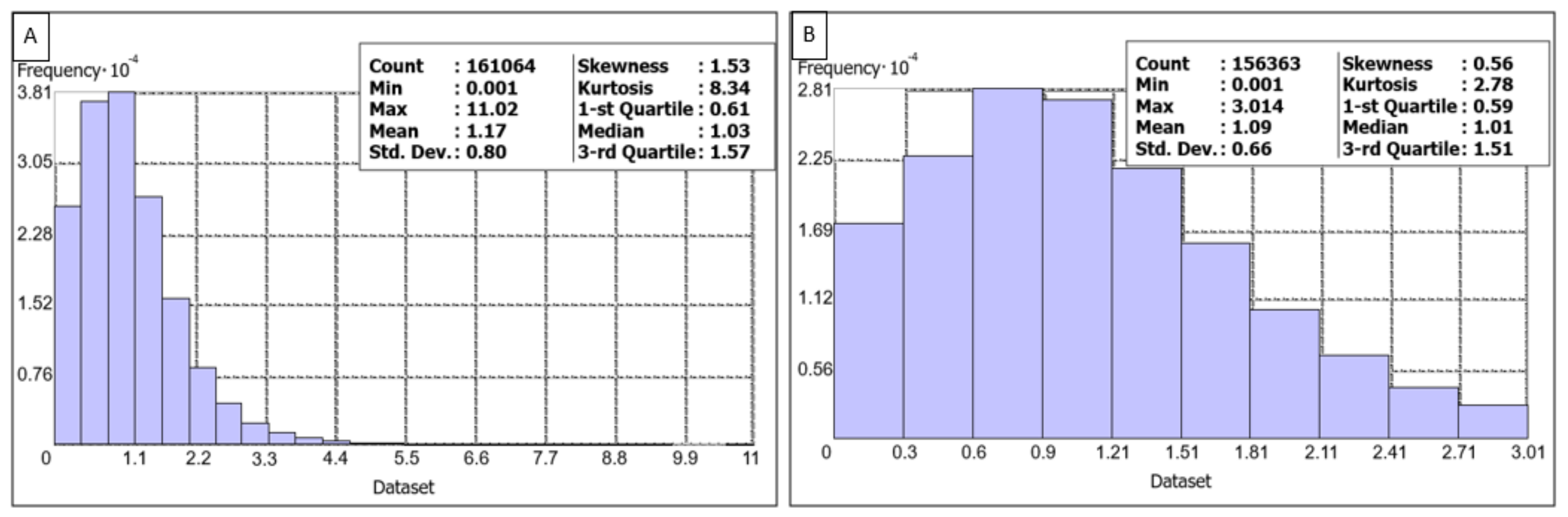
- Define the flood depth distribution
- Flood volume calculation
4. Result and Discussion
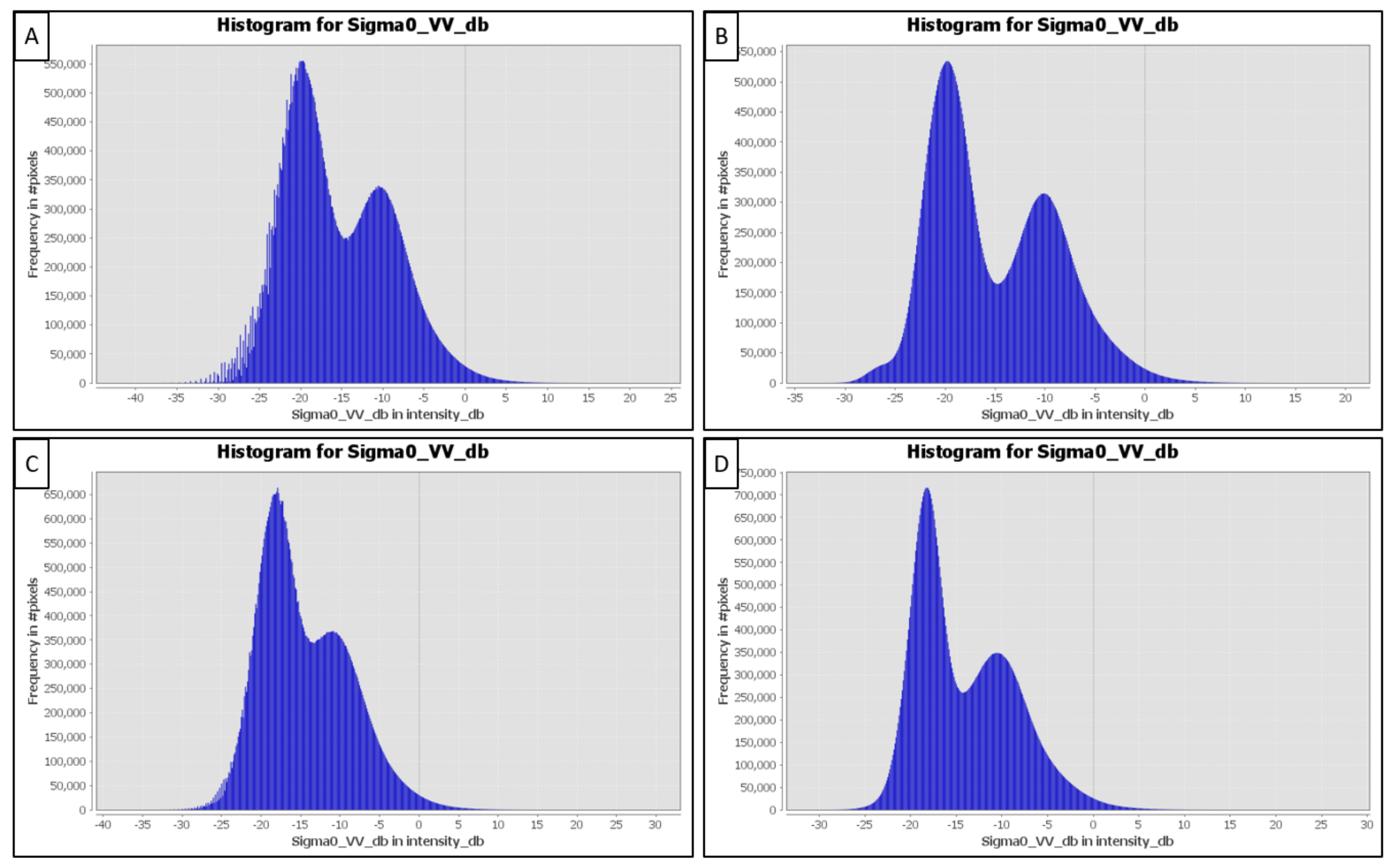
4.1. Selecting Representative dB Value from Crisis Image
- The flat sand morphology will be detected as water because it has similar backscatter data.
- There is almost no permanent river or lake; therefore, the condition before the flood occurred is dry. Water content inside the soil will cause stronger backscattering because the SAR signal penetration ability will become stronger than dryer sand. Due to this reason, the backscatter during rainy conditions will tend to increase [50].
4.2. Flood Surface Interpolation
4.3. Flood Depth Distribution
4.4. Flood Volume Quantification
5. Conclusions
Author Contributions
Funding
Data Availability Statement
Conflicts of Interest
References
- Hu, M.; Zhang, X.; Li, Y.; Yang, H.; Tanaka, K. Flood mitigation performance of low impact development technologies under different storms for retrofitting an urbanized area. J. Clean. Prod. 2019, 222, 373–380. [Google Scholar] [CrossRef]
- Jha, A.K.; Bloch, R.; Lamond, J. Cities and Flooding: A Guide to Integrated Urban Flood Risk Management for the 21st Century; The World Bank: Washington, DC, USA, 2012. [Google Scholar]
- Martinis, S. Improving flood mapping in arid areas using SENTINEL-1 time series data. In Proceedings of the 2017 IEEE International Geoscience and Remote Sensing Symposium (IGARSS), Fort Worth, TX, USA, 23–28 July 2017; pp. 193–196. [Google Scholar]
- Malguzzi, P.; Grossi, G.; Buzzi, A.; Ranzi, R.; Buizza, R. The 1966 “century” flood in Italy: A meteorological and hydrological revisitation. J. Geophys. Res. Atmos. 2006, 111. [Google Scholar] [CrossRef]
- Budiman, J.S.; Al-Amri, N.S.; Chaabani, A.; Elfeki, A.M. Geostatistical based framework for spatial modeling of groundwater level during dry and wet seasons in an arid region: A case study at Hadat Ash-Sham experimental station, Saudi Arabia. Stoch. Environ. Res. Risk Assess. 2021, 1–15. [Google Scholar] [CrossRef]
- Aldhebiani, A.Y.; Elhag, M.; Hegazy, A.K.; Galal, H.K.; Mufareh, N.S. Consideration of NDVI thematic changes in density analysis and floristic composition of Wadi Yalamlam, Saudi Arabia. Geosci. Instrum. Methods Data Syst. 2018, 7, 297–306. [Google Scholar] [CrossRef] [Green Version]
- Hooke, J.M. Extreme sediment fluxes in a dryland flash flood. Sci. Rep. 2019, 9, 1–12. [Google Scholar] [CrossRef] [PubMed]
- Alharthi, A.; El-Sheikh, M.A.; Elhag, M.; Alatar, A.A.; Abbadi, G.A.; Abdel-Salam, E.M.; Arif, I.A.; Baeshen, A.A.; Eid, E.M. Remote sensing of 10 years changes in the vegetation cover of the northwestern coastal land of Red Sea, Saudi Arabia. Saudi J. Biol. Sci. 2020, 27, 3169–3179. [Google Scholar] [CrossRef] [PubMed]
- Derdour, A.; Bouanani, A.; Babahamed, K. Modelling rainfall runoff relations using HEC-HMS in a semi-arid region: Case study in Ain Sefra watershed, Ksour Mountains (SW Algeria). J. Water Land Dev. 2018, 36, 45–55. [Google Scholar] [CrossRef] [Green Version]
- El Alfy, M. Assessing the impact of arid area urbanization on flash floods using GIS, remote sensing, and HEC-HMS rainfall–runoff modeling. Hydrol. Res. 2016, 47, 1142–1160. [Google Scholar] [CrossRef] [Green Version]
- Yang, J.-L.; Zhang, G.-L. Water infiltration in urban soils and its effects on the quantity and quality of runoff. J. Soils Sediments 2011, 11, 751–761. [Google Scholar] [CrossRef]
- Dano, U.L. Flash Flood Impact Assessment in Jeddah City: An Analytic Hierarchy Process Approach. Hydrol. 2020, 7, 10. [Google Scholar] [CrossRef] [Green Version]
- Elfeki, A.; Masoud, M.; Niyazi, B. Integrated rainfall–runoff and flood inundation modeling for flash flood risk assessment under data scarcity in arid regions: Wadi Fatimah basin case study, Saudi Arabia. Nat. Hazards 2017, 85, 87–109. [Google Scholar] [CrossRef]
- Subyani, A.M. Hydrologic behavior and flood probability for selected arid basins in Makkah area, western Saudi Arabia. Arab. J. Geosci. 2009, 4, 817–824. [Google Scholar] [CrossRef]
- Alamri, Y.A. Rains and floods in Saudi Arabia. Crying of the sky or of the people? Saudi Med. J. 2011, 32, 311–313. [Google Scholar]
- Elhag, M.; Bahrawi, J.A. Deterioration of shallow costal environments using synthetic aperture radar data. Desalin. Water Treat. 2020, 194, 333–342. [Google Scholar] [CrossRef]
- Bahrawi, J.; Ewea, H.; Kamis, A.; Elhag, M. Potential flood risk due to urbanization expansion in arid environments, Saudi Arabia. Nat. Hazards 2020, 104, 795–809. [Google Scholar] [CrossRef]
- Li, G.-F.; Xiang, X.-Y.; Tong, Y.-Y.; Wang, H.-M. Impact assessment of urbanization on flood risk in the Yangtze River Delta. Stoch. Environ. Res. Risk Assess. 2013, 27, 1683–1693. [Google Scholar] [CrossRef]
- Mahmoud, S.H.; Gan, T.Y. Urbanization and climate change implications in flood risk management: Developing an efficient decision support system for flood susceptibility mapping. Sci. Total. Environ. 2018, 636, 152–167. [Google Scholar] [CrossRef]
- Mirza, M.M.Q. Climate change, flooding in South Asia and implications. Reg. Environ. Change 2010, 11, 95–107. [Google Scholar] [CrossRef]
- Schlaffer, S.; Chini, M.; Giustarini, L.; Matgen, P. Probabilistic mapping of flood-induced backscatter changes in SAR time series. Int. J. Appl. Earth Obs. Geoinf. 2017, 56, 77–87. [Google Scholar] [CrossRef]
- Bajabaa, S.; Masoud, M.; Al-Amri, N. Flash flood hazard mapping based on quantitative hydrology, geomorphology and GIS techniques (case study of Wadi Al Lith, Saudi Arabia). Arab. J. Geosci. 2014, 7, 2469–2481. [Google Scholar] [CrossRef]
- Elkarim, A.; Awawdeh, M.; Alogayell, H.; Al-Alola, S. Intergration Remote Sensing and Hydrologic, Hydroulic Modelling on Assessment Flood Risk and Mitigation: Al-Lith City, KSA. Int. J. GEOMATE 2020, 18, 252–280. [Google Scholar] [CrossRef]
- Jones, H.G.; Vaughan, R.A. Remote Sensing of Vegetation: Principles, Techniques, and Applications; Oxford University Press: Oxford, UK, 2010. [Google Scholar]
- Price, J. Using spatial context in satellite data to infer regional scale evapotranspiration. IEEE Trans. Geosci. Remote. Sens. 1990, 28, 940–948. [Google Scholar] [CrossRef] [Green Version]
- Dong, Z.; Wang, Z.; Liu, D.; Song, K.; Li, L.; Jia, M.; Ding, Z. Mapping Wetland Areas Using Landsat-Derived NDVI and LSWI: A Case Study of West Songnen Plain, Northeast China. J. Indian Soc. Remote. Sens. 2014, 42, 569–576. [Google Scholar] [CrossRef]
- Ghasemigoudarzi, P.; Huang, W.; De Silva, O.; Yan, Q.; Power, D. A Machine Learning Method for Inland Water Detection Using CYGNSS Data. IEEE Geosci. Remote. Sens. Lett. 2020, 1–5. [Google Scholar] [CrossRef]
- Ghasemigoudarzi, P.; Huang, W.; De Silva, O.; Yan, Q.; Power, D.T. Flash Flood Detection from CYGNSS Data Using the RUSBoost Algorithm. IEEE Access 2020, 8, 171864–171881. [Google Scholar] [CrossRef]
- Imam, R.; Pini, M.; Marucco, G.; Dominici, F.; Dovis, F. UAV-Based GNSS-R for Water Detection as a Support to Flood Moni-toring Operations: A Feasibility Study. Appl. Sci. 2020, 10, 210. [Google Scholar] [CrossRef] [Green Version]
- Kouassi, K.H.; N’go, Y.A.; Anoh, K.A.; Koua, T.J.-J.; Stoleriu, C.C. Contribution of Sentinel 1 Radar Data to Flood Mapping in the San-Pédro River Basin (South-west Côte d’Ivoire). Asian J. Geogr. Res. 2020, 3, 1–8. [Google Scholar] [CrossRef] [Green Version]
- Tavus, B.; Kocaman, S.; Gokceoglu, C.; Nefeslioglu, H.A. Considerations on the Use of Sentinel-1 Data in Flood Mapping in Urban Areas: Ankara (Turkey) 2018 Floods. ISPRS Int. Arch. Photogramm. Remote. Sens. Spat. Inf. Sci. 2018, XLII-5, 575–581. [Google Scholar] [CrossRef] [Green Version]
- Twele, A.; Cao, W.; Plank, S.; Martinis, S. Sentinel-1-based flood mapping: A fully automated processing chain. Int. J. Remote Sens. 2016, 37, 2990–3004. [Google Scholar] [CrossRef]
- Elhag, M.; Abdurahman, S.G. Advanced remote sensing techniques in flash flood delineation in Tabuk City, Saudi Arabia. Nat. Hazards 2020, 103, 3401–3413. [Google Scholar] [CrossRef]
- Cham, T.; Mitani, Y.; Fujii, K.; Ikemi, H. Evaluation of flood volume and inundation depth by GIS midstream of Chao Phra-ya River Basin, Thailand. WIT Trans. Built Environ. 2015, 168, 1049–1060. [Google Scholar]
- Cohen, S.; Brakenridge, G.R.; Kettner, A.; Bates, B.; Nelson, J.; McDonald, R.; Huang, Y.F.; Munasinghe, D.; Zhang, J. Estimat-ing floodwater depths from flood inundation maps and topography. JAWRA J. Am. Water Resour. Assoc. 2018, 54, 847–858. [Google Scholar] [CrossRef]
- Elhag, M.; Galal, H.K.; Alsubaie, H. Understanding of morphometric features for adequate water resource management in arid environments. Geosci. Instrum. Methods Data Syst. 2017, 6, 293–300. [Google Scholar] [CrossRef] [Green Version]
- Schumm, S.A. Evolution of Drainage Systems and Slopes in Badlands at Perth Amboy, New Jersey. GSA Bull. 1956, 67, 597–646. [Google Scholar] [CrossRef]
- Horton, R.E. Erosional development of streams and their drainage basins; hydrophysical approach to quantitative morphology. GSA Bull. 1945, 56, 275–370. [Google Scholar] [CrossRef] [Green Version]
- Albishi, M.; Bahrawi, J.; Elfeki, A. Derivation of the unit hydrograph of Allith Basin in the South West of Saudi Arabia. Int J. Water Res. Environ. 2017, 6, 50–57. [Google Scholar]
- Bahrawi, J.A.; Elhag, M.; Aldhebiani, A.Y.; Galal, H.K.; Hegazy, A.K.; Alghailani, E. Soil Erosion Estimation Using Remote Sensing Techniques in Wadi Yalamlam Basin, Saudi Arabia. Adv. Mater. Sci. Eng. 2016, 2016, 9585962. [Google Scholar] [CrossRef] [Green Version]
- Kyriou, A.; Nikolakopoulos, K. Flood mapping from Sentinel-1 and Landsat-8 data: A case study from river Evros, Greece. In Proceedings of the Earth Resources and Environmental Remote Sensing/GIS Applications VI, Toulouse, France, 22–24 September 2015; p. 964405. [Google Scholar]
- Zotou, I.; Bellos, V.; Gkouma, A.; Karathanassi, V.; Tsihrintzis, V.A. Using Sentinel-1 imagery to assess predictive performance of a hydraulic model. Water Res. Manag. 2020, 34, 4415–4430. [Google Scholar] [CrossRef]
- Elhag, M.; Yimaz, N.; Bahrawi, J.; Boteva, S. Evaluation of Optical Remote Sensing Data in Burned Areas Mapping of Thasos Island, Greece. Earth Syst. Environ. 2020, 4, 813–826. [Google Scholar] [CrossRef]
- Clement, M.; Kilsby, C.; Moore, P. Multi-temporal synthetic aperture radar flood mapping using change detection. J. Flood Risk Manag. 2018, 11, 152–168. [Google Scholar] [CrossRef]
- Henry, J.; Chastanet, P.; Fellah, K.; Desnos, Y. Envisat multi-polarized ASAR data for flood mapping. Int. J. Remote Sens. 2006, 27, 1921–1929. [Google Scholar] [CrossRef]
- Elhag, M.; Yilmaz, N. Insights of remote sensing data to surmount rainfall/runoff data limitations of the downstream catchment of Pineios River, Greece. Environ. Earth Sci. 2021, 80, 35. [Google Scholar] [CrossRef]
- Lee, J.-S.; Wen, J.-H.; Ainsworth, T.L.; Chen, K.-S.; Chen, A.J. Improved Sigma Filter for Speckle Filtering of SAR Imagery. IEEE Trans. Geosci. Remote Sens. 2009, 47, 202–213. [Google Scholar] [CrossRef]
- Conde, F.C.; Muñoz, M.D.M. Flood Monitoring Based on the Study of Sentinel-1 SAR Images: The Ebro River Case Study. Water 2019, 11, 2454. [Google Scholar] [CrossRef] [Green Version]
- Elhag, M.; Bahrawi, J.A. Sedimentation mapping in shallow shoreline of arid environments using active remote sensing data. Nat. Hazards 2019, 99, 879–894. [Google Scholar] [CrossRef]
- Ridley, J.; Strawbridge, F.; Card, R.; Phillips, H. Radar backscatter characteristics of a desert surface. Remote. Sens Environ. 1996, 57, 63–78. [Google Scholar] [CrossRef]
- Vinutha, H.P.; Poornima, B.; Sagar, B.M. Detection of Outliers Using Interquartile Range Technique from Intrusion Dataset. In Information and Decision Sciences; Springer: Berlin, Germany, 2018; pp. 511–518. [Google Scholar]
- Farran, M.M.; Elfeki, A.; Elhag, M.; Chaabani, A. A comparative study of the estimation methods for NRCS curve number of natural arid basins and the impact on flash flood predications. Arab. J. Geosci. 2021, 14, 1–23. [Google Scholar] [CrossRef]
- Ewea, H.A.; Al-Amri, N.S.; Elfeki, A.M. Analysis of maximum flood records in the arid environment of Saudi Arabia. Geomat. Nat. Hazards Risk 2020, 11, 1743–1759. [Google Scholar] [CrossRef]
- Hsu, K.-L.; Gao, X.; Sorooshian, S.; Gupta, H.V. Precipitation Estimation from Remotely Sensed Information Using Artificial Neural Networks. J. Appl. Meteorol. 1997, 36, 1176–1190. [Google Scholar] [CrossRef]


Publisher’s Note: MDPI stays neutral with regard to jurisdictional claims in published maps and institutional affiliations. |
© 2021 by the authors. Licensee MDPI, Basel, Switzerland. This article is an open access article distributed under the terms and conditions of the Creative Commons Attribution (CC BY) license (https://creativecommons.org/licenses/by/4.0/).
Share and Cite
Budiman, J.; Bahrawi, J.; Hidayatulloh, A.; Almazroui, M.; Elhag, M. Volumetric Quantification of Flash Flood Using Microwave Data on a Watershed Scale in Arid Environments, Saudi Arabia. Sustainability 2021, 13, 4115. https://doi.org/10.3390/su13084115
Budiman J, Bahrawi J, Hidayatulloh A, Almazroui M, Elhag M. Volumetric Quantification of Flash Flood Using Microwave Data on a Watershed Scale in Arid Environments, Saudi Arabia. Sustainability. 2021; 13(8):4115. https://doi.org/10.3390/su13084115
Chicago/Turabian StyleBudiman, Jaka, Jarbou Bahrawi, Asep Hidayatulloh, Mansour Almazroui, and Mohamed Elhag. 2021. "Volumetric Quantification of Flash Flood Using Microwave Data on a Watershed Scale in Arid Environments, Saudi Arabia" Sustainability 13, no. 8: 4115. https://doi.org/10.3390/su13084115