
A Detailed Forecast of the Technologies Based on Lifecycle Analysis of GMAW and CMT Welding Processes

 ,
,  ,
,
Abstract
:
1. Introduction
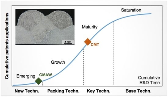
2. The TLC Approach Based on the S-Curve Concept
3. Materials and Methods
3.1. The Welding Analyses
3.1.1. Sample Preparation
3.1.2. Temperature Measurements
3.1.3. Welding Characterisation
3.2. TLC Analyses of Technological Maturity
3.2.1. Data Collection and Preparation
- GMAW technology: AB = ((gmaw OR (gas ADJ metal ADJ arc ADJ welding)) AND welding) OR AB = ((mag OR (metal ADJ active ADJ gas)) AND welding) OR AB = ((mig OR (metal ADJ inert ADJ gas)) AND welding) NOT AB = ((cold ADJ metal ADJ transfer)) NOT AB = (cmt);
- CMT technology: AB = ((cold ADJ metal ADJ transfer)) OR AB = ((cmt)) AND AB = (welding) NOT AB = ((mag OR (metal ADJ active ADJ gas))) NOT AB = ((mig OR (metal ADJ inert ADJ gas))).
3.2.2. Statistical Model Development and Tests
- Time-series: The forecast (8.11) package developed by Hyndman et al. [37], which contains methods for smoothing and forecasting using time-series analysis and linear models;
- Growth-curves: The growthrates (0.8.1) package developed by Petzoldt [38], which includes nonlinear growth models with varying quantities of parameters written as analytical solutions of the differential equation.
3.2.3. Analyses and Comparisons between the Models
4. Results and Discussion
4.1. Welding Analyses
4.2. TLC Analyses and Assessment of Technological Maturity
4.2.1. The Dataset Characteristics
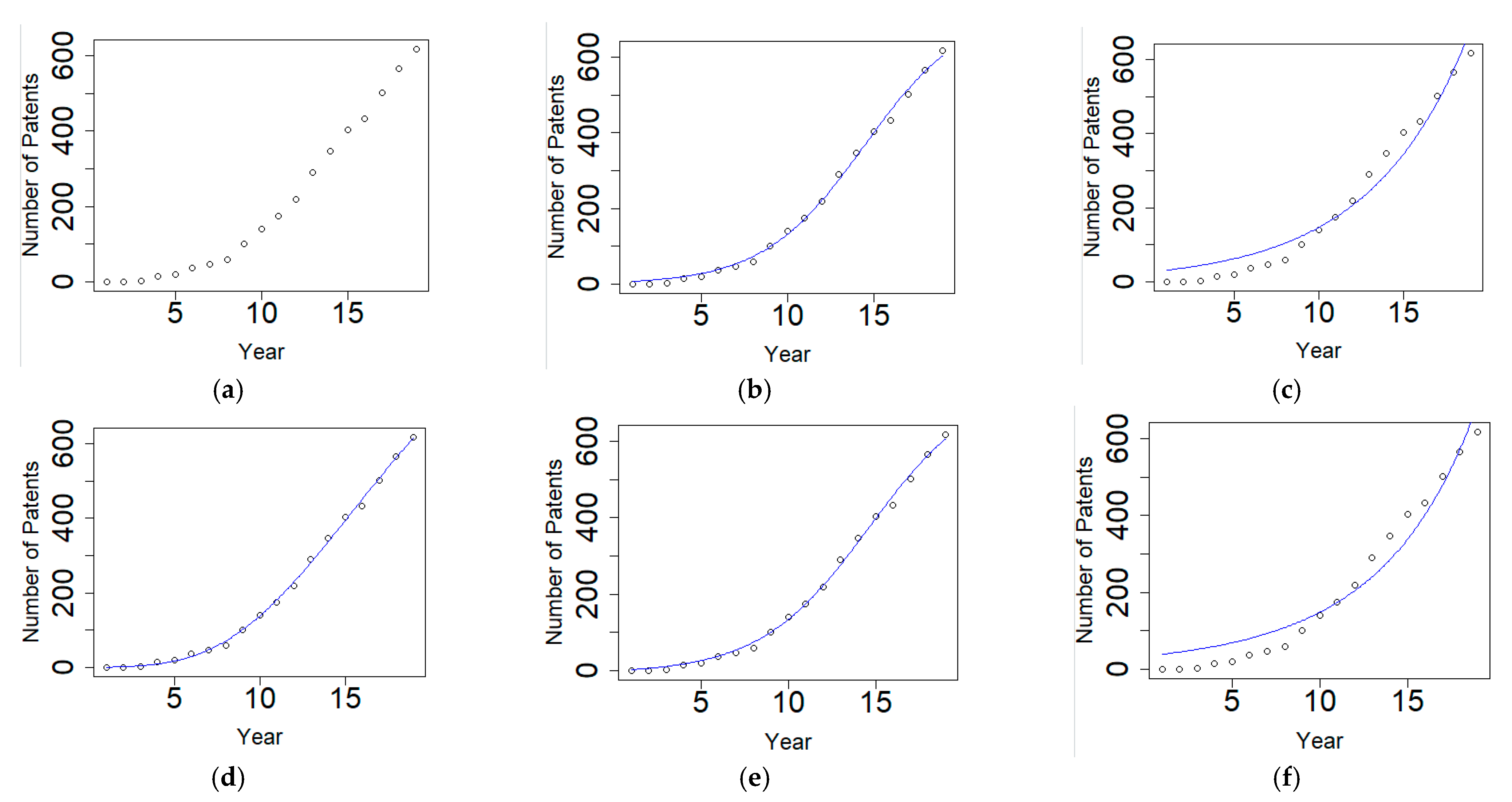
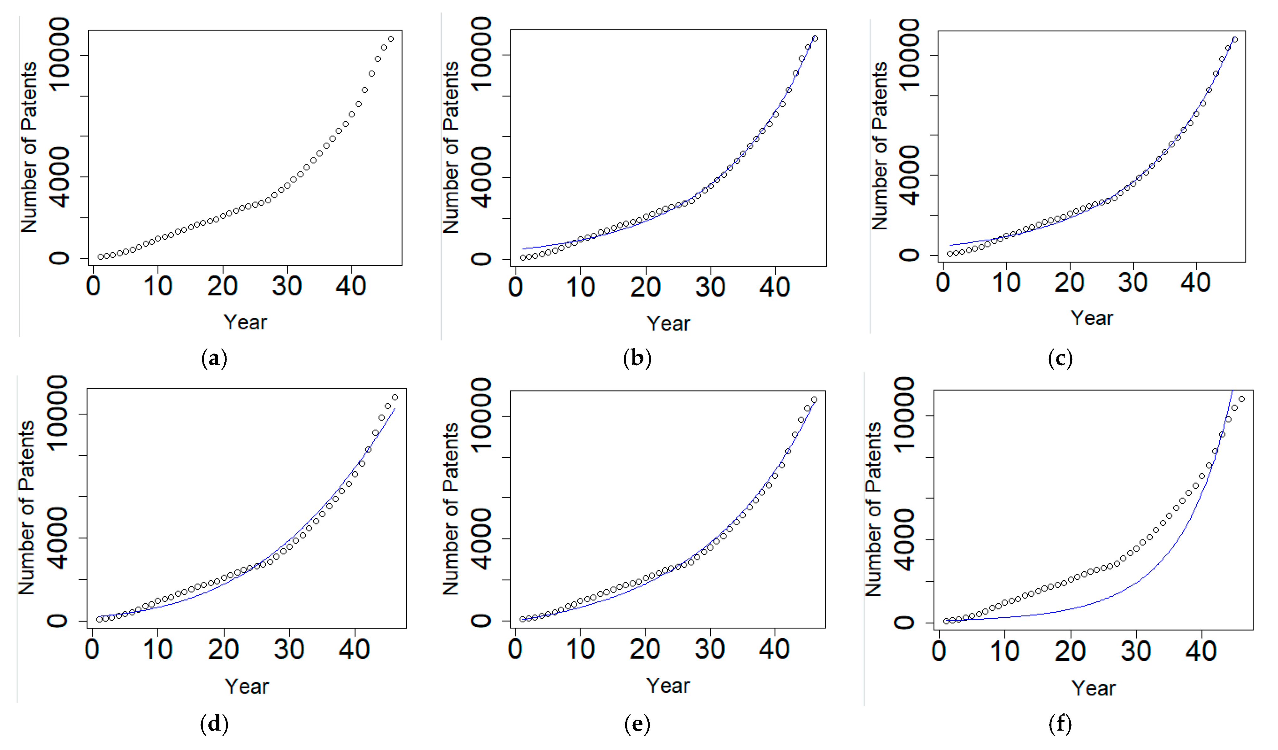
4.2.2. Development of TLC Models and Analyses
CMT Technology
Using the Best Models to Forecast
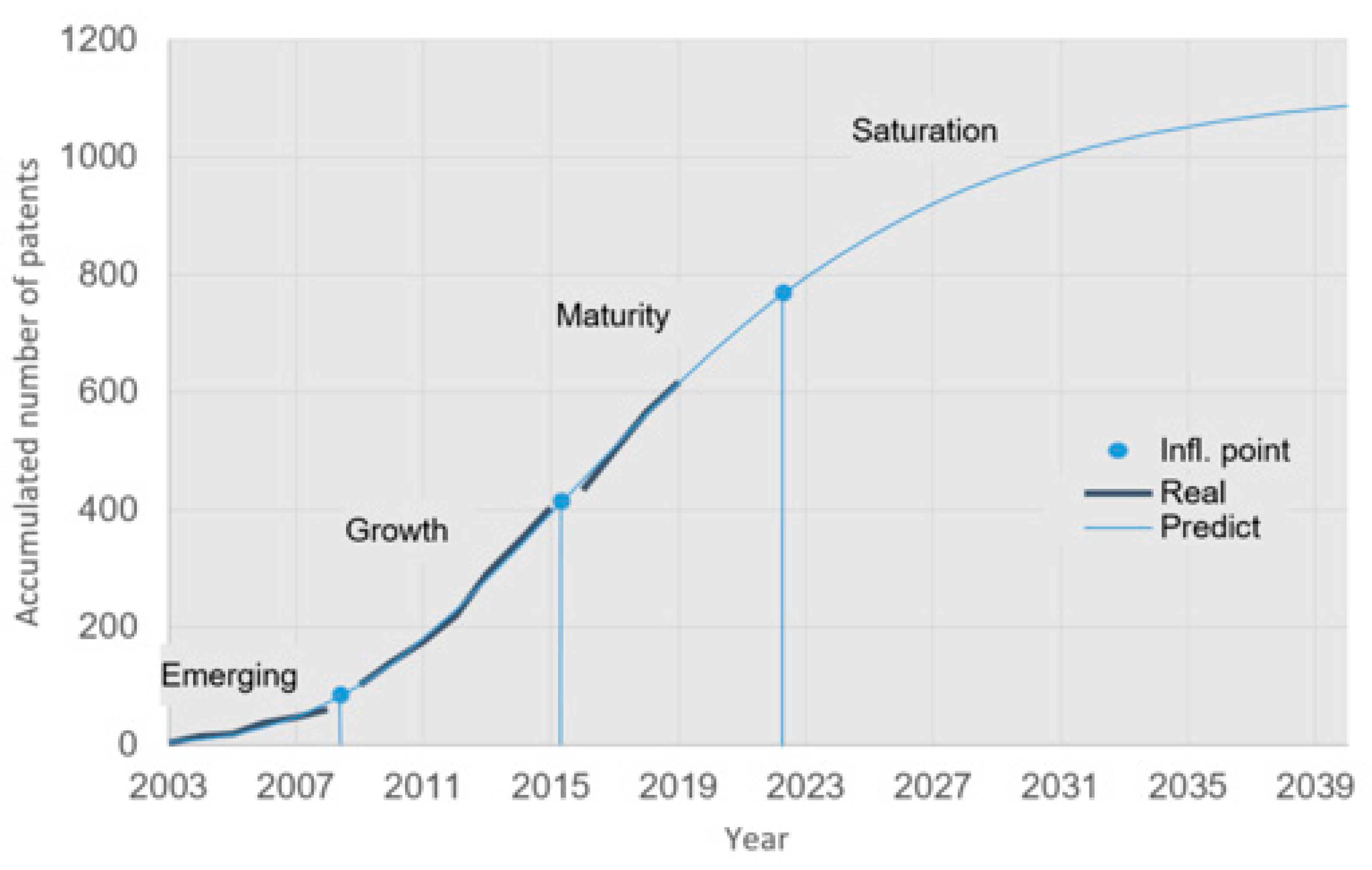
Establishing the Curve and Its Inflection Points
- Let f be a derivative function up to 2nd order in the interval I and suppose that at x0 ∈ I, f″(x0) <> 0. In this case, if f″(x0) > 0, then the curve of f has a positive concavity in x0; otherwise, the curve of f″(x0) > 0 has a negative concavity in x0;
- Let f be a derivative function up to 2nd order in an interval I and suppose that x0 ∈ I is the abscissa of an inflection point in the curve of f. Thus, f″(x0) = 0.
GMAW Technology
Using the Best Models to Forecast
Establishing the Curve and Its Inflection Points
5. Conclusions
5.1. Welding Characteristics
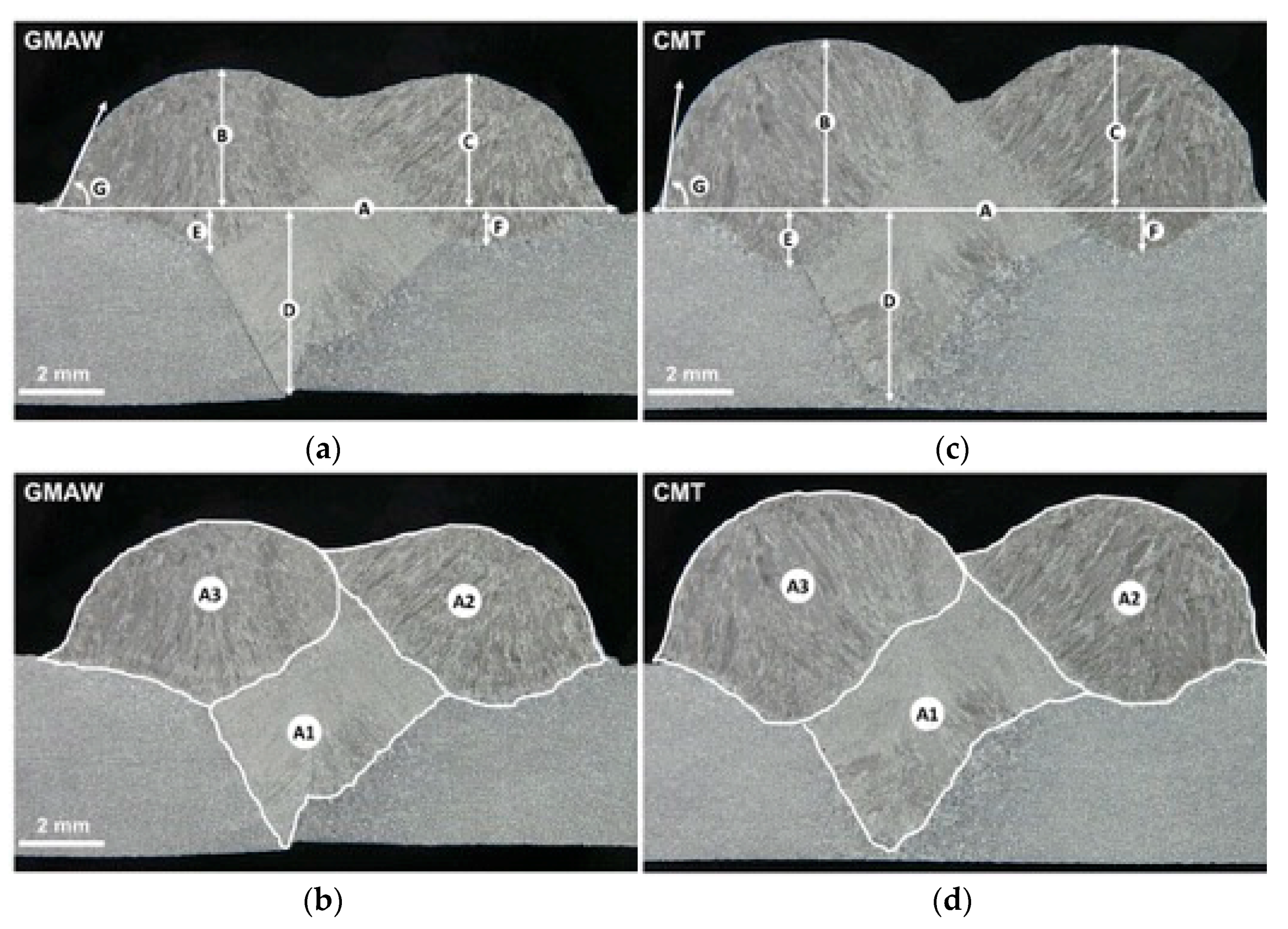
- Visual inspection revealed a good welding bead with a lack of superficial defects and discontinuities for both processes. The chosen parameters ensured similar heat inputs in both prepared joints, and the analyses showed that the CMT process promoted a high deposition rate and less heat transfer to the base material compared to standard GMAW. This supported the lack of penetration and the pronounced welding bead observed for the CMT joints;
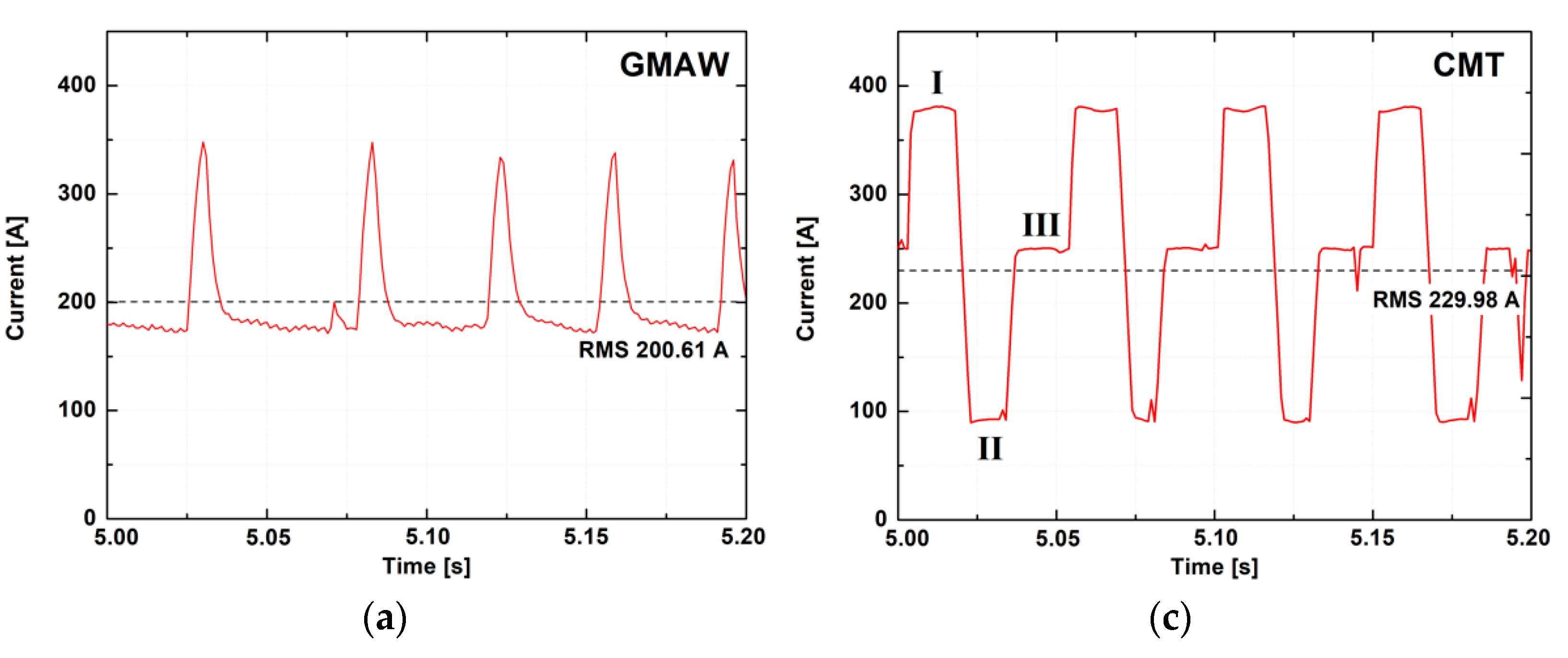
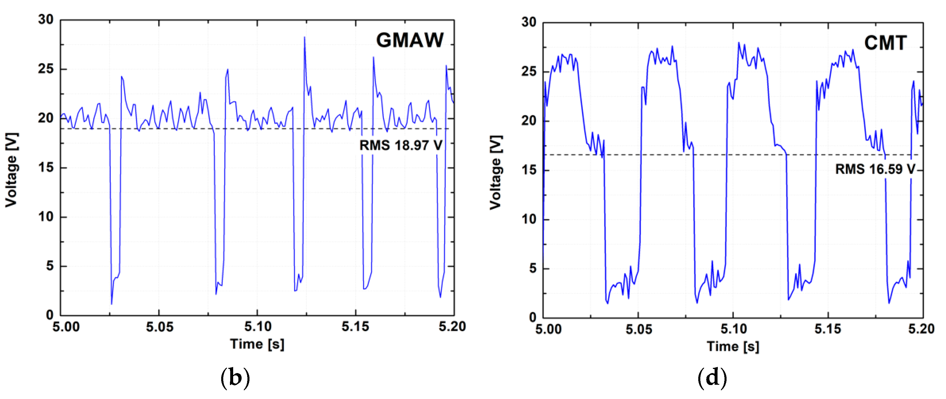
- The short circuit frequency analyses confirmed the stable and controlled material deposition under the CMT process, revealing a distinct frequency for material transfer. The monitored voltage and current parameters revealed the three typical phases connected with peaks of current and arc reignition after the filler material melted. At that moment, a small droplet of molten metal was detached, followed by a voltage reduction;
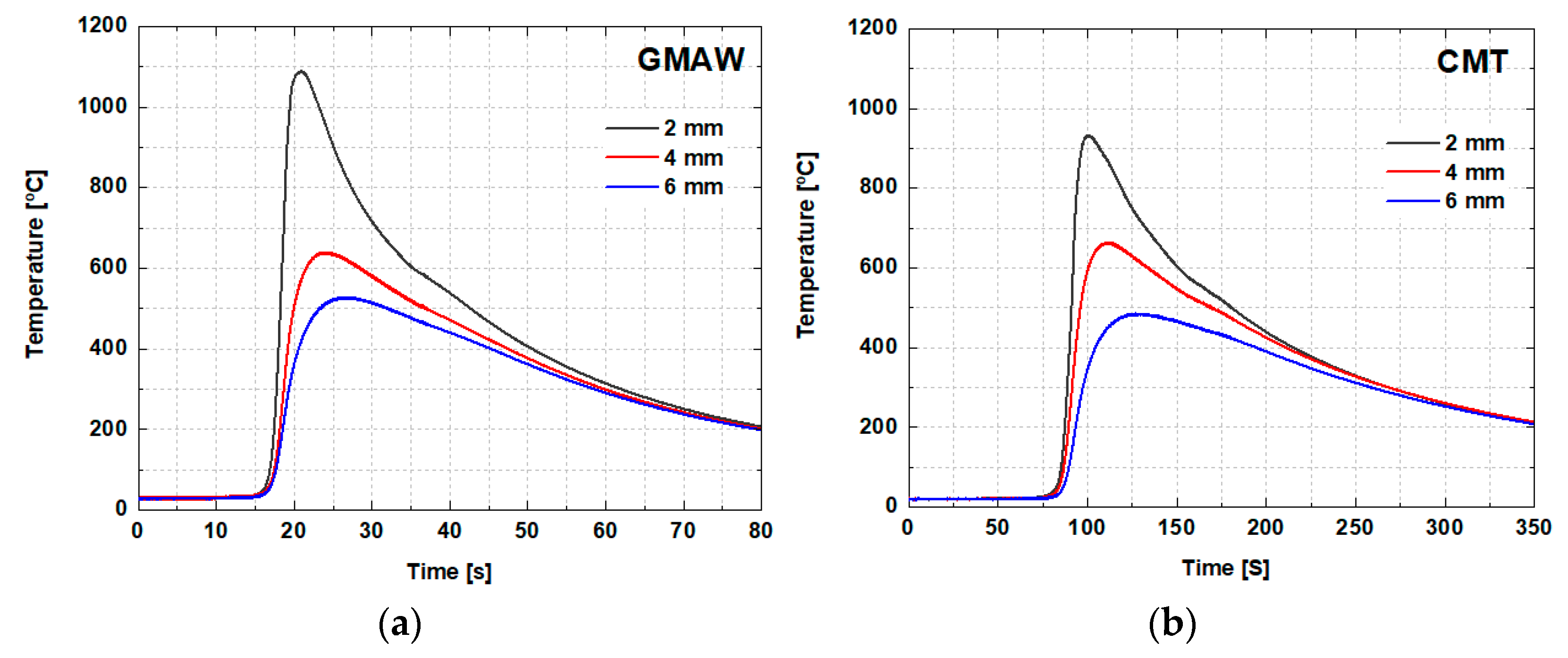
- The monitored temperature profile confirms that the GMAW process promoted high temperature peaks and cooling rates, which led to a high heat transfer to the base material with peaks of current when the arc reignited after the short circuit phase.
5.2. TLC Analyses
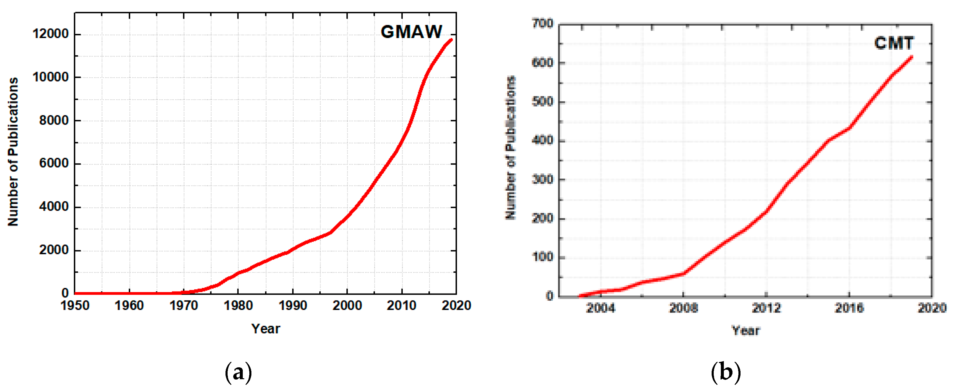
- The patent dataset developed and used in this study revealed that GMAW technology has more than twenty times the number of patents of CMT. This may be connected with the high possibility of adjustment, automation, and time use with this technology. The main clusters of the request themes/topics were related to the methodology, characteristics, and applications. The analyses also revealed that few countries and companies dominate patent deposition in the field of CMT welding technology. This scenario offers a great opportunity for other countries and companies to study and deliver new solutions to the market in this regard.
- The use of advanced models to predict the S-curve trends revealed that, for the CMT process, the formula obtained by Richards growth-curve was the one that best represented the data obtained from the patents. Instead, for the GMAW process, the growth-curve model using the Baranyi methodology was the one that best fit with the original data. Both models differed mainly in their algorithms for inflection points, thus providing a clearer view of the behaviour of the technology and its possible predictions;
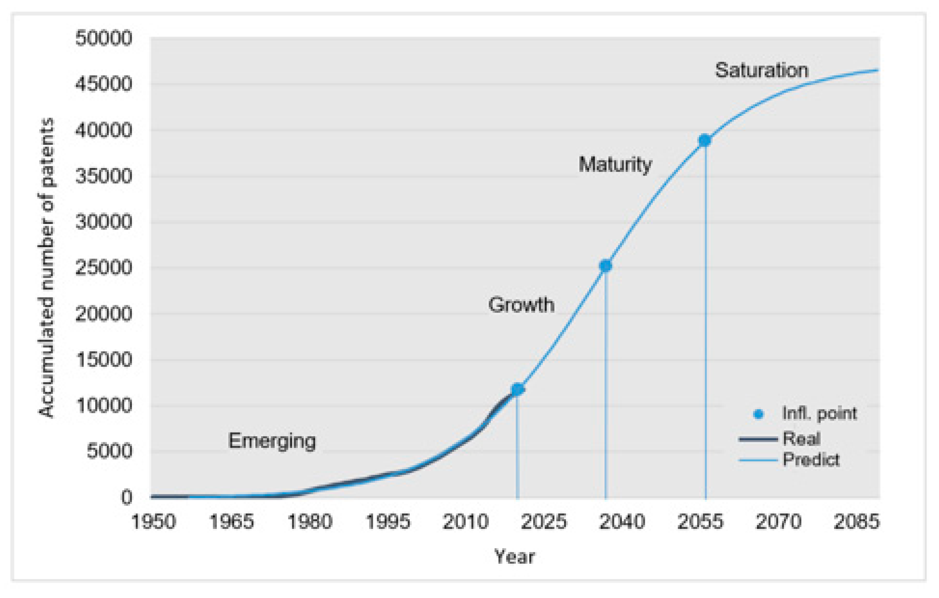
- The S-curve trend for the CMT process revealed that, despite being recent, the technology is already in a mature phase, a fact confirmed by the experts’ opinions due to the limited use of this technology. For the GMAW process, despite being older, this technology is positioned in the growth phase on the S-curve, indicating great possibility for advancement—a fact also supported by the opinions of the experts.
- The results confirm that mathematical modelling can precisely reveal the inflection points and phases of each technology, which provides a new possible perspective of analysis in terms of maturity level. This kind of methodology together with the experts’ opinion can be essential for assisting in the decision-making and analysis of technological trends.
Author Contributions
Funding
Conflicts of Interest
References
- Yapp, D.; Blackman, S.A. Recent Developments in High Productivity Pipeline Welding. J. Braz. Soc. Mech. Sci. Eng. 2004, 26, 89–97. [Google Scholar] [CrossRef] [Green Version]
- Shen, H.; Deng, R.; Liu, B.; Tang, S.; Li, S. Study of the mechanism of a stable deposited height during GMAW-based additive manufacturing. Appl. Sci. 2020, 10, 4322. [Google Scholar] [CrossRef]
- Goede, M.; Stehlin, M.; Rafflenbeul, L.; Kopp, G.; Beeh, E. Super Light Car—Lightweight construction thanks to a multi-material design and function integration. Eur. Transp. Res. Rev. 2009, 1, 5–10. [Google Scholar] [CrossRef] [Green Version]
- Madhavan, S.; Kamaraj, M.; Vijayaraghavan, L. Microstructure and mechanical properties of cold metal transfer welded aluminium/dual phase steel. Sci. Technol. Weld. Join. 2016, 21, 194–200. [Google Scholar] [CrossRef]
- Cornacchia, G.; Cecchel, S.; Panvini, A. A comparative study of mechanical properties of metal inert gas (MIG)-cold metal transfer (CMT) and fiber laser-MIG hybrid welds for 6005A T6 extruded sheet. Int. J. Adv. Manuf. Technol. 2018, 94, 2017–2030. [Google Scholar] [CrossRef]
- Selvi, S.; Vishvaksenan, A.; Rajasekar, E. Cold metal transfer (CMT) technology—An overview. Def. Technol. 2018, 14, 28–44. [Google Scholar] [CrossRef]
- Zhang, H.T.; Feng, J.C.; He, P.; Zhang, B.B.; Chen, J.M.; Wang, L. The arc characteristics and metal transfer behaviour of cold metal transfer and its use in joining aluminium to zinc-coated steel. Mater. Sci. Eng. A 2009, 499, 111–113. [Google Scholar] [CrossRef]
- Pickin, C.G.; Williams, S.W.; Lunt, M. Characterisation of the cold metal transfer (CMT) process and its application for low dilution cladding. J. Mater. Process. Technol. 2011, 211, 496–502. [Google Scholar] [CrossRef] [Green Version]
- Costa, T.F.; Benedetti Filho, E.; Arevalo, H.D.H.; Vilarinho, L.O. Assessment of Conventional and Controlled Short-Circuit MIG/MAG Processes for Steel-Pipe Welding in Single Pass. Soldag. Inspeção 2012, 17, 356–368. [Google Scholar] [CrossRef] [Green Version]
- Chang, Y.J.; Sproesser, G.; Neugebauer, S.; Wolf, K.; Scheumann, R.; Pittner, A.; Rethmeier, M.; Finkbeiner, M. Environmental and Social Life Cycle Assessment of Welding Technologies. Procedia Cirp 2015, 26, 293–298. [Google Scholar] [CrossRef] [Green Version]
- Taylor, M.; Taylor, A. The technology life cycle: Conceptualization and managerial implications. Int. J. Prod. Econ. 2012, 140, 541–553. [Google Scholar] [CrossRef]
- Wilder, J.; Sossa, Z.; Palop, F.; Alzate, B.A.; Mauricio, F.; Salazar, V.; Felipe, A.; Patiño, A. S-Curve Analysis and the Technology Life Cycle: Application in Series of Data of Articles and Patents. Espacios 2016, 37, 19. [Google Scholar]
- Little, A.D. The strategic management of technology. Eur. Manag. Forums 1981, 1, 1–39. [Google Scholar]
- Wu, J.; Yang, Z.; Hu, X.; Wang, H.; Huang, J. Exploring driving forces of sustainable development of China’s new energy vehicle industry: An analysis from the perspective of an innovation ecosystem. Sustainability 2018, 10, 4827. [Google Scholar] [CrossRef] [Green Version]
- Gao, L.; Porter, A.L.; Wang, J.; Fang, S.; Zhang, X.; Ma, T.; Wang, W.; Huang, L. Technology life cycle analysis method based on patent documents. Technol. Forecast. Soc. Chang. 2013, 80, 398–407. [Google Scholar] [CrossRef]
- Xin’an, W.; Aijun, M. Comparison of four nonlinear growth models for effective exploration of growth characteristics of turbot Scophthalmus maximus fish strain. Afr. J. Biotechnol. 2016, 15, 2251–2258. [Google Scholar] [CrossRef] [Green Version]
- Madvar, M.D.; Khosropour, H.; Khosravanian, A.; Mirafshar, M.; Azaribeni, A.; Rezapour, M.; Nouri, B. Patent-based technology life cycle analysis: The case of the petroleum industry. Foresight STI Gov. 2016, 10, 72–79. [Google Scholar] [CrossRef]
- Jamali, M.Y.; Aslani, A.; Moghadam, B.F.; Naaranoja, M.; Madvar, M.D. Analysis of photovoltaic technology development based on technology life cycle approach. J. Renew. Sustain. Energy 2016, 8. [Google Scholar] [CrossRef]
- Fye, S.R.; Charbonneau, S.M.; Hay, J.W.; Mullins, C.A. An examination of factors affecting accuracy in technology forecasts. Technol. Forecast. Soc. Chang. 2013, 80, 1222–1231. [Google Scholar] [CrossRef]
- Smith, M.; Agrawal, R. A Comparison of Time Series Model Forecasting Methods on Patent Groups. In Proceedings of the CEUR Workshop Proceedings, Rome, Italy, 24–25 November 2014; pp. 167–173. [Google Scholar]
- Andrade, H.; Junior Chagas, M.; Silva, M.; Brito, M.A.; Rocha, D.; Ribeiro, J. Avaliação da Maturidade Tecnológica: Conceitos; Fbra, E.B.E., Ed.; Edição: Jundiaí, Brazil, 2019; ISBN 9786551040009. [Google Scholar]
- Yang, X.; Yu, X.; Liu, X. Obtaining a sustainable competitive advantage from patent information: A patent analysis of the graphene industry. Sustainability 2018, 10, 4800. [Google Scholar] [CrossRef] [Green Version]
- Kucharavy, D.; De Guio, R. Logistic substitution model and technological forecasting. Procedia Eng. 2011, 9, 402–416. [Google Scholar] [CrossRef] [Green Version]
- De Gooijer, J.G.; Hyndman, R.J. 25 Years of Time Series Forecasting. Int. J. Forecast. 2006, 22, 443–473. [Google Scholar] [CrossRef] [Green Version]
- Krispin, R. Hands-On Time Series Analysis with R: Perform Time Series Analysis and Forecasting Using R, 1st ed.; Shetty, S., Ed.; Packt Publishing: Birmingham, UK, 2019; ISBN 9781788629157. [Google Scholar]
- Bouzada, M.A.C. Aprendendo Decomposição Clássica: Tutorial para um Método de Análise de Séries Temporais. TAC Tecnol. Adm. Contab. 2012, 2, 1–18. [Google Scholar] [CrossRef]
- Kabacoff, R.I. R in Action Data Analysis and Graphics with R; Manning Publications: New York, NY, USA, 2011; ISBN 9781935182399. [Google Scholar]
- Lobacz, A.; Kowalik, J.; Tarczynska, A. Modeling the growth of Listeria monocytogenes in mold-ripened cheeses. J. Dairy Sci. 2013, 96, 3449–3460. [Google Scholar] [CrossRef] [PubMed]
- Lezama-Nicolás, R.; Rodríguez-Salvador, M.; Río-Belver, R.; Bildosola, I. A bibliometric method for assessing technological maturity: The case of additive manufacturing. Scientometrics 2018, 117, 1425–1452. [Google Scholar] [CrossRef] [PubMed] [Green Version]
- En, D. Hot Rolled Products of Structural Steels Part 2: Technical Delivery Conditions for Non-Alloy Structural Steels; DIN EN 10025-2; BSI: London, UK, 2005. [Google Scholar]
- Haelsig, A.; Mayr, P.; Kusch, M. Determination of energy flows for welding processes. Weld. World 2016, 60, 259–266. [Google Scholar] [CrossRef]
- Pepe, N.; Egerland, S.; Colegrove, P.A.; Yapp, D.; Leonhartsberger, A.; Scotti, A. Measuring the process efficiency of controlled gas metal arc welding processes. Sci. Technol. Weld. Join. 2011, 16, 412–417. [Google Scholar] [CrossRef] [Green Version]
- Imoudu, N.E.; Ayele, Y.Z.; Barabadi, A. The characteristic of cold metal transfer (CMT) and its application for cladding. In Proceedings of the IEEE International Conference on Industrial Engineering and Engineering Management, the Arctic University of Norway, Bangkok, Thailand, 16–19 December 2018; Volume 2017-Decem, pp. 1883–1887. [Google Scholar]
- Tomków, J.; Czupry´nski, A.; Czupry´nski, C.; Fydrych, D. The Abrasive Wear Resistance of Coatings Manufactured on High-Strength Low-Alloy (HSLA) Offshore Steel in Wet Welding Conditions. Coatings 2020, 10, 219. [Google Scholar] [CrossRef] [Green Version]
- WIPO. WIPO Guide to Using PATENT; WIPO Publishing: New York, NY, USA, 2015; pp. 1–43. [Google Scholar]
- RStudio Team. RStudio: Integrated Development Environment for R. Available online: https://rstudio.com/products/rstudio/ (accessed on 10 March 2019).
- Hyndman, R.; Athanasopoulos, G.; Bergmeir, C.; Caceres, G.; Chhay, L.; O’Hara-Wild, M.; Petropoulos, F.; Razbash, S.; Wang, E.; Yasmeen, F. Forecast: Forecasting Functions for Time Series and LInear Models. Available online: http://pkg.robjhyndman.com/forecast%3E (accessed on 10 March 2020).
- Petzoldt, T. Growthrates: Estimate Growth Rates from Experimental Data; R Package: Auckland City, New Zealand, 2019; p. 42. [Google Scholar]
- Anderson, E.C.; Winter, D.J. Forecasting Functions for Time Series and Linear Models. 2020, p. 140. Available online: https://rstudio.com/products/rstudio/ (accessed on 10 March 2020).
- Kucharavy, D.; De Guio, R. Application of logistic growth curve. Procedia Eng. 2015, 131, 280–290. [Google Scholar] [CrossRef] [Green Version]
- Conservation, P. Growth II—A Major Upgrade to Our “Simply Growth” Software. Fits and Plots von Bertalanffy, Gompertz, Logistic and a Wide Range of Other Growth Curves to Length and/or Weight at Age Data; Pisces Conservation Ltd.: Hampshire, UK, 2006. [Google Scholar]
- Yilmaz, M.T. Identifiability of Baranyi model and comparison with empirical models in predicting effect of essential oils on growth of Salmonella typhimurium in rainbow trout stored under aerobic, modified atmosphere and vacuum packed conditions. Afr. J. Biotechnol. 2011, 10, 7468–7479. [Google Scholar] [CrossRef]
- Phillips, F. On S-curves and tipping points. Technol. Forecast. Soc. Chang. 2007, 74, 715–730. [Google Scholar] [CrossRef]
- Bozdogan, H. Model selection and Akaike’s Information Criterion (AIC): The general theory and its analytical extensions. Psychometrika 1987, 52, 345–370. [Google Scholar] [CrossRef]
- Mezrag, B.; Deschaux-Beaume, F.; Benachour, M. Control of mass and heat transfer for steel/ aluminium joining using cold metal transfer process. Sci. Technol. Weld. Join. 2015, 20, 189–198. [Google Scholar] [CrossRef] [Green Version]
- Zhang, H.; Hu, S.; Wang, Z.; Liang, Y. The effect of welding speed on microstructures of cold metal transfer deposited AZ31 magnesium alloy clad. Mater. Des. 2015, 86, 894–901. [Google Scholar] [CrossRef]
- Dutra, J.C.; Gonçalves e Silva, R.H.; Marques, C. Melting and welding power characteristics of MIG–CMT versus conventional MIG for aluminium 5183. Weld. Int. 2015, 29, 181–186. [Google Scholar] [CrossRef]
- Imoudu, N.E. The Characteristic of Cold Metal Transfer (CMT) and Its Application for Cladding; The Arctic University of Norway: Tromso, Norway, 2017. [Google Scholar]
- Rajeev, G.P.; Kamaraj, M.; Bakshi, S.R. Hardfacing of AISI H13 tool steel with Stellite 21 alloy using cold metal transfer welding process. Surf. Coat. Technol. 2017, 326, 63–71. [Google Scholar] [CrossRef]
- Derwent Innovation Index—DII Derwent Innovation Index. Available online: https://www.derwentinnovation.com/login/ (accessed on 16 August 2020).
- Muller, A. United States Patent Office Method of Arc Welding; United States Patent and Trademark Office: Alexandria, VA, USA, 1950; p. 867.
- Artelsmair, J. Unit Combining Welding Processes, Includes Separate, Synchronized Burners for Welding and Cold-Metal-Transfer Processes. U.S. Patent 20070145028A1, 15 December 2003. [Google Scholar]
- WIPO; INSEAD; Cornell. Global Innovation Index 2019; WIPO: Geneva, Switzerland, 2019. [Google Scholar]
- de Myttenaere, A.; Golden, B.; Le Grand, B.; Rossi, F. Mean Absolute Percentage Error for regression models. Neurocomputing 2016, 192, 38–48. [Google Scholar] [CrossRef] [Green Version]
- Ljung, G.M.; Box, G. On a measure of lack of fit in time series models. Biometrika 1978, 65, 297–303. [Google Scholar] [CrossRef]
- Da Costa, G.A.T.F.; Guerra, F. Cálculo I; 2a Edição; UFSC: Florianópolis, Brazil, 2009; ISBN 978-85-99379-78-3. [Google Scholar]
- Schot, S.H. Jerk: The time rate of change of acceleration. Am. J. Phys. 1978, 46, 1090–1094. [Google Scholar] [CrossRef]


| C % | Mn % | Si % | S % | P % | Cu % | |
|---|---|---|---|---|---|---|
| ISO E235B | 0.17 | 1.40 | 0.40 | 0.045 | 0.045 | - |
| G3Si1 (ER70S-6) | 0.07 | 1.40 | 0.80 | 0.012 | 0.012 | 0.10 |
| Rp0.2 (MPa) | Rm (MPa) | A (%) | |
|---|---|---|---|
| ISO E235B | 235 | 340–470 | 26 |
| G3Si1 (ER70S-6) | 470 | 560 | 26 |
| Sample | Voltage (V) | Current (A) | Wire Feed (m/min) | Travel Speed (mm/min) | Heat Input (kJ/mm) |
|---|---|---|---|---|---|
| GMAW | 18.5 | 198 | 5.0 | 400 | 0.55 |
| CMT | 229 | 8.0 | 0.65 |
| Model | Description | |
|---|---|---|
| Time-series | Exponential Single | Exponential smoothing methods were originally used in the 1950s as a collection of ad hoc techniques for extrapolating various types of univariate time series [20]. The Holt–Winters exponential single model is indicated for univariate data without a trend or seasonality [39]. |
| Exponential Double | Holt–Winters exponential smoothing that adds support for trends in the univariate time-series [39]. | |
| Exponential Triple | Holt–Winters exponential smoothing that adds support for seasonality in the univariate time-series [20], which likely does not fit well since the S-curve has no seasonality. | |
| ARIMA and Auto-ARIMA | The autoregressive integrated moving average for forecasting discrete time-series processes, and Auto-ARIMA fits the best ARIMA model to the univariate time series easily [39]. | |
| Growth-curve | Logistic | The simplest mathematical function that produces an S-curve with three parameters for studying and forecasting future changes. The application of the logistic curve can contribute essentially to the accuracy of a long-term forecast [40]. |
| Gompertz | Originally derived to estimate human mortality with three parameters, and there are a number of different ways that this equation can be written with three or four parameters [41]. | |
| Richards | The generalisation of a logistic curve that is no longer symmetrical around the point of inflection, with four parameters [41]. | |
| Baranyi | Developed for predicting the bacterial growth curve; this is a dynamic model with four parameters dealing with time-varying environmental conditions [42]. | |
| Exponential | Classical growth model with two parameters and a very simple structure [43]. | |
| Sample | Voltage (V) | Current (A) | Wire Feed * (m/min) | Travel Speed (mm/min) | Heat Input (kJ/mm) |
|---|---|---|---|---|---|
| GMAW | 18.97 | 200.61 | 6.39 | 400 | 0.57 |
| CMT | 16.59 | 229.98 | 8.17 | 400 | 0.57 |
| Sample | SCF (Hz) | |||
|---|---|---|---|---|
| 1st Pass | 2nd Pass | 3rd Pass | Average ± Std. Deviation | |
| CMT | 90.12 | 88.83 | 89.24 | 89.40 ± 0.66 |
| Sample | Positions Highlighted in Figure 5 | ||||||
| A (mm) | B (mm) | C (mm) | D (mm) | E (mm) | F (mm) | G (°) | |
| GMAW | 13.79 | 3.33 | 3.18 | 3.29 | 4.55 | 1.05 | 65 |
| CMT | 14.95 | 4.09 | 3.98 | 4.30 | 1.42 | 1.05 | 95 |
| A1 (mm2) | A2 (mm2) | A3 (mm2) | Total Average Area (mm2) | Total Molten BM Area (mm2) | Total Molten Joint Area (mm2) | ||
| GMAW | 20.50 | 16.16 | 17.58 | 18.08 | 19.54 | 54.23 | |
| CMT | 25.95 | 20.14 | 23.26 | 23.11 | 21.57 | 69.35 | |
| Country | GMAW | CMT | Top Assignees | GMAW | Top Assignees | CMT |
|---|---|---|---|---|---|---|
| Japan | 2129 | 37 | Illinois Tool W. Inc. | 1821 | Fronius Intern. | 97 |
| China | 2035 | 252 | Lincoln Elet. H. Inc. | 897 | United Tech. Corp | 37 |
| United States | 1734 | 68 | Kobe Steel Ltd. | 327 | Magna Intern. Inc. | 29 |
| Canada | 608 | 9 | L’air Liquide S.A. | 294 | GE Company | 29 |
| Germany | 601 | 35 | Victor Tech. H. Inc. | 272 | Siemens | 22 |
| Korea | 462 | 15 | Nippon Steel Corp. | 206 | Tianjin Univ. | 20 |
| Time-Series Models | RMSE | MAE | MAPE | AIC | p-Value |
|---|---|---|---|---|---|
| Exponential—Simple | 38.194 | 28.122 | 26.547 | 178.020 | 0.0008 |
| Exponential—Double | 10.042 | 7.184 | 20.302 | 136.590 | 0.6534 |
| ARIMA | 21.827 | 15.953 | 17.152 | 151.870 | 0.0656 |
| Auto-ARIMA | 10.038 | 7.118 | 13.776 | 115.640 | 0.6402 |
| Growth-Curve Models | RMSE | AIC | R2 | Parameters |
|---|---|---|---|---|
| Logistic | 10.312 | 68.803 | 0.998 | 3 |
| Exponential | 37.603 | 88.155 | 0.968 | 2 |
| Richards | 7.045 | 64.511 | 0.999 | 4 |
| Baranyi | 9.152 | 68.834 | 0.998 | 4 |
| Gompertz | 42.487 | 92.170 | 0.960 | 3 |
| Year | Patents | Richards | AUTOARIMA |
|---|---|---|---|
| 2107 | 502 | 489 | 465 |
| 2018 | 566 | 539 | 496 |
| 2019 | 617 | 587 | 527 |
| RMSE | 24.75 | 69.21 | |
| Time-Series Models | RMSE | MAE | MAPE | AIC | p-Value |
|---|---|---|---|---|---|
| Exponential—Simple | 262.115 | 180.853 | 12.446 | 1001.670 | 4.109 × 10⁻¹⁵ |
| Exponential—Double | 53.802 | 31.481 | 10.913 | 799.420 | 0.007567 |
| ARIMA | 140.798 | 93.383 | 7.074 | 822.000 | 4.501 × 10⁻⁹ |
| Auto-ARIMA | 50.495 | 32.042 | 4.311 | 676.260 | 0.9291 |
| Growth-Curve Models | RMSE | AIC | R2 | Parameters |
|---|---|---|---|---|
| Logistic | 0.995 | 243.183 | 392.020 | 3 |
| Exponential | 0.993 | 297.056 | 400.275 | 2 |
| Richards | 0.993 | 285.739 | 402.285 | 4 |
| Baranyi | 0.996 | 220.518 | 389.007 | 4 |
| Gompertz | 0.942 | 997.252 | 464.339 | 3 |
| Year | Patents | Baranyi | AUTOARIMA |
|---|---|---|---|
| 2107 | 11,154 | 11,531 | 11,202 |
| 2018 | 11,513 | 12,302 | 11,613 |
| 2019 | 11,755 | 13,122 | 12,023 |
| RMSE | 936.96 | 167.71 | |
| Welding Technology | Applications | Advantages | Limitations |
|---|---|---|---|
| Cold Metal Transfer (CMT) |
|
|
|
| Gas Metal Arc Welding (GMAW) |
|
|
|
Publisher’s Note: MDPI stays neutral with regard to jurisdictional claims in published maps and institutional affiliations. |
© 2021 by the authors. Licensee MDPI, Basel, Switzerland. This article is an open access article distributed under the terms and conditions of the Creative Commons Attribution (CC BY) license (http://creativecommons.org/licenses/by/4.0/).
Share and Cite
Oliveira, A.S.; Santos, R.O.d.; Silva, B.C.d.S.; Guarieiro, L.L.N.; Angerhausen, M.; Reisgen, U.; Sampaio, R.R.; Machado, B.A.S.; Droguett, E.L.; Silva, P.H.F.d.; et al. A Detailed Forecast of the Technologies Based on Lifecycle Analysis of GMAW and CMT Welding Processes. Sustainability 2021, 13, 3766. https://doi.org/10.3390/su13073766
Oliveira AS, Santos ROd, Silva BCdS, Guarieiro LLN, Angerhausen M, Reisgen U, Sampaio RR, Machado BAS, Droguett EL, Silva PHFd, et al. A Detailed Forecast of the Technologies Based on Lifecycle Analysis of GMAW and CMT Welding Processes. Sustainability. 2021; 13(7):3766. https://doi.org/10.3390/su13073766
Chicago/Turabian StyleOliveira, André Souza, Raphael Oliveira dos Santos, Bruno Caetano dos Santos Silva, Lilian Lefol Nani Guarieiro, Matthias Angerhausen, Uwe Reisgen, Renelson Ribeiro Sampaio, Bruna Aparecida Souza Machado, Enrique López Droguett, Paulo Henrique Ferreira da Silva, and et al. 2021. "A Detailed Forecast of the Technologies Based on Lifecycle Analysis of GMAW and CMT Welding Processes" Sustainability 13, no. 7: 3766. https://doi.org/10.3390/su13073766