Monthly Electric Load Forecasting Using Transfer Learning for Smart Cities

Abstract

Monthly electric load forecasting is essential to efficiently operate urban power grids. Although diverse forecasting models based on artificial intelligence techniques have been proposed with good performance, they require sufficient datasets for training. In the case of monthly forecasting, because just one data point is generated per month, it is not easy to collect sufficient data to construct models. This lack of data can be alleviated using transfer learning techniques. In this paper, we propose a novel monthly electric load forecasting scheme for a city or district based on transfer learning using similar data from other cities or districts. To do this, we collected the monthly electric load data from 25 districts in Seoul for five categories and various external data, such as calendar, population, and weather data. Then, based on the available data of the target city or district, we selected similar data from the collected datasets by calculating the Pearson correlation coefficient and constructed a forecasting model using the selected data. Lastly, we fine-tuned the model using the target data. To demonstrate the effectiveness of our model, we conducted an extensive comparison with other popular machine-learning techniques through various experiments. We report some of the results.

1. Introduction

With the recent increase in the use of fossil fuels to cope with the explosive demand for energy, diverse global problems, such as greenhouse gas and energy resource depletion, have attracted much attention. For instance, many efforts have been made to reduce greenhouse gas emissions [1,2]. One of the representative efforts of the local government is the transition to a smart city. A smart city can be defined as a developed urban area that employs big data and advanced information and communication technologies (ICTs) to improve sustainability through planning [3,4]. Smart cities can reduce greenhouse gas emissions by reducing traffic congestion and energy consumption via big data analysis and then introducing alternatives, such as electric vehicles and renewable energy [5]. The transition to a smart city has been accelerated and refined by various artificial intelligence (AI) technologies, which have already enhanced the performance of various ICT areas, such as communications [6,7], applications [8,9], content [10,11], and digital commerce [12,13].

The infrastructure for electricity forms the basis for maintaining the fundamental survival of members of society [14]; hence, it is imperative to supply electricity stably and efficiently in an environmentally friendly manner [15]. The current electric grid can respond to different contextual purposes in diverse environments using various subsystems and components [16]. However, because traditional power systems operate based on old technology, it is difficult to meet new requirements, such as optimal power generation [17]. Improving the productivity and quality of the electricity is one of the most common issues requiring resolution [18], and many studies have been conducted to solve this issue by applying AI technologies to energy data for diverse goals, such as analysis, management, and forecasting [19].

Load forecasting is a technique that predicts how much electricity will be used in the future, which enables electricity suppliers to produce electricity without waste [20]. Load forecasting can be classified into four categories based on the time resolution [21]: very-short-term load forecasting, short-term load forecasting, mid-term load forecasting (MTLF), and long-term load forecasting. Very-short-term load forecasting forecasts several minutes to several hours ahead. Short-term load forecasting forecasts several hours to several days ahead. Mid-term load forecasting forecasts more than one week to several months ahead. Long-term load forecasting forecasts more than one year ahead. The load forecasting type is chosen based on the requirements of the application [22,23]. Very-short-term and short-term load forecasting techniques are applied to ensure the reliability of the everyday power system operation [22]. Mid-term and long-term load forecasting techniques predict long-term electricity energy consumption and can be used to determine the system capacity, system operation and maintenance costs, and future grid expansion plans [23].

Mid-term load forecasting is especially critical to enforcing a reliable power system in a smart city by making it possible to generate electricity depending on the future energy demand [24]. For instance, Seoul, which is the capital and largest metropolis in South Korea, has been pursuing a leading smart city, which requires an accurate monthly electric load forecasting model for annual urban energy planning [25,26]. However, energy consumption can change dramatically depending on various factors, such as government policies, weather changes, population changes, and economic factors. Consequently, it is crucial to carefully consider various factors for MTLF [27]. Diverse statistical techniques and machine-learning methods have been used to construct electric load forecasting models [28,29]. Currently, because computer performance has been remarkably improved, many load forecasting models based on artificial neural networks (ANNs) have demonstrated superb performance [29,30,31,32,33].

However, the performance of such ANN models is heavily dependent on the quantity and quality of the datasets required for training [34]. For instance, monthly electricity consumption data are generally small compared to daily or hourly electricity consumption data because only one data point is collected per month. Efforts have been made to solve this data shortage problem using transfer learning [34,35]. Transfer learning [35] is a technique that reuses trained models to build a model in a domain with insufficient data, which exhibits notable performance when the target and source domain data are similar. In contrast, if the data for training have no correlation with the target domain data, the resulting model might exhibit poor performance. In this paper, we propose a novel transfer learning-based monthly load forecasting model for cities or districts using other domain data that have a high correlation coefficient with the target data.

The main contributions of this paper are as follows:

• We use the transfer learning technique to perform accurate hierarchical monthly electric load forecasting for metropolitan cities using public datasets.
• By calculating the Pearson correlation coefficients (PCCs), we selected relevant domains that can improve the effectiveness of transfer learning.
• We demonstrate that our proposed model can exhibit higher performance than popular statistical and ensemble methods.

This paper is organized as follows. In Section 2, we introduce several related studies on electric load forecasting. In Section 3, we describe our forecasting modeling. In Section 4, we explain some of the experiments for evaluating the performance of our forecasting model. Finally, in Section 5, we conclude the paper.

2. Related Work

Thus far, many studies have been conducted to construct electric load forecasting models using various techniques, such as statistics and machine learning. In particular, because deep learning algorithms are used to construct such models, it has become critical to acquire sufficient data for training. When the available data for training a model are extremely limited, transfer learning can be considered to solve the data shortage problem.

Table 1. Summary of related studies on electric load forecasting.

Category	Ref.	Dataset or Data Repository	Granularity	Input Variable	Prediction Method
ANN-based model	[30]	Iberian electric market operator	1 h	Historical load Weather information	DNN
	[31]	USA district public consumption Electric Reliability Council of Texas	1 h	Historical load	CNN
	[32]	British Columbia Institute of Technology British Columbia’s system California’s system	1 h	Historical load Weather information	SRWNN
	[33]	Periodic smart meter energy usage reports	1 h	Historical load Time factors Weather information	DNN
MTLF model	[36]	Thailand’s electric utility	1 month	Time factors	SARIMA
	[37]	Four buildings in Singapore	1 month	Weather information Economic factors	SVM
	[38]	Large-scale public buildings in Xi’an	1 month	Historical load Time factors Weather information	MLR
	[39]	One million customers from Bexar County, Texas	1 month	Historical load Time factors	LSTM network
TL-based model	[40]	Baltimore Gas and Electric Company	1 h	Historical load	Q-learning with DBN
	[41]	Four schools provided by Powersmiths	1 day	Time factors Weather information	MLP SVR
	[42]	Open PV Project	15 min	Historical load	CNN

ANN: artificial neural network, MTLF: mid-term load forecasting, TL: transfer learning, USA: United States of America, UCI: University of California, Irvine, PV: photovoltaic, CNN: convolutional neural network, SRWNN: self-recurrent wavelet neural network, CRBM: conditional restricted Boltzmann machine, FCRBM: factored CRBM, SARIMA: seasonal autoregressive integrated moving average, SVM: support vector machine, MLR: multiple linear regression, LSTM: long short-term memory, DBN: deep belief network, MLP: multilayer perceptron, SVR: support vector regression.

summarizes the various models for load forecasting.

2.1. Artificial Neural Network-Based Models

Hossen et al. [30] proposed a deep neural network (DNN)-based load forecasting model. To train the model, they collected hourly ninety days of electric load data. When constructing the forecasting model, they considered temperature, wind speed, solar irradiance, and the prior load data as input. They investigated various combinations of activation functions for short-term load forecasting and compared the results.

Kuo and Huang [31] developed an hourly electric load forecasting model based on a convolutional neural network (CNN). To build the forecasting model, they considered the electric load data from the past seven days for input variables and the next three days for output variables. Through an extensive comparison with other models based on support vector machine (SVM), random forest (RF), decision tree, and other methods, they demonstrated that the proposed model achieved the best prediction performance.

In addition, Chitsaz et al. [32] proposed a self-recurrent wavelet neural network (SRWNN)-based electric load forecasting model. The SRWNN is a modified wavelet neural network model that includes the properties of the dynamics of a recurrent neural network (RNN). Their forecasting model predicted the hourly electric load of one building and two power systems.

Moreover, Hosein et al. [33] built short-term load forecasting models using the DNN and popular machine-learning techniques such as weighted moving average, linear regression, regression trees, and support vector regression, and compared their performance. They demonstrated that the DNN-based models outperform the machine-learning-based models.

2.2. Mid-Term Load Forecasting Models

Damrongkulkamjorn et al. [36] constructed a monthly electric energy forecasting model using the seasonal autoregressive integrated moving average (SARIMA). They presented the idea of forecasting the trend-cycle portion of the decomposition method using the autoregressive integrated moving average (ARIMA) method. The seasonal component was estimated using an averaging method. Then, they compared their forecasting model with standard approaches and estimated the trend-cycle using a best-fit mathematical function called the S-curve.

Furthermore, Dong et al. [37] proposed a forecasting model using the SVM to predict the monthly electricity consumption of four buildings in a tropical region. They trained the model using data collected over the previous three years, and then the trained model was applied to one year of data. They demonstrated that their forecasting model exhibits effective performance.

Ma et al. [38] integrated multiple linear regression and self-regression methods to predict monthly electricity consumption for large-scale public buildings. They eliminated the error caused by the self-selection of variables through the self-regression analysis.

In addition, Berriel et al. [39] developed several forecasting models based on deep learning approaches for monthly energy consumption prediction. They used more than 10 million samples from almost one million customers to build forecasting models based on the DNN, CNN, and long short-term memory (LSTM). They confirmed that the LSTM model has the highest prediction performance.

2.3. Transfer Learning-Based Models

Mocanu et al. [40] constructed a building energy prediction model using reinforcement learning. They presented a deep belief network (DBN) for feature extraction and then extended two reinforcement learning algorithms to perform knowledge transfer between reference building and target building. They found that reinforcement learning using DBNs for continuous-state estimation can successfully perform energy prediction. Moreover, they found that the proposed method can be used to apply trained models to other buildings.

Rebeiro et al. [41] proposed a transfer learning method called Hephaestus for cross-building energy forecasting based on time-series multi-feature regression with seasonal and trend adjustment to forecast the energy consumption of educational buildings. They collected energy consumption data from similar buildings with different energy magnitudes and merged them. The data were processed using the Hephaestus steps. They confirmed that the proposed approach could improve energy prediction for a university by using additional data from other universities.

Moreover, Hooshmand and Sharma [42] proposed a transfer learning method based on a CNN and demonstrated their approach to the use case of daily electric load forecasting. They confirmed that the proposed transfer learning strategy on the CNN model demonstrates superior prediction performance compared to other forecasting methods, such as SARIMA and the basic CNN model.

Diverse machine-learning and deep learning techniques have been proposed for monthly load forecasting. However, few studies have been done on deep learning models using transfer learning. To the best of our knowledge, this is the first study that used transfer learning based on similarity between data for MTLF.

3. Proposed Model

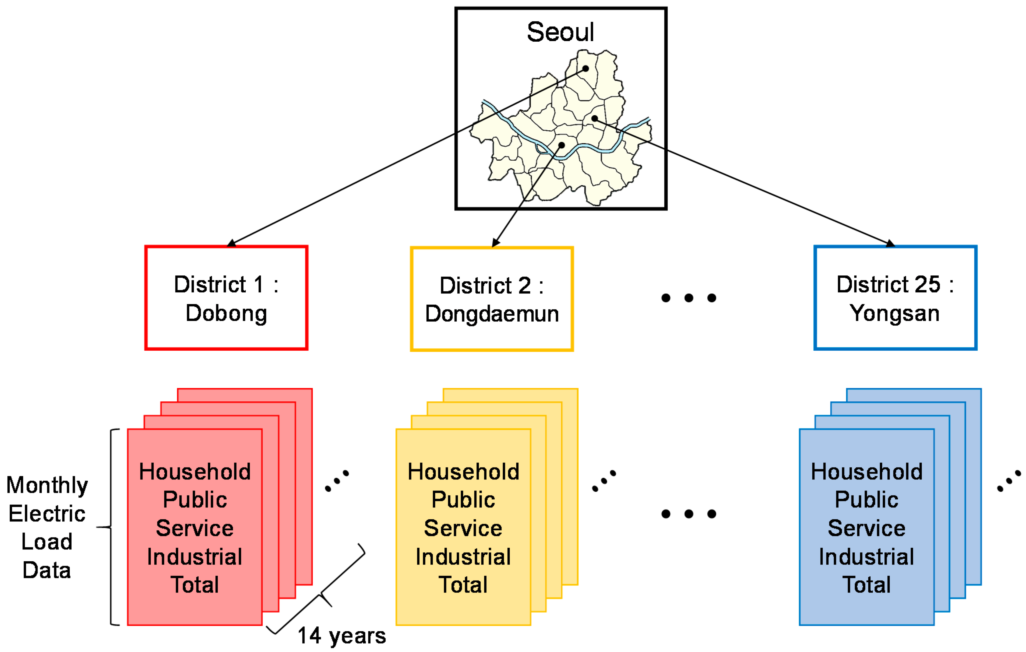
In this section, we first describe the dataset we used to construct our monthly load forecasting model. The dataset, which is provided by Seoul, contains the monthly electric load of 25 districts in Seoul from January 2005 to December 2018. The dataset can be divided into five categories: household, public, industrial, service, and total [43]. Figure 1 illustrates the details of the dataset. The household dataset comprises the monthly electricity consumption of purely residential customers. The public dataset contains the monthly electricity consumption for public purposes, such as social infrastructures and government organizations. Likewise, the industrial dataset reveals the monthly electricity consumption for mining, manufacturing, construction, and so on. The service dataset includes the monthly electricity consumption for water/wastewater treatment, fast transit systems, commercial offices, and retail buildings. Finally, the total dataset represents the sum of electricity consumption in only these four categories. As a result, the dataset comprises 125 pieces of sequence data for 14 years covering five categories and 25 districts and is used as source domains for transfer learning.

3.1. Input Variable Configuration

3.1.1. Calendar Data

In general, the amount of electricity consumption is determined by diverse factors. Among them, we considered three major factors. The first major factor is calendar data, such as the year, month, season, number of days, number of weekends, and number of holidays. The data are summarized with a brief description of the data representation in

Table 2. Calendar data.

No.	Input Variable	Description
1	Year	Integer [5:18]
2	Month	Integer [1:12]
3	Monthx	Continuous on [−1:1]
4	Monthy	Continuous on [−1:1]
5	Spring	Binary
6	Summer	Binary
7	Fall	Binary
8	Winter	Binary
9	No. of Days	Integer
10	No. of Mondays	Integer
11	No. of Tuesdays	Integer
12	No. of Wednesdays	Integer
13	No. of Thursdays	Integer
14	No. of Fridays	Integer
15	No. of Saturdays	Integer
16	No. of Sundays	Integer
17	No. of holidays on Mondays	Integer
18	No. of holidays on Tuesdays	Integer
19	No. of holidays on Wednesdays	Integer
20	No. of holidays on Thursdays	Integer
21	No. of holidays on Fridays	Integer
22	No. of Holidays	Integer
23	No. of weekdays	Integer
24	Maximum holiday length	Integer

.

Months have periodic properties [44]. For example, because December and January are temporally adjacent to each other, they have similar characteristics in terms of temperature and season. However, if we represent them numerically using 12 and 1, the difference in the categorical format becomes 11. To reflect this periodicity, we transform the month data into continuous data using Equation (1) and Equation (2) [45]:

$${\mathrm{Month}}_x=\sin \left(\frac{360}{12}\times \mathrm{Month}\right)$$

(1)

$${\mathrm{Month}}_y=\cos \left(\frac{360}{12}\times \mathrm{Month}\right)$$

(2)

Additionally, electricity consumption is usually reduced on holidays. Hence, the number of days and holidays in a month is related to the electricity consumption of the month [46]. In particular, because the number of holidays on weekdays may significantly affect the model, we also considered the number of holidays on weekdays for input variables. In addition, the extended holiday season is likely to generate a different electricity demand pattern than usual. Thus, the maximum holiday length for the month was also considered. We collected the holiday data from the website Time and Date (https://www.timeanddate.com). Consequently, we chose 24 input variables from the calendar data.

3.1.2. Population Data

The second factor that we considered for the model construction was the population data for a district [47]. The population data for the districts in Seoul are available from the Seoul Open Data Plaza (http://data.seoul.go.kr/).

Table 3. Input variables of population data.

No.	Input Variable	Description
1	Population	Annual
2	District area	Annual
3	Population density	Annual
4	In-migration	Monthly
5	Out-migration	Monthly
6	Net migration	Monthly

presents the input variables representing the population data, which include the population, area of the district, population density, in-migration, out-migration, and net migration. These data are determined in March each year based on the ID card information. The two types of population data are annual and monthly. The annual population data contain the population, district area, and population density. Monthly population data contain in-migration, out-migration, and net migration. The population in a district is highly correlated with the electricity consumption of that district. Still, we considered the monthly population data for a more detailed analysis.

3.1.3. Weather Data

The last factor is the weather data, such as temperature, humidity, and precipitation [48]. We collected the monthly weather data from the Korea Meteorological Administration (KMA). The KMA provides diverse types of forecasts, such as three-day ahead, mid-term, and long-range forecasts, depending on the time resolution. The long-range forecast consists of the one-month and three-month outlooks. We used the one-month outlook forecast for MTLF to provide a monthly weather forecast. The one-month outlook included the average temperature, average maximum temperature, average minimum temperature, and total precipitation for one month. We used them as the weather data.

3.2. Model Construction

In this paper, we aim to construct a forecasting model for a specific category of district. Hence, the target domain is represented by the district name and electricity category, and other combinations of districts and categories become the source domain. As we mentioned, we have a total of 125 combinations from 25 districts and five categories. We first constructed a monthly electric load forecasting model using similar electric load data from the remaining 124 electric load data, which are the source domains. To do this, we first divided each source data and target data into a training and a test set. To find similar load data from the source domains, we calculated the PCCs between the training sets of the source data and the target data. Then, using the selected source data, we constructed a DNN-based forecasting model. Finally, we fine-tuned the forecasting model using the training set of the target data and evaluated the model using the test set of the target data. The overall steps for constructing our model are illustrated in Figure 2.

3.2.1. Deep Neural Network

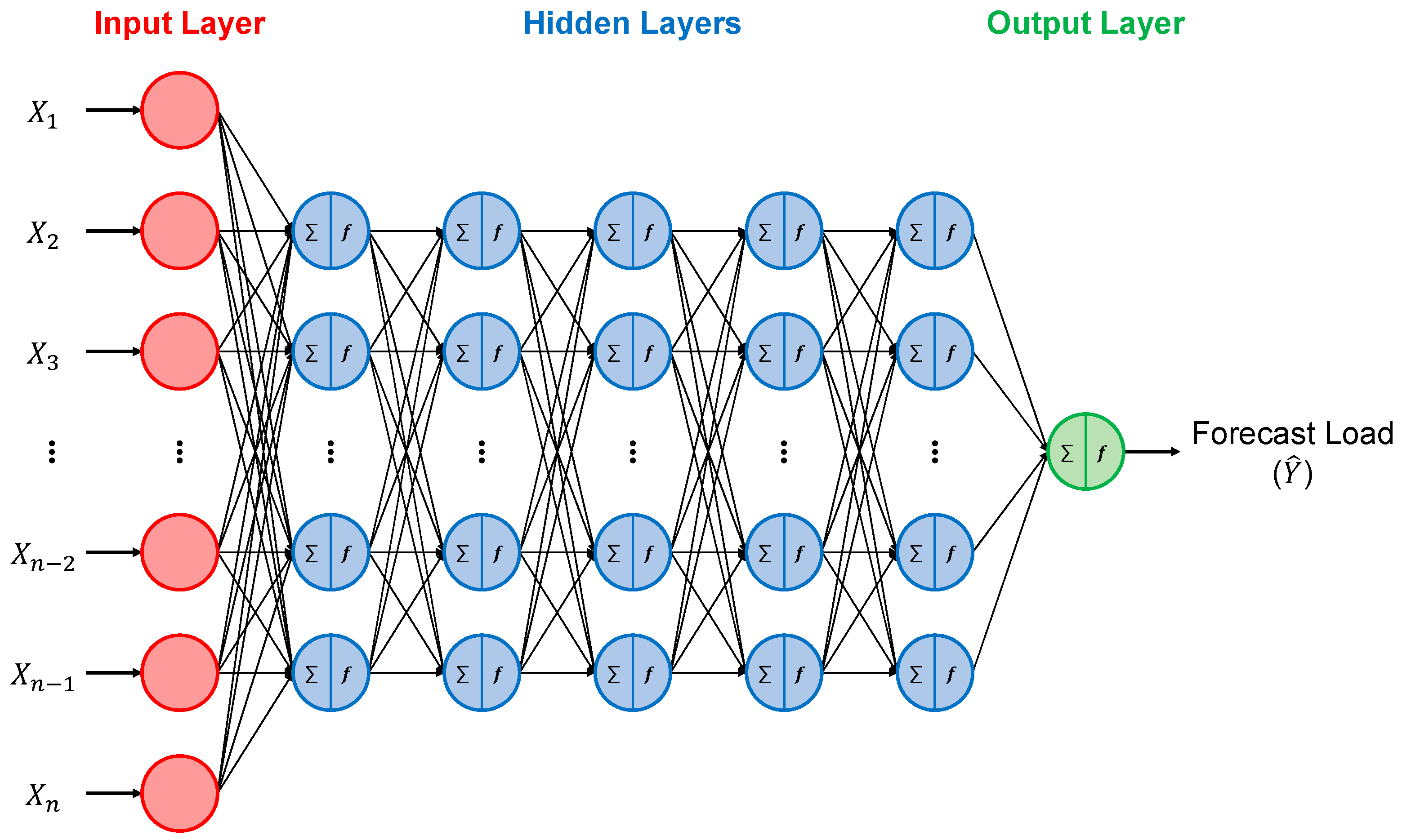
The artificial neural network is a machine-learning algorithm that imitates the human brain and consists of three layers: an input layer, one or more hidden layers, and an output layer [49,50]. Each layer consists of several nodes called perceptrons. Each node takes values from the nodes in the previous layer and determines an activation for the next nodes through a node activation function, such as a sigmoid function, hyperbolic tangent function, rectified linear unit (ReLU), exponential linear unit (ELU), scaled exponential linear unit (SELU), and so on. This process is repeated and the activation of the nodes in the final layer (the output layer) produces the desired outputs. If the number of hidden layers in the ANN is at least two, the network is called a DNN [50]. Figure 3 illustrates a typical DNN structure for MTLF. The more hidden layers in the DNN, the more complex the network becomes. Increasing the network complexity may improve the performance of the network. However, if the structure of DNN is more complex than necessary, the model could exhibit poor performance for unseen data, called overfitting [51]. Consequently, selecting the proper number of hidden layers is essential.

Various hyper-parameters must be considered to construct a DNN-based MTLF model, such as the number of hidden layers, number of nodes in the hidden layers, and activation function. To determine the hyper-parameters of the DNN model, we performed several comparative experiments. We set the number of hidden layers to 3, 4, 5, and 6, and considered SELU, ReLU, and ELU as activation functions.

Table 4. Performance comparison according to hyper-parameters.

Activation Function.	No. of Hidden Layers	MAPE	NRMSE
ELU	3	7.02	8.54
	4	6.93	8.48
	5	6.61	8.22
	6	6.80	8.35
ReLU	3	6.96	8.46
	4	6.96	8.46
	5	6.66	8.23
	6	6.83	8.43
SELU	3	7.05	8.67
	4	6.96	8.60
	5	6.52	8.11
	6	6.67	8.29

shows the results. The number of hidden layers is set to five, and the activation function in a multilayer perceptron is SELU [49]. Compared with the ReLU and ELU functions, which are typically used in DNNs, SELU is linear and increases the convergence speed of the stochastic gradient descent. The SELU is defined by Equation (3), where $\alpha$ and $\lambda$ are fixed constants, and $x$ is the input value. In the node configuration of the DNN model, the input layer comprises 33 nodes, and the hidden layer comprises 22 nodes per layer by applying two-thirds of the number of nodes of the input layer [52,53]. The output layer has only one node. Furthermore, we set the rest of the hyper-parameters as follows: batch size to 12, epoch to 1000, learning rate to 0.0001, and optimizer to adaptive moment estimation (Adam). We use the mean squared error (MSE) as a loss function, which is defined in Equation (4), where n is the number of observations and $y_i$ and ${\widehat{y}}_i$ are the actual and predicted values at time i:

$$f\left(\alpha ,x\right)=\lambda \{\begin{array}{c}x for x>0\\ \alpha e^x-\alpha for x\le 0\end{array},$$

(3)

$$\mathrm{MSE}=\frac{1}{n}{\sum }_{i=1}^n{(y_i-{\widehat{y}}_i)}^2 .$$

(4)

3.2.2. Transfer Learning

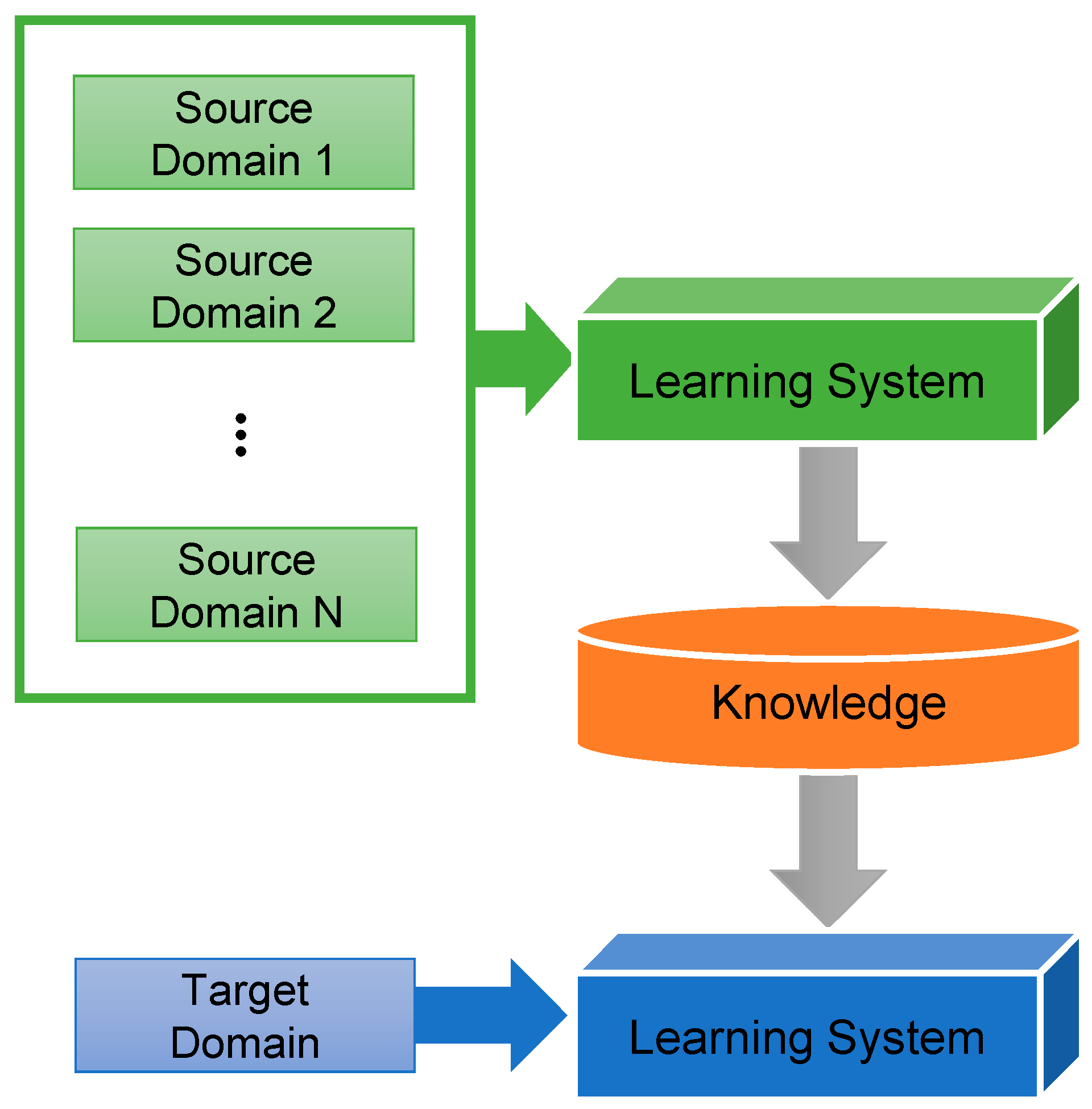
When limited data are available from the target domain for training, adaptation techniques, such as transfer learning, can be employed to improve the performance of a forecasting model [34,54]. Figure 4 illustrates a typical structure for transfer learning that uses the weights generated by neural networks trained using a large dataset similar to the target domain dataset. This process is called pre-training.

Then, the pre-trained network is trained again using the smaller target domain dataset. This process is called fine-tuning. When the data in the target domain and the source domain are similar, the resulting model could exhibit satisfactory performance. Thus, to find similar source domain data, correlation analysis methods, such as the PCC analysis, can be used to determine the similarity between two domains [34,55]. The PCC analysis is defined by Equation (5), where R_XY denotes the PCC between X and Y, n is the number of observations, and X_i and Y_i are the values at time i. Moreover, $\overline{X}$ and $\overline{Y}$ are the mean values of X and Y, respectively:

$$R_{XY}=\frac{{\sum }_i^n\left(X_i-\overline{X}\right)\left(Y_i-\overline{Y}\right)}{\sqrt{{\sum }_i^n{\left(X_i-\overline{X}\right)}^2}\sqrt{{\sum }_i^n{\left(Y_i-\overline{Y}\right)}^2}} .$$

(5)

The PCC is used to measure the linear correlation between two variables X and Y. It has a value between +1 and −1. Whereas a value of +1 (−1) indicates the total positive (negative) linear correlation between them, 0 indicates no linear correlation. Figure 5 illustrates an example of constructing a transfer learning-based DNN model, where $X_{i,S}$ and $X_{i,T}$ are the input of the source domain and the target domain at time i, respectively. $Y_{i,S}$ and $Y_{i,T}$ are the output of the source domain and the target domain at time i, respectively. When selecting the source domain, to consider all possible positive and negative trends, we selected domains with an absolute value of PCC close to 1. Using the selected source domains as a training set, we pre-trained the DNN model and fine-tuned the DNN model using a training set for the target domain.

4. Experimental Results

To evaluate the effectiveness of our model, we performed very extensive experiments. For the experiments, we collected five categories of monthly electric load data for 25 districts in Seoul from January 2005 to December 2018. Among them, we used the data from January 2005 to December 2016 as a training set and the data from January 2017 to December 2018 as a testing set. In the experiment, we considered every combination of district and category as a target domain and the other data as source domains. All experiments were performed in Python 3.7.6, and the models were constructed using TensorFlow 1.13.1.

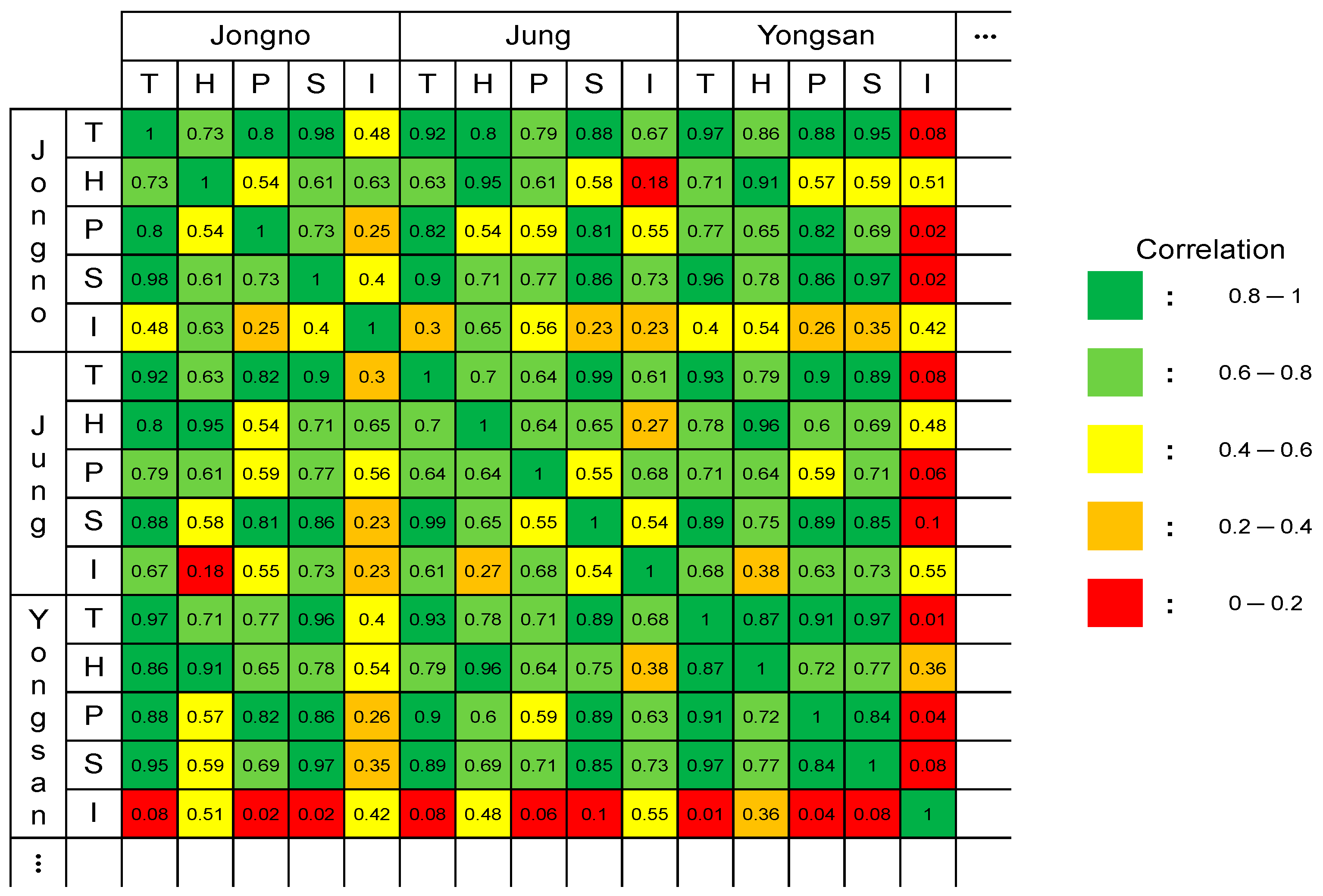
Figure 6 reveals part of a table containing PCC values calculated for the 125 domains. Each cell is marked with distinct colors according to the PCC value. The figure schematically shows the data characteristics by district and category. For instance, Jongno’s total is very similar to most categories of other districts because they have high PCC values. In contrast, Yongsan’s industrial is very different from most categories of other districts because they show low PCC values. This indicates that the Jongno’s total data are suitable for transfer learning, while the Yongsan’s industrial data are not. Meanwhile, Jongno’s industrial is not similar to Jung’s industrial, even though they belong to the same category. Rather, it is more similar to Jung’s service even though they belong to different categories. As a result, electric data from various domains can be effectively used for transfer learning if the similarity between data is well considered.

In addition, to observe the effect of the number of data for training the forecasting model, we constructed three different DNN models by selecting the top 10 (DNN_T10), 20 (DNN_T20), and 30 (DNN_T30) most similar domains in terms of PCC.

Table 5. Averages of the highest 10, 20, and 30 Pearson correlation coefficients for each district.

District	Top 10 PCCs	Top 20 PCCs	Top 30 PCCs
Jongno	0.89	0.86	0.84
Jung	0.93	0.91	0.89
Yongsan	0.92	0.87	0.83
Seongdong	0.72	0.69	0.67
Gwangjin	0.87	0.84	0.82
Dongdaemun	0.93	0.91	0.88
Jungnang	0.89	0.87	0.85
Seongbuk	0.91	0.89	0.87
Gangbuk	0.93	0.90	0.88
Dobong	0.82	0.77	0.73
Nowon	0.92	0.90	0.88
Eunpyeong	0.88	0.85	0.82
Seodaemun	0.89	0.85	0.82
Mapo	0.89	0.84	0.80
Yangcheon	0.90	0.87	0.85
Gangseo	0.85	0.79	0.73
Guro	0.91	0.85	0.80
Geumcheon	0.86	0.82	0.78
Yeongdeungpo	0.92	0.87	0.83
Dongjak	0.91	0.86	0.82
Gwanak	0.93	0.90	0.87
Seocho	0.81	0.79	0.77
Gangnam	0.91	0.88	0.85
Songpa	0.88	0.83	0.78
Gangdong	0.92	0.90	0.88

lists the average of the highest 10, 20, and 30 PCC values in the five categories for each district.

For the performance comparison, we considered the mean absolute percentage error (MAPE) and the normalized root mean squared error (NRMSE) [20,50]. The MAPE and NRMSE are defined by Equations (6) and (7), where n is the number of observations, $y_i$ and ${\widehat{y}}_i$ are the actual and predicted values at time i, respectively, and $\overline{y}$ is the mean of the actual values:

$$\mathrm{MAPE}=\frac{100}{n}{\displaystyle \sum }_{i=1}^n\left|\frac{y_i-{\widehat{y}}_i}{y_i}\right|$$

(6)

$$\mathrm{NRMSE}=\frac{100}{\overline{y}}\sqrt{\frac{{\sum }_i^n{\left(y_i-{\widehat{y}}_i\right)}^2}{n}} .$$

(7)

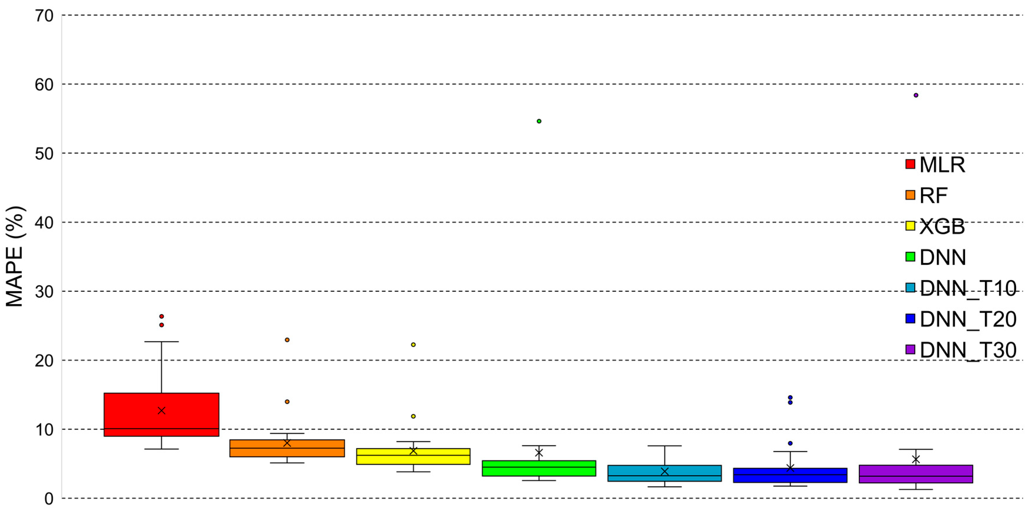
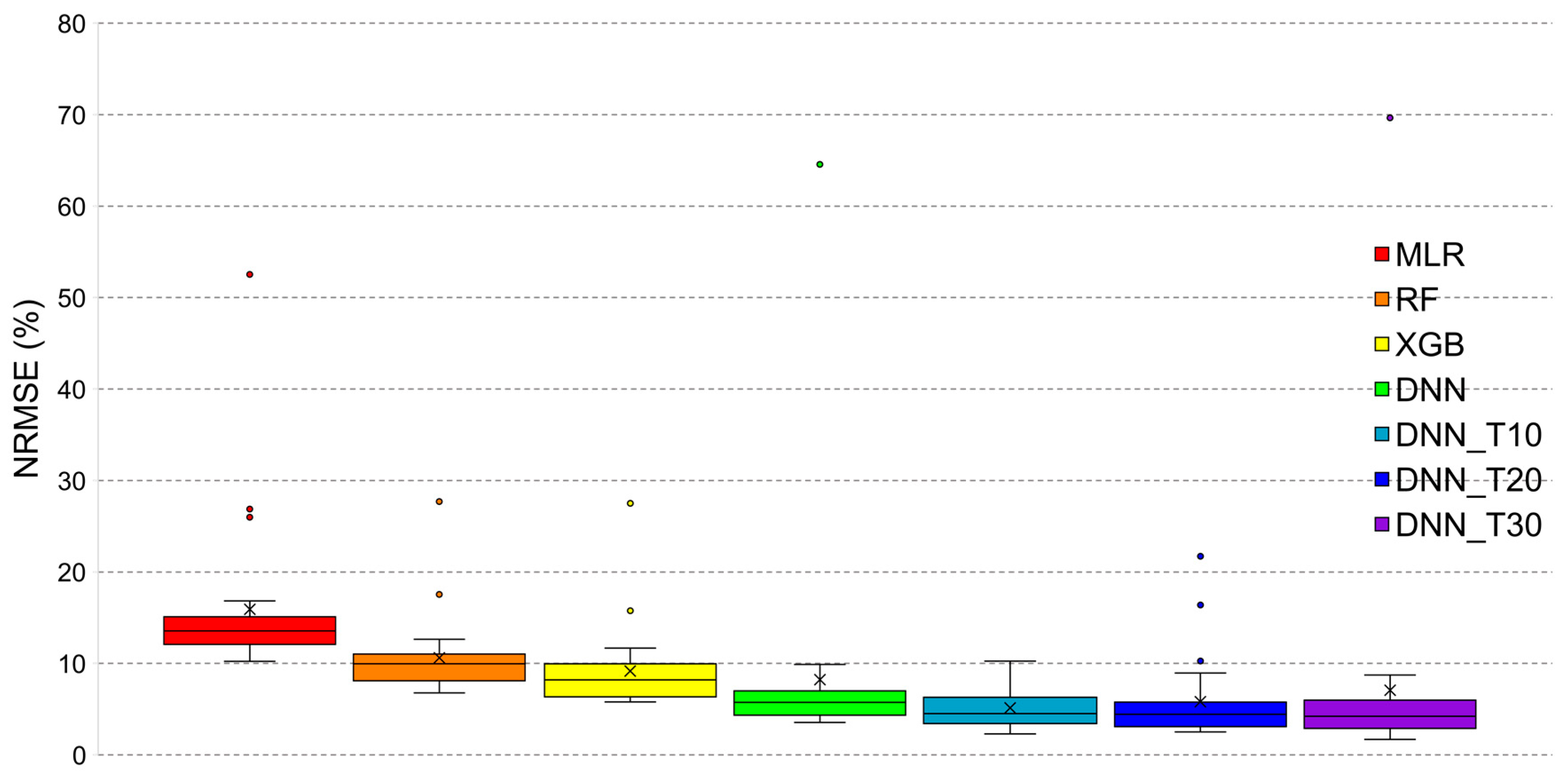
In addition to these three models, we considered four more forecasting models for comparison [56]: multiple linear regression (MLR), RF, extreme gradient boost (XGB), and baseline DNN. We calculated the MAPE and NRMSE values for all categories and then calculated the average value for each district.

Table 6. Average of mean absolute percentage errors (MAPE, unit: %) of five datasets in each district.

District	Forecasting Model
	MLR	RF	XGB	DNN	DNN_T10	DNN_T20	DNN_T30
Jongno	10.32	8.22	7.44	3.74	2.56	3.44	4.07
Jung	9.64	7.03	5.65	6.47	2.66	2.97	2.19
Yongsan	9.43	6.62	6.57	3.62	3.42	3.16	2.86
Seongdong	20.74	22.95	22.24	5.28	5.29	13.88	6.94
Gwangjin	9.10	6.05	4.49	5.20	2.01	1.84	2.38
Dongdaemun	8.22	6.47	5.31	2.56	2.36	1.76	1.90
Jungnang	8.38	5.87	4.15	3.22	3.59	3.52	1.56
Seongbuk	9.16	5.97	4.32	3.10	1.66	2.09	1.98
Gangbuk	9.05	9.39	8.21	3.08	2.28	2.57	1.46
Dobong	8.47	8.38	6.83	4.39	3.18	4.32	4.83
Nowon	8.20	5.45	4.03	4.30	3.20	1.86	1.26
Eunpyeong	10.21	8.89	7.55	5.22	3.74	4.05	4.71
Seodaemun	7.13	5.12	3.82	7.62	2.17	2.85	2.51
Mapo	10.19	8.71	7.05	3.77	4.12	3.90	3.81
Yangcheon	9.31	8.36	6.79	3.21	2.99	3.15	3.20
Gangseo	26.35	13.99	11.87	7.27	7.10	6.77	7.09
Guro	22.69	7.73	6.21	5.23	7.14	7.96	4.96
Geumcheon	10.10	8.01	6.98	4.50	4.10	4.33	3.72
Yeongdeungpo	10.09	5.37	4.00	4.87	4.23	2.02	2.95
Dongjak	25.26	5.51	6.13	6.96	6.21	6.50	5.70
Gwanak	8.90	8.55	6.03	3.11	2.83	2.36	2.26
Seocho	25.10	6.27	7.01	54.63	7.20	14.59	58.38
Gangnam	11.25	6.14	5.50	2.90	2.19	3.40	3.26
Songpa	19.18	7.80	7.33	5.60	7.60	4.03	4.15
Gangdong	11.02	7.25	6.11	4.85	3.25	2.22	2.83

DNN: deep neural network; DNN_T10: DNN pre-trained using top 10 similar data; DNN_T20: DNN pre-trained using top 20 similar data; DNN_T30: DNN pre-trained using top 30 similar data; MLR: multiple linear regression, RF: random forest, XGB: extreme gradient boosting.

and

Table 7. Average of normalized root mean squared errors (NRMSE, Unit: %) of five datasets in each district.

District	Forecasting Model
	MLR	RF	XGB	DNN	DNN_T10	DNN_T20	DNN_T30
Jongno	13.82	10.87	10.03	4.69	3.50	4.44	5.16
Jung	14.72	9.97	8.20	8.25	3.40	4.06	2.70
Yongsan	11.59	8.99	8.68	4.85	4.62	4.34	3.77
Seongdong	25.99	27.69	27.5	6.65	7.42	16.39	8.19
Gwangjin	12.24	8.01	6.38	6.58	2.71	2.71	3.46
Dongdaemun	12.09	9.51	7.85	3.55	3.43	2.50	2.48
Jungnang	11.90	7.75	6.01	4.37	4.62	4.71	2.09
Seongbuk	12.43	8.19	6.28	3.87	2.29	2.70	2.67
Gangbuk	13.56	12.64	11.68	4.33	2.94	3.44	1.99
Dobong	11.22	10.4	8.54	5.67	4.52	5.76	5.79
Nowon	11.69	7.55	5.88	5.75	3.84	2.60	1.69
Eunpyeong	13.16	12.18	10.76	6.70	5.07	5.33	6.15
Seodaemun	10.22	7.42	5.78	9.43	2.8	3.70	3.53
Mapo	15.07	12.18	9.91	4.88	5.18	5.68	5.34
Yangcheon	12.63	10.77	8.78	3.99	3.88	4.36	4.21
Gangseo	26.87	17.54	15.75	9.89	9.41	8.94	8.72
Guro	15.13	9.62	7.90	7.04	9.39	10.27	6.48
Geumcheon	14.28	10.67	9.38	5.72	5.11	5.77	4.53
Yeongdeungpo	12.80	7.84	5.80	5.98	5.06	2.68	3.72
Dongjak	16.82	8.29	6.31	8.05	8.02	7.13	7.41
Gwanak	12.09	11.18	8.13	4.12	3.72	3.28	3.07
Seocho	52.53	6.78	7.15	64.56	10.26	21.71	69.66
Gangnam	13.83	8.43	7.32	3.86	3.08	4.49	4.44
Songpa	16.19	10.73	10.2	6.95	9.98	5.71	5.56
Gangdong	14.8	10.06	8.65	5.80	4.34	2.90	3.61

DNN: deep neural network; DNN_T10: DNN pre-trained using top 10 similar data; DNN_T20: DNN pre-trained using top 20 similar data; DNN_T30: DNN pre-trained using top 30 similar data; MLR: multiple linear regression, RF: random forest, XGB: extreme gradient boosting.

present the average MAPEs and NRMSEs of five datasets for each district. The most commonly used method for tuning hyper-parameters is a grid search, which tries all possible combinations of the hyper-parameters of interest. Therefore, we selected the optimal hyper-parameters for the RF and XGB models using the grid search with cross-validation. The hyper-parameter tuning method, which divides data into training, validation, and test sets, can cause the problem of overfitting the validation set. To prevent this problem, we divided the data into training and test sets, and then used 5-fold cross-validation for the training data. Figure 7 and Figure 8 illustrate the box plots for the MAPE and NRMSE of the forecasting models. Our three transfer learning-based MTLF models exhibit better prediction performance than baseline DNN and other machine-learning-based models.

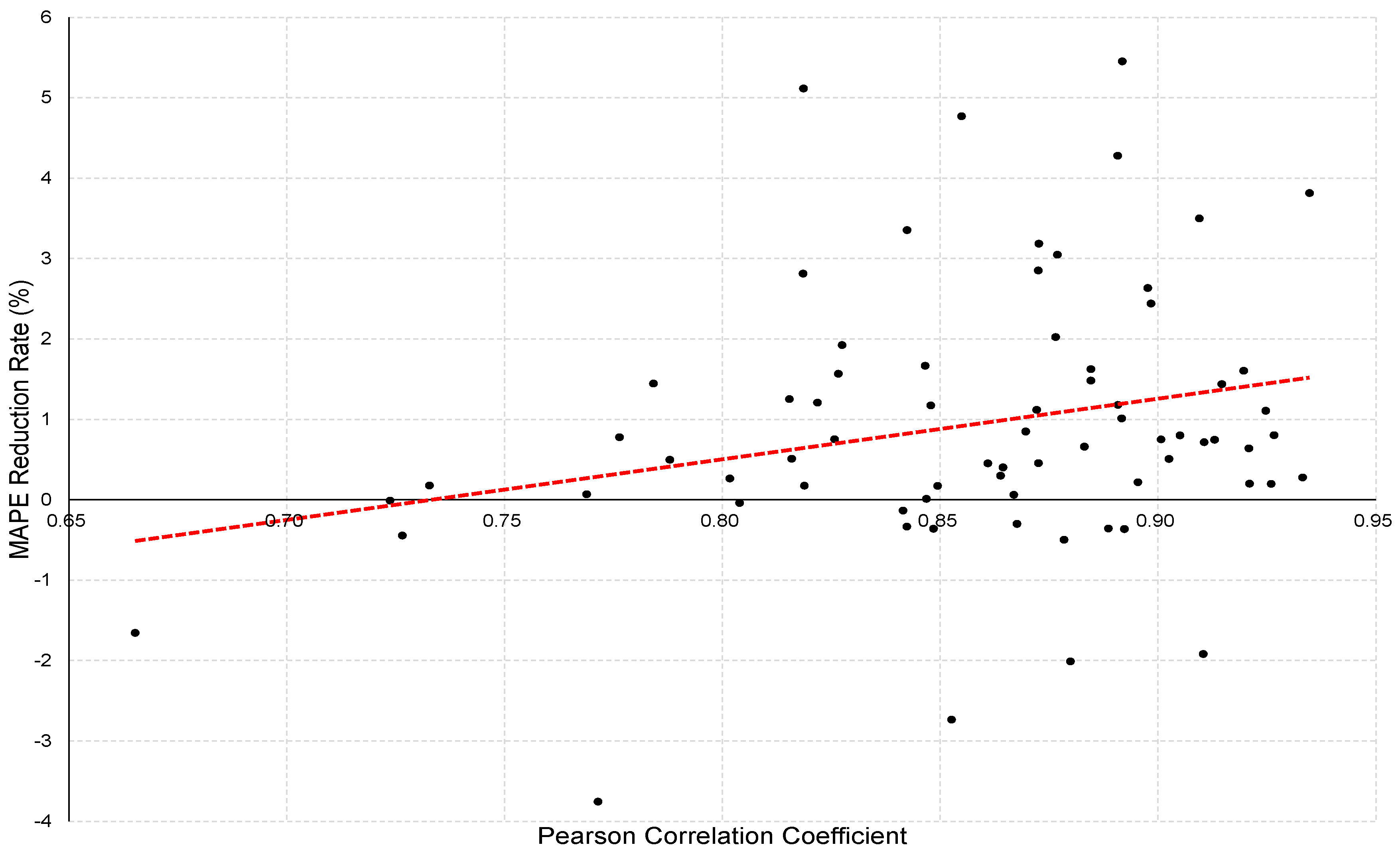
Figure 9 illustrates the trend intuitively by presenting the MAPE reduction rate for PCC values for DNN_T10, 20, and 30. The x-axis represents the PCC, and the y-axis represents the MAPE reduction rate, with each point representing the MAPE reduction rate for each PCC of the proposed models. The red line in the middle represents the trend line of the MAPE values. Figure 9 depicts a positive trend line slope, so the increase in the PCC value corresponding with transfer learning is closely related to the improvement in performance.

5. Conclusions

Because collecting sufficient monthly electricity consumption data is challenging due to the long recording period, it is difficult to build a sophisticated forecasting model based on an AI technique. To address this issue, in this study, we developed transfer-learning-based DNN models for monthly load forecasting. We used monthly electric load data collected for 14 years from Seoul public data. We configured the 33 input variables of three types, and constructed DNN-based MTLF models of 22 hidden nodes within five hidden layers. We considered the PCC to determine the similarity between the two domains. Then, we determined the top 10, 20, and 30 values with the highest PCC values as the source domains. We concatenated them to develop a training set for pre-training the DNN model. The pre-trained DNN model was fine-tuned using a training set for the target domain. We compared the performance of the proposed models with that of the machine-learning-based models, such as MLR, RF, and XGB, and a basic DNN model. We adopted the MAPE and NRMSE, which are the most popular performance metrics, to compare the prediction performance. We demonstrated that our model outperforms the existing machine-learning-based models and the base DNN model. Consequently, we conclude that the prediction performance improved when using transfer learning compared to the basic DNN.

In future studies, we plan to collect additional datasets from other regions and then to verify that our model is available to different datasets. Furthermore, by discussing other correlation coefficients, we can discover which correlation coefficients are useful for transfer learning.

References

- Desai, S.; Alhadad, R.; Mahmood, A.; Chilamkurti, N.; Rho, S. Multi-state energy classifier to evaluate the performance of the NILM algorithm. Sensors 2019, 19, 5236. [Google Scholar] [CrossRef] [PubMed] [Green Version]
- Udara Willhelm Abeydeera, L.H.; Wadu Mesthrige, J.; Samarasinghalage, T.I. Global research on carbon emissions: A scientometric review. Sustainability 2019, 11, 3972. [Google Scholar] [CrossRef] [Green Version]
- Rathore, M.M.; Ahmad, A.; Paul, A.; Rho, S. Urban planning and building smart cities based on the Internet of Things using Big Data analytics. Comput. Netw. 2016, 101, 63–80. [Google Scholar] [CrossRef]
- Talari, S.; Shafie-khah, M.; Siano, P.; Loia, V.; Tommasetti, A.; Catalão, J.P.S. A review of smart cities based on the internet of things concept. Energies 2017, 10, 421. [Google Scholar] [CrossRef] [Green Version]
- Bracco, S.; Delfino, F.; Laiolo, P.; Morini, A. Planning & Open-Air demonstrating smart city sustainable districts. Sustainability 2018, 10, 4636. [Google Scholar] [CrossRef] [Green Version]
- Cho, E.; Park, S.; Rew, J.; Park, C.; Lee, S.; Park, Y. Towards a sustainable open platform for location intelligence and convergence. In Proceedings of the 2018 International Conference on Information and Communication Technology Convergence (ICTC), Jeju, Korea, 17–19 October 2018; pp. 1411–1413. [Google Scholar] [CrossRef]
- Renaudin, V.; Marbel, R.; Ben-Moshe, B.; Zheng, X.; Ye, F.; Kuang, J.; Li, Y.; Niu, X.; Landa, V.; Hacohen, S.; et al. Evaluating indoor positioning systems in a shopping mall: The lessons learned from the IPIN 2018 competition. IEEE Access 2019, 7, 148594–148628. [Google Scholar] [CrossRef]
- Jun, S.; Rew, J.; Hwang, E. Runner’s Jukebox: A music player for running using pace recognition and music mixing. In Proceedings of the Seventh International Conferences on Advances in Multimedia (MMEDIA 2015), Barcelona, Spain, 19–24 April 2015; pp. 18–22. [Google Scholar]
- Kim, H.; Kim, W.; Rew, J.; Rho, S.; Hwang, E. Evaluation of hair and scalp condition based on microscopy image analysis. In Proceedings of the 2017 International Conference on Platform Technology and Service (PlatCon), Busan, Korea, 13–15 February 2017; pp. 1–4. [Google Scholar] [CrossRef]
- Kim, H.; Park, J.; Kim, H.; Hwang, E.; Rho, S. Robust facial landmark extraction scheme using multiple convolutional neural networks. Multimedia Tools Appl. 2018, 78, 3221–3238. [Google Scholar] [CrossRef]
- Kim, H.; Kim, H.; Hwang, E. Real-time shape tracking of facial landmarks. Multimed. Tools Appl. 2018. [Google Scholar] [CrossRef] [Green Version]
- Just, M.; Łuczak, A. Assessment of conditional dependence structures in commodity futures markets using copula-garch models and fuzzy clustering methods. Sustainability 2020, 12, 2571. [Google Scholar] [CrossRef] [Green Version]
- Khadam, U.; Iqbal, M.M.; Azam, M.A.; Khalad, S.; Rho, S.; Chilamkurti, N. Digital watermarking technique for text document protection using data mining analysis. IEEE Access 2019, 7, 64995. [Google Scholar] [CrossRef]
- Owusu, P.A.; Asumadu-Sarkodie, S. A review of renewable energy sources, sustainability issues and climate change mitigation. Cogent Eng. 2016, 3, 1167990. [Google Scholar] [CrossRef]
- Abam, F.I.; Nwankwojike, B.N.; Ohunakin, O.S.; Ojomu, S.A. Energy resource structure and on-going sustainable development policy in Nigeria: A review. Int. J. Energy Environ. Eng. 2014, 5, 102. [Google Scholar] [CrossRef] [Green Version]
- Ding, Z.; Lee, W.J.; Wang, J. Stochastic resource planning strategy to improve the efficiency of microgrid operation. IEEE Trans. Ind. Appl. 2015, 51, 1978–1986. [Google Scholar] [CrossRef]
- Promper, C.; Engel, D.; Green, R.C. Anomaly detection in smart grids with imbalanced data methods. In Proceedings of the 2017 IEEE Symposium Series on Computational Intelligence (SSCI), Honolulu, HI, USA, 27 November–1 December 2017. [Google Scholar] [CrossRef]
- Sorrell, S. Reducing energy demand: A review of issues, challenges and approaches. Renew. Sustain. Energy Rev. 2015, 47, 74–82. [Google Scholar] [CrossRef] [Green Version]
- Wang, Y.; Chen, Q.; Hong, T.; Kang, C. Review of smart meter data analytics: Applications, methodologies, and challenges. IEEE Trans. Smart Grid 2019, 10, 3125–3148. [Google Scholar] [CrossRef] [Green Version]
- Park, S.; Moon, J.; Jung, S.; Rho, S.; Baik, S.W.; Hwang, E. A two-stage industrial load forecasting scheme for day-ahead combined cooling, heating and power scheduling. Energies 2020, 13, 443. [Google Scholar] [CrossRef] [Green Version]
- Ahmad, A.S.; Hassan, M.Y.; Abdullah, M.P.; Rahman, H.A.; Hussin, F.; Abdullah, H.; Saidur, R. A review on applications of ANN and SVM for building electrical energy consumption forecasting. Renew. Sustain. Energy Rev. 2014, 33, 102–109. [Google Scholar] [CrossRef]
- Son, M.; Moon, J.; Jung, S.; Hwang, E. A short-term load forecasting scheme based on auto-encoder and random forest. In Proceedings of the 3rd International Conference on Applied Physics, System Science and Computers (APSAC), Dubrovnik, Croatia, 26–28 September 2018; pp. 138–144. [Google Scholar] [CrossRef]
- Ekonomou, L.; Christodoulou, C.A.; Mladenov, V. A short-term load forecasting method using artificial neural networks and wavelet analysis. Int. J. Power Syst. 2016, 1, 64–68. [Google Scholar]
- Borlea, I.; Buta, A.; Lustrea, B. Some aspects concerning mid term monthly load forecasting using ANN. In Proceedings of the International Conference on “Computer as a Tool”—EUROCON 2005, Belgrade, Serbia, 21–24 November 2005; pp. 253–256. [Google Scholar] [CrossRef]
- Lee, J.H.; Hancock, M.G.; Hu, M.C. Towards an effective framework for building smart cities: Lessons from Seoul and San Francisco. Technol. Forecast. Soc. 2014, 89, 80–99. [Google Scholar] [CrossRef]
- Kim, K.; Jung, J.-K.; Choi, J.Y. Impact of the smart city industry on the korean national economy: Input-output analysis. Sustainability 2016, 8, 649. [Google Scholar] [CrossRef] [Green Version]
- Khuntia, S.R.; Rueda, J.L.; van der Meijden, M.A.M.M. Forecasting the load of electrical power systems in mid- and long-term horizons: A review. IET Gener. Transm. Distrib. 2016, 10, 3971–3977. [Google Scholar] [CrossRef] [Green Version]
- Moon, J.; Kim, K.-H.; Kim, Y.; Hwang, E. A short-term electric load forecasting scheme using 2-stage predictive analytics. In Proceedings of the IEEE International Conference on Big Data and Smart Computing (BigComp), Shanghai, China, 15–17 January 2018; pp. 219–226. [Google Scholar] [CrossRef]
- Kim, J.; Moon, J.; Hwang, E.; Kang, P. Recurrent inception convolution neural network for multi short-term load forecasting. Energy Build. 2019, 194, 328–341. [Google Scholar] [CrossRef]
- Hossen, T.; Plathottam, S.J.; Angamuthu, R.K.; Ranganathan, P.; Salehfar, H. Short-term load forecasting using deep neural networks (DNN). In Proceedings of the 2017 North American Power Symposium, Morgantown, WV, USA, 17–19 September 2017; pp. 1–6. [Google Scholar] [CrossRef]
- Kuo, P.H.; Huang, C.J. A high precision artificial neural networks model for short-term energy load forecasting. Energies 2018, 11, 213. [Google Scholar] [CrossRef] [Green Version]
- Chitsaz, H.; Shaker, H.; Zareipour, H.; Wood, D.; Amjady, N. Short-term electricity load forecasting of buildings in microgrids. Energy Build 2015, 99, 50–60. [Google Scholar] [CrossRef]
- Hosein, S.; Hosein, P. Load forecasting using deep neural networks. In Proceedings of the IEEE Power & Energy Society Innovative Smart Grid Technologies Conference (ISGT), Washington, DC, USA, 23–26 April 2017; pp. 1–5. [Google Scholar] [CrossRef]
- Moon, J.; Kim, J.; Kang, P.; Hwang, E. Solving the cold-start problem in short-term load forecasting using tree-based methods. Energies 2020, 13, 886. [Google Scholar] [CrossRef] [Green Version]
- Pan, S.J.; Yang, Q. A survey on transfer learning. IEEE Trans. Knowl. Data Eng. 2010, 22, 1345–1359. [Google Scholar] [CrossRef]
- Damrongkulkamjorn, P.; Churueang, P. Monthly energy forecasting using decomposition method with application of seasonal ARIMA. In Proceedings of the 2005 International Power Engineering Conference, Singapore, 29 November–2 December 2005; pp. 224–229. [Google Scholar] [CrossRef]
- Dong, B.; Cao, C.; Lee, S.E. Applying support vector machines to predict building energy consumption in tropical region. Energy Build. 2005, 37, 545–553. [Google Scholar] [CrossRef]
- Ma, Y.; Yu, J.Q.; Yang, C.Y.; Wang, L. Study on power energy consumption model for large-scale public building. In Proceedings of the 2010 2nd International Workshop on Intelligent Systems and Applications, Wuhan, China, 22–23 May 2010; pp. 1–4. [Google Scholar] [CrossRef]
- Berriel, R.F.; Lopes, A.T.; Rodrigues, A.; Varejão, F.M.; Oliveira-Santos, T. Monthly energy consumption forecast: A deep learning approach. In Proceedings of the 2017 International Joint Conference on Neural Networks (IJCNN), Anchorage, AK, USA, 14–19 May 2017; pp. 4283–4290. [Google Scholar] [CrossRef]
- Mocanu, E.; Nguyen, P.H.; Kling, W.L.; Gibescu, M. Unsupervised energy prediction in a Smart Grid context using reinforcement cross-building transfer learning. Energy Build. 2016, 116, 646–655. [Google Scholar] [CrossRef] [Green Version]
- Ribeiro, M.; Grolinger, K.; ElYamany, H.F.; Higashino, W.A.; Capretz, M.A. Transfer learning with seasonal and trend adjustment for cross-building energy forecasting. Energy Build. 2018, 165, 352–363. [Google Scholar] [CrossRef]
- Hooshmand, A.; Sharma, R. Energy predictive models with limited data using transfer learning. In Proceedings of the Tenth ACM International Conference on Future Energy Systems (e-Energy ’19), Phoenix, AZ, USA, 25–28 June 2019; pp. 12–16. [Google Scholar] [CrossRef] [Green Version]
- Let’s Open, Collect and Share Seoul Public Data: Seoul Open Data Plaza. Available online: https://www.seoulsolution.kr/en/content/let%E2%80%99s-open-collect-and-share-seoul-public-data-seoul-open-data-plaza (accessed on 25 February 2020).
- Moon, J.; Park, J.; Hwang, E.; Jun, S. Forecasting power consumption for higher educational institutions based on machine learning. J. Supercomput. 2018, 74, 3778–3800. [Google Scholar] [CrossRef]
- Jung, S.; Moon, J.; Park, S.; Rho, S.; Baik, S.W.; Hwang, E. Bagging ensemble of multilayer perceptrons for missing electricity consumption data imputation. Sensors 2020, 20, 1772. [Google Scholar] [CrossRef] [PubMed] [Green Version]
- Dang-Ha, T.-H.; Bianchi, F.M.; Olsson, R. Local short term electricity load forecasting: Automatic approaches. In Proceedings of the 2017 International Joint Conference on Neural Networks (IJCNN), Anchorage, AK, USA, 14–19 May 2017; pp. 4267–4274. [Google Scholar] [CrossRef] [Green Version]
- Kermanshahi, B.; Iwamiya, H. Up to year 2020 load forecasting using neural nets. Int. J. Electr. Power Energy Syst. 2002, 24, 789–797. [Google Scholar] [CrossRef]
- Wang, P.; Liu, B.; Hong, T. Electric load forecasting with recency effect: A big data approach. Int. J. Forecast. 2016, 32, 585–597. [Google Scholar] [CrossRef] [Green Version]
- Moon, J.; Park, S.; Rho, S.; Hwang, E. A comparative analysis of artificial neural network architectures for building energy consumption forecasting. Int. J. Distrib. Sens. Netw. 2019, 15. [Google Scholar] [CrossRef] [Green Version]
- Moon, J.; Kim, Y.; Son, M.; Hwang, E. Hybrid short-term load forecasting scheme using random forest and multilayer perceptron. Energies 2018, 11, 3283. [Google Scholar] [CrossRef] [Green Version]
- Yasir, M.; Durrani, M.Y.; Afzal, S.; Maqsood, M.; Aadil, F.; Mehmood, I.; Rho, S. An intelligent event-sentiment-based daily foreign exchange rate forecasting system. Appl. Sci. 2019, 9, 2980. [Google Scholar] [CrossRef] [Green Version]
- Moon, J.; Jung, S.; Rew, J.; Rho, S.; Hwang, E. Combination of short-term load forecasting models based on a stacking ensemble approach. Energy Build. 2020, 216, 109921. [Google Scholar] [CrossRef]
- Heaton, J. Introduction to Neural Networks with Java; Heaton Research, Inc.: Chesterfield, MO, USA, 2008. [Google Scholar]
- Zhang, Y.; Luo, G. Short term power load prediction with knowledge transfer. Inf. Syst. 2015, 53, 161–169. [Google Scholar] [CrossRef]
- Zhi, X.; Yuexin, S.; Jin, M.; Lujie, Z.; Zijian, D. Research on the Pearson correlation coefficient evaluation method of analog signal in the process of unit peak load regulation. In Proceedings of the 2017 13th IEEE International Conference on Electronic Measurement & Instruments (ICEMI), Yangzhou, China, 20–22 October 2017; pp. 522–527. [Google Scholar] [CrossRef]
- Park, S.; Moon, J.; Hwang, E. 2-Stage electric load forecasting scheme for day-ahead cchp scheduling. In Proceedings of the 13th IEEE International Conference on Power Electronics and Drive Systems (PEDS), Toulouse, France, 9–12 July 2019. [Google Scholar] [CrossRef]
Figure 1.
Hierarchical structure of Seoul’s monthly electric load.
Figure 2.
Overall steps for monthly electric load forecasting.
Figure 3.
Typical deep neural network structure for monthly electric load forecasting.
Figure 4.
Process of transfer learning.
Figure 5.
Example of constructing a transfer learning-based deep neural network model.
Figure 6.
Example of the calculated Pearson correlation coefficient (PCC); T, H, P, S, and I represent the total, household, public, service, and industrial, respectively.
Figure 7.
Box plot of the mean absolute percentage error (MAPE) of the forecasting models; DNN: deep neural network; DNN_T10: DNN pre-trained using top 10 similar data; DNN_T20: DNN pre-trained using top 20 similar data; DNN_T30: DNN pre-trained using top 30 similar data; MLR: multiple linear regression, RF: random forest, XGB: extreme gradient boosting.
Figure 8.
Box plot of the normalized root mean squared error (NRMSE) of the forecasting models; DNN: deep neural network; DNN_T10: DNN pre-trained using top 10 similar data; DNN_T20: DNN pre-trained using top 20 similar data; DNN_T30: DNN pre-trained using top 30 similar data; MLR: multiple linear regression, RF: random forest, XGB: extreme gradient boosting.
Figure 9.
Mean Absolute percentage error (MAPE) reduction rate versus the Pearson correlation coefficient.