Spatiotemporal Dynamics of Precipitation in Southwest Arid-Agriculture Zones of Pakistan

Abstract

Investigation of spatiotemporal precipitation trends from a climate change perspective is essential, especially in those regions with rainfed agriculture in order to propose sustainable adaptation schemes. Some restrictive assumptions may hinder the efficacy of trend detection methods, so it could be supported with variability analysis to have a clear picture of the spatiotemporal precipitation dynamics rather than focusing on a single approach. Hence, in the current study, a spatiotemporal dynamic analysis of precipitation was carried out using trend detection methods (the innovative trend analysis method and Mann–Kendall test) and statistical indices (the consecutive disparity index, entropy-based variability index and absolute inter-variability index) in the southwest arid region of Pakistan. The results indicated that based on the monthly, annual and seasonal time series, no systematic precipitation pattern was observed across the whole study region. However, on average, an increasing trend was observed in the east plateau while decreasing in the west plateau. The variability analysis also signposted the higher variability in the case of the western plateau and coastal area compared to the east plateau. Based on the seasonal analysis, it was concluded that, on average, precipitation in the winter and spring season goes on decreasing with higher variability while a mixture of increasing and decreasing trends resulted for summer and autumn. Conclusively the study found that precipitation in the study area is more erratic and its behaviour abruptly changed over a short distance. Moreover, discrepancies and inconstancies were found in the selected trend detection approaches and variability indices. The results also indicated that climate change is going to seriously affect the region as a decreasing trend prevails in most of the cases and stations.

1. Introduction

An understanding of the characteristics of precipitation at the regional scale is essential for evaluating the interaction between different components of the hydrological cycle [1], as well as for the assessment of water demand, sustainable agriculture, water resources management and mitigation of floods and drought [2]. The monitoring of rainfall patterns at a continuous level is also vital to get a comprehensive understanding of climate variability; however, the investigation of regional precipitation variability is complex because it could be more erratic with significant spatiotemporal variation in the same region [3,4]. Generally, trend analysis methods and variability indexing approaches are used for the spatiotemporal analysis of precipitation dynamics at a regional and global scale [5,6].

Two types of trend analysis techniques, namely non-parametric and parametric approaches, are commonly used to define the characteristics of parameters to be analysed. Highly accurate, continuous, normally distributed and independent data are generally required for the parametric tests, which is often available in developing countries like Pakistan. On the other hand, non-parametric trend analysis has gained much popularity and attention in different climate change-related studies, just because of their accuracy, flexibility and repeatability [7,8,9]. Linear regression [10], Spearman’s rho test [11], cumulative sum based trend analysis approach [12], Mann–Kendall trend analysis approach [13] and, recently, an innovative trend analysis approach [14], are few of the non-parametric methods reported in the literature. For example, significant numbers of studies have been carried out to detect monthly, annual, and seasonal precipitation trends using the non-parametric Mann–Kendall test with the combination of Spearman’s Rho tests [15,16,17,18]. However, this method has some restrictive assumptions, e.g., time series length, seasonal cycle, serial indecencies and normality of time series distribution, but is still an effective and universally used trend detection method. In contrast, an innovative trend analysis approach [19] is simple and have the advantage of detecting a sub-series trend by graphical representations, but remaining outlier sensitive. An innovative trend analysis approach has been effectively applied to various water resources applications [14,19,20,21].

Generally, the trend analysis methods ignore the consecutive order of the numerical values; however, the chronological order provides a better illustration of the temporal behaviour of variables to be considered. For example, any precipitation series with a chronological order, and the same series with sorted values in descending or ascending order would have the same coefficient of variation, but climatic meanings could differ. The presence of extreme events, outliers and restrictive assumptions can also influence the efficiency of these methods. Moreover, using different approaches enable to have a clear indication of the spatiotemporal precipitation dynamics rather than focusing on a single approach. Hence, solely focusing on the ordered trend analysis methods may mislead and, therefore, should be supported with variability analysis to understand the temporal irregularity better. The variability analysis is statistically expressed both in relative and absolute terms [22] to examine the temporal anomalies of precipitation by keeping in view the consecutive order of the precipitation time series. The absolute statistical indices (e.g., standard deviation, absolute inter-annual variability and mean absolute deviation) could provide the degree to which precipitation amounts change across a region or over a timescale. Conclusively, variability indices in combination with trend analysis methods should be used to have a better understanding of precipitation in a specific region.

Like other parts of the worlds, a significant number of studies (

Table 1. Review of the literature regarding precipitation variability analysis in Pakistan (MK: Mann–Kendall; LR: Linear Regression).

Sr #	By	Region	Approach	Finding
1	[24]	Punjab, Pakistan	MK	No considerable trend was identified
2	[25]	Himalaya Region	MK	An increasing trend in annual precipitation
3	[26]	Himalaya and Hindu Kush-Karakoram	MK	The overall decrease in trend except for 1 basin
4	[27]	Himalaya region	MK with moving window, LR	Precipitation substantial increase at 1 out of 4 station
5	[28]	Hindu Kush-Karakoram region	LR and MK	Rise in annual precipitation during 1901–2010
6	[29]	Himalaya and Hindu Kush-Karakoram	MK	Increasing precipitation trend in annual and monsoon season
7	[30]	Himalaya and Hindu Kush-Karakoram	MK and LR	The decreasing trend in the wet day and inclination in precipitation intensity
8	[31]	Swat River	MK and Spearman’s rho test	A mix of increasing and decreasing trends
9	[32]	Himalaya and Hindu Kush-Karakoram	MK	Positive variation in rainfall extreme resulted in some regions
10	[33]	Himalaya and Hindu Kush-Karakoram	MK	A mixture of the trend at 5 selected station
11	[34]	Himalaya and Hindu Kush-Karakoram	LR	Increase in intensity, while a decrease in the frequency of heavy rainfall
12	[35]	Himalaya and Hindu Kush-Karakoram	LR	Increasing precipitation trend at 1 station while decreasing at two stations
13	[36]	Three stations of Balochistan	MK	Decreasing trend direction on an annual and seasonal basis
14	[37]	30 stations from all over Pakistan with three from west	ANOVA Dennett T3	A decrease in precipitation trends at the rate of 1.18 mm/year at three stations during 1961–1999
15	[38]	Himalaya and Hindu Kush-Karakoram	MK	The decrease in winter and annual precipitation and an increase in monsoon precipitation
16	[39]	Indus Basin of Pakistan	MK test	No significant trend was observed. However, increase in mean precipitation
17	[40]	Sub-Himalayan region of Pakistan	Modified MK test	Increase in extreme precipitation and dry days
18	[41]	Upper Indus Basin of Pakistan	MK test and ITA	A mixture of increasing and decreasing trend in precipitation extreme

) have been carried out to analyse the precipitation pattern in Pakistan and concluded that the precipitation regime all over Pakistan is more erratic and mainly controlled by the monsoon season [23]. The salient feature and findings of the studies performed in Pakistan are provided in Table 1. The scientific literature review showed that most of the studies were carried out using the Mann–Kendall test with a few studies using simple linear regression. Based on the literature discussions, a mixture of increasing as well as decreasing trends were observed, which indicates the need for further investigation. In addition to that, up to best of the authors’ knowledge, none of the studies used absolute statistical indices, e.g., the percentage of annual variability, relative variability index and precipitation concertation index, to explore a chronological sequence of values and to assess the average rate of change among consecutive values over the different regions of Pakistan. A large number of studies have been conducted in the northern area, especially Himalaya and Hindu Kush-Karakoram, while the southwest region of Pakistan is still deprived of any comprehensive research. The southwest region of Pakistan is generally categorised as the drought-prone arid agricultural region of the country and most vulnerable to hydrological hazards. It is also expected that due to climate change, water scarcity and drought situations could increase in this region in the 21st century. The precipitation of the southwest region is sparser, erratic and widely varies over a small distance. More than 85% of the population of this region lives in rural areas, who mainly depend on agriculture as their source of income and rangelands as a source of livestock feed. So, any climatic variation in the region can adversely disturb the population and livestock. Therefore, for mitigation and adaption planning, urgent attention is needed to assess the current and future dynamics of the meteorological variable in the region. Thus, the present study covers the southwest part of the country for analysing the precipitation dynamic at a monthly, annual and seasonal scale using an innovative trend approach, the Mann–Kendall method and variability indices.

2. Materials and Methods

2.1. Study Area

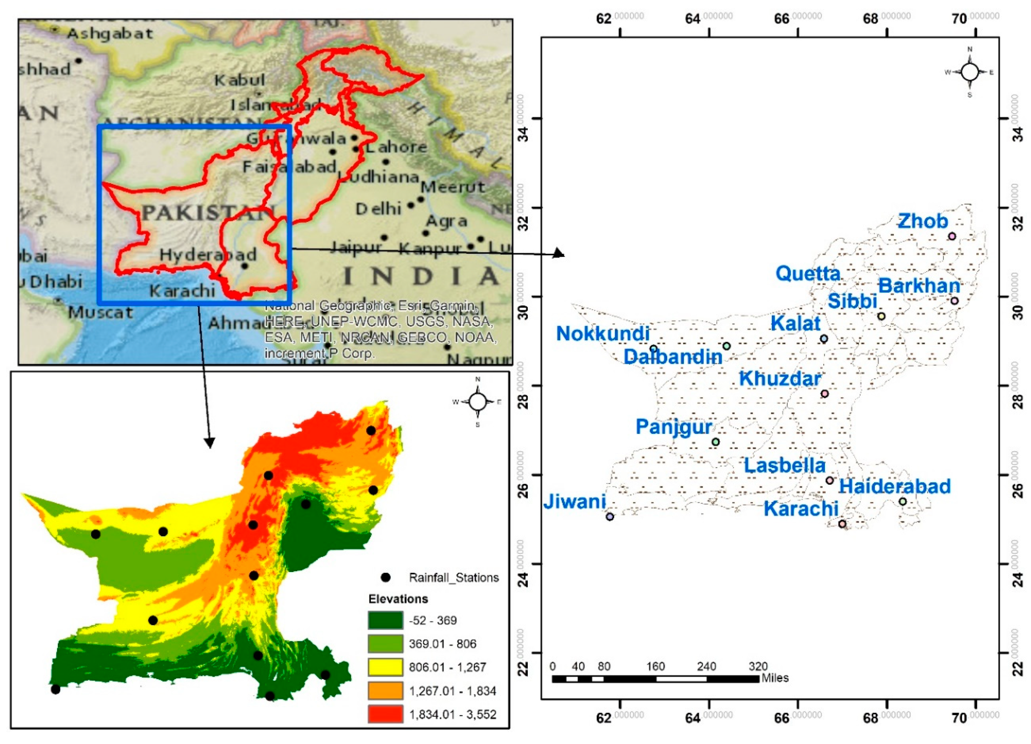
The southwest region of Pakistan mainly consists of the largest provinces (by area) of Pakistan, i.e., Balochistan and the southern part of Sindh (Figure 1, upper left). It is covering an area of 247,190 km², which is contributing 43.6% of the total landmass in Pakistan. It has a peculiar geomorpho-climatic location, including deserts, dry land, mountainous ranges, inland water bodies, woodland forests, forest, grassland and coastal plains. The mean sea level varies from −52 to 3552 m (Figure 1, lower left). The climate of the analysed region is continental, i.e., hot summers and cold winters in the upper highland area, while subtropical (warm summers and mild winters) in lowland and flat regions. The southwest region generally covers arid to hyper-arid areas with variable and scanty rainfall and experience erratic behaviours of extreme events. The average annual precipitation ranges from 100 mm (in low land and plain region) to 400 mm (in the highland region) with a maximum recorded temperature of 52 °C. Climate change has a significant social implication in most of the Southwest, mainly coastal areas, and it could cause an extreme hazard development if it remains unmanaged. Initially, the selected region is divided into the east plateau, west plateau and coastal area based on geographical locations. The Pakistan meteorological department has started monitoring climate change and variables associated with climate change indicators by installing a gauge station in a different part of the Southwest region; however, they are characterised by an insufficient and low gauge density due to complex terrain and social issues. So, for the better illustration of precipitation variability in the different climatic zone, we selected a total of thirteen (13) rain gauge stations (Figure 1, right, and

Table 2. Salient features of the selected stations in a southwest arid region of Pakistan.

Stations	Long	Lat	Elevation (m)	Record Period	Record Length (Years)
Barkhan	69.52	29.90	1097	1990–2018	29
Dalbandin	64.40	28.89	848	1981–2018	38
Jiwani	61.77	25.05	56	1981–2018	38
Kalat	66.59	29.05	2015	1981–2018	38
Khuzdar	66.61	27.82	1231	1981–2018	38
Lasbella	66.71	25.87	87	1981–2018	38
Nokkundi	62.75	28.83	682	1981–2018	38
Panjgur	64.15	26.73	968	1981–2018	38
Quetta	66.96	30.25	1626	1981–2018	38
Sibbi	67.88	29.55	133	1981–2018	38
Zhob	69.47	31.35	1405	1981–2018	38
Haiderabad	68.42	25.38	30	1981–2018	38
Karachi	66.93	24.90	11	1981–2018	38

). During the selection of stations, the quality and continuity (no missing information) of rainfall data was insured to avoid any misleading results.

2.2. Trend Analysis Approaches

To understand the current water resource developments in a region, it is necessary to find out the existence of a trend in meteorological variables. The non-parametric Mann–Kendall test [42,43] and the innovative trend analysis method were used to detect possible changes and trends in the precipitation series. The details of these approaches are given below.

2.2.1. Mann–Kendall Test

The Mann–Kendall test is commonly used for identifying trends in precipitation data series, because of its insensitivity to outliers, high degree of quantification and wide range [44]. The MK test tests whether to reject the null hypothesis (H₀), i.e., “no trend”, or accept the alternative hypothesis (H_a), i.e., “the trend exists”. The MK test statistic S is as mentioned in Equation (1). A positive value of S shows an increasing trend, while the negative value of S signposts a decreasing trend.

$$S={\displaystyle \sum _{k=1}^{n-1}{\displaystyle \sum _{k+1}^n\mathrm{sgn}}}\left(x_j-x_k\right)$$

(1)

$$sgn(x_j-x_k)=\{\begin{array}{ll}-1& if:(x_j-x_k)<0\\ 0& if:(x_j-x_k)=0\\ 1& if:(x_j-x_k)>0\end{array}$$

(2)

whereas n signifies the total numbers of observations in the time series, $x_j$ and $x_k$ are sequential values at time j and k; $sgn$ represent the sign function.

The standardised test statistic $Z$ (Equation (3)) is used to evaluate the significance of the trend in the data series.

$$Z=\{\begin{array}{ll}\frac{S-1}{\sqrt{{\sigma }_S^2}}& if:S<0\\ 0& if:S=0\\ \frac{S+1}{\sqrt{{\sigma }_S^2}}& if:S>0\end{array}$$

(3)

where ${\sigma }_S^2$ represents the variance of S (Equation (5)) and the mean value of S is represented by $E\left(S\right)$:

$$E\left(S\right)=0$$

(4)

$${\sigma }_S^2=n\left(n-1\right)\left(2n+5\right)-{\displaystyle \sum _{k=1}^p{t}_k\left(t_k-1\right)\left(2t_k-1\right)/18}$$

(5)

whereas p represents the tied group, t_k represents the total number of observation kth group.

The calculated standardized test statistic ($Z$) follows a normal distribution (mean = 0 and variance = 1). The positive and negative value of Z indicates the trend direction in the time series. This test statistic is used to test the null hypothesis using the significant level α (here at 5%) and the p-value. If the p-value < the significant level α, and $\left|Z\right|\le Z_{\alpha /2}$, then reject the null hypothesis.

In the current study, the MK test was applied by following the given steps to avoid any misleading results:

(1)

Initially, the homogeneity test, i.e., Standard Normal Homogeneity Test (SNHT) and Buishand test was applied to test for homogeneity in the precipitation series [31].

(2)

Then, Lag 1 autocorrelation was computed to check whether the selected precipitation series are serial independent or not at the 5% significance level.

(3)

If applicable, the data with a serial correlation was detrended, and a new blended series was obtained using a trend-free pre-whitening test (TFPW) as proposed by [16].

(4)

Lastly, the standardised test statistic $Z$ (Equation (3)) was then applied to check the significance of the trend at the 5% significance level.

2.2.2. Innovative Trend Analysis

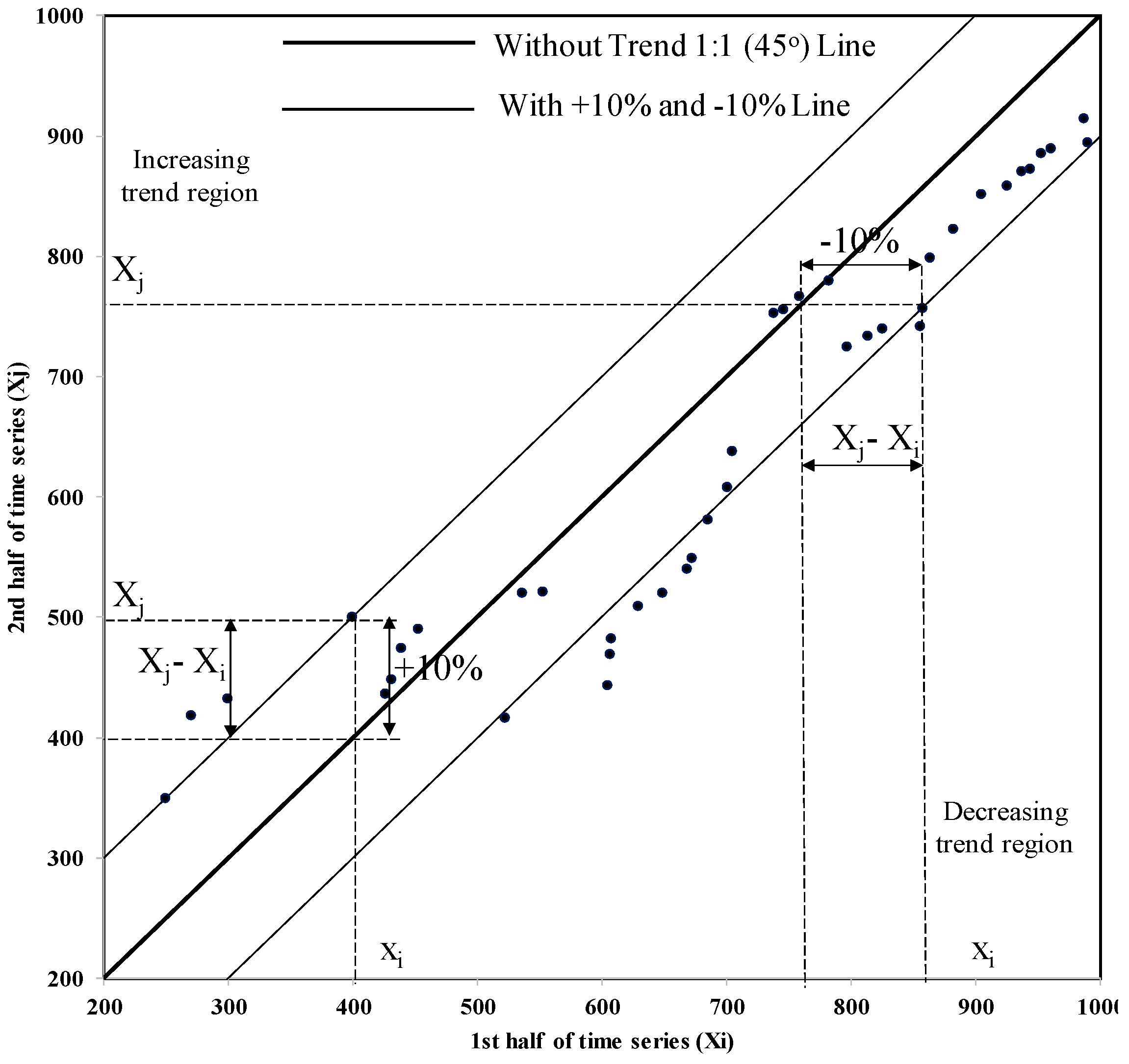
The innovative trend analysis method (Hereafter IM) (Figure 2) was recently developed and used to detect trends in a hydrometeorological time series [19]. The IM method is quite simple as compared to the Mann-Kendall test. The main steps involved in the IM method is as follows:

(1)

Dividing the selected hydrometeorological time series ($x=x_1,x_2,x_3,\dots \dots \dots ,x_n$) into two equal halves (i.e., $x_i=x_1,x_2,x_3,\dots \dots \dots ,x_{n/2}$ and $x_j=x_{\left(1+n/2\right)},x_{2+n/2},x_{3+n/2},\dots \dots \dots ,x_n$).

(2)

Arranging the subclasses independently in an ascending order.

(3)

Then, by using ordered data, a 1:1 scatter plot was drawn by plotting the 1st half $x_1,x_2,x_3,\dots \dots \dots ,x_{n/2}$) on the x-axis and the 2nd half ($x_{\left(1+n/2\right)},x_{2+n/2},x_{3+n/2},\dots \dots \dots ,x_n$) on the y-axis.

(4)

A straight line 1:1 (45° line) was then drawn on the same graph.

(5)

If the scatter data points lie below (above) the straight line, i.e., 1:1 (45° line), then there will be a decreasing (increasing) trend in the selected hydrometeorological time series. Similarly, if all the data points lie on the straight line, then no trend exists in the time series.

(6)

The trend magnitude (hereafter ITA) in a time series could be estimated by the average difference between two halves as given below:

$$ITA=\frac{1}{n}{\displaystyle \sum _{i=1}^n\frac{10\left(x_j-x_i\right)}{\overline{x}}}$$

(6)

where ITA = trend indicator, n = total number of the data point in subseries, $x_j$ = second half time series, $x_i$ represents 1st half time series, $\overline{x}$ is average of time series in the 1st half and ten is multiplied to the indicator to scale the matching and direct comparison with the MK test [19]. A positive ITA shows an increasing trend, whereas a negative ITA represents a decreasing trend.

2.3. Precipitation Variability Indices

The essential characteristics of the climatic variability of a region are the degree at which precipitation varies across the region or with time. To understand the precipitation variability, several indices have been used and analysed. Commonly used measures of variability in precipitation, e.g., standard deviation, could be interpreted for the manifestation of climate and weather analysis and to design specific local adaptation intrusion. In the current study, we used the consecutive disparity index (S), absolute inter-variability (IV) index and entropy-based variability index (D). The details are as follows:

2.3.1. Consecutive Disparity Index (S)

S is a variability index, generally used to assess internal variability in a highly irregular data series [45]. S is calculated as

$$S=\frac{1}{n-1}{\displaystyle \sum _{i=1}^{n-1}\left|\ln \left(\frac{P_{i+1}}{P_i}\right)\right|}$$

(7)

where $P_i$ and $P_{i+1}$ is the value of a variable at a time interval $i$ and $i+1$, and n is the length of series.

A constant K is added to the time series to evade any kind of indeterminate numerical (division with a negative value or zero):

$$S=\frac{1}{n-1}{\displaystyle \sum _{i=1}^{n-1}\left|\ln \left(\frac{P_{i+1}+k}{P_i+k}\right)\right|}$$

(8)

2.3.2. Absolute Inter-Variability (IV) Index

The IV index is a representation of the absolute measures of variability and mean absolute inter-variability [22] and calculated as given by

$$MAV=\frac{1}{N-1}\left({\displaystyle \sum _{i=1}^N\left|P_i-P_{i-1}\right|}\right)$$

(9)

$$IV=\frac{MAV}{\overline{P}}$$

(10)

2.3.3. Entropy-Based Variability Index (D)

The entropy theory [46] and maximum entropy principle [47] have been mostly used in environmental and hydrological studies. It is the measure of the disorder, dispersion, diversification and uncertainty of the variables to be considered.

Here in this study, the entropy-based variability index [48] has been used for assessment of spatiotemporal variability of precipitation and formalized as follows:

$$E_i=-{\displaystyle \sum _{i=1}^n{P}_i\ln \left(P_i\right)}$$

(11)

For average annual

$$\overline{E}=\frac{1}{n}{\displaystyle \sum _{i=1}^n{E}_i}$$

(12)

Variability is defined as the difference between maximum possible entropy and the entropy obtained by calculation from individual series. It is expressed by the disorder index

$$D_i={\log }_{2}n-E_i$$

(13)

The higher the value of the disorder index, the higher the precipitation variability. To compare the spatiotemporal variability, the mean value of the index was calculated as follows:

$$\overline{D}=\frac{1}{m}{\displaystyle \sum _{i=1}^m{D}_i}$$

(14)

3. Results and Discussions

3.1. Spatiotemporal Variation in Rainfall Series

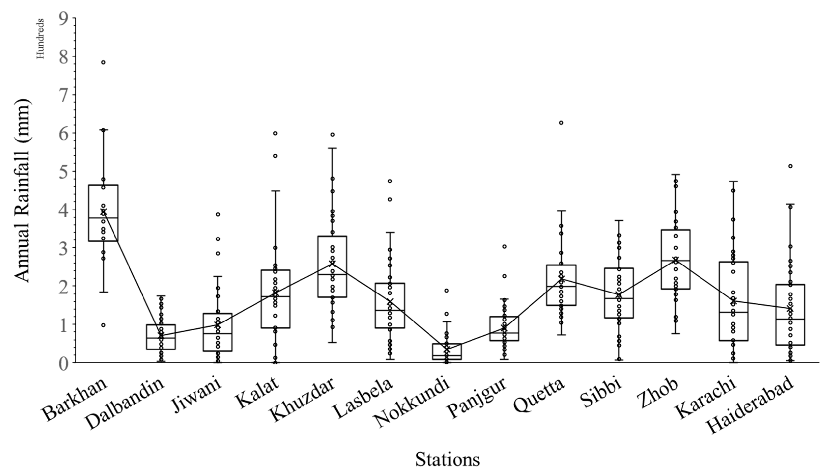
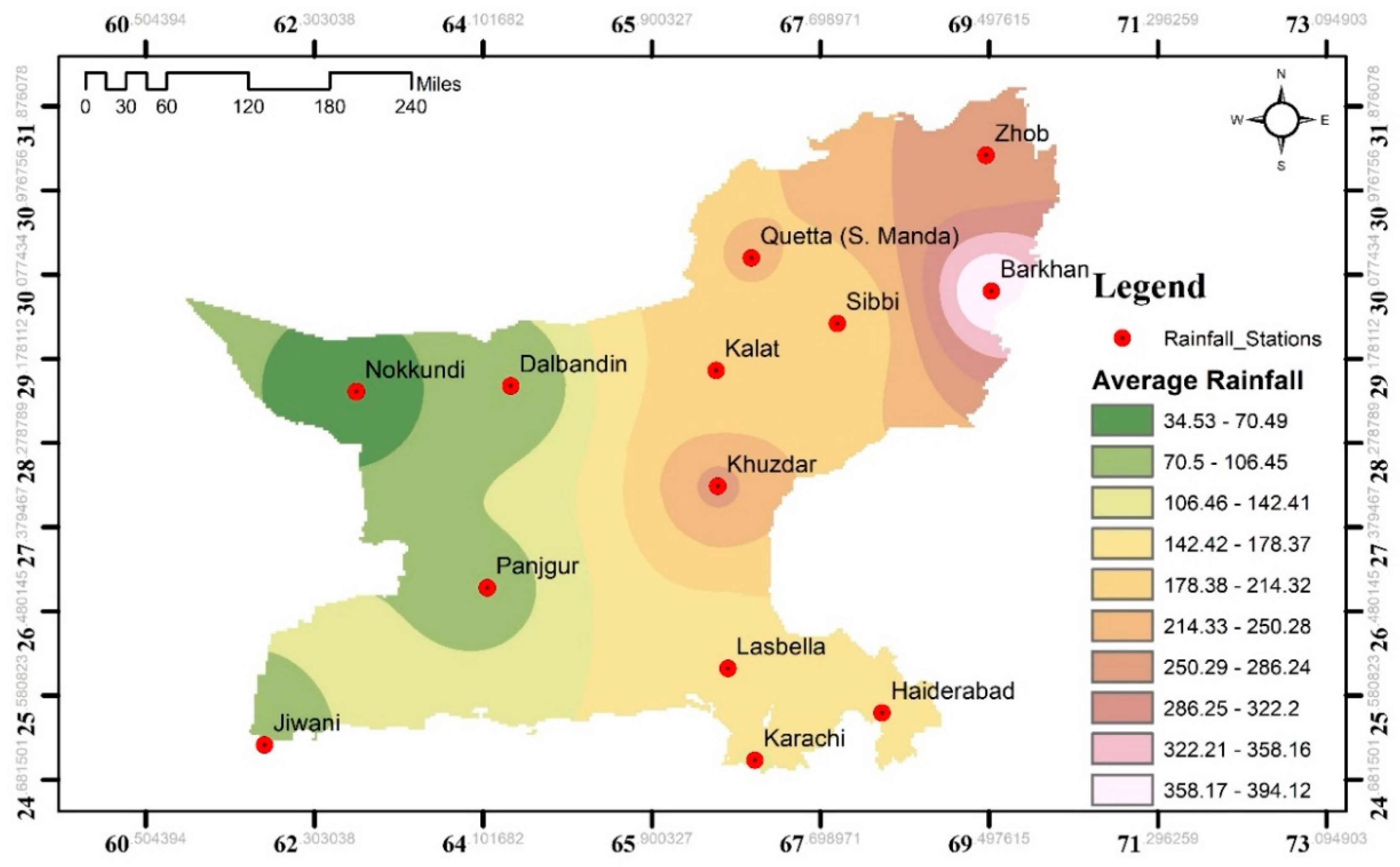
The annual spatiotemporal variation of precipitation at 13 stations in the southwest of Pakistan are shown in Figure 3 and Figure 4. The change in the annual time series was inconsistent at the selected stations as presented in Figure 3. It was expected, as the precipitation in the southwest region of Pakistan is generally influenced by western disturbances, monsoons and orographic effects (to an extent), and thus have a very complex and inconsistent behaviour regarding precipitation variation and distribution in the region [36,37,49]. However, in the sub-regions, a relative consistency was observed at different stations. For example, a relatively high precipitation was found in the eastern plateau of the region (including Barkhan, Zhob, Sibbi and Khuzdar) as compared to the west plateau (including Dalbadin, Nokkundi and Panjgur) and coastal region (Jiwani), as shown in Figure 3 and Figure 4. It was also noted that the precipitation goes on decreasing from the east plateau to the west plateau. It could be mainly due to the humid air coming from the Bay of Bengal entering the area from the southeast part and moisture in the air that goes on decreasing from east to west [36].

Keeping in view the average annual rainfall (Figure 3 and Figure 4), the selected stations were also regrouped into three subgroups, namely, G1, G2 and G3. Besides geographical grouping (eastern and west plateau and coastal area), these groups were also used to get more insight into the results. Barkhan, Zhob, Khuzdar, Kalat, Sibbi and Quetta were grouped as G1; Karachi, Haiderabad and Lasbella as G2; and Dalbadin, Nokkundi, Jiwani and Panjgur as G3.

3.2. Trend Analysis

3.2.1. Monthly Series Trends

The evaluation of the trend in the monthly precipitation series was carried out at each individual station, and the results are depicted in

Table 3. Results of Mann–Kendall test and IM approach statistic for monthly precipitation time series. (a) In case of MK: a rectangle means no significant trend, up-triangles indicate a significant increasing trend and down-triangles indicate a significant decreasing trend. (b) In case of ITA: an up-arrow, down-arrow and circle show a more than 10% decrease, more than 10% increase, and less than 10% increase/decrease, respectively.

. In the case of the MK test, a non-significant trend was observed in the majority of the cases, similar to [36,37], and in the case of May to August, a significant trend at the 5% significance level was also observed at most of the stations. It could be mainly because of the seasonal variation (discrete moisture transformation from the Bay of Bengal and the Arabian Sea) during summer and western disturbance [50]. Whereas, in the case of the ITA test, significant discrepancies in the results and direction of the trends were observed. Compared to MK, the ITA method showed that a considerable number of months had a more than 10% increasing or decreasing trend, except for March. The comparative analysis on a monthly basis revealed a 40% discrepancy in results between the two methods, where the opposite trend has been observed by the methods. The distinction between the two methods would be because of inherited restrictive assumption in the MK test [41] and sensitivity to outliers [19].

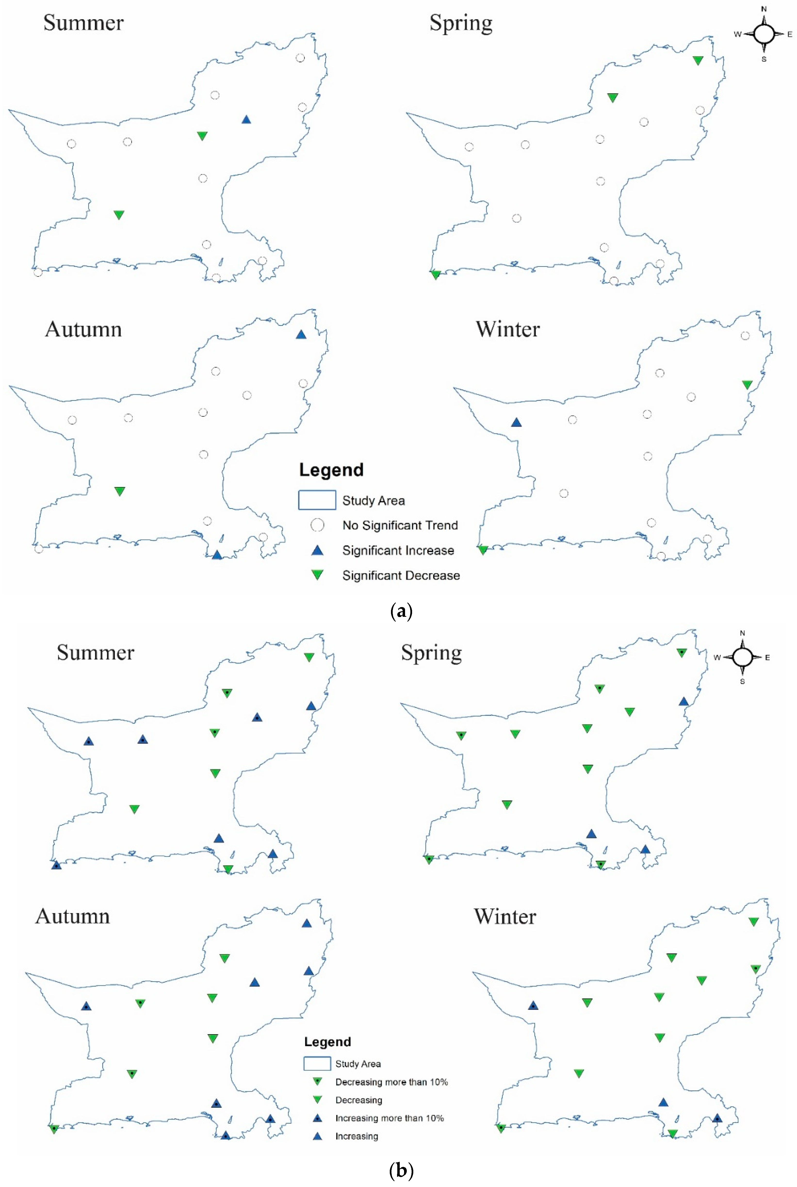
3.2.2. Seasonal Series Trends

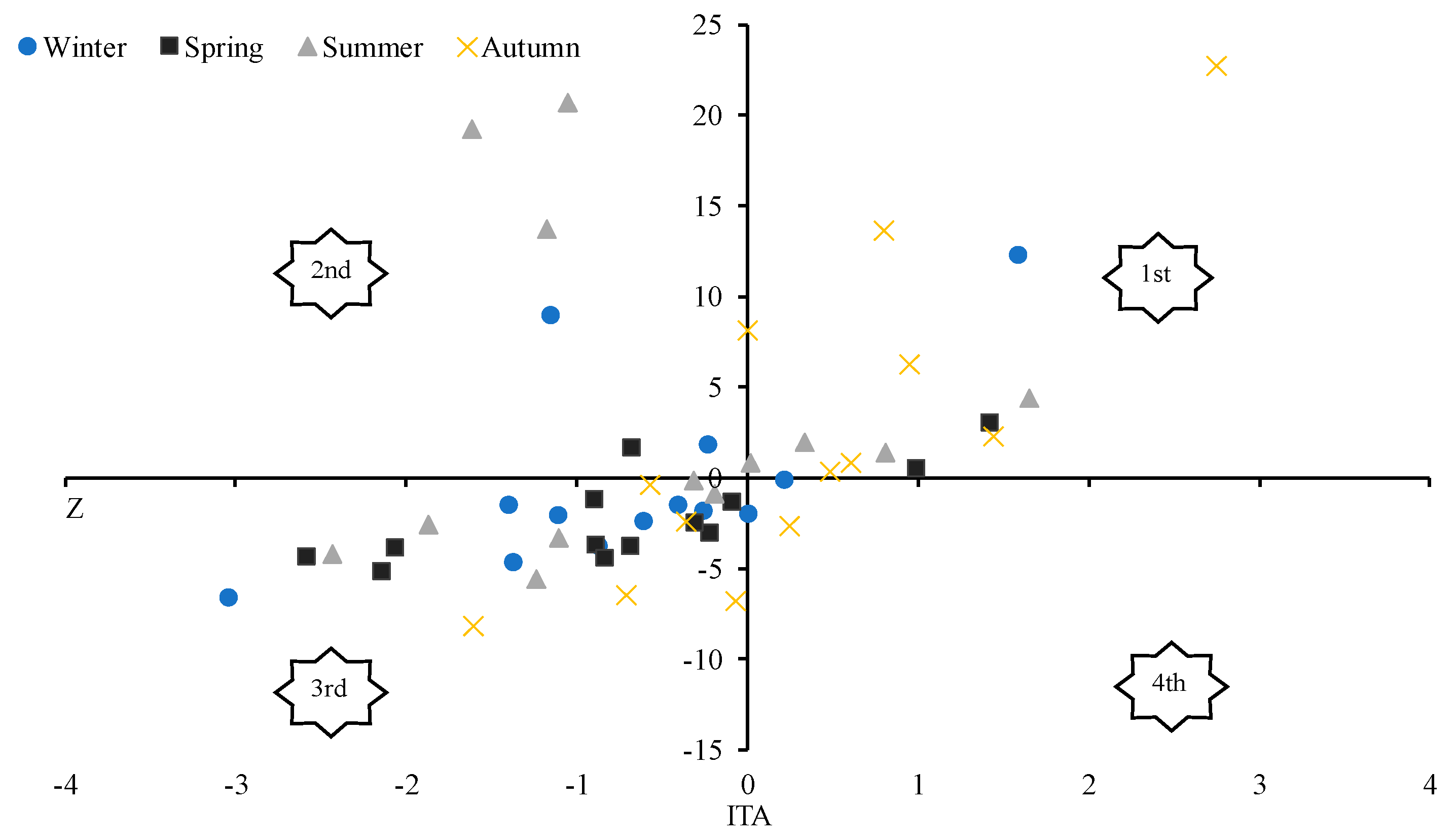
There are four seasons in Pakistan, namely, winter (from December to February), spring (from March to May), summer/monsoon period (from June to September) and autumn (from October to November). Considering the above mentioned four seasons, seasonal precipitation trends in the southwest arid region of Pakistan are observed using the same methods (Mann–Kendall and IM method), and results are shown in Figure 5a,b, respectively. In the case of Z, no significant trend was observed in all four seasons except for two or three discrete stations. However, compared to the average decreasing trend in winter at all of the stations, an increasing trend in spring and an inconsistency (a mixture of increasing and decreasing trend) resulted during summer and autumn. On the hand, there was a decreasing trend for winter, while an inconsistent trend for spring, summer and autumn were observed in the case of ITA. It will be noteworthy here to mention that at individual stations, a lot of discrepancies have been found between the two methods, especially in the case of summer and autumn. Figure 6 shows the scatter plot between Z versus ITA to indicate a general agreement in the trend in all methods in all seasons. The results indicated that for spring and winter seasons most of the points are in the 1st and 3rd coordinate, while discrepancies were noted in the case of summer.

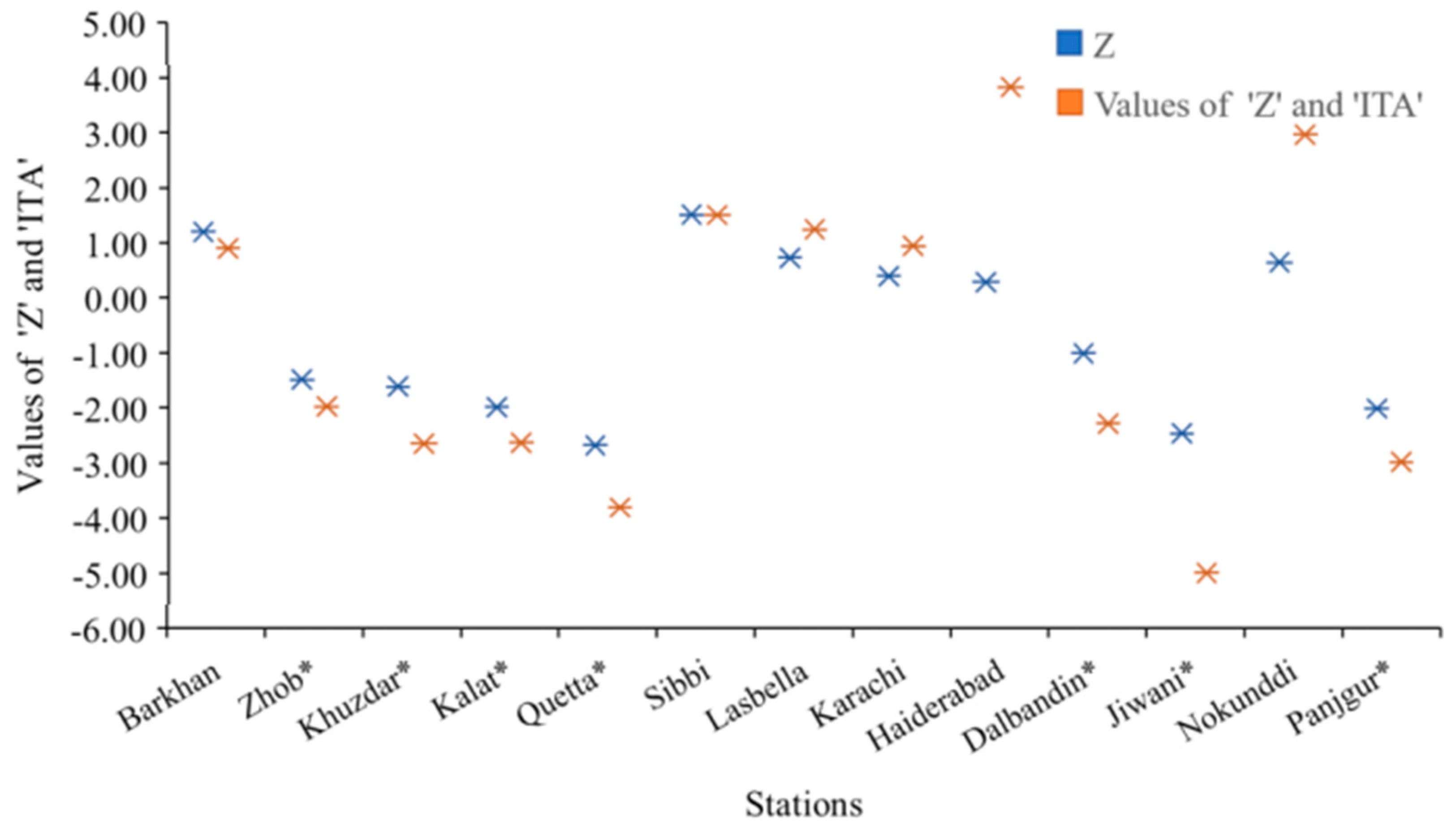
3.2.3. Annual Series Trends

Using an annual precipitation series, the results of the trend analysis are shown in Figure 7. It is evident from the results that in case of both tests, seven stations (with asterisk symbols) out of the eleven station show a decreasing trend direction, while the rest of the stations exhibit an increasing trend direction. It was also observed that only four stations exhibit a statistically significant trend in the case of the Mk test. Moreover, at most of the stations, both methods showed similar results (either increasing or decreasing) with a different amount/intensity. It was also noted that based on the annual time series, the stations in the east plateau, e.g., Barkhan, Khuzdar and Sibi, showed an increasing trend direction for precipitation (except Zhob), while the stations in the west plateau showed a decreasing trend similar to the coastal station. In addition to that, it was found that stations with a higher average rainfall (G1) have a negative trend, G2 (medium average rainfall) have a positive trend and G3 (low average rainfall) have a negative trend, except for Barkhan and Nokunddi. The inconsistency was expected due to the complex terrain and precipitation variability over a small distance [36,37,49].

3.3. Precipitation Variability

A better understanding of the irregular pattern of precipitation in a region could be gained through estimating the absolute variability indices, specifically, assessment of the temporal variation in precipitation. The precipitation variability based on entropy (D), consecutive variation (S) and inter variability (IV) has been assessed. Monthly time series analysis showed an on average higher variability in December, January, February and March for Nokkundi, Jiwani and Dalbandin, while in the case of Barkhan, Khuzdar and Zhob, July, August and September showed a comparatively high value of D, S and IV index values (note: results on a monthly basis are not shown here).

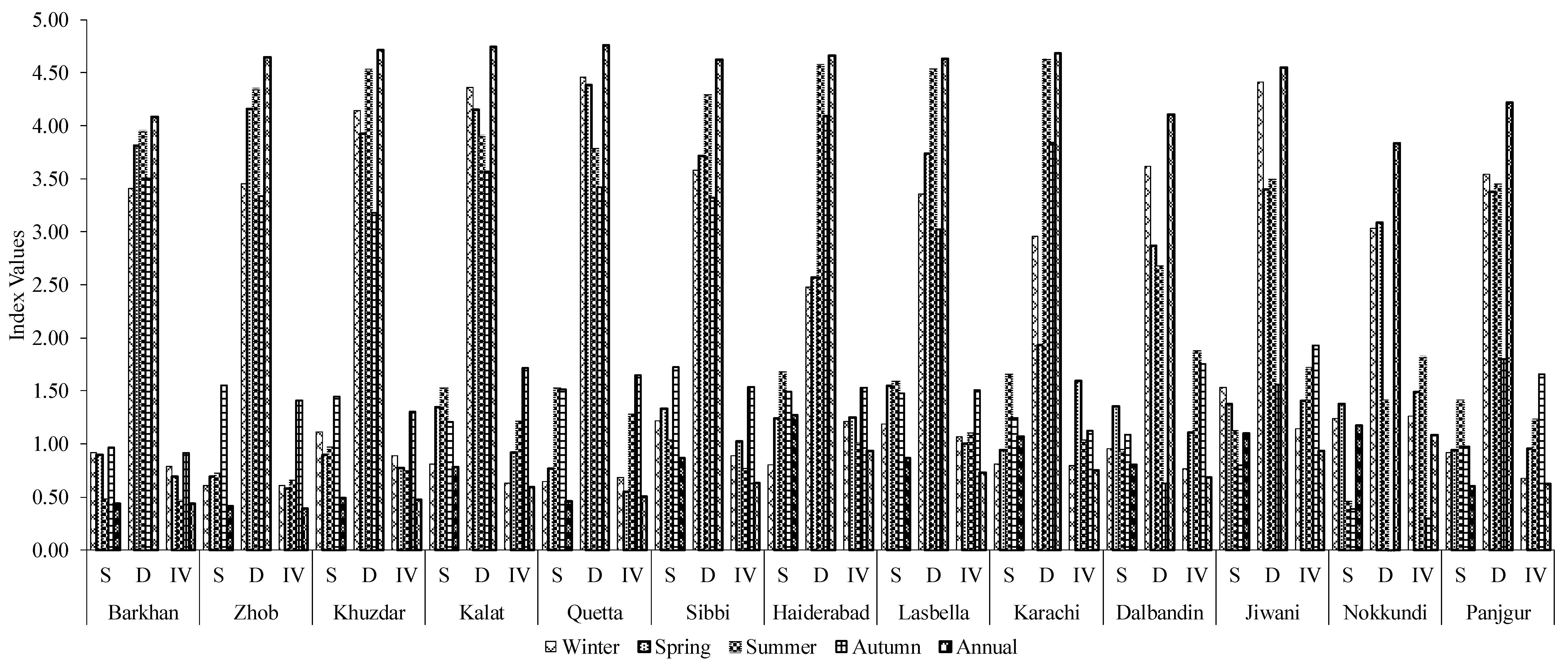
The results of selected indices for different seasons and on an annual basis are as shown in Figure 8. When comparing based on D, it shows that significant variability was observed on an annual basis and summer season shows more significant precipitation variability with an average D = 3.85, compared to other seasons. It was expected as the annual variation in the rainfall in the selected area of study is mainly affected by the monsoon season and movement of the moist air in the summer season. Hence, as precipitation variation in summer is high, variability is significantly higher in the summer season and on an annual basis. It was also observed that on an average the west plateau ensued a higher value of D (4.58) on an annual basis as compared to the east plateau with D = 4.08. Since the value of D could be affected by any unusual precipitation event, and the west plateau generally received such kind of precipitation event [36,37,49], the variation is comparatively high. It will be noteworthy here to mention that in the current study we used a different value of constant for different time series with a similar proportion of each time series, i.e., 1% of the average time series and a de-trending data series was used for the calculation of D.

Similarly, comparative analysis in the case of the S statistical index showed that on an average Nokunddi, Jiwani and Dalbandin show less consecutive intra variability among the individual season as this station lies in the western part, which is less affected by the moist air circulations. It was also noted that the autumn season followed by the summer season resulted in comparatively higher consecutive variability (S) at all selected stations with an average value of >1, whereas the winter season followed by the spring season showed an average value of S < 1. The results are summarised in Figure 8. On the other hand, results based on the IV index resulted in an average value of 0.88, 1.02, 1.15, 1.53 and 0.72 for winter, spring, summer, autumn and annual basis. It was observed that the inter-variability of the autumn season followed by summer was less compared to spring and winter. The results also second the outcome of variability index S. The observed variation in summer and autumn is in good agreement with the discrete mode of summer monsoonal rainfall [36,51,52].

3.4. Interrelationship between Approaches on a Seasonal and Annual Basis

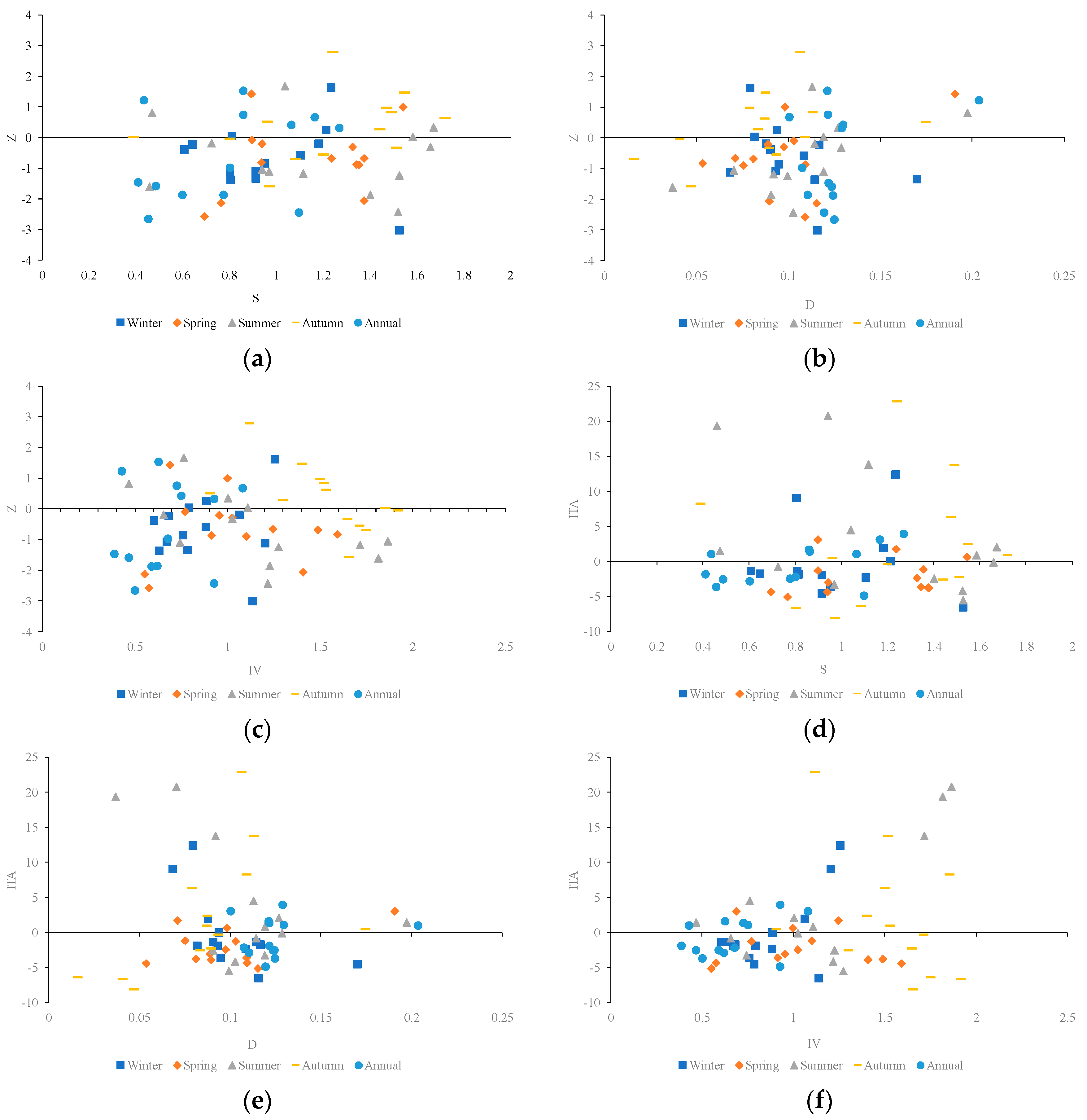
The results depicted above indicated that in the selected study area, precipitation dynamics are highly dependent upon the geographical patches and intensity. The discrepancies regarding trend direction and statistic values have been found in the outcomes of selected approaches. To better understand the interrelationship between different approaches used in the current study, an XY scatter plot representation was used, and the results are shown in Figure 9. The results in Figure 9 are indicating the relationship between the seasonal and annual values of the trend analysis method (Z and ITA) and variability indices (S, D and IV) at each station. From the Figure 9a–f scatter plots, it was observed that the variability indices show a better agreement with the ITA method compared to the Mann–Kendall method. It was also noted that the statistical index D have a better agreement in case of spring, winter and summer, while statistical index P have a better correlation for the autumn season. In addition, the correlation analysis based on groups (G1, G2 and G3) resulted that the trend statistics have a higher correlation with statistical indices the in case of stations in G2, while comparatively low agreement in case of stations in G1 and G3.

4. Conclusions

Finally, the following conclusion was drawn from the current study: (1) In most of the cases, the seasonal time series seemingly have a more significant trend variation as compared to the annual time series (masking the effect of distinct months). The seasons contribute differently to the annual precipitation variation. The winter season was showing a decreasing trend, while mixtures of increasing and decreasing trends were found during spring, summer and autumn. (2) The study signposted that, on average, an increasing trend direction was observed in the eastern plateau and decreasing in the west plateau. (3) The spatial variation also resulted in differences for different seasons. On an average, summer seasons seem to have more significant variability. (4) No systematic precipitation pattern across the study region was observed in monthly, annual and seasonal time series. (5) The precipitation variability analysis resulted in higher variability in the case of the east plateau, while lower for the west plateau at all seasonal and annual basis. Moreover, no systematic agreement was found in the inter/intra relationship between trend detection methods and absolute indices, which could be further evaluated. (6) The results also indicated the low availability of water resources in the west plateau and the need for the use of water within constraint. (7) The overall results signposted that, on average, seven out of eleven stations showed a decreasing trend in precipitation. As the livelihood and economy of the region are mainly dependent on the precipitation as a major water source, any kind of imbalance or decline in precipitation could result in depletion of water resources, aridity, periodic drought and degraded rangelands. This also means that agriculture could need more artificial application of water, which is already limited in this region, and proper adaptation strategies (e.g., irrigation management, soil moisture conservation techniques, selection of resilient crops, planting dates variation, suitable cropping intensities, pattern change and index insurance) would be necessary to cope with the possible impacts of climate change.

References

- Adler, R.F.; Huffman, G.J.; Bolvin, D.T.; Curtis, S.; Nelkin, E.J. Tropical rainfall distributions determined using TRMM combined with other satellite and rain gauge information. J. Appl. Meteorol. 2000, 39, 2007–2023. [Google Scholar] [CrossRef] [Green Version]
- Banadkooki, F.B.; Ehteram, M.; Ahmed, A.N.; Fai, C.M.; Afan, H.A.; Ridwam, W.M.; Sefelnasr, A.; El-Shafie, A. Precipitation forecasting using multilayer neural network and support vector machine optimization based on flow regime algorithm taking into account uncertainties of soft computing models. Sustainability 2019, 11, 6681. [Google Scholar] [CrossRef] [Green Version]
- Eshetu, G.; Johansson, T.; Garedew, W. Rainfall trend and variability analysis in setema-gatira area of Jimma, southwestern Ethiopia. Afr. J. Agric. Res. 2016, 11, 3037–3045. [Google Scholar]
- Begum, M.A.R.M. Application of non-parametric test for trend detection of rainfall in the largest island of Bangladesh. ARPN J.Earth Sci. 2006, 2, 40–44. [Google Scholar]
- Khan, N.; Shahid, S.; Ahmed, K.; Ismail, T.; Nawaz, N.; Son, M. Performance assessment of general circulation model in simulating daily precipitation and temperature using multiple gridded datasets. Water 2018, 10, 1793. [Google Scholar] [CrossRef] [Green Version]
- Longobardi, A.; Villani, P. Trend analysis of annual and seasonal rainfall time series in the Mediterranean area. Int. J. Climatol. 2010, 30, 1538–1546. [Google Scholar] [CrossRef]
- Ambun, D.; Azlai, B.; Phuah, E. Statistical and trend analysis of rainfall data in Kuching, Sarawak from 1968–2010. Res. Publ. 2013, 6, 17. [Google Scholar]
- Kansiime, M.K.; Wambugu, S.K.; Shisanya, C.A. Perceived and actual rainfall trends and variability in eastern Uganda: Implications for community preparedness and response. J. Nat. Sci. Res. 2013, 3, 179–194. [Google Scholar]
- Nyatuame, M.; Owusu-Gyimah, V.; Ampiaw, F. Statistical analysis of rainfall trend for Volta region in Ghana. Int. J. Atmos. Sci. 2014, 2014. [Google Scholar] [CrossRef] [Green Version]
- Piao, S.; Ciais, P.; Huang, Y.; Shen, Z.; Peng, S.; Li, J.; Zhou, L.; Liu, H.; Ma, Y.; Ding, Y. The impacts of climate change on water resources and agriculture in China. Nature 2010, 467, 43–51. [Google Scholar] [CrossRef]
- Gocic, M.; Trajkovic, S. Analysis of precipitation and drought data in Serbia over the period 1980–2010. J. Hydrol. 2013, 494, 32–42. [Google Scholar] [CrossRef]
- Manly, B.F.; Mackenzie, D. A cumulative sum type of method for environmental monitoring. Environmetrics 2000, 11, 151–166. [Google Scholar] [CrossRef]
- Westra, S.; Alexander, L.V.; Zwiers, F.W. Global increasing trends in annual maximum daily precipitation. J. Clim. 2013, 26, 3904–3918. [Google Scholar] [CrossRef] [Green Version]
- Haktanir, T.; Citakoglu, H. Trend, independence, stationarity, and homogeneity tests on maximum rainfall series of standard durations recorded in Turkey. J. Hydrol. Eng. 2014, 19, 05014009. [Google Scholar] [CrossRef]
- Shadmani, M.; Marofi, S.; Roknian, M. Trend analysis in reference evapotranspiration using Mann-Kendall and spearman’s rho tests in arid regions of Iran. Water Resour. Manag. 2012, 26, 211–224. [Google Scholar] [CrossRef] [Green Version]
- Yue, S.; Wang, C.Y. Applicability of prewhitening to eliminate the influence of serial correlation on the Mann-Kendall test. Water Resour. Res. 2002, 38, 4-1–4-7. [Google Scholar] [CrossRef]
- Zhang, X.-L.; Wang, S.-J.; Zhang, J.-M.; Wang, G.; Tang, X.-Y. Temporal and spatial variability in precipitation trends in the southeast Tibetan plateau during 1961–2012. Clim. Past Discuss. 2015, 11, 447–487. [Google Scholar] [CrossRef] [Green Version]
- Zhao, J.; Huang, Q.; Chang, J.; Liu, D.; Huang, S.; Shi, X. Analysis of temporal and spatial trends of hydro-climatic variables in the Wei river basin. Environ. Res. 2015, 139, 55–64. [Google Scholar] [CrossRef]
- Wu, H.; Qian, H. Innovative trend analysis of annual and seasonal rainfall and extreme values in Shaanxi, China, since the 1950s. Int. J. Climatol. 2017, 37, 2582–2592. [Google Scholar] [CrossRef]
- Markus, M.; Demissie, M.; Short, M.B.; Verma, S.; Cooke, R.A. Sensitivity analysis of annual nitrate loads and the corresponding trends in the lower Illinois river. J. Hydrol. Eng. 2014, 19, 533–543. [Google Scholar] [CrossRef]
- Zahid, M.; Rasul, G. Frequency of extreme temperature and precipitation events in Pakistan 1965–2009. Sci. Int. 2011, 23, 313–319. [Google Scholar]
- Wani, J.M.; Sarda, V.; Jain, S.K. Assessment of trends and variability of rainfall and temperature for the district of mandi in Himachal Pradesh, India. Slovak J. Civ. Eng. 2017, 25, 15–22. [Google Scholar] [CrossRef] [Green Version]
- Hartmann, H.; Andresky, L. Flooding in the Indus river basin—A spatiotemporal analysis of precipitation records. Glob. Planet. Chang. 2013, 107, 25–35. [Google Scholar] [CrossRef]
- Abbas, F. Analysis of a historical (1981–2010) temperature record of the Punjab province of Pakistan. Earth Interact. 2013, 17, 1–23. [Google Scholar] [CrossRef]
- Adnan, S.; Ullah, K.; Gao, S.; Khosa, A.H.; Wang, Z. Shifting of agro-climatic zones, their drought vulnerability, and precipitation and temperature trends in Pakistan. Int. J. Climatol. 2017, 37, 529–543. [Google Scholar] [CrossRef]
- Ali, N.; Ahmad, I.; Chaudhry, A.G.; Raza, M.A. Trend analysis of precipitation data in Pakistan. Sci. Int. 2015, 27, 803–808. [Google Scholar]
- Bocchiola, D.; Diolaiuti, G. Recent (1980–2009) evidence of climate change in the upper Karakoram, Pakistan. Theor. Appl. Climatol. 2013, 113, 611–641. [Google Scholar] [CrossRef]
- Gadiwala, M.S.; Burke, F. Climate change and precipitation in Pakistan-a meteorological prospect. Int. J. Econ. Environ. Geol. 2019, 4, 10–15. [Google Scholar]
- Hanif, M.; Khan, A.H.; Adnan, S. Latitudinal precipitation characteristics and trends in Pakistan. J. Hydrol. 2013, 492, 266–272. [Google Scholar] [CrossRef]
- Hussain, M.S.; Lee, S. Long-term variability and changes of the precipitation regime in Pakistan. Asia Pac. J. Atmos. Sci. 2014, 50, 271–282. [Google Scholar] [CrossRef]
- Ahmad, I.; Tang, D.; Wang, T.; Wang, M.; Wagan, B. Precipitation trends over time using Mann-Kendall and spearman’s rho tests in swat river basin, Pakistan. Adv. Meteorol. 2015, 2015. [Google Scholar] [CrossRef] [Green Version]
- Iqbal, M.F.; Athar, H. Variability, trends, and teleconnections of observed precipitation over Pakistan. Theor. Appl. Climatol. 2018, 134, 613–632. [Google Scholar] [CrossRef]
- Latif, Y.; Yaoming, M.; Yaseen, M. Spatial analysis of precipitation time series over the upper Indus basin. Theor. Appl. Climatol. 2018, 131, 761–775. [Google Scholar] [CrossRef] [Green Version]
- Naheed, G.; Kazmi, D.; Rasul, G. Seasonal variation of rainy days in Pakistan. Pak. J. Meteorol. 2013, 9, 18. [Google Scholar]
- Raza, M.; Hussain, D.; Rasul, G. Climatic Variability and Linear Trend Models for the Six Major Regions of Gilgit-Baltistan Pakistan. B. Life Environ. Sci. 2016, 53, 129–136. [Google Scholar]
- Ahmed, K.; Shahid, S.; Ali, R.O.; Harun, S.; Wang, X. Evaluation of the performance of gridded precipitation products over Balochistan province, Pakistan. Desalination 2017, 1, 14. [Google Scholar] [CrossRef]
- Salma, S.; Shah, M.; Rehman, S. Rainfall trends in different climate zones of Pakistan. Pak. J. Meteorol. 2012, 9, 17. [Google Scholar]
- Ullah, S.; You, Q.; Ullah, W.; Ali, A. Observed changes in precipitation in China-Pakistan economic corridor during 1980–2016. Atmos. Res. 2018, 210, 1–14. [Google Scholar] [CrossRef]
- Krakauer, N.Y.; Lakhankar, T.; Dars, G.H. Precipitation trends over the Indus basin. Climate 2019, 7, 116. [Google Scholar] [CrossRef] [Green Version]
- Iqbal, Z.; Shahid, S.; Ahmed, K.; Ismail, T.; Nawaz, N. Spatial distribution of the trends in precipitation and precipitation extremes in the sub-Himalayan region of Pakistan. Theor. Appl. Climatol. 2019, 137, 2755–2769. [Google Scholar] [CrossRef]
- Ahmad, I.; Zhang, F.; Tayyab, M.; Anjum, M.N.; Zaman, M.; Liu, J.; Farid, H.U.; Saddique, Q. Spatiotemporal analysis of precipitation variability in annual, seasonal and extreme values over upper Indus river basin. Atmos. Res. 2018, 213, 346–360. [Google Scholar] [CrossRef]
- Mann, H.B. Nonparametric tests against trend. Econometrica 1945, 13, 245–259. [Google Scholar] [CrossRef]
- Pettitt, A.N. A simple cumulative sum type statistic for the change-point problem with zero-one observations. Biometrika 1980, 67, 79–84. [Google Scholar] [CrossRef]
- Zeng, Y.; Zhou, Z.; Yan, Z.; Teng, M.; Huang, C. Climate change and its attribution in three gorges reservoir area, China. Sustainability 2019, 11, 7206. [Google Scholar] [CrossRef] [Green Version]
- Fernández-Martínez, M.; Vicca, S.; Janssens, I.A.; Carnicer, J.; Martín-Vide, J.; Peñuelas, J. The consecutive disparity index, d: A measure of temporal variability in ecological studies. Ecosphere 2018, 9, e02527. [Google Scholar] [CrossRef] [Green Version]
- Shannon, C.E. A mathematical theory of communication. Bell Syst. Tech. J. 1948, 27, 379–423. [Google Scholar] [CrossRef] [Green Version]
- Jaynes, E.T. Information theory and statistical mechanics. Phys. Rev. 1957, 106, 620. [Google Scholar] [CrossRef]
- Zhao, C.; Ding, Y.; Ye, B.; Yao, S.; Zhao, Q.; Wang, Z.; Wang, Y. An analyses of long-term precipitation variability based on entropy over Xinjiang, northwestern China. Hydrol. Earth Syst. Sci. Discuss. 2011, 8, 2975–2999. [Google Scholar] [CrossRef]
- Aamir, E.; Hassan, I. Trend analysis in precipitation at individual and regional levels in Baluchistan, Pakistan. In IOP Conference Series: Materials Science and Engineering; IOP Publishing: Bristol, UK, 2018; p. 012042. [Google Scholar]
- Faiz, M.A.; Liu, D.; Fu, Q.; Wrzesiński, D.; Muneer, S.; Khan, M.I.; Li, T.; Cui, S. Assessment of precipitation variability and uncertainty of streamflow in the Hindu kush himalayan and Karakoram river basins of Pakistan. Meteorol. Atmos. Phys. 2019, 131, 127–136. [Google Scholar] [CrossRef]
- Hasson, S.; Böhner, J.; Lucarini, V. Prevailing climatic trends and runoff response from Hindukush–Karakoram–Himalaya, upper Indus basin. Earth Syst. Dyn. 2017, 8, 337–355. [Google Scholar] [CrossRef] [Green Version]
- Hasson, S.U.; Pascale, S.; Lucarini, V.; Böhner, J. Seasonal cycle of precipitation over major river basins in south and southeast Asia: A review of the CMIP5 climate models data for present climate and future climate projections. Atmos. Res. 2016, 180, 42–63. [Google Scholar] [CrossRef] [Green Version]
Figure 1.
Relative location of the study area and meteorological stations.
Figure 2.
A detailed description of the innovative trend analysis method (IM).
Figure 3.
Statistical summary (by box plot representation) of the annual rainfall at selected stations.
Figure 4.
Spatial variability of average annual rainfall over the southwest region of Pakistan.
Figure 5.
Results of seasonal trend analysis using (a) the Mann–Kendall and (b) the IM method.
Figure 6.
Scatter plotting between “Z” and “ITA”.
Figure 7.
Results of the Mann–Kendall test (Z) and IM approach statistic (ITA) for an annual precipitation time series. * decreasing trend.
Figure 8.
Results of precipitation variability at season scale using variability indices, i.e., the consecutive disparity index (S), entropy-based variability index (D) and absolute inter-variability (IV) index.
Figure 9.
Results of the interrelationship between trend detection methods (Z and ITA) and variability indices (S, D and IV) on a seasonal and annual basis. (a)—relationship between Z and S, (b)—relationship between Z and D, (c)—relationship between Z and IV, (d)—relationship between ITA and D, (e)—relationship between ITA and D, and (f)—relationship between ITA and IV.