Computation of Global and Local Mass Transfer in Hollow Fiber Membrane Modules

 , , , , and
Abstract
:1. Introduction
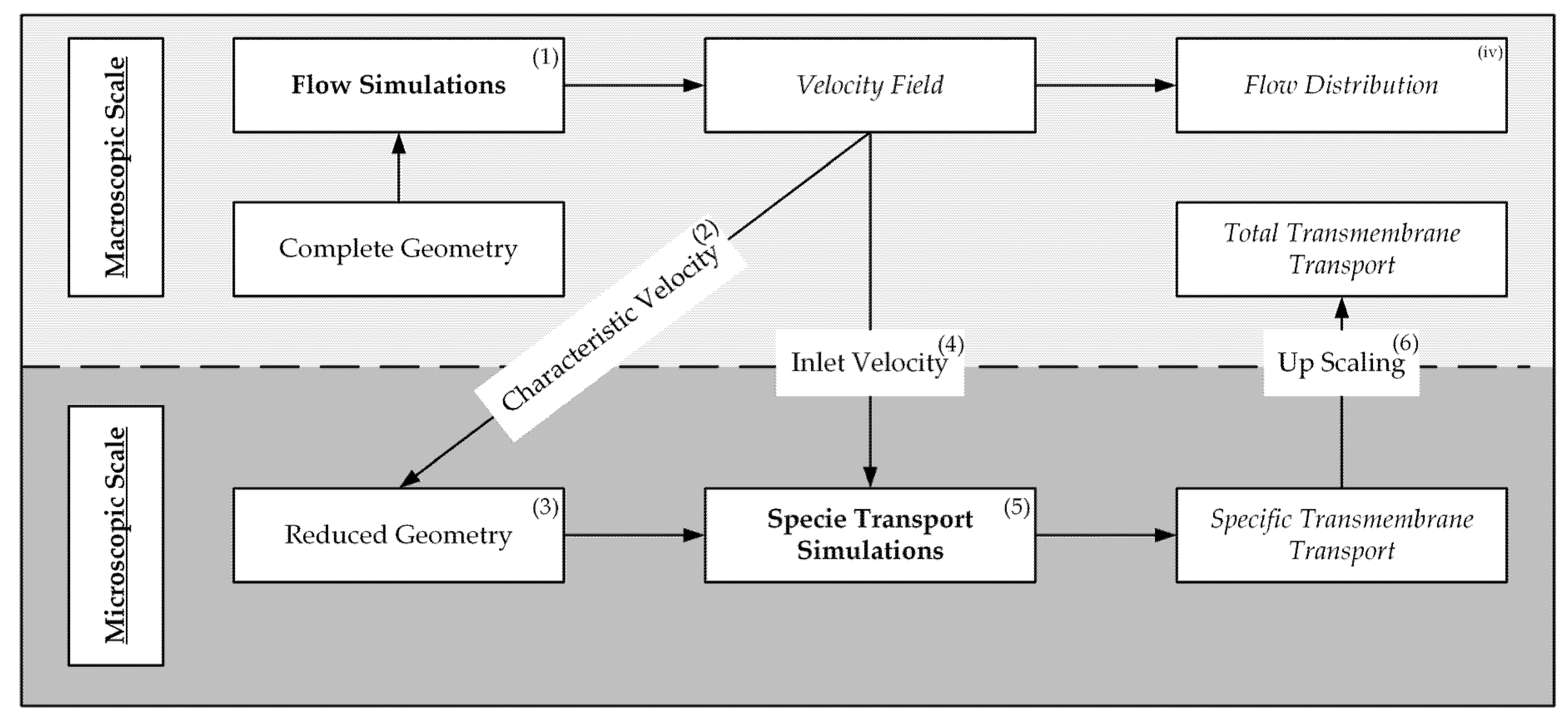
- Flow simulations for computation of the velocity field in the complete geometry,
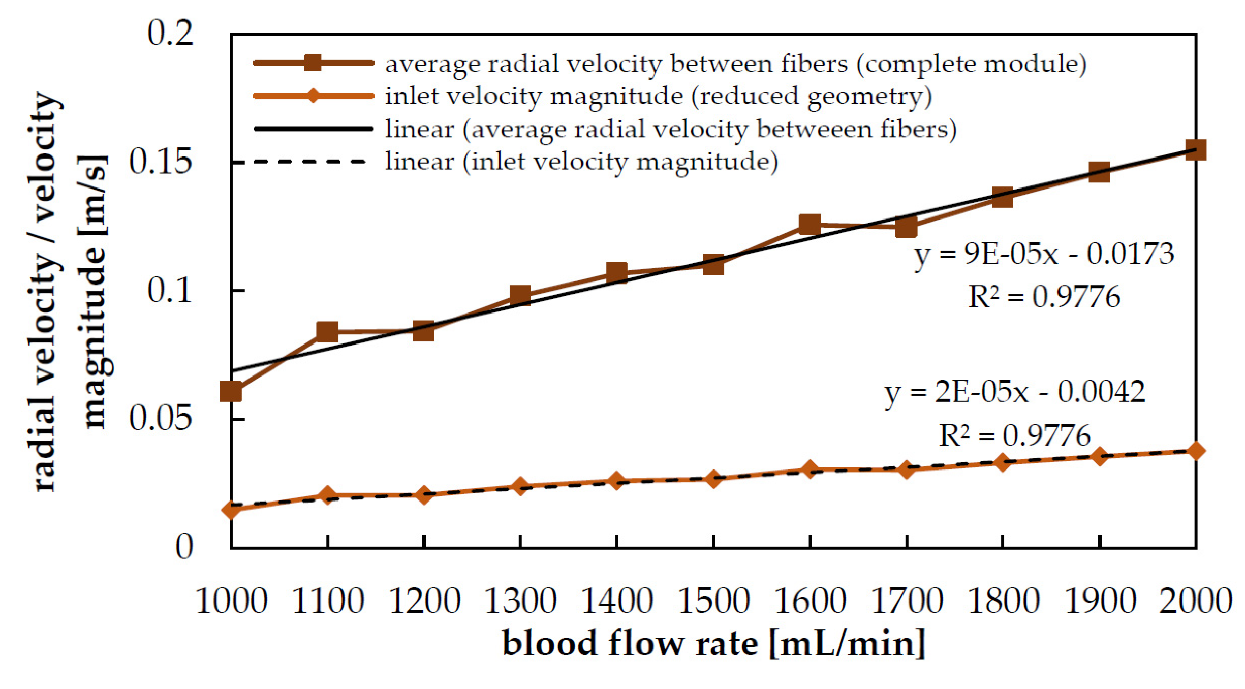
- Identification of characteristic velocity components with significant influence on the transmembrane species transport,
- Development of a reduced packing geometry based on the velocity distribution,
- Numerical conversion of the characteristic velocity to an inlet velocity for the reduced geometry,
- Species transport simulations of the reduced geometry to predict transmembrane flux,
- Upscaling of the transmembrane flux to predict the total transmembrane transport of the whole module.
2. Experimental and Numerical Methods
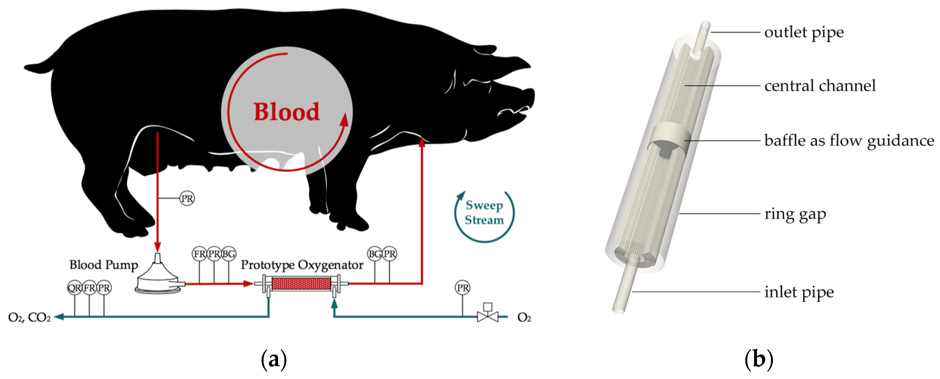
2.1. Ex Vivo Tests
2.2. Computational Fluid Dynamics
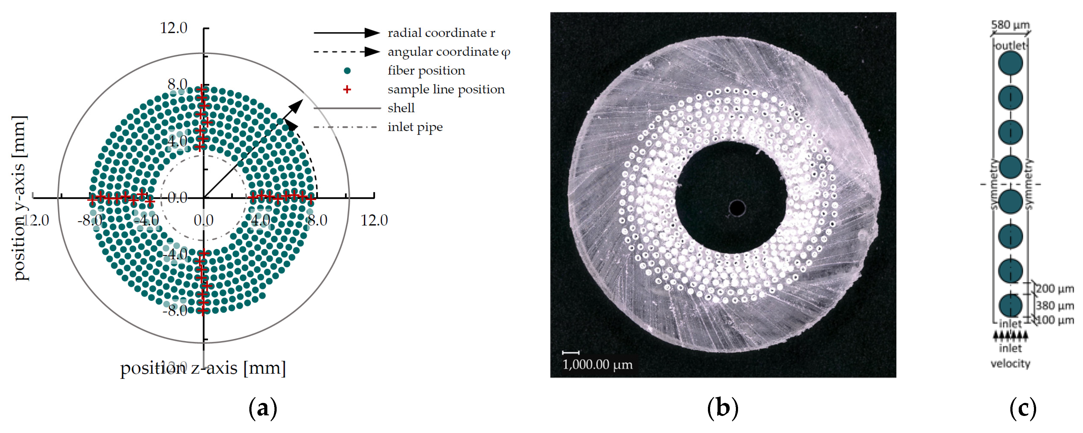
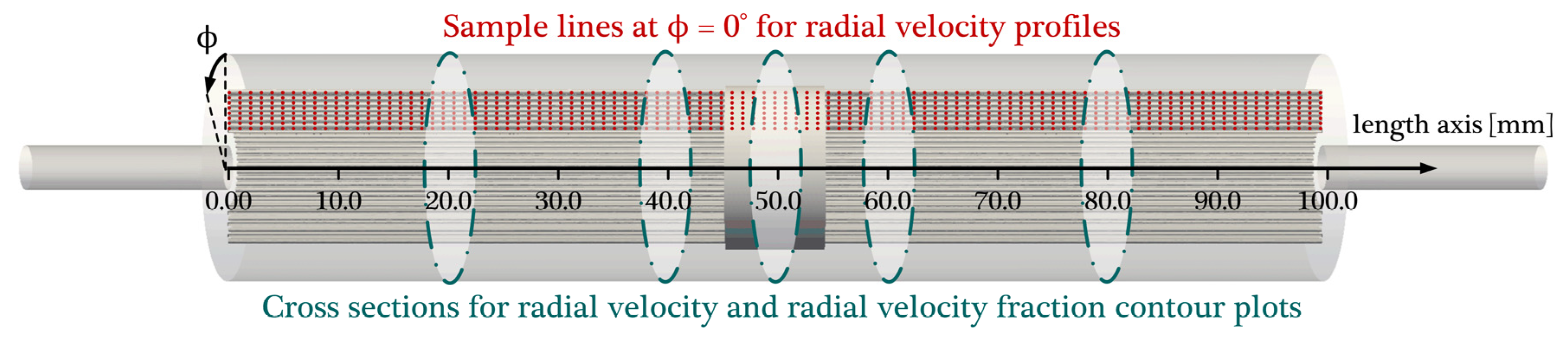
2.2.1. Flow Simulation of the Complete Membrane Module
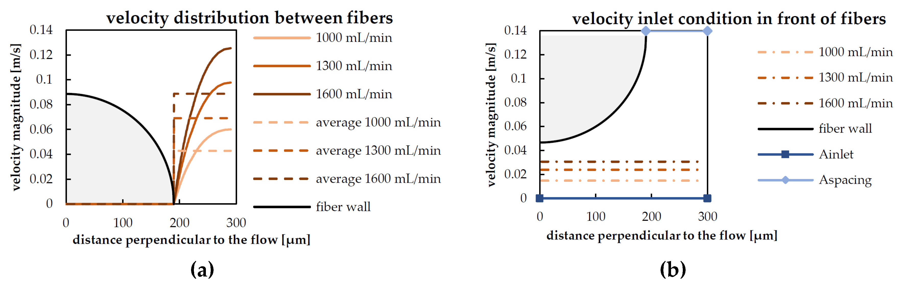
2.2.2. Derivation of the Reduced Geometry, Computation of Inlet Velocities
2.2.3. Species Transport Simulations of the Reduced Geometry
3. Results and Discussion
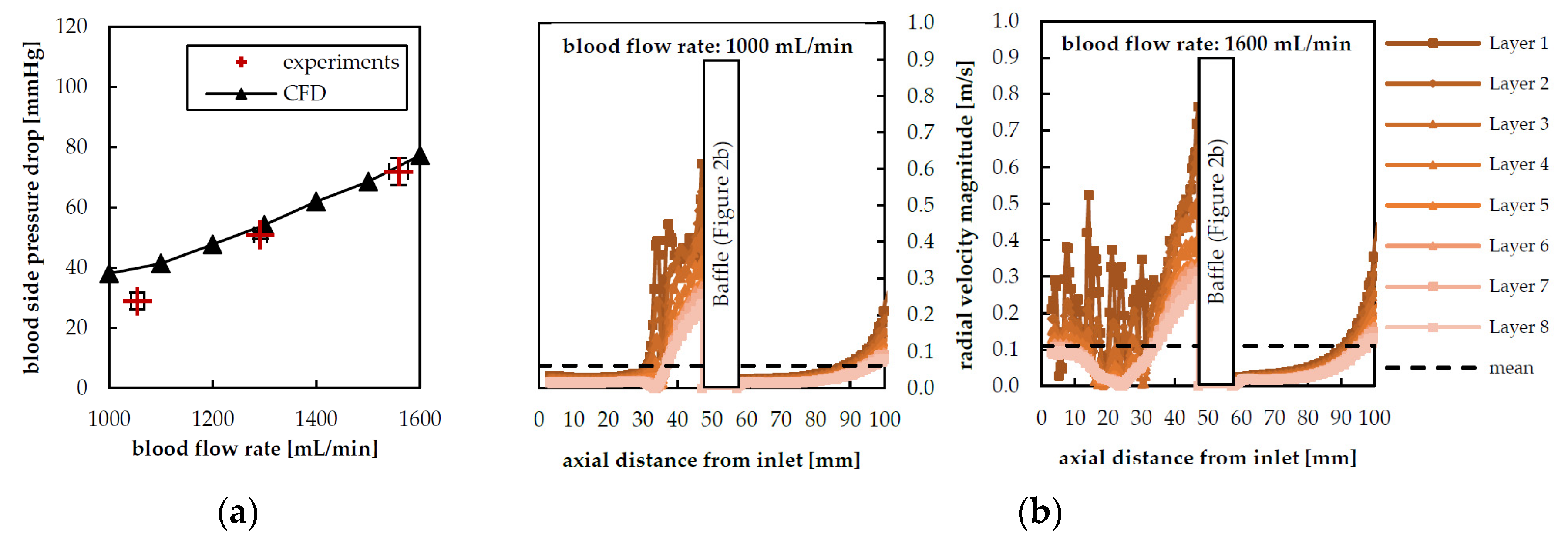
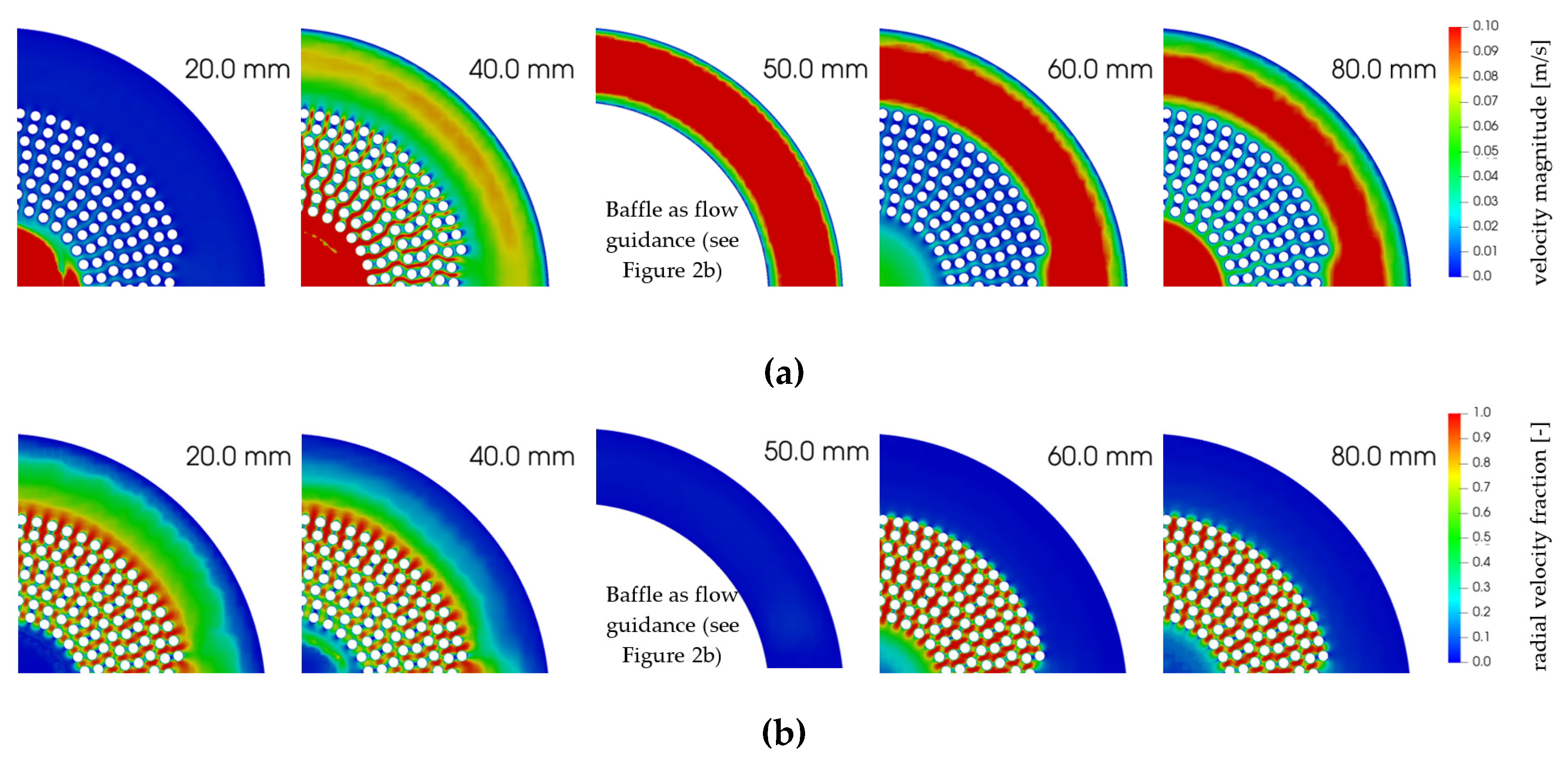
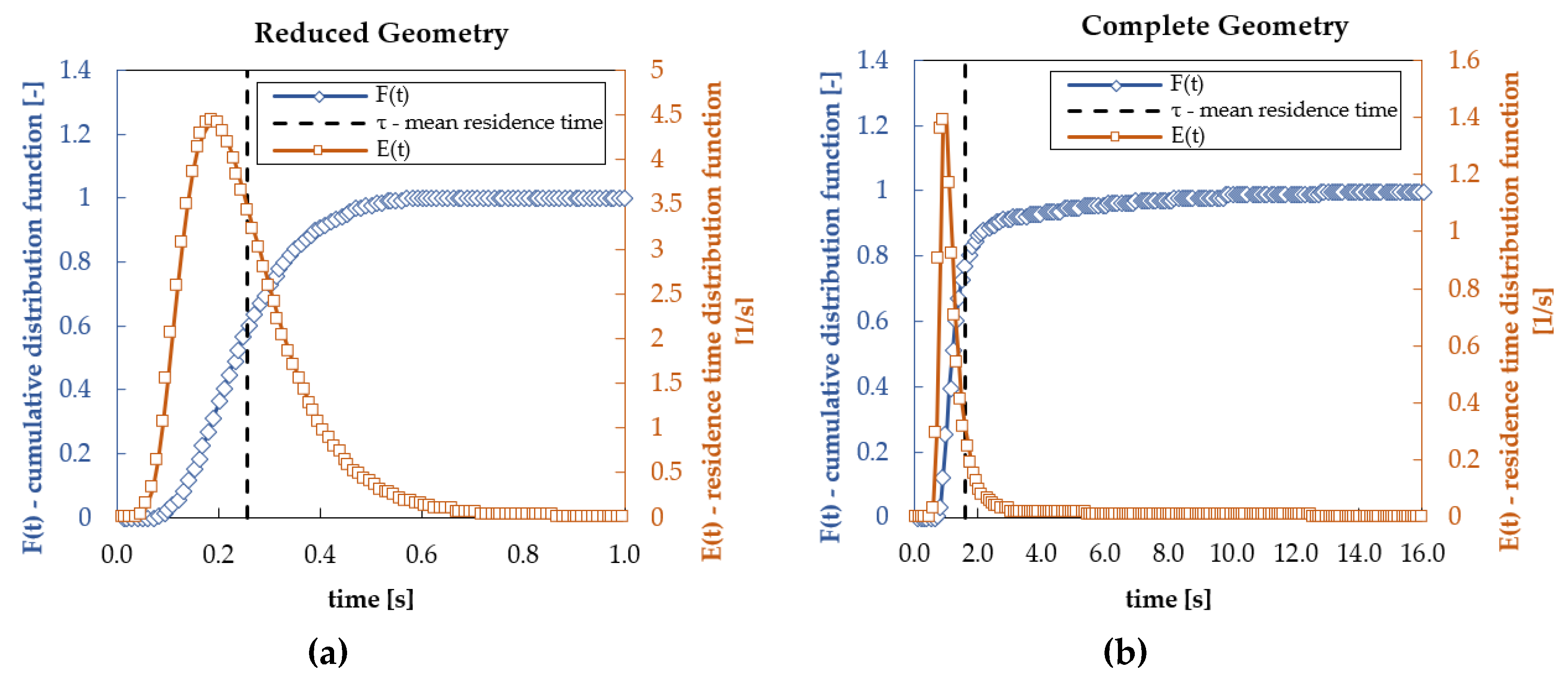
3.1. Hydrodynamic Results
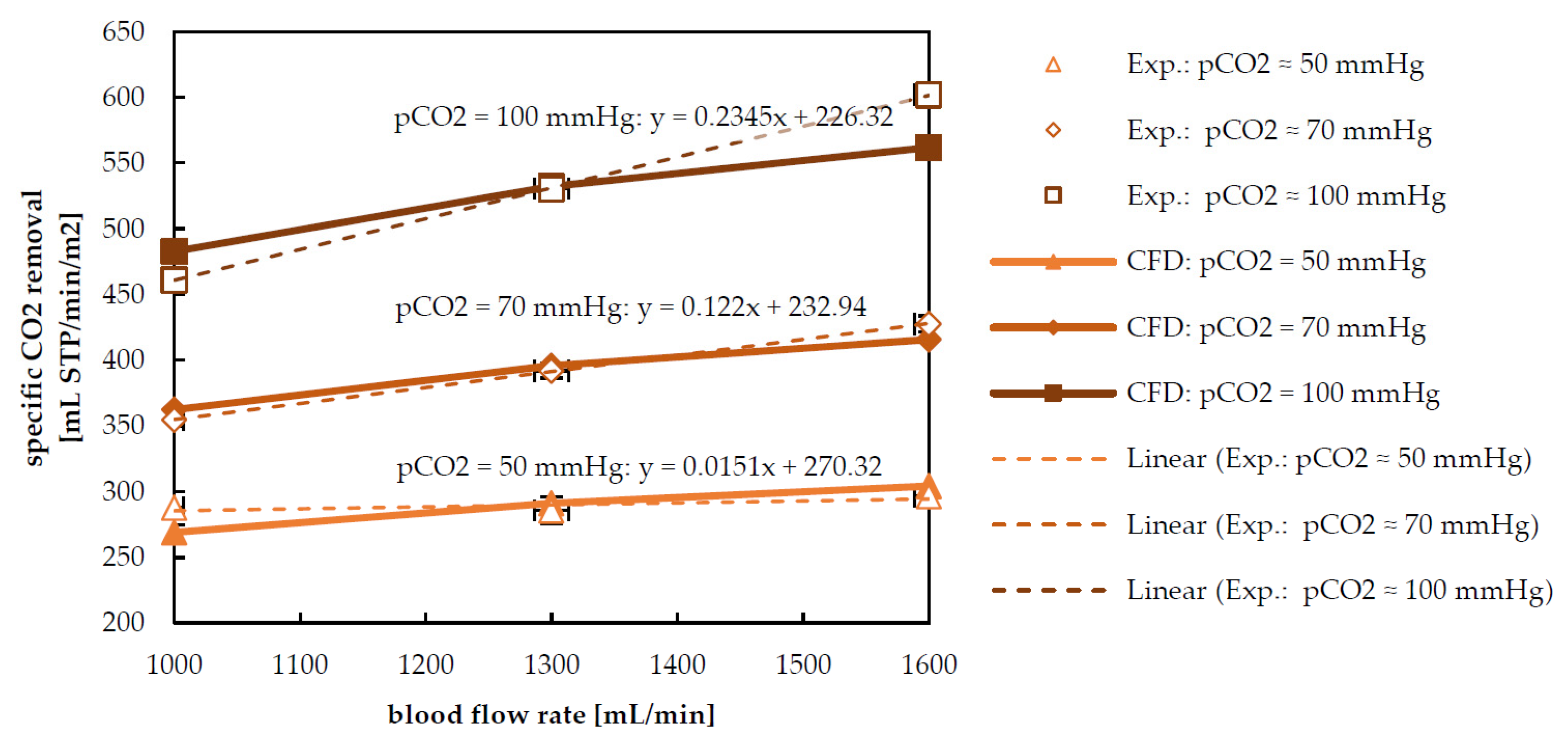
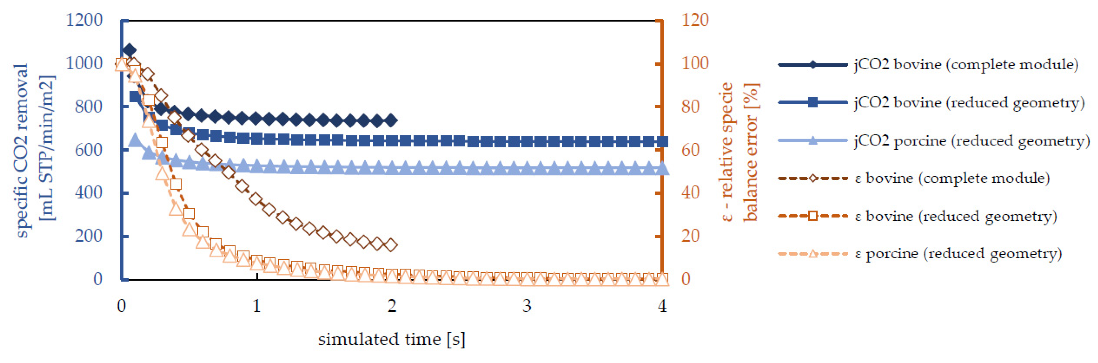
3.2. Species Transport Results
3.3. Computational Costs
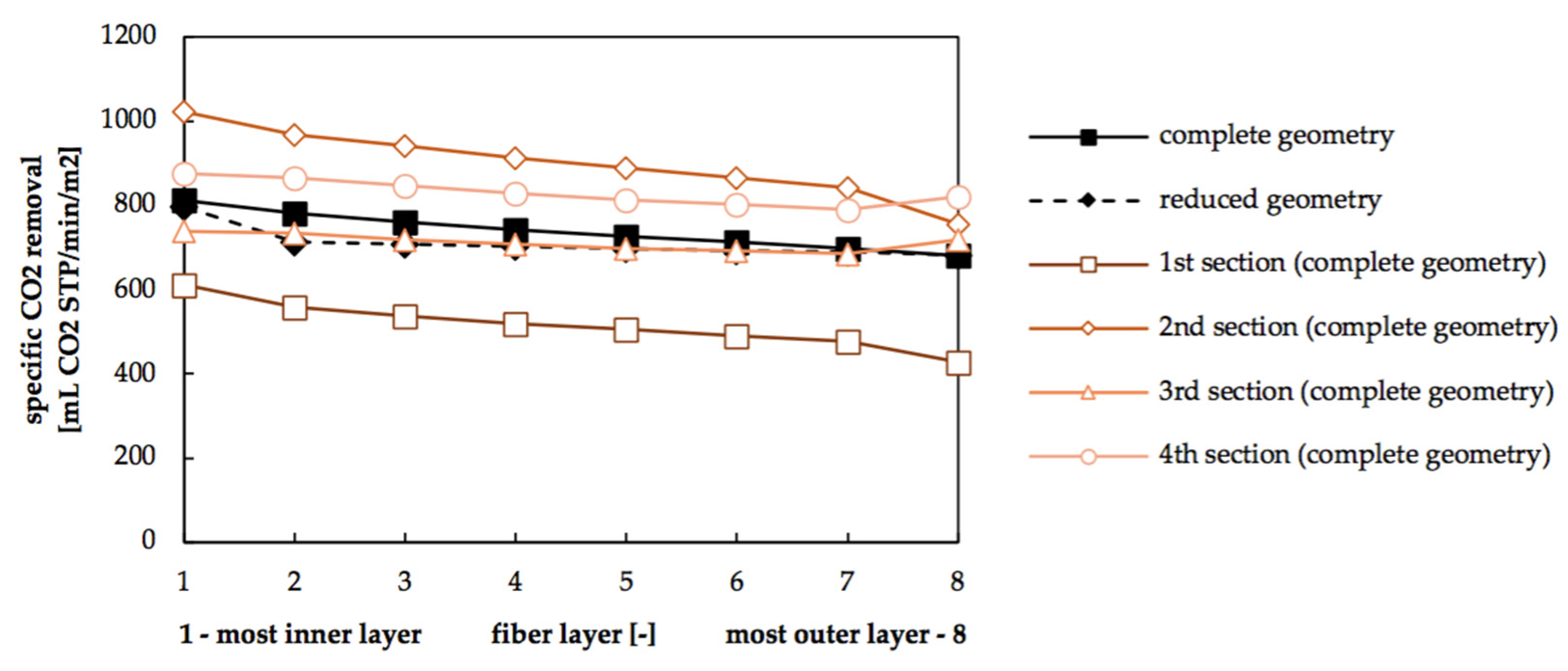
3.4. Radial Dependency of Transmembrane Transport
4. Conclusions
- Flow simulations of a complete module to gain the velocity distribution,
- Identification of velocity components characteristic for transmembrane species transport,
- Development of a simplified hollow fiber packing geometry based on flow simulation results,
- Calculation of matching inlet velocities for the reduced geometry, to account for different flow rates in the complete geometry,
- Species transport simulations of the simplified (reduced) geometry for different flow rates and species compositions,
- Upscaling of the transmembrane transport to the complete geometry.
Author Contributions
Funding
Conflicts of Interest
Nomenclature
| Acronyms | |
| CFD | Computational Fluid Dynamics |
| CO2 | Carbon dioxide |
| HCO3− | Bicarbonate |
| Latin Symbols | |
| A | Membrane area of a computational cell attached to the membrane surface |
| Amembrane,i | Membrane area of reduced (i = reduced) or complete geometry (i = complete) |
| Ainlet | Flow cross-section at inlet |
| Aspacing | Area between two fibers |
| cCO2,total | Total CO2 concentration (dissolved CO2 and bicarbonate) |
| DCO2 | Diffusivity of CO2 in blood |
| DCO2,total | Diffusivity of total CO2 in blood |
| DHCO3- | Diffusivity of HCO3− in blood |
| E(t) | Residence time distribution |
| F(t) | Cumulative distribution function |
| JCO2 | Transmembrane CO2 transport |
| jCO2 | Transmembrane CO2 flux (Transmembrane CO2 Transport per membrane area) |
| L | Characteristic length of Reynolds number |
| n | Total number of fibers |
| ni | Number of fibers in fiber layer (fiber mat winding) i |
| P | Permeance |
| pCO2 | CO2 partial pressure |
| pi | Partial pressure of component i |
| q | Empirical coefficient of CO2 solubility model |
| Re | Reynolds number |
| t | Empirical exponent of CO2 solubility model |
| u | Characteristic velocity of Reynolds number |
| U | Velocity vector field |
| ū | Mean velocity between two fibers |
| uinlet | Uniform inlet velocity |
| umax | Maximum velocity between two fibers |
| uradial | Velocity component in radial direction |
| xj | Unit vector in direction j |
| Greek Symbols | |
| αCO2 | Solubility of CO2 in blood |
| ɣ̇ | Shear rate |
| ΔpCO2 | CO2 partial pressure difference |
| Δpi | Partial pressure difference of component i |
| ε | CO2 species balance error normalized with transmembrane CO2 transport |
| η | Empirical exponent of power law model |
| λ | Slope of CO2 dissociation curve |
| µ | Dynamic viscosity |
| µ0 | Empirical coefficient of power law model |
| µmax | Maximum viscosity of whole blood at low shear rates |
| µmin | Minimum viscosity of whole blood at high shear rates |
| µNewtonian | Newtonian viscosity of whole blood (at high shear rates) |
| ν | Kinematic viscosity |
| τ | Mean residence time |
| ψj | Fraction of velocity component in direction j and velocity magnitude |
References
- Qi, R.; Henson, M.A. Membrane system design for multicomponent gas mixtures via mixed-integer nonlinear programming. Comput. Chem. Eng. 2000, 24, 2719–2737. [Google Scholar] [CrossRef] [Green Version]
- Ghidossi, R.; Veyret, D.; Moulin, P. Computational fluid dynamics applied to membranes: State of the art and opportunities. Chem. Eng. Process. Process. Intensif. 2006, 45, 437–454. [Google Scholar] [CrossRef]
- Low, K.W.Q.; Loon, R.V.; Rolland, S.A.; Sienz, J. Formulation of Generalized Mass Transfer Correlations for Blood Oxygenator Design. J. Biomech. Eng. 2017, 139, 031007. [Google Scholar] [CrossRef] [PubMed]
- Fimbres-Weihs, G.A.; Wiley, D.E. Review of 3D CFD modeling of flow and mass transfer in narrow spacer-filled channels in membrane modules. Chem. Eng. Process. Process. Intensif. 2010, 49, 759–781. [Google Scholar] [CrossRef]
- Dzhonova-Atanasova, D.B.; Tsibranska, I.H.; Paniovska, S.P. CFD Simulation of Cross-Flow Filtration. Ital. Assoc. Chem. Eng. 2018, 70, 2041–2046. [Google Scholar]
- Ghidossi, R.; Daurelle, J.V.; Veyret, D.; Moulin, P. Simplified CFD approach of a hollow fiber ultrafiltration system. Chem. Eng. J. 2006, 123, 117–125. [Google Scholar] [CrossRef]
- Hajilary, N.; Rezakazemi, M. CFD modeling of CO2 capture by water-based nanofluids using hollow fiber membrane contactor. Int. J. Greenh. Gas. Control. 2018, 77, 88–95. [Google Scholar] [CrossRef]
- Miramini, S.A.; Razavi, S.M.R.; Ghadiri, M.; Mahdavi, S.Z.; Moradi, S. CFD simulation of acetone separation from an aqueous solution using supercritical fluid in a hollow-fiber membrane contactor. Chem. Eng. Process. Process. Intensif. 2013, 72, 130–136. [Google Scholar] [CrossRef]
- Zhang, Z.; Yan, Y.; Zhang, L.; Chen, Y.; Ju, S. CFD investigation of CO2 capture by methyldiethanolamine and 2-(1-piperazinyl)-ethylamine in membranes: Part B. Effect of membrane properties. J. Nat. Gas. Sci. Eng. 2014, 19, 311–316. [Google Scholar] [CrossRef]
- Cai, J.J.; Hawboldt, K.; Abdi, M.A. Analysis of the effect of module design on gas absorption in cross flow hollow membrane contactors via computational fluid dynamics (CFD) analysis. J. Membr. Sci. 2016, 520, 415–424. [Google Scholar] [CrossRef]
- Wang, Y.; Brannock, M.; Cox, S.; Leslie, G. CFD simulations of membrane filtration zone in a submerged hollow fibre membrane bioreactor using a porous media approach. J. Membr. Sci. 2010, 363, 57–66. [Google Scholar] [CrossRef]
- Kavousi, F.; Syron, E.; Semmens, M.; Casey, E. Hydrodynamics and gas transfer performance of confined hollow fibre membrane modules with the aid of computational fluid dynamics. J. Membr. Sci. 2016, 513, 117–128. [Google Scholar] [CrossRef] [Green Version]
- He, K.; Zhang, L.-Z. Cross flow and heat transfer of hollow-fiber tube banks with complex distribution patterns and various baffle designs. Int. J. Heat Mass Transf. 2020, 147, 118937. [Google Scholar] [CrossRef]
- Wu, S.-E.; Lin, Y.-C.; Hwang, K.-J.; Cheng, T.-W.; Tung, K.-L. High-efficiency hollow fiber arrangement design to enhance filtration performance by CFD simulation. Chem. Eng. Process.—Process. Intensif. 2018, 125, 87–96. [Google Scholar] [CrossRef]
- Zhuang, L.; Guo, H.; Dai, G.; Xu, Z. Effect of the inlet manifold on the performance of a hollow fiber membrane module-A CFD study. J. Membr. Sci. 2017, 526, 73–93. [Google Scholar] [CrossRef]
- Perepechkin, L.P.; Perepechkina, N.P. Hollow fibres for medical applications. A review. Fibre Chem 1999, 31, 411–420. [Google Scholar] [CrossRef]
- Jaffer, I.H.; Reding, M.T.; Key, N.S.; Weitz, J.I. Hematologic Problems in the Surgical Patient. In Hematology; Elsevier: Amsterdam, The Netherlands, 2018; pp. 2304–2312.e4. ISBN 978-0-323-35762-3. [Google Scholar]
- Federspiel, J.W.; Svitek, G.R. Lung, Artificial: Current Research and Future Directions. Encycl. Biomater. Biomed. Eng. 2008. [Google Scholar]
- Hormes, M.; Borchardt, R.; Mager, I.; Rode, T.S.; Behr, M.; Steinseifer, U. A validated CFD model to predict O₂ and CO₂ transfer within hollow fiber membrane oxygenators. Int. J. Artif. Organs 2011, 34, 317–325. [Google Scholar] [CrossRef]
- Kaesler, A.; Rosen, M.; Schmitz-Rode, T.; Steinseifer, U.; Arens, J. Computational Modeling of Oxygen Transfer in Artificial Lungs. Artif. Organs 2018, 42, 786–799. [Google Scholar] [CrossRef]
- Federspiel, W.J.; Henchir, K.A. Lung, Artificial: Basic Principles and Current Applications. In Encyclopedia of Biomaterials and Biomedical Engineering, 2nd ed.; CRC Press: Boca Raton, FL, USA, 2008; pp. 1661–1672. [Google Scholar]
- Taskin, M.E.; Fraser, K.H.; Zhang, T.; Griffith, B.P.; Wu, Z.J. Micro-scale Modeling of Flow and Oxygen Transfer in Hollow Fiber Membrane Bundle. J. Memb. Sci. 2010, 362, 172–183. [Google Scholar] [CrossRef] [Green Version]
- Harasek, M.; Lukitsch, B.; Ecker, P.; Janeczek, C.; Elenkov, M.; Keck, T.; Haddadi, B.; Jordan, C.; Neudl, S.; Krenn, C.; et al. Fully Resolved Computational (CFD) and Experimental Analysis of Pressure Drop and Blood Gas Transport in a Hollow Fibre Membrane Oxygenator Module. Ital. Assoc. Chem. Eng. 2019, 76, 193–198. [Google Scholar]
- D’Onofrio, C.; van Loon, R.; Rolland, S.; Johnston, R.; North, L.; Brown, S.; Phillips, R.; Sienz, J. Three-dimensional computational model of a blood oxygenator reconstructed from micro-CT scans. Med. Eng. Phys. 2017, 47, 190–197. [Google Scholar] [CrossRef] [PubMed] [Green Version]
- Caretto, L.; Gosman, A.; Patankar, S.; Spalding, D. Two Calculation Procedures for Steady, Three-Dimensional Flows with Recirculation. In Proceedings of the 3rd Conference on Numerical Methods in Fluid Mechanics, Lecture Notes in Physics, 19th ed.; Springer-Verlag: Berlin Heidelberg, Germany, 1973; pp. 60–68. [Google Scholar]
- Johnston, B.M.; Johnston, P.R.; Corney, S.; Kilpatrick, D. Non-Newtonian blood flow in human right coronary arteries: Steady state simulations. J. Biomech. 2004, 37, 709–720. [Google Scholar] [CrossRef] [Green Version]
- Roache, P.J. Perspective: A Method for Uniform Reporting of Grid Refinement Studies. J. Fluids Eng. 1994, 116, 405–413. [Google Scholar] [CrossRef]
- Haddadi, B.; Jordan, C.; Miltner, M.; Harasek, M. Membrane modeling using CFD: Combined evaluation of mass transfer and geometrical influences in 1D and 3D. J. Membr. Sci. 2018, 563, 199–209. [Google Scholar] [CrossRef]
- Svitek, R.G.; Federspiel, W.J. A Mathematical Model to Predict CO2 Removal in Hollow Fiber Membrane Oxygenators. Ann. Biomed. Eng. 2008, 36, 992–1003. [Google Scholar] [CrossRef] [PubMed]
- Windberger, U.; Baskurt, O.K. Comparative hemorheology. In Handbook of Hemorheology and Hemodynamics; IOS Press: Amsterdam, The Netherlands, 2007. [Google Scholar]
- Rauen, H.M. (Ed.) Biochemisches Taschenbuch, 2nd ed.; Springer-Verlag: Berlin Heidelberg, Germany, 1964; ISBN 978-3-642-85768-3. [Google Scholar]


| Notation | Description | Value | Units |
|---|---|---|---|
| αCO2 | Solubility of CO2 in blood | 6.62 E-04 | mL CO2 STP/mL/mmHg |
| DCO2 | Diffusivity of CO2 in blood | 4.62 E-10 | m2/s |
| DHCO3- | Diffusivity of HCO3- in blood | 7.39 E-10 | m2/s |
| λ | Slope of CO2 dissociation curve | 4.25 E-03 | mL CO2 STP/mL/mmHg |
| Blood Flow Rate | Maximum Radial Velocity (umax) | Inlet Velocity (uinlet) |
|---|---|---|
| 1000 mL/min | 0.061 m/s | 0.015 m/s |
| 1300 mL/min | 0.098 m/s | 0.024 m/s |
| 1600 mL/min | 0.126 m/s | 0.031 m/s |
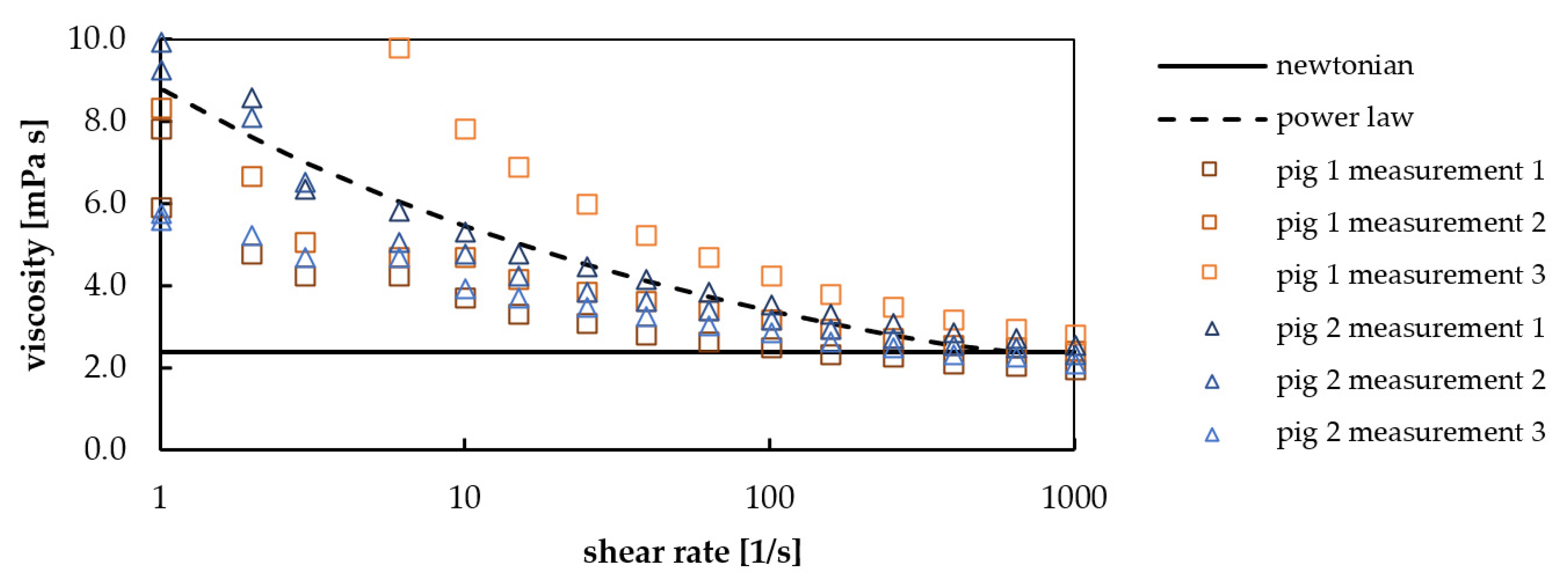
| Blood Type 1 | Shear Rate [1/s] | Dynamic Viscosity [mPa s] | |
|---|---|---|---|
| porcine | 1 | 8.8 (power law model, Figure 6) | |
| porcine | 150 | 3.1 (power law model, Figure 6) | |
| bovine | 1 | 6.7 (mean) [30] | |
| bovine | 150 | 5.8 (mean) [30] |
© 2020 by the authors. Licensee MDPI, Basel, Switzerland. This article is an open access article distributed under the terms and conditions of the Creative Commons Attribution (CC BY) license (http://creativecommons.org/licenses/by/4.0/).
Share and Cite
Lukitsch, B.; Ecker, P.; Elenkov, M.; Janeczek, C.; Haddadi, B.; Jordan, C.; Krenn, C.; Ullrich, R.; Gfoehler, M.; Harasek, M. Computation of Global and Local Mass Transfer in Hollow Fiber Membrane Modules. Sustainability 2020, 12, 2207. https://doi.org/10.3390/su12062207
Lukitsch B, Ecker P, Elenkov M, Janeczek C, Haddadi B, Jordan C, Krenn C, Ullrich R, Gfoehler M, Harasek M. Computation of Global and Local Mass Transfer in Hollow Fiber Membrane Modules. Sustainability. 2020; 12(6):2207. https://doi.org/10.3390/su12062207
Chicago/Turabian StyleLukitsch, Benjamin, Paul Ecker, Martin Elenkov, Christoph Janeczek, Bahram Haddadi, Christian Jordan, Claus Krenn, Roman Ullrich, Margit Gfoehler, and Michael Harasek. 2020. "Computation of Global and Local Mass Transfer in Hollow Fiber Membrane Modules" Sustainability 12, no. 6: 2207. https://doi.org/10.3390/su12062207