Can the Energy Transition Be Smooth? A General Equilibrium Approach to the EROEI


1
CEREC, Université Saint-Louis, 1000 Bruxelles, Belgium
2
IRES, Université Catholique de Louvain, 1348 Louvain-la-Neuve, Belgium
3
LEM-CNRS (UMR9221), Université de Lille, 59655 Villeneuve D’Ascq, France
4
Fonds de la Recherche Scientifique (FNRS), 1000 Bruxelles, Belgium
*
Author to whom correspondence should be addressed.
Sustainability 2020, 12(3), 1176; https://doi.org/10.3390/su12031176
Submission received: 19 December 2019
/
Revised: 16 January 2020
/
Accepted: 24 January 2020
/
Published: 6 February 2020
(This article belongs to the Section Economic and Business Aspects of Sustainability)
Abstract
:The concept of energy return (EROEI ratio) is widely used in energy science to describe the interactions between energy and the economic system but it is largely ignored in macroeconomics. In order to contribute to bridging a gap between these fields of research, we incorporate these metrics into an endogenous growth model with two sectors (energy and final goods) and use this model to analyze the macroeconomic implications of a transition to lower EROEI resources. An approach in terms of net energy allows us (1) to explicitly link the EROEI to macroeconomic variables, (2) to show how it is related to the growth rate of GDP and (3) to obtain a closed-form solution for its long-run value at a general equilibrium level. There is furthermore a tight and decreasing long-run relationship between the EROEI value and the share of investment that must be allocated to the energy sector. Hence, a transition to lower EROEI resources intensifies the rival use of capital in the energy and non-energy sectors and leads to major economic changes, both in the inter-sectoral capital allocation and in the allocation of final output between consumption and investment. We show that a protracted economic contraction may occur before the completion of the transition to renewable energy. We analyze how (1) the magnitude of this contraction and (2) the possibility of an ulterior recovery depend on the initial stock of non-renewables, the potentials of technical progress in the energy and non-energy sectors and the substitutability between capital and energy.
JEL Classification:
Q32; Q43; Q57; O441. Introduction
In a context where world energy demand steadily increases, the primary energy supply to the world economy remains largely dominated by non-renewable energies (NRE): fossil fuels (coal, oil, natural gaz) and incidentally nuclear energy represent more than 85% of the World primary energy supply, renewable energies (RE hereafter) counting for less than 15% (e.g., British Petroleum Energy Outlook [1]). In the future decades, RE production is expected to grow rapidly in absolute terms but according to several organizations (e.g., International Energy Agency [2]), fossil fuels might still represent about three-quarters of the world primary energy mix by 2040. By then, economic growth would therefore remain intensively dependant on NRE. One may, however, question the possibility of maintaining over time such a growth process fed by an intensive use of fossil fuels whose extraction gets increasingly resource consuming. Authors like Meadows et al. [3] (or Turner [4] for an update) and Cappelan-Peréz et al. [5] even doubt that the necessary transition towards RE will allow our rich societies to maintain their level of material welfare.
Energy science highlights why the conditions of energy production matter for economic prosperity. In order to survive or grow, “any being or system” needs energy and “must gain substantially more energy than it uses in obtaining that energy” (Hall et al. [6]). The energy surplus generated by an energy production process can be measured by the ratio of the “Energy Returned On Energy Invested” (EROEI hereafter): it is the ratio of the quantity of energy delivered to the quantity of energy consumed. The energy consumption necessary for energy production can be direct (e.g., coal burned in a boiler) or indirect (e.g., energy necessary for building up the boiler). Energy resources of high quality offer a high EROEI: relatively to their energy density, they require little energy to be discovered, extracted or captured, processed and delivered to the point of use. The EROEI concept can be used at a very micro level to describe the energy return of a particular process (e.g., an oil refinery) but it is also meaningful at a global level to describe the efficiency of the total energy supply to the economy.
The development of contemporary industrial societies over the last two hundred years has relied on an intensive use of fossil fuels offering high EROEI ratios. Such resources have allowed our economies to allocate most of their labor and man-made ressources to other activities than energy production and have thereby contributed to economic expansion and diversification (see a.o. Cleveland [7]). However, a downward trend of the EROEI at a macro level is likely. On the one hand, NRE resources of high quality are progressively depleting and the exploitation of the residual resources is accompanied by a fall in their EROEI (e.g., Hall et al. [8]), either because their energy density is lower and/or because their extraction gets—directly or indirectly—increasingly energy-intensive. On the other hand, most types of RE seem characterized by lower EROEI ratios than conventional NRE (e.g., [8] and Cleveland [9]). Hydropower is an exception but the possibility of developing it further at a global level is limited. If several RE technologies are mature or near-mature (hydroelectricity, wind energy), technical progress in one or another type of RE production (e.g., solar energy) can still improve its efficiency from a purely technological standpoint. However, authors like Moriarty and Honnery [10,11], Dupont et al. [12] (for wind energy) and [13] (for solar energy) argue that the aggregate EROEI of each type of RE will fall as its total production increases, for at least two reasons: (a) the extension of each type of RE production requires investments in progressively less favorable production sites; and (b) “energy ratios for intermittent sources [like wind and solar energy] will fall as energy conversion and storage becomes necessary to balance energy production with demand” [10] (p. 248). On top of that, climate change might negatively affect the technical potential of RE like solar energy and biomass. From a macroeconomic standpoint, if the transition to lower EROEI resources forces the World economy to devote much more inputs to energy supply, it will also exert a drag on economic growth, a.o. because it will exacerbate the rival use of capital in the production of energy and that of final goods. If this rivalry effect was strong enough, investments in the energy sector could crowd investments out of the final goods sector and the transition might then be accompanied by an economic contraction.
Our article explores this possibility in a stylized dynamic general equilibrium model of the World economy. If in energy science, the EROEI metrics is a revelant and widely used concept to describe the interactions between energy production and the economic system (e.g., the review by Rye and Jackson [14]), it has received rather little attention in economic growth literature. We first aim at introducing it into an endogenous growth model in which physical laws limit both the possibility of substituting energy resources by man-made inputs and the potential of energy-saving technological progress. An approach in terms of net energy allows us (1) to link the EROEI metrics to macroeconomic variables, (2) to show how it is related to the growth rate of the economy and (3) to obtain a closed form solution for the long run expression of the EROEI at a general equilibrium level. We then analyze the short and long-run macroeconomic consequences of an energy transition characterized by a decreasing EROEI as a result of the reduction in the NRE stock and a more intensive production of RE. We show (both analytically and numerically) that the transition can be characterized by an economic contraction and highlight what contributes to the occurrence of such contraction and its magnitude.
The article is organized as follows. Section 2 presents a literature review and stresses the original points of our contribution. Section 3 describes the dynamic macroeconomic model and constructs EROEI ratios both at the level of the NRE and RE sub-sectors and at a global level. The model results are presented in Section 4. First, we formally show why a reduction in the EROEI negatively affects economic growth ceteris paribus. We then analyze the stationary state reached once the energy transition is completed and only RE is used. The transitory dynamics are finally studied, mainly on the basis of numerical simulations of a calibrated version of the model. We finally discuss our results.
2. Literature Review
The dynamic macroeconomic model developed hereafter contributes to bridging a gap between economic growth theory and energy science, two fields of research that are used to progress quite independently. Articles interested in the EROEI metrics (e.g., [8,15,16,17]) usually propose partial equilibrium analyses. The GEMBA model developed by Dale et al. [18] and the model proposed by Režný and Burešis [19] are exceptions, but they belong to the system dynamics approach. Contrary to what is usually done in macroeconomic growth theory, they do not explicitly model the economic agents’ behaviors and the formation of market prices. We also refer to [14] for a review of EROEI-dynamics energy-transition models over the last 50 years. In a completely different approach, let us mention [20] where energy transition is analyzed in an agent-based model where agents have bounded rationality and are backward-looking.
While not referring to the EROEI concept, several contributions to economic growth theory deal with energy transition in frameworks where long-term balanced growth remains possible, at least if technological progress can go on endlessly. Let us mention Tahvonen and Salo [21] who propose an optimal growth model that explains the progressive rise and subsequent fall in the use of NRE. However, they do not analyze the determinants of a possible fall in final production or consumption during the transition (albeit some figures of their articles show that such a negative output adjustment may occur in the absence of technical progress). Nor is this issue dealt with in Tsur and Zemel [22], Amigues et al. [23] or in Bonneuil and Boucekkine [24]. Reference [22] characterizes the dynamics of an optimal growth model with R&D investments which reduce the cost of using backstop technologies. Reference [23] analyses the optimal use of a polluting NRE and a clean RE in the presence of a ceiling on the atmospheric carbon concentration. Using viability theory, [24] studies the best transition to a clean RE when an irreversible pollution threshold exists. The possibility of a fall in output and consumption during the energy transition is present in Growiec and Schumacher [25] and Van der Meijden and Smulders [26] but in frameworks without man-made capital (and without extraction costs of NRE in [26]). An output contraction is also a possibility in [27] but in a model where NRE and RE are never used simultaneously.
Two contributions to economic growth theory that explicitly model the EROEI metrics are a discussion paper by Fagnart and Germain [28] (generalized by the present paper) and a subsequent article by Court et al. [29]. However, [29] sticks to a partial equilibrium approach in which the real interest rate is taken as exogenous and the consumers’ behavior (in terms of consumption and saving) is not described. As already mentioned, a declining EROEI intensifies the rival use of capital in the energy and non-energy sectors. The economic consequences of this tension depend on the way aggregate saving reacts, which pleads for a general equilibrium approach in which the agents’ saving behavior is explicitly modeled. Furthermore, [29] supposes that NRE firms have myopic behavior as far as resource extraction is concerned. It also assumes that the production technology of final goods is a Cobb–Douglas relationship combining energy and productive capital even though this assumption, which implies a unitary elasticity of substitution between capital and energy, does not satisfy several physical laws (e.g., Meran [30]). Empirical works also suggest that this elasticity is strictly below 1 (e.g., [31]).
3. Method: A Dynamic General Equilibrium Model of Energy Transition
We study the energy transition in a dynamic general equilibrium macroeconomic model consistent with ecological economics in the line of macroeconomic models like [32,33,34]. More precisely, we assume that (1) the possibility of substituting energy resources by man-made inputs is limited (e.g., [35]) and (2) technological progress is bounded by physical limits (e.g., [30]). In particular, energy efficiency in the final sector is bounded from above, which means that the energy content of final production cannot tend towards zero, even asymptotically.
As we focus on the interactions between the energy and non-energy sectors in a macroeconomic perspective, we adopt an approach in terms of net energy, as already suggested by [36] in a purely accounting macroeconomic framework. We therefore model the part of energy production that is available to the non-energy sector of the economy but do not explicitly model the direct energy consumption by the energy sectors.
For presentation purposes, all abbreviations used for the variables and parameters of the model are listed at the end of the article (see Abbreviations). The price of final goods is normalized to 1 so that all price variables represent real prices.
3.1. The Dynamic System
We consider an economy with two production sectors (final goods and energy), two production factors (capital and energy), and three competitive markets (final goods, capital, and energy). Final goods are used for consumption and investment. The energy sector delivers secondary energy to firms in the final goods sector. It consists of two sub-sectors which respectively produce NRE and RE. Energy supply is initially a mix of NRE and RE. NRE and RE are assumed to be perfect substitutes in the final production process. Energy production requires capital goods delivered by the final goods sector. In each energy sub-sector, the operating cost faced by energy producers increases ceteris paribus when the resource is more intensively used.
There are four types of agents in the model economy: NRE producers, RE producers, producers of final goods and households who consume and save. Appendix A.1–Appendix A.4 describe and solve their decision problems. In this section, we only present the key features of their behaviours and refer the reader to these appendices for further analytical details.
3.1.1. Non-Renewable Energy Sector
Competitive NRE firms run a finite resource stock. Variable denotes the remaining stock at the beginning of period , being the exogenously given initial stock. Variable denotes the resource flow extracted in period t. The resource stock dynamics is therefore given by
Extraction requires equipment goods (capital hereafter). The capital requirements of the NRE sector, , depend on the quantity to extract and on the remaining resource stock : extraction gets more capital intensive ceteris paribus when the resource stock declines. In particular, we assume that is the following function of and :
where is a technological factor which decreases over time as a result of an endogenous technical progress which brings efficiency gains in the extraction process (see Section 3.1.6).
Let be the price of energy in t and be the rental price of capital in t. Let be the discount rate. Appendix A.1 shows that when NRE firms maximize the sum of their discounted profits, the NRE stock is run according to the following Hotelling rule with extraction costs: over the whole period of extraction ,
where if and 0 otherwise. Dynamic Equation (3) means that the optimal extraction path is such that discounted marginal benefits of extraction are equalized across periods, all along the extraction process. Extraction ends in and the optimal value of the discrete variable must be determined by numerical methods.
3.1.2. Renewable Energy Sector
The economy enjoys a constant flow of of RE. We consider a perfectly competitive RE sector. Let be the capital requirement of this sector and its total production level. We assume that the exploitation of flow is impacted by a congestion externality: the RE production cost increases in the exploitation rate of the resource . Consistently with this assumption, Appendix A.2 constructs the following relationship characterizing the aggregate technology of the RE sector:
where and . Technological variable decreases over time as a result of an endogenous technical progress (see Section 3.1.6). The term in on the right-hand side of (4) captures the above mentioned congestion effect. It implies that the capital intensity of RE production increases in the sector production level even if . This property of decreasing returns-to-scale captures, in a stylized way, the various channels through which the energy return of RE production decreases when its production level increases. For instance, operating solar or wind energy requires access to different sites where this energy can be captured. Some sites are less favorable than others and need a higher windmill or more solar panels to obtain the same quantity of energy. In other words, as in a Ricardian resource model, increasing production requires operating less and less favorable sites. We also refer to [10,11,12,13] for other arguments in the case of intermittent RE sources and to [33] for a formal justification of the assumption of decreasing returns-to-scale in the use of a renewable resource in a macroeconomic model. Note that technologies (2) and (4) share a same property: the operating cost of energy production skyrockets when its level reaches the resource limits (i.e., respectively when for NRE and when for RE).
Appendix A.2 shows that the profit maximising behaviour of RE producers leads to the following aggregate relationship between the RE production level and the capital invested in the RE sector :
3.1.3. The Final Goods Sector
Final goods production requires capital and energy. The production technology is of the CES type with constant returns-to-scale: in ,
where is the energy flow and the capital stock allocated to final production; and are productivity factors; is the elasticity of substitution between capital and energy. increases over time as a result of an endogenous technological progress (see Section 3.1.6).
Appendix A.3 shows that the cost-minimising demands for and must verify the following conditions: for all ,
Final production, therefore, gets less energy-intensive and more capital-intensive when the energy price increases relative to the user cost of capital.
Under constant returns-to-scale, perfect competition implies a nil profit: at any output level , . Given (7) and (8), it leads to the following relationship between the price of energy and the rental price of capital:
The term in is the real unit cost of energy and that in is the real unit cost of capital.
3.1.4. Households
The consumer side of the model is quite standard. We consider a representative agent with a very long-time horizon. The household’s preferences are represented by a time-separable iso-elastic utility function. During period t, the household receives all the aggregate income, chooses a consumption level and saves by accumulating capital.
For the sake of analytical tractability, we assume a unitary depreciation rate of capital. In order to achieve a savings level of units of capital at the end of period t, the household must make an investment decision of units of final goods where is the productivity of the transformation of investment goods into productive capital. In , will be rent to firms at price . Hence, saving one unit of income in t (i.e., buying one unit of investment good in t) gives units of capital at the end of t and induces a capital income equal to in . In other words, is the real interest rate in :
As Appendix A.4 shows, the optimal consumption path must verify
where ) is the household’s discount factor and (>0) is the inter-temporal elasticity of substitution in consumption. This equation describes the well-known consumption smoothing behaviour. The inter-temporal consumption path given by (11) implies a corresponding inter-temporal path for savings.
3.1.5. Market Clearing Conditions in Period t
On the final goods market, output is allocated either to consumption or to investment . This market, therefore, clears when
where output supply is given by (6) and the consumption and investment demands follow from the optimal consumption/savings behaviour previously described.
3.1.6. General Equilibrium
The macroeconomic equilibrium in a given period is described by
- the dynamics of the NRE stock (1);
- equations describing the technical progress that governs the evolutions of technological variables , and .
Technological progress is endogenous but bounded by physical laws: the capital intensity of energy production is bounded from below by a strictly positive value (respectively, for RE and for NRE); energy efficiency, , is bounded from above by . This means that it will never be possible to produce a given quantity of final goods with an infinitely small quantity of energy. As we do not aim at modelling R&D activities, we simply formalize technical change as the product of a cumulative learning-by-doing process, which is sector specific: in the final sector, energy efficiency is increasing in the cumulative energy consumption ; the capital intensiveness of each energy sector is decreasing in its cumulative production level. Formally said,
where , and . Asymptotically, tends to ; and respectively tend to and .
Given initial conditions on predetermined variables and values of parameters , the transitory dynamics of the economy consists of two phases: (i) a first phase that lasts periods is characterized by strictly positive RE and NRE productions; (ii) a second phase starts from and is characterized by the absence of any NRE use (). The optimal value of is given by the (implicit) condition detailed in the end of Appendix A.1.
3.1.7. Savings Rate and EROEI Ratios
By definition, the savings rate of the economy, , is given by:
Based on (14), it can be rewritten as
is the fraction of period t output invested in the final goods sector in ; (resp. ) is the fraction of period t output invested in the NRE (resp. RE) sector.
The operationalization of the EROEI definition (i.e., the ratio of the energy delivered by an energy production process to the energy it consumes) raises several questions that are carefully analyzed in [37,38]. These articles define four Energy Return Ratios (ERR), which differ from each other in (a) whether the numerator is defined in terms of gross or net energy and in (b) whether the denominator includes the energy content of all inputs (including the auto-consumption of energy) or only one of the external inputs (excluding the auto-consumption of energy). Since we focus on net energy in our description of the NRE and RE sectors, we compute our EROEI ratios accordingly: the EROEI numerator is defined in terms of net energy, i.e., energy that is available for the non-energy sector of the economy; the EROEI denominator only measures the energy content of the capital goods used in energy production. This way of operationalizing the EROEI concept offers two advantages: it allows us (1) to obtain an explicit expression for the long-run EROEI at the macroeconomic level and (2) to explicitly link the EROEI metrics to macroeconomic variables like the share of capital invested in energy production or the economy growth rate.
In the NRE (resp. RE) sector, (resp. ) units of capital goods are necessary to produce (resp. ) units of net energy, which has required an investment (resp. ); this investment corresponds to a fraction (resp. ) of period output . As units of energy have been necessary to produce , the quantity of energy embedded in the production of (resp. ) is (resp. ). Hence, the EROEI of the NRE and RE sub-sectors (respectively labelled and ) are given by the following ratios:
where the second equality in (18) (resp. (19)) follows from the definition of (resp. ) in (17). The EROEI of an energy sub-sector is the product of the average sectoral productivity of capital ( or ) and two terms that jointly determine the inverse of the energy content of one output unit invested in energy production: a higher means that the energy content of one unit of capital used in t is lower, which contributes to a higher EROEI; a higher productivity of capital in energy production does the same.
3.2. Numerical Simulations
Although the long-run equilibrium of the economy can be analytically described (see next section), solving its transitory dynamics requires to numerically simulate a calibrated version of the model. The calibration is made while assuming that the model describes the World economy. It is detailed in Appendix A.9 and relies on different current values of observed variables at the World level (GDP, energy consumptions, savings rate, etc.) and several reasonable assumptions about the initial NRE stock , the RE flow and the potential of technical progress in the energy and non-energy sectors. With the assumed unitary depreciation rate of capital, we consider a period length of 16 years, which means that a unitary depreciation rate per period corresponds to a linear depreciation rate of a bit more than 6% on an annual basis.
4. Results
4.1. EROEI, Savings and Economic Growth
The first equality in (20) can be rewritten as
This expression gives the set of combinations of and that allow the economy to achieve a given growth rate of energy supply/consumption. It straightforwardly leads to the following proposition:
Proposition 1.
In order to achieve a given growth rate of energy supply, the fraction of final output that must be invested in the energy sector is inversely related to its EROEI.
This illustrates that a declining EROEI intensifies the rivalry between the non-energy and energy sectors about the allocation of savings and investment. A statement similar to that of Proposition 1 can be made for fin al output growth. Indeed, we can write where is the energy content of 1 unit of output in t, i.e., . Therefore,
where the last equality follows from (21). At unchanged energy content of one unit of output (i.e., ), the interpretation of (22) is the same as that of (21) mutatis mutandis: with a lower EROEI, achieving a given rate of economic growth requires raising the share of final output invested in energy production, which means that a lower fraction of final output remains available for consumption and/or investment in the final sector. Obviously, as (22) shows, a decrease in the energy content of final productions (i.e., ) softens the effect of a declining EROEI since it reduces the increase in necessary to achieve a given output growth rate. Expression (22) therefore highlights when energy transition is accompanied by a contraction of output: a deterioration of the EROEI leads to negative output growth if it is not compensated by a sufficiently high increase in the share of investment allocated to the energy sector and/or a sufficiently fast increase in energy efficiency in final production.
4.2. Stationary State Results
When , (15) implies that and are equal to their respective asymptotic values and . The economy then reaches a stationary state. We use letters with asterisk (e.g., , ) to denote the stationary state values of the corresponding variables (e.g., , ).
In the long-run, the energy market clears as ; (11) gives the stationary value of the real rental price of capital and (9) determines the real price of energy:
where the last equality uses (23). Equations (7) and (8) then determine the capital—and energy—intensity of the final output sector (resp. and ) as functions of and . Moreover, , , and are linked by Equations (4) and (5) which hold at any time. The capital market clears as and the good market clearing condition can be written as:
From now on, we assume that energy and capital are complementary factors, i.e., , which is consistent with theoretical works (e.g., [30,35]) and empirical evidence (e.g., [31]).
Lemma 1.
The stationary state equilibrium exists and is unique if households are sufficiently long-term conscious and if investment goods are productive enough, i.e., if β, ζ and φ are large enough:
Proof.
See Appendix A.5. □
Condition (26) is more restrictive when is lower: its right-side is decreasing in , from a value of 1 when (Leontief technology) to a value of 0 when (Cobb-Douglas technology).
Proposition 2.
About the long-run EROEI
- The long run EROEI is given by:
- The share of output allocated to the energy sector is the inverse of the EROEI ratio:
Proof.
See Appendix A.6. □
The following lemma is intuitive and useful to the interpretation of Proposition 2 and the numerical results that will follow.
Lemma 2.
The stationary levels of RE production and final output are increasing in
- the long-termism of private agents β;
- the productivity factors (1) of investment goods φ in capital formation; (2) of energy and capital ζ in final production; (3) of capital in RE production;
- the renewable energy flow ;
- the elasticity of substitution σ between energy and capital in final production.
Proof.
See Appendix A.7. □
Proposition 2 and Lemma 2 suggest the following comments.
- Equation (28) can be easily understood when computing the net energy consumption of the energy sector: it is the energy content of the units of capital invested in RE. Since each unit of final output has an energy content of and is made from of such units, its energy content amounts to . Accordingly, (the ratio between the output of RE sector () and its own energy needs) is equal to , i.e., the inverse of .
- Equation (27), which gives the general equilibrium level of the EROEI, shows that a partial equilibrium reasoning about its determinants may be misleading.First, the EROEI at the global level does not exclusively depend on technological considerations but also on economic factors affecting the savings rate of the economy: in particular, it also depends on the discount factor . Second, changes in technological factors that could improve the EROEI, all other things equal, do not necessarily do so at the global level when they favor economic activity and thereby increase the energy requirements of the economy. Rewriting (28) as shows that only depends on and parameters that influence : at given , a change in a parameter of the model, increases only if it decreases . For instance, a higher (or a higher ) reduces the quantity of final output that must be invested in the RE sector all other things equal, which improves the EROEI of energy production. However, it also induces a rebound effect in the production of energy and finally decreases the EROEI. A larger would save energy at unchanged output level but it has the opposite effect at a general equilibrium level: it ultimately leaves and unchanged.
- The expression of in (27) is larger than 1 because it is the product of two terms (respectively and the expression between square brackets) that are both larger than 1. This result echoes the literature in energy science which argues that a global EROEI sufficiently above 1 is necessary “to maintain what we call civilization” [6], (p. 45).
4.3. Transitory Dynamics Results
4.3.1. A Transition with a Possible Output Contraction
As outlined in Propositions 1 and 2 (point 2), an energy transition with a declining EROEI leads to an important reallocation of capital towards the energy sector. If strong enough, this reallocation could imply a contraction of final output and private consumption. We study hereafter the possibility of such a contraction and the elements that affect its magnitude when it occurs. We also shed light on what influences the ability of the economy to ultimately recover an income level (at least) as high as the peak level reached before the contraction. Our analysis of the model dynamics mainly relies on numerical simulations but two properties regarding the possibility of a contraction of consumption and output can, however, be established formally.
Proposition 3.
- A contraction of private consumption occurs when the real price of an efficient unit of energy (i.e., ) is above its stationary state value, i.e., when
- If a contraction of output occurs, it starts before the completion of the transition, when the increase in RE production is not fast enough to compensate for the decline in NRE production.
Proof.
See Appendix A.8. □
The possibility of an economic contraction during the transition stems from the rival use of capital in the energy and non-energy sectors. Output growth requires more capital and, in spite of (bounded) energy efficiency gains, more energy. Producing more energy requires itself more capital. As long as energy production enjoys a sufficiently high EROEI, energy growth and output growth remain compatible. However, the tension between the two gets stronger if the EROEI declines, which occurs when the two types of energy production get more capital intensive. In order to maintain both energy and output growth in this context, a significant increase in the savings rate becomes necessary. However, if it is not strong enough, the rising capital requirements of the energy sector can crowd investment out of the final goods sector and can put a halt on economic growth, final output starting to contract. This output fall negatively impacts capital accumulation, which deepens the economic contraction.
4.3.2. A Baseline Scenario
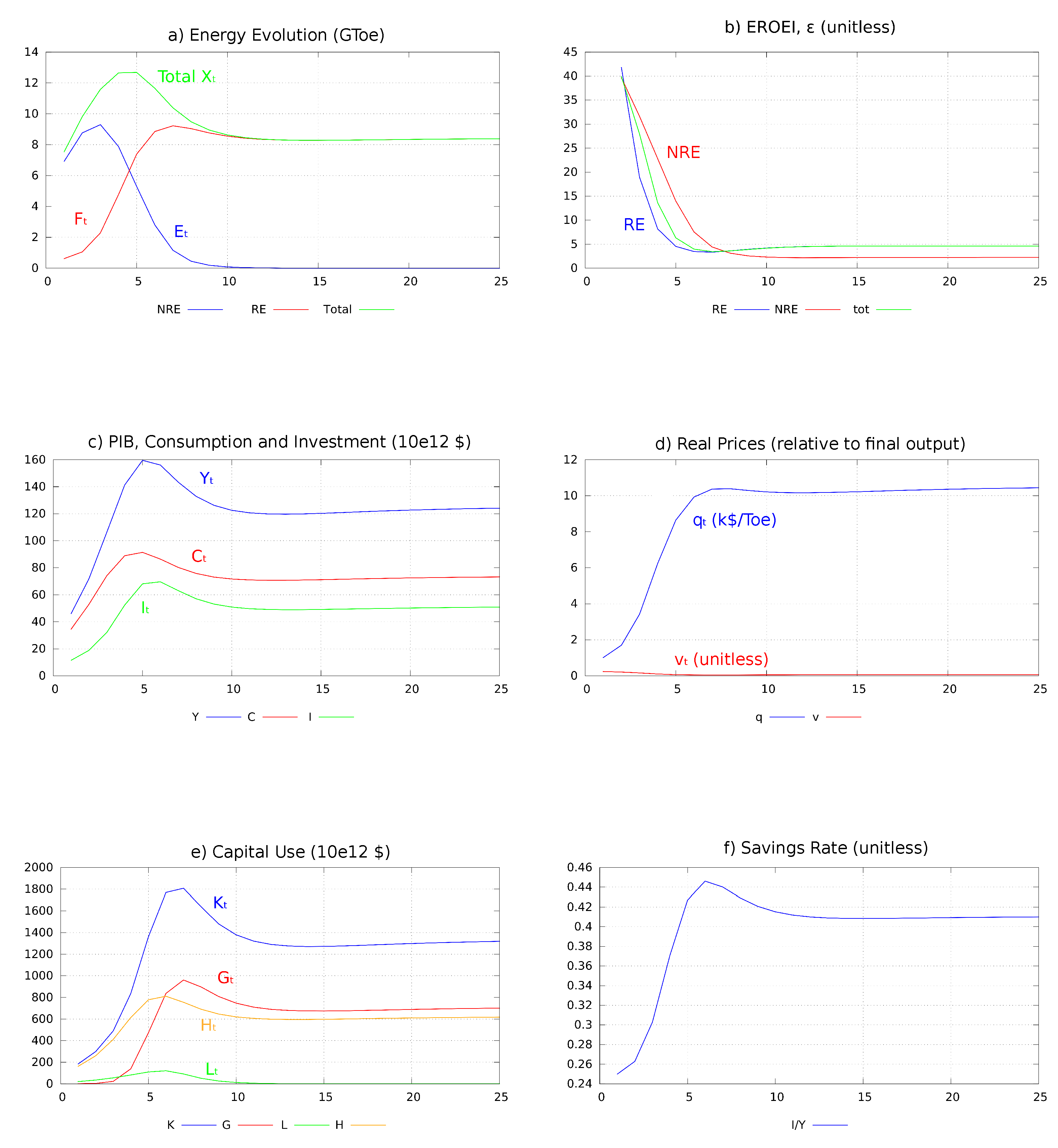
The baseline scenario describes an economy with a rather low initial capital stock () and a potential of energy efficiency gains of 50% () but no technical progress in the energy sectors. As the model is very stylized, the main interest of the numerical analysis is to bring qualitative (not quantitative) insights about the transition dynamics. The general shape of the simulated trajectories of the different variables matters more than their absolute numerical values.
Figure 1a–f hereafter illustrate this scenario. Figure 1a shows the progressive change in the energy mix. NRE production () peaks at the beginning of the trajectory () and then declines monotonically until NRE extraction becomes unprofitable (end of period 12). RE production () also evolves non-monotonically. It first increases and overtakes in period 5. However, it peaks two periods later and then decreases towards its long term value. The figures put forward several striking features of the transition in the baseline scenario.
- The energy transition is characterized by a reduction in the EROEI ratio (Figure 1b) and a progressive rise in the real energy price (Figure 1d). Initially, both NRE and RE production offer relatively high EROEIs (Figure 1b). As hydroelectricity represents the main part of the RE mix in the first period, the initial (calibrated) EROEI of RE is higher than that of NRE. But the two types of energy production become more capital intensive when the NRE stock decreases and RE production rises. The EROEI of each energy production process, therefore, decreases even though energy efficiency gains progressively reduce the energy content of each unit of capital.The fall in the EROEI of RE, however, stops when RE production peaks. After this peak, it slightly improves not only because decreases but also because increases (the energy efficiency gains reduce the energy content of capital used in the RE sector).
- A rapid increase in RE production is only observed when NRE production is still relatively abundant (Figure 1a). This will also be the case in the sensitivity analysis.
- Even though the output level is, in the long run, well above its initial value, it evolves non-monotonically: before the completion of the transition, final output, private consumption and investment (Figure 1c) overshoot the level that the economy is able to sustain in the long run. This contraction of output and consumption starts after the peak in NRE production but well before the end of the NRE extraction (Figure 1a–c). The mechanism that explains this contraction is the one described in the comment following Proposition 3. The contraction stops when the energy transition is completed, output being then 25% lower than at its peak level.
4.4. Sensitivity Analysis
4.4.1. The Impact of the NRE Stock and of Agents’ Short-Termism
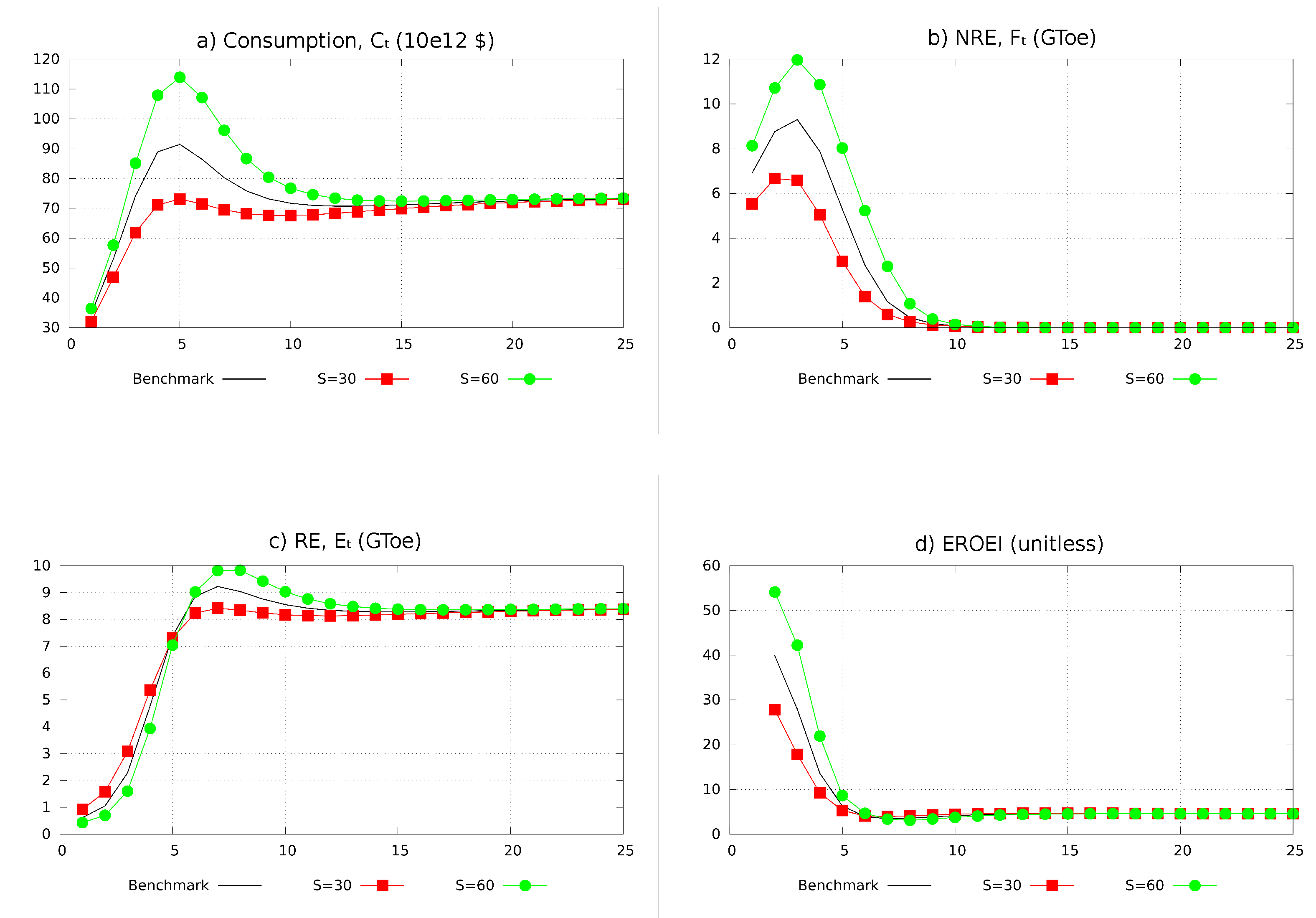
Since the NRE source is no longer extracted in the long run, its initial stock has no impact on the stationary state. It, however, affects the transitory dynamics and has an unambiguously positive impact on the inter-temporal utility level of an infinitely lived representative agent. However, if we interpret the infinitely lived agent as a dynasty of finitely-lived altruist agents (e.g., as in [39]), we can question how the initial abundance of NRE resource affects the material well-being of the generations born during the possible consumption peak and downturn. We can formulate three conjectures that all our numerical simulations confirm.
- The condition of a downward adjustment of consumption and output during the energy transition is more easily met when the initial NRE stock is high. Using point 2 of Proposition 3, we know that with a zero initial stock , an undercapitalized economy (for which ) would not overshoot its stationary levels of consumption and output during the transitory dynamics. This is in accordance with [34] which shows that the transitory dynamics of output in an economy that only uses a constant renewable resource flow is monotonic. By continuity, this certainly remains true if the NRE stock is positive but small enough. Said differently, an overshooting of output and consumption can only occur in an economy with a sufficiently large initial NRE stock. Though it will not be further discussed here, it is also easier to meet the condition of a downward adjustment of consumption and output during the energy transition when economic agents have a lower discount factor β, which leads them to consume the NRE stock faster.
- If a contraction of consumption and output occurs during the energy transition of an economy with an initial NRE stock , its magnitude is increasing in . With a bigger , the NRE production cost and the energy price are initially lower at a given level of final output. Consequently, the overshooting condition (29) will be verified at a higher output level -and possibly at a later time- in a better-endowed economy. Moreover, as the initial NRE stock does not affect the long-run equilibrium, the output contraction will also be larger in an initially better endowed economy.
- A bigger initial stock of NRE resource delays the development of the RE sector. As a bigger initially implies a lower , it also reduces the profitability of the RE sector and initially slows down its development.
Figure 2a–d compare the economy dynamics for three values of : , (baseline scenario) and . All the other model parameters remain unchanged. In the better-endowed economy, the overshooting of consumption and output is amplified as expected (see Figure 2a for ). For the generations born at (or close to) the peak, one can speak of a “malediction of abundance”: with a higher initial NRE stock, they inherit a higher level of consumption but experience a more severe consumption loss later during the transition.
As long as NRE is used, its production is more important in an economy better endowed in NRE, in which it even lasts longer (Figure 2b). The abundance of the NRE stock impacts RE production in two phases: since it initially implies lower energy prices, it first delays investments in the RE sector; but it contributes to a higher EROEI value during a longer time (Figure 2d), which facilitates the production of capital goods and thereby an ulterior development of the RE sector (see Figure 2c). From period 6 and on, RE production becomes larger in the initially better-endowed economy where output growth is stronger.
4.4.2. The Role of the Substitutability Between Capital and Energy
With better substitution possibilities, a given combination of capital and energy allows the economy to produce a higher final output level. The stationary analysis has shown that a higher allows the economy to produce higher long-run levels of output and energy. Since it facilitates final production (and thereby investment), one can expect that a higher σ contributes to a smoother energy transition. This is confirmed by a sensitivity analysis comparing the transitory dynamics of the economy for 4 different values of , , as shown in Figure 3a–d.
A higher leads to a much less conservative extraction of the NRE stock during the first simulation periods (see in Figure 3a). Consequently, NRE production gets more capital intensive and its EROEI is lower (Figure 3b). However, once the economy is better capitalized, a higher enables us to reach a higher production level with less energy. It, therefore, leads to a lower decrease in the EROEI during the transition (Figure 3d) and to a higher long-run EROEI value (if , which is the case for our calibration). With a higher , the magnitude of the output contraction is, therefore, smaller (Figure 3c) and the economy can reach a larger long-run income level. The output contraction even disappears with . However, such a high value of is inconsistent with empirical evidence.
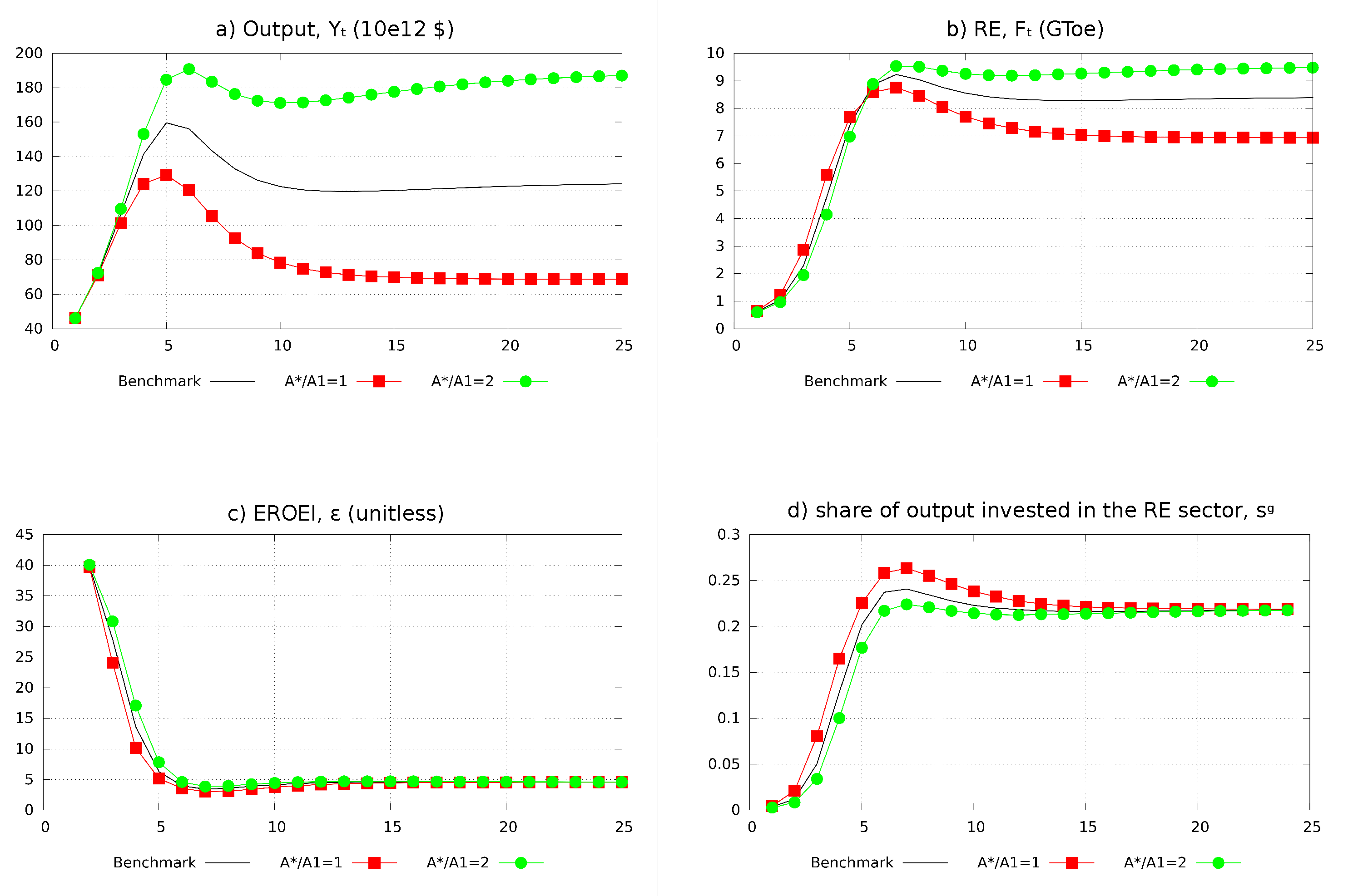
4.4.3. The Role of Technical Progress
Proposition 2 and Lemma 2 have shown that an economy with a larger potential of technical progress (either in the use of energy in the final sector or in the production of energy) can reach a higher long-run output level with a same long-run EROEI. So even if an output contraction occurs during the transition, the potential of technical progress plays a key role in the ability of the economy to recover long-run output levels at least equal to the peak levels reached before the end of the NRE production. On this basis and given Equation (22) following Proposition 1, one can safely infer that a larger potential of technical progress (either in the use of energy or in its production) facilitates the transition.
Figure 4a–d compare the trajectories of output, RE production, global EROEI and for three values of : , (benchmark value) and (no technical progress). Given the law of motion of (see (15)), a higher implies stronger energy efficiency gains during the whole trajectory of . Hence, when is higher, (1) output growth is initially stronger and output peaks at a higher level; (2) the consecutive output contraction is relatively weaker; (3) the economic recovery is stronger after the completion of the transition.
As long as NRE remains relatively abundant, the development of RE (Figure 4b) is somewhat delayed when energy efficiency gains are stronger. However, later in time, stronger efficiency gains, which transitorily improve the EROEI of the RE sector, are favorable to RE production. Consequently, the economy can produce additional units of final output and energy while investing less in RE production (see in Figure 4d). This induces a positive feedback loop between the production of capital goods and that of energy.
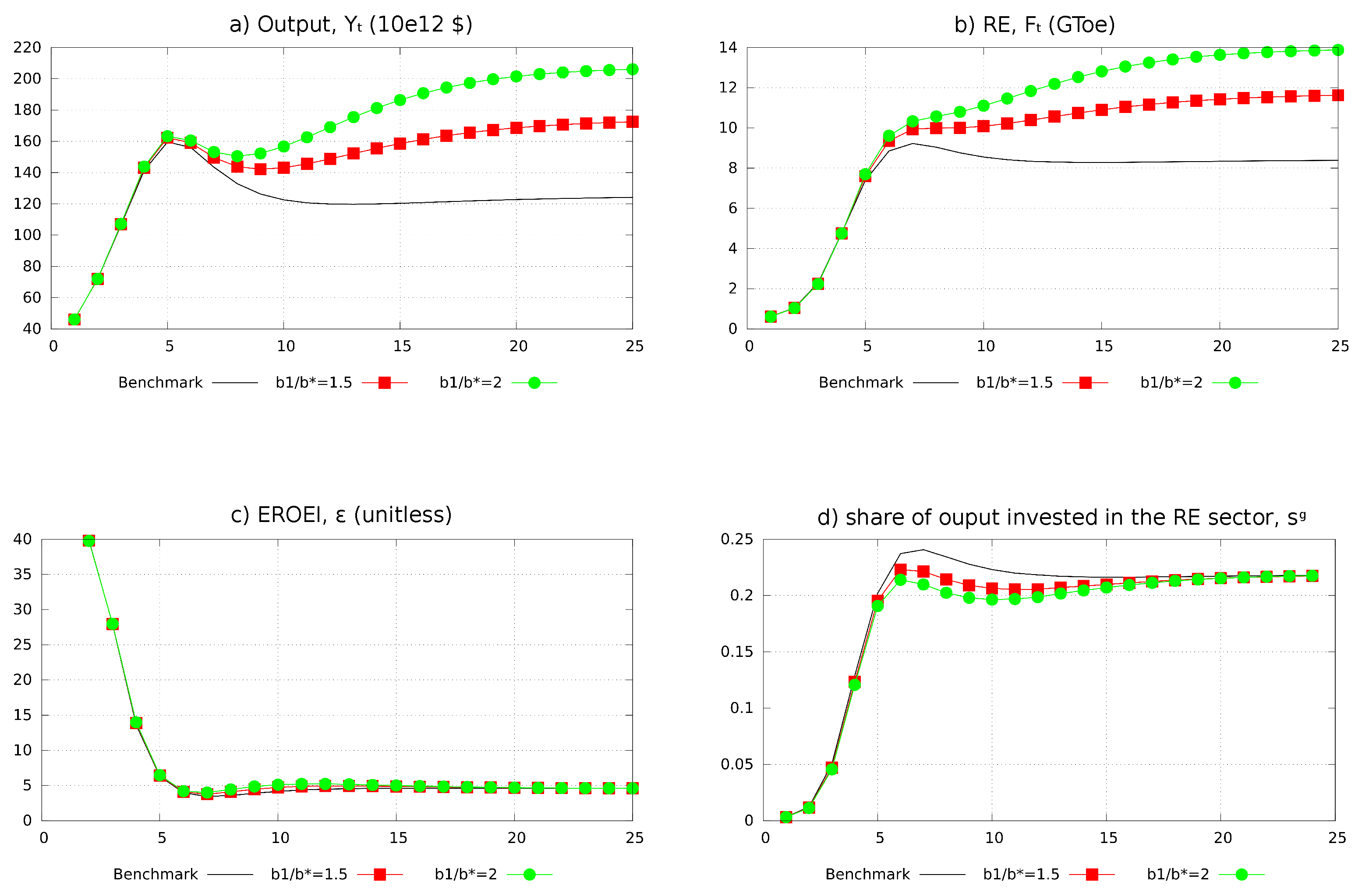
Figure 5a–d illustrate the impact of technological progress in the RE sector and compare the trajectories of final output, RE production, global EROEI and for three values of the ratio : (baseline scenario), and . With a lower , the economy converge towards higher levels of output and RE production (Figure 5a,b). However, because RE production is relatively small in the first periods and the productivity gains in the RE sector stem from a learning by doing process, the difference between the baseline and the other scenarios is initially very weak. It only becomes larger after the output peak (and therefore later than in the sensitivity analysis on ). Stronger productivity gains in the RE sector unsurprisingly facilitate the transition by allowing the economy to produce more RE while investing less in the RE sector (Figure 5d). The EROEI evolution is very similar in the three simulations: stronger productivity gains improve the EROEI ceteris paribus but this effect is counterbalanced by the impact of a larger RE production on the capital intensity of the energy sector.
5. Discussion and Conclusions
In the following discussion, we first compare our results to those of contributions to economic growth theory (EGT hereafter) and to energy science, in particular to the Dynamic Systems Approach to Energy Transition (DSAET hereafter). We then suggest several policy implications that can be drawn from our analysis. We finally mention a few limits of our work which open the way to future research.
Contributions to EGT can be into two categories. A first one (hereafter labeled neoclassical models of energy transition) assumes that the productivity of energy (ratio in our notations) can grow limitless. Under this assumption, the economy can converge to a balanced growth path after the completion of the transition (e.g., [21,26]). Our contribution and [29] belong to a second-category which acknowledges that the productivity of energy is bounded by physical laws. Consistently with ecological economics, our dynamic general equilibrium approach supposes that these laws limit both the possibility of substituting energy resources by man-made inputs and the potential of energy-saving technological progress. In such a framework, the economic consequences of the energy transition are more severe than in neoclassical models. More precisely, in an economy characterized by laissez-faire (or free markets), the energy transition may have negative consequences on global economic activity (GDP) and private consumption: after a phase of growth, these variables may enter into a phase of protracted contraction before converging to a stationary state. Such a possibility is absent from most neoclassical contributions to EGT. In neoclassical models where it is nevertheless present (e.g., [26]), it is usually not more than a temporary break in balanced growth.
With respect to the partial equilibrium model of [29] and recent contributions to DSAET [19], the first original contribution of our article is to allow us to explicitly link the EROEI metrics to macroeconomic variables and to obtain analytical results regarding the determinants of the EROEI value and its economic implications (a.o. on the GDP growth rate). These results, which do not depend on a particular model calibration, are useful complements to the purely numerical results of the DSAET. Furthermore, they show that at a global (general equilibrium) level, the value of the EROEI is not determined by purely technological and physical considerations but also by economic factors that influence the intensity of energy demand/production.
The transitory dynamics of GDP in our model are qualitatively similar to that obtained in [19,29] but our contribution explores more extensively what contributes to an economic contraction and to its magnitude. The transition to lower EROEI resources is characterized by important changes both in the inter-sectoral capital allocation and in the allocation of final output between consumption and investment (savings). In our baseline scenario, for instance, the savings rate rises from 25% to more than 40%, in accordance with the Business as Usual scenario explored in [19]. A lower EROEI constrains the economy to allocate more capital to energy production and the resulting tensions between the use of capital in the energy and non-energy sectors exert a drag on economic growth: a more capital intensive energy production slows down investments in the final goods sector ceteris paribus and thereby, the production of future capital goods used in energy and non-energy sectors. The rise in the savings rate and technological progress contribute to reducing these tensions. However, as the EROEI further decreases, they may not be sufficient to prevent a crowding out of investment from the final goods sector. In such a case, the transition is accompanied by a contraction of economic activity and private consumption. We formally show that such a contraction (if it occurs) starts before the completion of the transition, when the increase in RE production is not fast enough to compensate the decline in NRE production. The magnitude of this contraction is larger when (i) the initial stock of NRE is higher, (ii) the potentials of technical progress in the energy and non-energy sectors are lower and (iii) the substitutability between capital and energy in final production is weaker. It is also larger when agents are more short-term minded (i.e., have a higher discount factor).
Our numerical simulations also highlight the interaction between the abundance of NRE resources and the development of the RE sector. A greater abundance of NRE first lowers the price of energy, which discourages the investments in RE. However, it increases the EROEI and allows for more growth, which facilitates the development of RE. The net effect is a priori ambiguous but simulations show that the first effect dominates at first and the second one dominates later in the transition.
Let us also outline that under laissez-faire and except under very special conditions, the economic path followed during the energy transition is not sustainable from an intergenerational equity point of view since the welfare of successive generations evolves non-monotonically. As emphasised by Pearce, “Sustainability (…) implies something about maintaining the level of human well-being so that it might improve but at least never declines (…)” ([40], p. 48). Promoting sustainability, therefore, suggests to act—when possible—on variables or parameters that influence the magnitude of the economic downturn observed during the transition. Our results point in the direction of a more conservative exploitation of NRE resources. A smaller initial NRE stock indeed implies smaller peaks in output and consumption ceteris paribus and so leads to a smoother transition towards the stationary state. This suggests that a policy of conservation of NRE resources (which implies to voluntary refrain from exploiting a part of the NRE stock) would favor a more sustainable energy transition. It would allow for a faster development of the RE sector, which would furthermore contribute to the fight against climate change.
Literally implementing this conservation policy whose economic consequences can be unequally spread across countries may require international agreements that can be hard to (if not out of) reach. However, this type of policy can be (at least partly) mimicked by using appropriate fiscal instruments. This echoes the proposition (made in [29]) to tax NRE while simultaneously subsidizing investments in the RE sector. Alternatively (or complementarily), a conservation policy could also be approached by encouraging economic agents to be more long-term conscious in their decision making, in particular in the NRE sector: discounting future profits with a lower discount rate leads to more conservative exploitation of the NRE stock and to a smoother transition.
Our model could be generalized in various directions. First, it assumes a perfect substitutability between non-renewable and renewable energies. This is certainly a very optimistic assumption and one can suspect that imperfect substitutability could worsen the economic implications of the transition. Secondly, the model could be enriched to take into account issues linked to pollution and climate change which make energy transition more necessary, but possibly less easy. Thirdly, the population could be endogenized. This would allow us to assess the impact of the transition on per capita income and to study feedback loops between demography and energy transition. Lastly, the design of more precise policy recommendations pleads for a more disaggregated version of the model: a more disaggregated description of the energy and non-energy sectors or a multi-country perspective would certainly be interesting in this respect.
Author Contributions
J.-F.F., M.G. and B.P. were involved in all stages of the work, from conceptualization to writing. All authors have read and agreed to the published version of the manuscript.
Funding
This research received no external funding.
Acknowledgments
We would like to thank three anonymous referees for their comments. We also thank David de la Croix and Louis Possoz for comments on an earlier version of this article.
Conflicts of Interest
The authors declare no conflict of interest.
Abbreviations
List of the endogenous variables at the aggregate level
| Energy production and NRE stock | |
| NRE production during period t | |
| RE production during t | |
| total energy production during t | |
| NRE stock at the beginning of period t | |
| last period of NRE extraction | |
| global EROEI of the energy sector in t | |
| Capital stock | |
| Aggregate capital stock at the beginning of period t | |
| Capital stock used in the final goods sector in t | |
| Capital stock used in the RE sector in t | |
| Capital stock used in the NRE sector in t Final production and its allocation | |
| Final output level in period t | |
| Private consumption in period t | |
| savings rate in t | |
| fraction of period t output invested in the final production sector | |
| fraction of period t output invested in the RE sector | |
| fraction of period t output invested in the NRE sector | |
| Technological variables | |
| Factor of energy efficiency in the final goods sector t | |
| Factor of capital intensiveness of the RE production process in t | |
| Factor of capital intensiveness of the NRE extraction process in t | |
| Real prices | |
| real price of energy in t | |
| real interest rate in period t | |
| real rental price of capital in t | |
| firms’ discount factor of period t profits | |
| List of parameters | |
| Inter-temporal elasticity of substitution of consumption | |
| Households’ subjective discount factor | |
| Capital elasticity of RE production at the firm level | |
| Productivity factor of the investment goods in the capital formation | |
| Elasticity of substitution between energy and capital in the final goods technology | |
| Capital productivity factor in the final goods technology | |
| a | Weight of energy in the final goods technology |
| RE flow per period | |
| Initial NRE stock | |
Appendix A.
Appendix A.1. NRE Sector
The optimization problem of the representative NRE producer is depicted as follows:
subject to constraints (1) and (2), with given.
We focus on the contemporary energy transition and therefore on trajectories characterized by a first phase where both NRE and RE are used and followed by a second phase where NRE extraction has ceased. The solution to (A1) is therefore such that
- or for where () is the optimal time length during which the NRE stock is exploited;
- or for .
We solve this problem in two steps. In a first step, taking as given, we determine the optimality conditions for the other decision variables conditionally on this value of . Using (1) and (2), this problem can be reduced to:
under the constraints . We can write the Lagrangian of this problem as:
where the ’s are multipliers and is given. The first order optimal conditions are:
We look for a solution where and where is the final period of extraction and In other terms:
We describe the solution starting from the last period.
In , (A6) and (see (A7)) imply that Then, using (A4) in , we obtain Since (see (A7)), it also means that Next using (A4) in , we obtain Since (see (A7)), we can equivalently write Repeating the same reasoning until we obtain:
In (A4) ⇒. Using (A8) and , this expression can be rewritten as
Using the definition of we then obtain (3).
Let be the vectors that are solutions to (A1) at given . These vectors depend on .
In a second step, we then determine the optimal value of , which is the solution to:
Because is discrete, it can only be determined by numerical methods.
Appendix A.2. RE Sector
Let be the energy supply of a RE producer and its capital requirement. RE production is described by the following technological relationship
is a productivity term. In period ), and are chosen by solving
After substituting by (A12) into (A13), we rewrite the problem of a firm as: . The first-order optimality condition is , or , which leads to
At the RE sector level, the total energy supply and capital demand are given by and .
Appendix A.3. Final Goods Sector
With the price of final goods normalized to 1, the cost minimization problem of a final firm can be written as subject to constraint (6).
The expressions of the marginal productivity of and write respectively as
The expressions of first-order conditions (7) and (8) follow straightforwardly. The Euler theorem for homogeneous function of degree 1 next implies:
where (A15) makes use of the equality between the marginal product of each factor and its price. After substituting and by their expressions in (7) and (8), we can rewrite (A15) as (9).
Appendix A.4. Consumers’ Behaviour
In a given period t, the representative household’s income consists of capital rent and profits . Her budget contraint of period t can be written as
where is the investment level in period t.
The household’s preferences are represented by a time-separable iso-elastic utility function with a discount factor . The inter-temporal decision problem writes as:
subject to constraint (A16) and with and given. T is the exogenous time horizon (possibly infinite). The first-order conditions for an interior solution lead to (11). The optimal consumption/savings behaviour must also satisfy the terminal condition .
Appendix A.5. Proof of Lemma 1
A stationary state equilibrium must be such that . Using (24), this implies (26) when (what we assume). As , (26) also requires that is sufficiently larger than the right-hand-side of the inequality.
Given and (uniquely determined by (23) and (24)), Equations (8) to (5) give , and . Given , (4) is an equation in which admits a unique solution. With , the right-hand-side of (4) is monotonically increasing in from 0 (when ) up to infinity (when ). For a value of the left-hand-side given by (5), there is therefore a unique that verifies (4). , , , and can next be obtained.
Appendix A.6. Proof of Proposition 2
Appendix A.7. Proof of Lemma 2
Given (23), is decreasing in or but does not depend on any other parameter. Given (24), the larger or , the larger . Hence a larger or implies larger values of (cfr. (8) and (cfr. (5) but a lower (cfr. (7). Via (4), a higher implies a higher . An increase in combined with a decrease in implies a more than proportional increase in .
A higher imply a proportional increase in (cfr. (24)). This implies an increase in , thereby in (via (5)) and so in (via (4)) and . As and so do not depend on (see (27) and (28)), increases in the same proportion as .
A higher increases (cfr. (24)) but leaves unchanged. This implies 1) an increase in (via (5)) and so in (via (4)) and in , 2) a decrease in (via (7)), which means that increases more than .
The positive impact of and on both and is obvious: Equations (23) to (5) do not depend on these two parameters, which do not affect , and the ratios , and . At unchanged , (4) implies a positive effect of both and on and thereby on (via (8)).
In order to analyze the impact of a change in , it is useful to define the real unit cost of energy : . In a stationary state, it is linked to by the following relationship which follows from (9)
The differential of (A18) in the case of a change in leads to
This derivative is positive if the logarithmic term is negative i.e., if (using (23))
If this inequality is not verified, is decreasing in . However, is necessarily increasing in : in the case of a change in , the differential of the first equality of (24) writes as
After dividing this equality by and using (A19), one obtains
When , the expression multiplying dd is positive. In order to show that the right-side of (A20) is necessarily positive, let us first note that
where the first line of equalities uses the definition of in (24) and the second line uses the link between the price of capital and its real unit cost (which is equal to ).
Using the last two expressions, the right-side of (A20) can be rewritten as follows
Let us show that reaches a minimum value of 0 in and is strictly positive for any other value of .
The FOC for a minimum of () gives . is convex since is
For , , therefore, reaches a minimum of . It is strictly positive otherwise. Hence, and (via (5)) increase in . Given (4), so is .
Other parameters being given, (28) and the second equality in (27) imply that a change in affects (and thereby ) in the same way as . If , and are decreasing in . An increase in (which increases as we have seen) therefore implies an increase in more than proportional to the one in . If , and are increasing in . increases as well but to a lesser extent than .
Appendix A.8. Proof of Proposition 3
- Point (1) implies that if a contraction in consumption starts in a period t, we then have (since there is no contraction in ) and therefore . Since , these inequalities imply thatHence, the contraction in starts at a time where RE production and its capital requirements increase. Moreover, inequality and (7) jointly imply thatSince , a fall in output () will therefore occur only if total energy production decreases: in such a case, one hasThe combination of (A22) and (A23) proves ad absurdio that if a contraction occurs, it starts when NRE is still used. Assume indeed that the decrease in consumption and output starts when NRE resource is not extracted anymore (so that and ): (A22) would then imply that , i.e., , which contradicts (A23).
Appendix A.9. Calibration
Given that a period lasts 16 years, periods , , … correspond respectively to the intervals 198–1996, 1997–2012, … In the following (as well as in the simulations), the value of a variable for a given period is its average annual value over the period.
According to [2], world secondary energy consumption in 2012 is billions of tons of oil equivalent (GToe hereafter) and total primary energy supply is GToe. Moreover the average annual secondary energy consumption in period 1, , is approximately 7.8 GToe. On the basis of annual world GDP values, we compute = 46 $ (In dollars of 2005). We also obtain values for and in the same way.
Considering the value of 4.3 from [41] as an upper bound for the world capital ratio, we estimate the initial ratio between global production (GDP) and capital () to be 4.0. This ratio and give an initial capital stock equal to $.
According to [1], the share of renewable energy (with hydroelectricity) in the world’s primary energy mix is around % in 2014 and the annual average in period 1 is around %. Assuming that the share of renewable resources in secondary energy is close to their share in primary energy, we use this last data to fix the ratio . Then we obtain (GToe) and (GToe). Assuming the initial non-renewable stock to be equivalent to a hundred times the current annual secondary energy consumption (which is very uncertain), we have (GToe).
In EU27, USA, Japan, China and Russia, the manufacturing sector (an energy-intensive sector) is characterized by a real unit energy cost () much larger than 10% ([1]). Thus 10% can be considered as a lower bound for the aggregate real unit energy cost and we set . Then we are able to compute the initial price of energy .
The investment (in percent of GDP) varies between 22.2% and 25% during the interval 1997–2012 according to [2]. The average savings rate over period 1 (resp. 0) is (resp. ). We so obtain a value of given by:
In order to calibrate the initial EROEIs of NRE and RE, we use Equations (18) and (19). We divide RE production into two parts: hydroelectricity, denoted by superscript “hy” hereafter, and the other renewable sources (wind, solar, geothermal, …), denoted by superscript “re”. The aggregate EROEI for RE can be written as follows
Assuming that , we can rewrite the last equality as follows:
Based on ranges given in [42], we take the following EROEI values: 30 for wind energy, 10 for solar energy, 25 for geothermal energy. Taking the average of these values, the EROEI for RE without hydroelectricity is 21.67. For hydroelectricity, we assume a EROEI equal to 80 (a plausible guess) and a share of hydroelectricity in total RE production initially close to 86.9% (see [1]). Equation (A25) then gives:
The approach is the same for NRE. We assume the following EROEIs: oil: 30, coal: 70, gas: 30, nuclear: 6. Given the shares of each source in period 1 given by [1] (oil: 38.5%, coal: 30.6%, gas: 24.7% and nuclear: 6%), we obtain:
Using the definition of , we can then determine the value of : so that .
Then we obtain . In the same way, we estimate by . Finally, we find . Using this value, we estimate : .
As far as the elasticity of substitution between energy and capital is concerned, we are not aware of any paper estimating at a World level using a CES production function. However, several papers have estimated nested CES functions at the industry and/or country level. They indicate that the possibility of substitution between energy and a mix of capital and labour is rather weak. Reference [43] obtains an elasticity of substitution of for the West-German Industry. Using industry- level data from 12 OECD countries, [31] obtains industry estimates ranging from 0.17 to 0.65 and country estimates ranging from 0.17 to 0.61. He also tests the hypothesis of a unitary elasticity (the Cobb-Douglas case) and rejects it for all the countries and industries of his data set. Reference [44] also concludes that capital and energy are complementary factors in the manufacturing industry of seven OECD countries. Based on these estimates, we set to .
Technical progress in the final and RE sector is described by the following functional forms:
where and are initial conditions the calibration of which is detailed below and and are strictly positive parameters.
On the basis of [45], we estimate to 1/45 the ratio between current exergy obtained from RE (geothermal, tidal power, solar, water power, ocean waves, biomass, etc.) and the potential exergy that could be obtained from these resources. Assuming that , we obtain (GToe). Given , we determine and : and .
Given , , , , , and considering Equations (7)–(9) in , we obtain a system of three equations with three unknowns: a, and . We solve the system by a simple all-in-one algorithm and we obtain: , and .
Given values of , , , , and , optimality condition (11) imposes a constraint on the choice of and . Fixing , we obtain , which corresponds to a time preference rate of 2.6% on an annual basis.
References
- British Petroleum. BP Statistical Review of World Energy 2018. Available online: bp.com/statisticalreview (accessed on 10 January 2020).
- International Energy Agency. World Energy Outlook 2019; IEA: Paris, France; Available online: www.iea.org/reports/world-energy-outlook-2019 (accessed on 10 January 2020).
- Meadows, D.; Randers, J.; Meadows, D. Limits to Growth. The 30-Year Update; Chelsea Green Publishing Company: White River Junction, VT, USA, 2004. [Google Scholar]
- Turner, G. Is Global Collapse Imminent? An Updated Comparison of The Limits to Growh with Historical Data; Research Paper n0 4; Melbourne Sustainable Society Institute: Parkville, Australia, 2014. [Google Scholar]
- Capellán-Pérez, I.; Mediavilla, M.; de Castro, C.; Carpintero, Ó.; Miguel, L.J. Fossil fuel depletion and socio-economic scenarios: An integrated approach. Energy 2014, 77, 641–666. [Google Scholar] [CrossRef]
- Hall, C.; Balogh, S.; Murphy, D. What is the minimum EROI that a sustainable society must have? Energies 2009, 2, 25–47. [Google Scholar] [CrossRef]
- Cleveland, C. Energy Return on Investment EROI, Encyclopedia of the Earth. 2008. Available online: http://eoarth.org/article/Energy_return_on_invesment (accessed on 30 June 2016).
- Hall, C.; Lambert, J.; Balogh, S. EROI of different fuels and the implications for society. Energy Policy 2014, 64, 141–152. [Google Scholar] [CrossRef] [Green Version]
- Cleveland, C. (Ed.) Encyclopedia of Energy; Elsevier: Dordrecht, The Nertherlands, 2004. [Google Scholar]
- Moriarty, P.; Honnery, D. What is the global potential for renewable energy? Renew. Sustain. Energy Rev. 2012, 16, 244–252. [Google Scholar] [CrossRef]
- Moriarty, P.; Honnery, D. Can renewable energy power the future? Energy Policy 2016, 93, 3–7. [Google Scholar] [CrossRef]
- Dupont, E.; Koppelaar, R.; Jeanmart, H. Global available wind energy with physical and energy return on investment constraints. Appl. Energy 2018, 209, 322–338. [Google Scholar] [CrossRef]
- Dupont, E.; Koppelaar, R.; Jeanmart, H. Global available solar energy under physical and energy return on investment constraints. Appl. Energy 2020, 257, 113968. [Google Scholar] [CrossRef]
- Rye, C.; Jackson, T. A review of EROEI-dynamics energy-transition models. Energy Policy 2018, 122, 260–272. [Google Scholar] [CrossRef]
- King, C.; Hall, C. Relating financial and energy return on investment. Sustainability 2011, 3, 1810–1832. [Google Scholar] [CrossRef] [Green Version]
- Murphy, D.; Hall, C. EROI or energy return on (energy) invested. Ann. N. Y. Acad. Sci. 2010, 1185, 102–118. [Google Scholar] [CrossRef]
- Heun, M.; de Wit, M. Energy return on (energy) invested (EROI), oil prices, and energy transitions. Energy Policy 2012, 40, 147–158. [Google Scholar] [CrossRef]
- Dale, M.; Krumdieck, S.; Bodger, P. Global energy modelling? A biophysical approach (GEMBA) Part 1: An overview of biophysical economics. Ecol. Econ. 2012, 73, 152–157. [Google Scholar] [CrossRef]
- Režný, L.; Bureš, V. Energy transition scenarios and their economic impacts in the extended neoclassical model of economic growth. Sustainability 2019, 11, 3644. [Google Scholar] [CrossRef] [Green Version]
- Ponta, L.; Raberto, M.; Teglio, A.; Cincotti, S. An Agent-based Stock-flow Consistent Model of the Sustainable Transition in the Energy Sector. Ecol. Econ. 2018, 145, 274–300. [Google Scholar] [CrossRef] [Green Version]
- Tahvonen, O.; Salo, S. Economic growth and transitions between renewable and nonrenewable energy resources. Eur. Econ. Rev. 2001, 45, 1379–1398. [Google Scholar] [CrossRef]
- Tsur, Y.; Zemel, A. Scarcity, growth and R&D. J. Environ. Econ. Manag. 2005, 49, 484–499. [Google Scholar]
- Amigues, J.-P.; Moreaux, M.; Schubert, K. Optimal use of a polluting non-renewable resource generating both manageable and catastrophic damages. Ann. Econ. Stat. 2011, 103/104, 107–130. [Google Scholar] [CrossRef] [Green Version]
- Bonneuil, N.; Boucekkine, R. Optimal transition to renewable energy with threshold of irreversible pollution. Eur. J. Operat. Res. 2016, 248, 257–262. [Google Scholar] [CrossRef] [Green Version]
- Growiec, J.; Schumacher, I. On technical change in the elasticities of resource inputs. Resour. Policy 2008, 33, 210–221. [Google Scholar] [CrossRef] [Green Version]
- Van der Meijden, G.; Smulders, S. Technological change during the energy transition. Macroecon. Dyn. 2018, 22, 805–836. [Google Scholar] [CrossRef] [Green Version]
- Jouvet, P.-A.; Schumacher, I. Learning-by-doing and the costs of a backstop for energy transition and sustainability. Ecol. Econ. 2011, 73, 122–132. [Google Scholar] [CrossRef] [Green Version]
- Fagnart, J.-F.; Germain, M. Can the Energy Transition Be Smooth? CEREC Working Paper 2014/11; Université Saint-Louis: Bruxelles, Belgium, 2014. [Google Scholar]
- Court, V.; Jouvet, P.-A.; Lantz, F. Long-Term Endogenous Economic Growth and Energy Transitions. Energy J. 2018, 39, 29–57. [Google Scholar] [CrossRef]
- Meran, G. Thermodynamic constraints and the use of energy-dependent CES-production functions A cautionary comment. Energy Econ. 2019, 81, 63–69. [Google Scholar] [CrossRef]
- Van der Werf, E. Production functions for climate policy modeling: An empirical analysis. Energy Econ. 2008, 30, 2964–2979. [Google Scholar] [CrossRef] [Green Version]
- Krysiak, F. Entropy, limits to growth, and the prospects for weak sustainability. Ecol. Econ. 2006, 58, 182–191. [Google Scholar] [CrossRef]
- Fagnart, J.-F.; Germain, M. Quantitative versus qualitative growth with recyclable resource. Ecol. Econ. 2011, 70, 929–941. [Google Scholar] [CrossRef]
- Germain, M. Equilibres et effondrement dans le cadre d’un cycle naturel. Brussels Econ. Rev. Cahiers Econ. Bruxelles 2012, 55, 427–455. [Google Scholar]
- Anderson, C.L. The production process: Inputs and wastes. J. Environ. Econ. Manag. 1987, 14, 1–12. [Google Scholar] [CrossRef]
- Fagnart, J.-F.; Germain, M. Net energy ratio, EROEI and the macroeconomy. Struct. Chang. Econ. Dynam. 2016, 37, 121–126. [Google Scholar] [CrossRef]
- Brandt, A.R.; Dale, M. A general mathematical framework for calculating systems-scale efficiency of energy extraction and conversion: Energy Return on Investment (EROI) and other energy return ratios. Energies 2011, 4, 1211–1245. [Google Scholar] [CrossRef] [Green Version]
- Brandt, A.R.; Dale, M.; Barnhart, C. Calculating systems-scale energy efficiency and net energy returns: A bottom-up matrix-based approach. Energy 2013, 62, 235–247. [Google Scholar] [CrossRef]
- Michel, P.H.; Thibault, E.; Vidal, J.-P. Intergenerational Altruism and Neoclassical Growth Models. In Handbook of the Economics of Giving, Altruism and Reciprocity: Applications Vol. 2; Kolm, S.-C., Mercier Ythier, J., Eds.; North-Holland: Amsterdam, The Netherlands, 2006; pp. 1055–1106. [Google Scholar]
- Pearce, D.W. Economic Values and the Natural World; Earthscan: London, UK, 1993. [Google Scholar]
- Piketty, T. Le Capital au XXIe Siècle; Seuil: Paris, France, 2013. [Google Scholar]
- Gupta, K.; Ajay, K.; Hall, C. A review of the past and current state of EROI data. Sustainability 2011, 3, 1796–1809. [Google Scholar] [CrossRef] [Green Version]
- Kemfert, C. Estimated substitution elasticities of a nested CES production function approach for Germany. Energy Econ. 1998, 20, 249–264. [Google Scholar] [CrossRef]
- Forito, G.; van den Bergh, J.M. Capital-energy substitution in manufacturing for seven OECD countries: Learning about potential effects of climate policy and peak oil. Energy Effic. 2016, 9, 49–65. [Google Scholar] [CrossRef]
- Valero, A.; Martinez, A. Inventory of the exergy resources on earth including its mineral capital. Energy 2010, 35, 989–995. [Google Scholar] [CrossRef]
Figure 1.
Energy transition in the baseline scenario. The horizontal axis of each figure gives the simulation time period. The vertical axis gives the value of the displayed variable(s). Dollar values are expressed in trillions () of 2005 dollars.
Figure 1.
Energy transition in the baseline scenario. The horizontal axis of each figure gives the simulation time period. The vertical axis gives the value of the displayed variable(s). Dollar values are expressed in trillions () of 2005 dollars.

Figure 2.
The impact of the non-renewable energies (NRE) stock. The horizontal axis of each figure gives the simulation time period. Final consumption (a) is expressed in trillions of 2005 dollars. Energy production (b,c) is expressed in GToe.
Figure 2.
The impact of the non-renewable energies (NRE) stock. The horizontal axis of each figure gives the simulation time period. Final consumption (a) is expressed in trillions of 2005 dollars. Energy production (b,c) is expressed in GToe.

Figure 3.
The role of the substitutability between capital and energy. The horizontal axis of each figure gives the simulation time period. Energy production (a,d) is expressed in GToe. Output (c) is expressed in trillions of 2005 dollars.
Figure 3.
The role of the substitutability between capital and energy. The horizontal axis of each figure gives the simulation time period. Energy production (a,d) is expressed in GToe. Output (c) is expressed in trillions of 2005 dollars.

Figure 4.
The role of the potential of energy efficiency gains in the final sector. The horizontal axis of each figure gives the simulation time period. Output (a) is expressed in trillions of 2005 dollars. Energy production (b) is expressed in GToe.
Figure 4.
The role of the potential of energy efficiency gains in the final sector. The horizontal axis of each figure gives the simulation time period. Output (a) is expressed in trillions of 2005 dollars. Energy production (b) is expressed in GToe.

Figure 5.
The role of technical progress in the RE sector. The horizontal axis of each figure gives the simulation time period. Output (a) is expressed in trillions of 2005 dollars. Energy production (b) is expressed in GToe.
Figure 5.
The role of technical progress in the RE sector. The horizontal axis of each figure gives the simulation time period. Output (a) is expressed in trillions of 2005 dollars. Energy production (b) is expressed in GToe.

© 2020 by the authors. Licensee MDPI, Basel, Switzerland. This article is an open access article distributed under the terms and conditions of the Creative Commons Attribution (CC BY) license (http://creativecommons.org/licenses/by/4.0/).
Share and Cite
MDPI and ACS Style
Fagnart, J.-F.; Germain, M.; Peeters, B. Can the Energy Transition Be Smooth? A General Equilibrium Approach to the EROEI. Sustainability 2020, 12, 1176. https://doi.org/10.3390/su12031176
AMA Style
Fagnart J-F, Germain M, Peeters B. Can the Energy Transition Be Smooth? A General Equilibrium Approach to the EROEI. Sustainability. 2020; 12(3):1176. https://doi.org/10.3390/su12031176
Chicago/Turabian StyleFagnart, Jean-François, Marc Germain, and Benjamin Peeters. 2020. "Can the Energy Transition Be Smooth? A General Equilibrium Approach to the EROEI" Sustainability 12, no. 3: 1176. https://doi.org/10.3390/su12031176
Note that from the first issue of 2016, this journal uses article numbers instead of page numbers. See further details here.