Channel Structure Strategies of Supply Chains with Varying Green Cost and Governmental Interventions

Abstract

Environmental concerns make enterprises pay more attention to green manufacturing. The emerging green supply chain inevitably will compete with the traditional supply chain. In order to evaluate the competitiveness of supply chains and the impact on channel structure strategy, we develop four game models for two competing supply chains according to their channel structure strategies. Green marginal manufacturing cost, demand sensitivity of green level, and governmental interventions are considered. We study how retail prices, green levels, and profits are influenced by channel structure choice and governmental interventions. Analytical results indicate that the substitutability of products affects channel structure strategy. When the substitutability of products is relatively low, centralization–centralization is the unique Nash equilibrium. However, when the substitutability of products is relatively high, both centralization–centralization and decentralization–decentralization are the Nash equilibriums. Centralization–centralization is a prisoner dilemma, while decentralization–decentralization can make the green supply chain achieve optimal profit. Then, the green marginal manufacturing cost and demand sensitivities of the green level play important but different roles in channel structure strategy of the competing supply chains. Further, whether Nash equilibriums are the optimal strategy depends on governmental intervention. Relatively severe governmental intervention might realize a relatively higher green level, but may not always achieve the lowest retail price for the green supply chain. However, a relatively moderate governmental intervention might achieve a relatively lower green level.

1. Introduction

With the increasing concerns on environmental issues, many enterprises have undergone greening in practice, e.g., GE, Lenovo, and Linglong Tire. Scholars have also conducted extensive research on green (sustainable) supply chain management, such as the vehicle supply chain (Peterson and Michalek [1]), the food supply chain (Nakandala and Lau [2]), and the shipping supply chain (De et al. [3] and De et al. [4]). In the circumstances where the green supply chain (GSC) and the traditional supply chain (TSC) coexist, there is inevitable competition between them for the substitutability of products. The competition between supply chains affects the pricing and green level decisions of channel members and further influences the channel structure strategy of supply chains. The most common vertical channel structures are centralization and decentralization [5]. A centralized structure means channel members act as a whole, while in a decentralized structure, channel members act independently. Clearly, for two competing supply chains, one supply chain’s channel structure will affect the other supply chain’s channel structure choice. Therefore, a more thorough understanding of how the competition between GSC and TSC affects their channel structure strategies and their profitability is necessary and interesting, which is the content of our research.

Because green products require higher manufacturing and investment costs than traditional ones, GSC often has disadvantages in competition with TSC when providing substitute products. In order to encourage the development of GSC, governments may enact incentive regulations or policies in favor of green supply chains. Governments usually subsidize GSCs and penalize TSCs. For example, the American Recovery and Reinvestment Act of 2009 provides a tax credit of USD 2500 per plug-in hybrid electric vehicle sold (a minimum of 4 kWh battery capacity) and an additional USD 417 for each additional kWh of battery capacity above 4 kWh [6]. The Chinese government levies taxes on enterprises whose products are not up to environmental standards (Ministy of Ecoology and Environment of the People’s Republic of China. Available online: http://www.mee.gov.cn/). Governmental interventions have important effects on the competition of these supply chains, which further affects a supply chain’s channel structure strategy. One of the main objectives of this paper is to investigate the impact of governmental interventions on channel structure strategy and the equilibrium solutions of the supply chains, and further study what interventions can realize the optimal equilibrium and promote the development of GSC efficiently.

For green products, the first and most important step is the design stage. So, when a manufacturer produces or sells its products, the design step is often finished. For that reason, some studies treat the green level as an exogenous parameter. More generally, enterprises may take the design, production, and sale cycle of green products as a whole process. That is when they design their green products, they have already considered the production and sale stages. This motivates us to research the effect of the endogenous green level on the channel structure strategies of competing supply chains. Moreover, raw materials play a vital role in the production and consumption of green products. Generally, the higher the green level, the higher the quality of raw materials. In other words, the higher the green level, the higher the unit production cost and the retail price. Green marginal manufacturing cost (GMMC) increases the competition between supply chains, and further affects the channel structure strategy. Therefore, it is of great significance to study the effect of the cost structure of green products on channel structure strategy.

In addition, environmental awareness changes consumer’s purchasing behavior. There are some convincing evidences that consumers are more willing to buy environmentally friendly products than before [7]. For example, as carried out by European Commission in 2008, 75% of Europeans are ready to buy green products even if they cost a little more, up from 31% in 2005 [8]. That is, consumers have different demand sensitivities to green and traditional products. Generally speaking, the increase of consumers’ demand for green products is greater than the decrease in the demand for traditional products for each additional green level of products. Therefore, the other focus of this paper is to investigate the influence of the consumer’s environmental awareness and purchasing behavior on channel structure strategy of supply chains.

Specifically, this paper investigates the channel structure strategy of two competing supply chains (GSC and TSC) under governmental interventions. Considering the GMMC and green consumers’ demand sensitivity to green level (DSGL), GSC and TSC choose their own channel structures: a centralized or decentralized structure. We try to answer the following research questions: Given the competitor is centralized, what structure is better for GSC or TSC? Vice versa, what channel structure is better if the competitor is decentralized? Further, which channel structure is the Nash Equilibrium? How do the key variables (such as GMMC, the endogenicity of the green level, and governmental intervention) affect the channel structure? Moreover, which channel structure is beneficial for the environment or consumers? To answer these questions, we established four game models to analyze the competition between GSC and TSC under four combinations of channel structures, respectively. We find that both centralization–centralization (CC) and decentralization–decentralization (DD) are possibly the Nash equilibriums, which depend on the channel competition between supply chains when the green level is exogenous. However, when the green level is endogenous, numerical results show that governmental interventions (green level floor and adjustment factor) play important but different roles in channel structure strategy for both GSC and TSC. Further, the CC scenario may not realize the optimal profits for the two supply chains, while the DD scenario might make the GSC achieve the maximum profit. In addition, relatively stringent governmental intervention is necessary for the development of GSC.

2. Literature Review

This work is closely related to green supply chain management (GSCM), channel competition, channel structure strategy, and governmental intervention for supply chains.

2.1. Green Supply Chain Management

The literature of GSCM focuses on how supply chains make their strategies to not only increase competitiveness to further capture additional market share, but also protect the environment. Studies about GSCM mainly focus on two aspects: product recycling or reverse logistics, and making green products with a low environmental cost. This study is related to the latter aspect. Many researchers have conducted relevant studies on green products. For instance, Tseng et al. [9] evaluate green innovation practices focusing on managerial, process, product, and technology innovation. Biswas and Roy [10] study the impact of consumer behavior on the emerging economy by exploratory study with the green product. Fang et al. [11] refine influencing factors of the formation and evolution of collaborative innovation networks and the evolution indicators of green innovations performance. Seman et al. [12] examine the mediating effect of green innovation on the relationship between GSCM and environmental performance. Yu et al. [13] investigate the relationships between supply chain quality integration, GSCM, and environmental performance and establish a structural equation model using the data collected from 308 manufacturing companies in China. Chen et al. [14] study the reverse logistics pricing strategy of a GSC from the view of customers’ environmental awareness. Different from the above literature that treats green levels as an input parameter, some studies treat it as a decision variable. For example, from the consumer’s perspective, Zhang et al. [6] investigate the impact of consumer environmental awareness (CEA) on order quantities and channel coordination. Ghosh and Shah [15] explore cooperation issues and examine the impact of cost-sharing contracts on the key decisions of GSC players. Chen et al. [16] investigate joint decisions on production and pricing for green crowdfunding products of different quality levels. By introducing competing products, Zhang et al. [17] consider the coordination strategy of a green supply chain with hybrid production mode. Jian et al. [18] study a multi-objective optimization model of GSC by considering environmental benefits. Motivated by the studies, we treat green level as an exogenous parameter at first to investigate the impact of the competitiveness on the channel structure strategy of supply chains. Then, we treat it as an endogenous variable to study the effect of green level and the cost structure on the channel structure strategies of supply chains. Considering green level in the context of channel structure strategy is another contribution of this paper.

2.2. Channel Competition

Channel competition has become more evident because competition in markets is now shifting from the competition between enterprises to the competition between channels [19]. Since McGuire and Staelin [20] first considered a price competition between two suppliers and explored the effect of product substitutability on optimal retailer distribution, channel competition has become an interesting topic. For instance, Wu et al. [21] studied bargaining in competing supply chains with demand uncertainty. Majumder and Srinivasan [22] studied the competition and leadership of network supply chains. Chakraborty et al. [23] investigated the cost-sharing mechanism for product quality improvement in a supply chain under competition. Wang and Liu [24] studied vertical contract selection under chain-to-chain service competition in a shipping supply chain. The above literature studies the competition between TSCs. As green products occupy more shares in the market, the competition of GSCs with multiple products attracts increasing attention. For example, Zhang et al. [7] developed a multi-product newsvendor model for a supply chain manufacturing green and non-green products under competitive and cooperative situations. By considering competitive scenario, Yalabik and Fairchild [25] examined the effects of consumer, regulatory, and competitive pressure on firm investments in environmentally-friendly production. Compared with the existing literature focusing on the multi-product supply chain, this paper emphasizes the channel structure strategy with multi-chains under governmental intervention. Nobari et al. [26] studied a chain-to-chain competition between two supply chains using a multi-objective mathematical model. Li and Li [27] studied the game model and the equilibrium structures of two reverse supply chains under competition in product sustainability. Unlike Nobari et al. [26] and Li and Li [27], we mainly focus on the impacts of the substitutability of products and governmental interventions on the channel structure strategy of competing GSC and TSC. Further, we consider different prices of competing products, which is also different from Li and Li [27].

2.3. Channel Structure Strategy

Since Spengler first considered the channel structure of supply chains in 1950 [28], researchers have studied this topic extensively. Generally, there are two channel structures vertically in a supply chain: centralization and decentralization. From the traditional viewpoint, because of the double marginalization effect, a centralized strategy is more conducive to supply chains than a decentralized strategy. For example, Spengler [28] believes that concentration could improve the performance of a supply chain. With the deepening of the research, scholars have considered various factors and believe that a decentralized supply chain can achieve or even exceed the performance of a centralized supply chain. For example, Su and Zhang [29] believe that a decentralized supply chain under a wholesale price contract has a higher performance than a centralized supply chain under the consideration of strategic consumers. Liu and Tyagi [30] studied the impact of upstream supply chain channel decentralization on the supply chain when competitive enterprises can outsource production to their upstream suppliers. Results show that when the production is endogenous, downstream enterprises can still benefit from the decentralized channels of the upstream. Zhao and Shi [31] studied the channel structure strategy of supply chains under competition with multiple suppliers and a single retailer. Results show that decentralization is better when competition is fierce. However, centralization is better when there are multiple vendors. Some studies have considered the environmental impact of supply chains when discussing supply chain channel strategy. Xia et al. [32] examined service level and distribution channel decisions for competing supply chains with a focus on how service competition affects the channel structure. Xing et al. [33] investigated the channel structure of a GSC in the context of competition. Results showed that when the potential market size of traditional products is small or substitutability of products is high, decentralization is better for traditional manufacturers; otherwise, traditional manufacturers will choose a centralized strategy. However, green manufacturers will always choose a centralized strategy. The research of Bian et al. [34] showed that, unlike the traditional double marginalization effect, a monopolistic manufacturer benefits from the decentralization when the environment is sufficiently polluted by its manufacturing technology. In some cases, decentralized manufacturers can benefit from tax reductions. Inspired by the debates on channel structures, this study investigates the channel structure strategy of two competing supply chains (GSC and TSC), considering the green product cost structure and governmental two-way interventions. This study differs from Xing et al. [33] and Bian et al. [34]. Xing et al. [33] emphasized the effect of market size and substitutability of products but did not consider a green product manufacturing cost increase with its green level and governmental intervention. However, Bian et al. [34] studied the distribution channel strategies of monopolistic manufacturers and emphasized an environmental tax but no subsidy.

2.4. Governmental Intervention

Governmental intervention has been widely considered in GSC in recent years. However, the impact of governmental intervention on supply chain competition appears to be controversial. Some researchers insist that government intervention can be beneficial for the development of the GSC. For example, Sheu and Chen [35] analyzed the effects of governmental intervention on GSC competition by using a three-stage game model. Numerical results revealed that social welfare and chain-based profits can be improved by 27.8% and 306.6%, respectively, compared with the case without intervention. Atasu and Wassenhove [36] studied the implications of environmental legislation on the collection and recycling of used electrical and electronics products. Ghazanfari et al. [37] studied the impact of government incentives on the fresh-product supply chain. Results show that government incentives can increase the profit of all members. However, others hold the opposite view; they think governmental intervention may be detrimental to the competition between supply chains. For example, Sheu [38] investigated the negotiations between producers and reverse-logistics suppliers for cooperative agreements under government intervention. Results indicated that government intervention may result in adverse effects on profits and social welfare. Besides, Droste et al. [39] investigated institutional conditions facilitating the transition towards a green economy of government intervention. Madani and Rasti-Barzoki [40] considered the role of government and interactions between the government and supply chain members’ decisions. Li et al. [41] investigated the issues of the recycling and remanufacturing of the construction of a closed-loop supply chain; results showed that governmental regulations could effectively increase the recycling amount. Liu and Nishi [42] stated that government intervention could influence the market demands and return rates. Ma et al. [43] studied the method to drive green innovation, and the results show that the government should subsidize both the retailer and the manufacturer to improve the green innovation level. Yang and Xiao [44] studied the role of governmental intervention in GSC under different channel power scenarios. Dixit et al. [45] investigated government-supported health-care supply chain enablers in rural areas of India to minimize wastage of generic medicines. Government subsidies are conducive to promoting green innovation in enterprises. Choi and Luo [46] studied government sponsor schemes and environment taxation waiving schemes on data quality of a sustainable fashion supply chain. Guo et al. [47] reported that high levels of government subsidies can weaken the relationship of financial slack and R&D investment but strengthen the relationship of R&D investment and firm performance. From the above controversial arguments, it is necessary to investigate how government intervention affects green levels and retail prices of competing supply chains under different channel structures. Furthermore, what role will governmental intervention play in the competition and the equilibrium results?

By investigating the roles of the substitutability of products and consumer demand sensitivity to green levels (DSGL) in competing supply chains under different channel structure strategies, and examining the impact of governmental intervention and green marginal manufacturing cost (GMMC) on the development of GSC, this work bridges between behavioral decision theory and GSCM. Unlike the extant literature, we model the impact of government intervention on channel structure strategy and study how channel structure strategy depends on the intervention, GMMC, and consumers’ DSGL. Our findings show that substitutability of products affects the channel structure strategy of both GSC and TSC. Government intervention, GMMC, and consumers’ DSGL play important but different roles in channel structure strategies and pricing and green level decisions of the competing supply chains.

The rest of this paper is organized as follows. Section 3 briefly introduces the problem formulation and notations. Section 4 analyzes the equilibrium strategies under different channel structure scenarios with an exogenous green level. Section 5 analyses the equilibrium strategies under different channel structure scenarios with endogenous green levels and provides numerical examples. Section 6 summarizes the results and indicates future research directions.

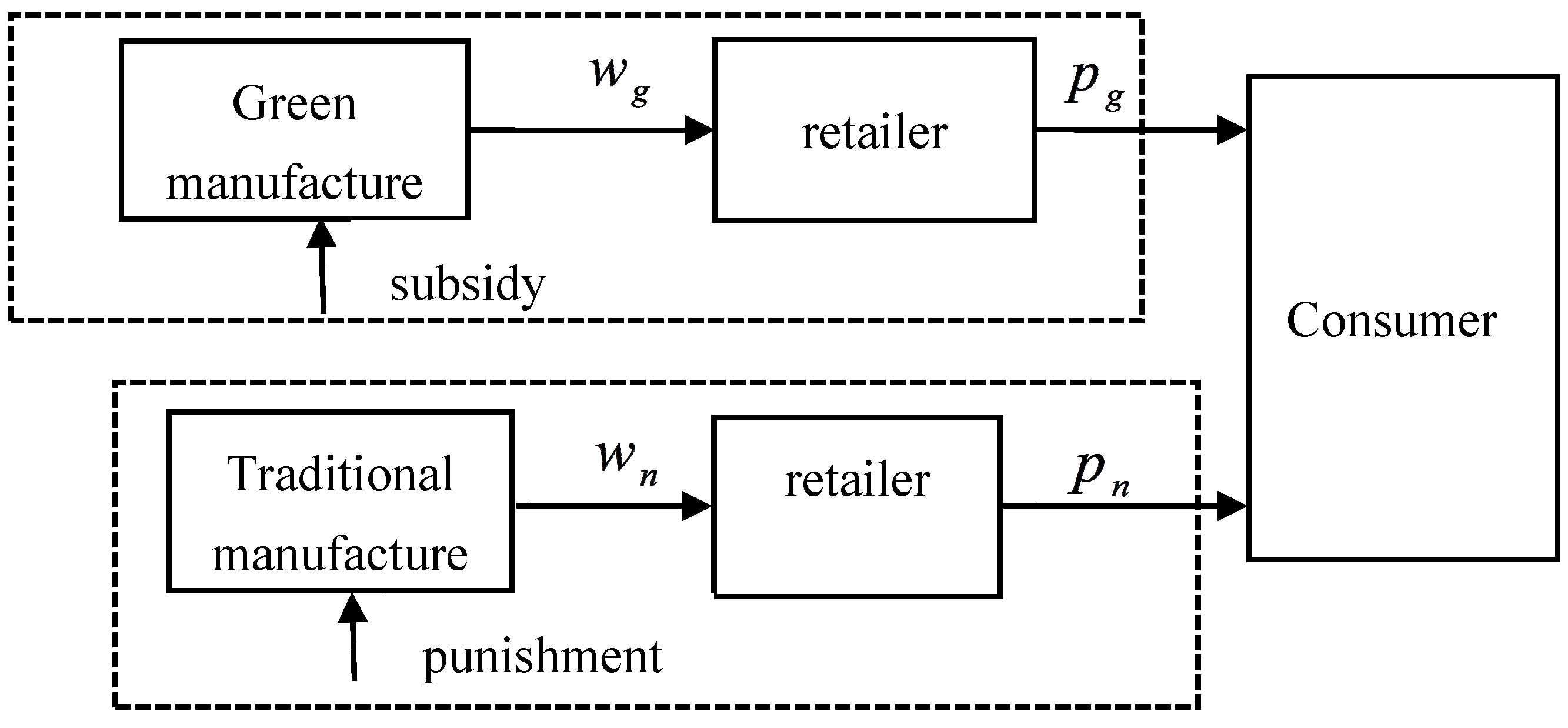
3. Problem Formulation and Notations

Consider two supply chains: the GSC and TSC. Each supply chain is composed of one manufacturer and one retailer. They produce products (green or traditional ones) and sell them to consumers through the retailer. The government adopts different policies to supply chains, provides subsidies to the GSC and punishment to the TSC. Supply chains compete on prices and the green levels of products. They have two strategies: centralized or decentralized strategies. When supply chains choose a decentralized strategy, in more cases, the manufacturer enjoys sufficient power as the channel leader who can anticipate the retailer’s response and make decisions, and the retailer is the follower. However, when supply chains choose a centralized strategy, as a whole, the manufacturer and retailer are co-determination makers.

This paper investigates the channel structure strategy of two competing supply chains (GSC and TSC). Especially, we analyze the impacts of substitutability and cost structures of products on channel structure strategy. Under different channel structure strategies, manufacturers and retailers make decisions maximizing their own or the whole supply chain’s profits. The business flow of the two supply chains competition decision is shown in Figure 1.

We have the following notations.

$p_g$, $p_t$: retail price of green and traditional products, which is a supply chain or retailer’s decision variable, $p_g$, $p_t\ge 0$;

$w_g$,: unit wholesale price of green and traditional products, which is the manufacturers’ decision variable;

$g$: green level of a product, which is the GSC or green manufacturer’s decision variable, $g\ge 0$;

$c$: marginal manufacturing cost sensitivity of a green product;

$D_g$, $D_t$: consumer demands for green and traditional products;

$\tilde{a}$: the market scale of the product;

${\lambda }_1$, ${\lambda }_2$: consumer’s sensitivity parameter of green levels to green or traditional products’ demands;

${\pi }_{gm}$, ${\pi }_{nm}$: green and traditional manufacturer’s profits;

${\pi }_{gr}$, ${\pi }_{nr}$: green and traditional retailer’s profits;

${\pi }_{gsc}$, ${\pi }_{nsc}$: the total profits of GSC and TSC, which is the sum of the manufacturer’s and retailer’s profits.

Similar to Madani and Rasti-Barzoki [40] and Ghosh and Shah [48], we assume that consumer demands are dependent on the retail price of the product itself, the retail price of a competing product, and the green level in a tractable form of linear expression. Specifically, consumer demands are negatively related to the retail price of the product itself but positively related to the retail price of the competing product. Similarly, the green level has a positive impact on consumer demand of green products, but a negative impact on the demand of a traditional one. Consumer demands are as follows

$$D_g=a_g-p_g+b{p}_n+{\lambda }_{1}g$$

(1)

$$D_t=a_t-p_t+b{p}_g-{\lambda }_{2}g$$

(2)

where $a_g=\rho a$, $a_t=(1-\rho )a$ are basic market sizes of green and traditional products. $\rho$ is consumer loyalty to GSC, $0\le \rho \le 1$. $b$ is sensitivity coefficient of the cross-price to consumer demands, $0\le b\le 1$. ${\lambda }_1>{\lambda }_2$ reflects that the impact of green level on green product’s demand is greater than the demand for traditional products.

This demand function assumption is different from Li and Li [27], in which the prices of competing products are given and the same. This assumption is also different from Bian et al. [34], in which consumer demand is assumed to be the function of retail price only and the manufacturer’s environmental concerns are expressed in the objective function by assigning a weight to the environmental damage.

For simplicity, we make the following modeling assumptions:

A1. Following Yang and Xiao [44], the government offers subsidies to green manufacturers for producing each unit green product $s=k{g}_0(g-g_0)$, where $g_0$ is the green level floor for subsidy, $k$ is the government’s adjustment factor of offering a subsidy to the green manufacturer. Taking into account many other decision factors, when $g>g_0$, the manufacturer has the behavioral tendencies to increase the subsidy; however, when $g<g_0$, the manufacturer has the behavioral tendencies to risk the punishment. For using the threshold level to represent behavioral tendency, see De et al. [49]. Especially for traditional products, since the green level is zero, according to this assumption, the government punishes by $-k{g}_0^2$ for every unit of traditional product.

Actually, a subsidy is often related to the green level $g$ and the green level floor $g_0$. Generally, a green level floor $g_0$ for subsidy is also needed. According to government policy, the higher the green level $g$, the more the subsidy $s$ will be. For example, in the standard of energy-saving air conditioning, there are 500–850 and 300–650 CNY subsidy to per unit of energy-saving air conditioning of primary and secondary levels, respectively (National development and reform commission of the People’s Republic of China. Available online: http://xwzx.ndrc.gov.cn/mtfy/dfmt/200907/t20090728_293093.html). In addition, when the total subsidy is certain, if the government raises the green level floor of subsidy, which means that less air conditioners can obtain the subsidy, the unit subsidy rises consequently. For traditional products, because of the relatively higher environmental cost, the government collects fixed taxation generally.

A2. The cost of a green manufacturer consists of two parts: the fixed investment cost $I$ and the marginal manufacturing cost $C$. They are both positively related to the green level $g$. Similar to Banker et al. [50], we assume $I=\mu g^2/2$. The fixed investment cost $I$ increases and is convex to the green level $g$, which means that when the green level is relatively high, green manufacturing becomes more difficult. $\mu$ is the marginal investment cost when the green product is at a unit of green level. Following Yang et al. [51], raw materials play a vital role in a green product’s manufacturing process, that is, the higher the green level, the higher the cost of raw materials, and the higher the marginal cost of the product. Accordingly, we assume $C=cg$, where $c$ is the increase in the manufacturing cost when the green manufacturer improves the green level by one unit. For example, green furniture manufacturers often purchase wood from regenerate forests. Moreover, green clothing manufacturers use organic cotton as raw material [46]. This assumption considers the additional cost caused by the improvement of green levels, which is different from most studies such as Zhang et al. [17], Li and Li [27], Xing et al. [33], and Bian et al. [34] where they have assumed that manufacturing cost is a fixed and given parameter.

From the above description and analyses, the membership profits of the competing supply chains are as follows:

$${\pi }_{gm}=(w_g-cg+k{g}_0(g-g_0))D_g-\frac{\mu g^2}{2}$$

(3)

$${\pi }_{gr}=(p_g-w_g)D_g$$

(4)

$${\pi }_{tm}=(w_t-k{g}_0^2)D_t$$

(5)

$${\pi }_{tr}=(p_t-w_t)D_t$$

(6)

The channel total profits of the competing supply chains can be written as

$${\pi }_{gsc}=(p_g-cg+k{g}_0(g-g_0))D_g-\frac{\mu g^2}{2}$$

(7)

$${\pi }_{tsc}=(p_t-k{g}_0^2)D_t$$

(8)

Before analyzing the Nash equilibrium of channel structure strategies, we first explain the concept of Nash equilibrium. In a game, no matter what the other party’s strategy is, each party will choose a certain strategy, called the dominant strategy. If the combination of the strategies of two players in a game constitutes their respective dominant strategies, the combination of these two strategies is defined as a Nash equilibrium (reference). In our context, the channel structure strategy has two options: centralization and decentralization. Two supply chains can choose either option, which gives rise to four channel structure scenarios.

In the following, we first study the pricing and green level decisions and profits under the four channel structure scenarios, respectively. Then we examine the impact of the competition between green and traditional products on the equilibrium outcomes. Finally, we give numerical examples to generate more managerial insights.

4. Equilibrium Strategies Analyses under Different Channel Structure Scenarios with Exogenous Green Level

In this section, we investigate equilibrium prices and profits under four channel structure models (CC, DD, DC, and CD scenarios) when the green level is exogenous. We use superscript $i$ to represent the equilibrium outcomes under model $i$, $i=CC,DD,DC,\mathrm{and}CD$. Further, we compare the equilibrium profits under different channel structure scenarios and obtain Nash equilibrium strategies, optimal prices and green levels, and its conditions.

4.1. Equilibrium Decisions under the CC Scenario

When the two competing supply chains both choose a centralized structure, they set their retail prices to maximize the channels’ profits simultaneously.

The game model can be solved by using the backwards induction. From Equations (7) and (8), we can derive Proposition 1. See Appendix A.

Proposition 1.

Under the CC scenario, the equilibrium decisions are as follows:

$$p_g^{CC*}=\frac{(2\rho +b(1-\rho ))a+(2c+2{\lambda }_1-b{\lambda }_2-2k{g}_0)g+B_{00}}{4-b^2}$$

$$p_t^{CC*}=\frac{(b\rho +2(1-\rho ))a+(bc+b{\lambda }_1-2{\lambda }_2-bk{g}_0)g+B_{00}}{4-b^2}$$

where$B_{00}=(2+b)k{g}_0^2$.

Proposition 1 shows the green and traditional supply chains’ pricing decisions in the CC scenario. From the results, we can intuitively obtain that GMMC has a positive impact on the green product’s retail price. Unexpectedly but interestingly, GMMC also has a positive impact on the retail price of the traditional product. This is possibly because the competitiveness between supply chains makes the traditional supply chain increase its retail price when the green product’s retail price is relatively high.

Substituting the equilibrium decisions obtained from Proposition 1 into Equations (7) and (8), the profits of GSC and TSC (${\pi }_{gsc}(p_g^{*},p_t^{*})$ and ${\pi }_{tsc}(p_g^{*},p_t^{*})$) under the centralized structure can be obtained, simplified them as ${\pi }_{gsc}^{VV*}$ and ${\pi }_{tsc}^{VV*}$.

4.2. Equilibrium Decisions under the DD Scenario

Under the DD scenario, the time sequence of this game is as follows:

(i) Manufacturers of the two supply chains announce their wholesale prices of green or traditional products simultaneously.

(ii) After observing the wholesale prices, retailers of the two supply chains announce their retail prices of green or traditional products.

From Equations (3)–(6), using the backwards induction, we can derive Proposition 2.

Proposition 2.

Under the DD scenario, the equilibrium decisions are as follows:

(a) The wholesale prices are

$$w_g^{DD*}=\frac{B_{10}+B_{11}b++B_{12}{b}^2+B_{13}{b}^3+B_{14}{b}^4}{16-17b^2+4b^4}$$

$$w_t^{DD*}=\frac{B_{20}+B_{21}b+B_{22}{b}^2+B_{23}{b}^3+B_{24}{b}^4}{16-17b^2+4b^4}$$

(b) The retail prices of green and traditional products are

$$p_g^{DD*}=\frac{1}{(-4+b^2)}\left(\frac{2B_{10}+b(2B_{11}+B_{20})+b^2(2B_{12}+B_{21})+b^3(2B_{13}+B_{22})+b^4(2B_{14}+B_{23})+b^5{B}_{24}}{(16-17b^2+4b^4)}\right)$$

$$p_t^{DD*}=\frac{1}{(-4+b^2)}\left(\frac{2B_{10}+b(B_{10}+2B_{21})+b^2(B_{11}+2B_{22})+b^3(B_{12}+2B_{23})+b^4(B_{13}+2B_{24})+b^5{B}_{14}}{(16-17b^2+4b^4)}\right)$$

where$B_{10}=8(a\rho +cg-g{g}_{0}k+g_0^{2}k-g{\lambda }_1)$,$B_{11}=6a(1-\rho )+2g_0^{2}k-6g{\lambda }_2$,

$B_{12}=-3a\rho -8cg+8g{g}_{0}k-8g_0^{2}k-3g{\lambda }_1$,$B_{13}=-2a(1-\rho )-g_0^{2}k-2g{\lambda }_2$,$B_{14}=2cg-2g{g}_{0}k+2g_0^{2}k$,

$B_{20}=8(a(1+\rho )+g_0^{2}k-g{\lambda }_2)$,$B_{21}=6a\rho +2(cg-g{g}_{0}k+g_0^{2}k+3g{\lambda }_1)$,

$B_{22}=-3a(1-\rho )-8g_0^{2}k+3g{\lambda }_2$,$B_{23}=-2a\rho -cg+g{g}_{0}k-g_0^{2}k-2g{\lambda }_1$,$B_{24}=2g_0^{2}k$.

Substituting the equilibrium decisions obtained from Proposition 2 into Equations (3)–(6), profits of manufacturers and retailers of GSC and TSC under MM structure can be obtained. Further, the channel total profits of supply chains are obtained, simplified them as ${\pi }_{gsc}^{DD*}$ and ${\pi }_{tsc}^{DD*}$.

4.3. Equilibrium Decisions under the DC Scenario

Under the DC scenario, the time sequence of this game is as follows:

(i) The green manufacturer announces the green product’s wholesale price; meanwhile, the traditional manufacturer and the retailer of TSC announce the retail price of the traditional product simultaneously.

(ii) After observing the green product’s wholesale price and the traditional product’s retail price, the retailer of GSC announces the retail price of the green product.

From Equations (3), (4), and (8), we derive the following:

Proposition 3.

Under the DC scenario, the equilibrium decisions are as follows:

(a) The retail prices of green and traditional products are

$$p_g^{DC*}=\frac{1}{4-b^2}(\frac{B_{30}+B_{31}b-B_{32}{b}^2}{2(2-b^2)}+(2+b(1-\rho ))a+(2{\lambda }_1-b{\lambda }_2)g+bk{g}_0^2)$$

$$p_n^{DC*}=\frac{1}{4-b^2}(\frac{b(B_{30}+B_{31}b-B_{32}{b}^2)}{2(2-b^2)}+(b\rho +2(1-\rho ))a+(b{\lambda }_1-2{\lambda }_2)g+2k{g}_0^2)$$

(b) Green product’s equilibrium wholesale price is

$$w_g^{DC*}=\frac{B_{30}+B_{31}b+B_{32}{b}^2}{2(2-b^2)}$$

where$B_{30}=2\left(a\rho +cg-g{g}_{0}k+g_0^{2}k+g{\lambda }_1\right)$,$B_{31}=a(1-\rho )+g_0^{2}k-g{\lambda }_2$,$B_{32}=2\left(g{g}_{0}k-cg-g_0^{2}k\right)$

4.4. Equilibrium Decisions under the CD Scenario

Under the CD scenario, the time sequence of this game is as follows:

(i) GSC announces the retail price of the green product; meanwhile, the traditional manufacturer announces the wholesale price of the traditional product.

(ii) After observing the retail price of the green product and the wholesale price of the traditional product, the retailer of TSC announces the retail price of the traditional product.

From Equations (5)–(7), we derive the following proposition.

Proposition 4.

Under the CD scenario, the equilibrium decisions are as follows:

(a) The retail prices of green and traditional products are

$$p_g^{CD*}=\frac{1}{4-b^2}(\frac{b(B_{40}+b{B}_{41}+b^2{B}_{42})}{2(2-b^2)}+(b+(2-b)\rho )a+(2{\lambda }_1-b{\lambda }_2)g+2cg-2kg{g}_0+2k{g}_0^2)$$

$$p_n^{CD*}=\frac{1}{4-b^2}(\frac{b(B_{40}+b{B}_{41}+b^2{B}_{42})}{2(2-b^2)}+(b\rho +2(1-\rho ))a+bcg+(b{\lambda }_1-2{\lambda }_2)g-bg{g}_{0}k+bk{g}_0^2)$$

(b) The traditional product’s equilibrium wholesale price is

$$w_g^{MV*}=\frac{B_{40}+B_{41}b+B_{42}{b}^2}{2(2-b^2)}$$

where $B_{40}=2\left(a(1-\rho )-g_0^{2}k-g{\lambda }_2\right)$, $B_{41}=a\rho +cg-g{g}_{0}k+g_0^{2}k+g{\lambda }_1$, $B_{42}=-g_0^{2}k$.

Combining the results of Propositions 1–4, we know that the equilibrium wholesale and retail prices are dependent on the competitive degree between supply chains. Then, in next subsection, we mainly investigate the effect of competitive degree on channel structure strategy.

4.5. Channel Structure Strategies Analyses

This subsection compares and analyzes the equilibrium results obtained in Section 4.1, Section 4.2, Section 4.3 and Section 4.4 under different channel structures of the two supply chains, and obtains the equilibrium channel structure of the two supply chains and the key influencing factors. Further, some important management implications are derived.

Proposition 5.

${\pi }_{gsc}^{CC*}>{\pi }_{gsc}^{DC*}$, ${\pi }_{nsc}^{CC*}>{\pi }_{nsc}^{CD*}$.

From Proposition 5, we know that when TSC chooses a centralized strategy, GSC also chooses a centralized strategy, and vice versa. That is, for any product competition degree, government policy and GMMC, CC is always the Nash equilibrium. This finding is consistent with Wu et al. [21], who insist that CC is the unique Nash equilibrium over one period decision. In practice, a few supply chains do adopt some coordination mechanisms to induce the supply chain to act as if they are vertically integrated, such as buy-back, revenue sharing, and quantity flexibility.

Proposition 6.

If $0\le b\le b_1$, then ${\pi }_{gsc}^{DD*}\le {\pi }_{gsc}^{CD*}$, ${\pi }_{nsc}^{DD*}\le {\pi }_{nsc}^{DC*}$;

If $b_1<b\le 1$, then ${\pi }_{gsc}^{DD*}>{\pi }_{gsc}^{CD*}$, ${\pi }_{nsc}^{DD*}>{\pi }_{nsc}^{DC*}$.

According to Proposition 6, the following results can be drawn. If GSC chooses a decentralized strategy, TSC’s strategy depends on the substitutability of products. Specifically, when substitutability of products is relatively small, concentration is a better strategy. However, when substitutability of products is relatively large, a decentralized strategy is better, and vice versa. That is, given one supply chain chooses a decentralized strategy, the other supply chain’s strategy is dependent on the competition degree of the supply chains. This result is consistent with Wu et al. [21] but different from Zhang et al. [17]. Zhang et al. [17] insisted that cooperation is always better than non-cooperation. This is possibly because Zhang et al. [17] considered a single green supply chain with a hybrid production mode. However, Wu et al. [22] showed that DD may also be at Nash equilibrium over infinitely many periods. Practically, decentralized supply chains have been commonly observed in a broad range of industries, such as electronics, pharmaceuticals, and automotive (Zhao and Shi [31]).

From above analyses, if the competition degree of supply chains is relatively small (represented by the value of b), CC is the unique Nash equilibrium. However, if the competition degree of supply chains is relatively large, CC and DD are both the Nash equilibriums regardless of government intervention and other factors.

This section mainly discusses equilibrium decisions and strategies of competing supply chains under different conditions with an exogenous green level, especially, the effect of product competitive degree on Nash equilibriums. For investigating the effect of other key factors on channel structure strategy, in the following section, channel structure scenarios with endogenous green levels will be considered.

5. Equilibrium Analyses under Different Channel Structure Scenarios with Endogenous Green Levels

In this section, we investigate equilibrium decisions under different channel structure scenarios when the green level is endogenous, respectively. Further, numerical analyses compare the equilibrium profits, prices, and green levels under different scenarios, and obtain channel structure strategies with respect to government policy and GMMC.

5.1. Equilibrium Decisions under Different Channel Structure Scenarios

When the green level is endogenous, it is a decision variable. In this subsection, we analyze the equilibrium decisions of different channel structures.

Under the CC scenario, GSC sets the retail price of the green product and the green level, and TSC sets retail price of the traditional product to maximize their channels’ profits simultaneously.

From Equations (7) and (8), we can derive Proposition 7.

Proposition 7.

Under the CC scenario, if $\mu >{\mu }_1$ ($\mu$ is a green product’s marginal investment cost at unit green level), there exists optimal equilibrium decisions $\left(p_g^{CC*},g^{CC*},p_t^{CC*}\right)$, where ${\mu }_1=\frac{{({\lambda }_1+kg)}^2}{2}$.

The assumption $\mu >{\mu }_1$ ensures the existence and uniqueness of the Nash equilibrium, which is critical for yielding an analytically tractable solution. Thus, in analyzing the CC scenario, we assume that the condition $\mu >{\mu }_1$ is always satisfied.

Under the DD scenario, the time sequence is as follows: First, the green manufacturer sets the wholesale price of the green product and the green level, and the traditional manufacturer sets the wholesale price of the traditional product to maximize their profits simultaneously. Then, the retailers of the two supply chains set the retail prices of products.

From Equations (3)–(6), we derive Proposition 8.

Proposition 8.

Under the DD scenario, if $\mu >{\mu }_2$, there exist optimal equilibrium decisions $\left(p_g^{DD*},p_t^{DD*},w_g^{DD*},w_t^{DD*},g^{DD*}\right)$, where ${\mu }_2=\frac{{(2{\lambda }_1+b{\lambda }_2+k{g}_0(2-b^2))}^2}{2(2-b^2)(4-b^2)}$.

Similar to Proposition 7, the assumption $\mu >{\mu }_2$ ensures the existence and uniqueness of the Nash equilibrium of DD scenario.

Under the DC scenario, the time sequence is as follows: First, the green manufacturer sets the wholesale price of the green product and the green level. Then, the retailer of GSC sets the retail price of the green product, and TSC sets the retail price of the traditional product to maximize their profits simultaneously.

From Equations (3), (4), and (8), we can derive Proposition 9.

Proposition 9.

Under the DC scenario, if $\mu >{\mu }_2$, there exist optimal equilibrium decisions $(p_g^{DC*},p_t^{DC*},w_g^{DC*},g^{DC*})$, where ${\mu }_1$ is given in Proposition 7.

Under DC scenario, the time sequence is as follows: First, the traditional manufacturer sets the wholesale price of the traditional product. Then, the retailer of TSC sets the retail price of the traditional product, and GSC sets the green level and the retail price of the green product to maximize their profits.

From Equations (3)–(6), we can derive Proposition 10.

Proposition 10.

Under the CD scenario, if $\mu >{\mu }_1$, there exist optimal equilibrium decisions $(p_g^{CD*},g^{CD*},p_t^{CD*},w_n^{CD*})$, where ${\mu }_2$ is given in Proposition 8.

Based on the derived equilibrium solutions, qualitative and quantitative analyses are conducted in the next subsection to provide additional insights into the influence of government interventions and GMMC on channel structure strategies of green and traditional supply chains.

5.2. Channel Structure Strategy Analysis

Because of the complication of the equilibrium solutions, it is difficult to analyze their relationships analytically. In order to get more management implications, a numerical example is adopted to further analyze the channel structure strategies of the competing supply chains when the green level is endogenous. The influence of some key factors, such as government intervention policy, GMMC, and DSGL on equilibrium decisions and channel structure strategy are discussed.

We assume that the parameters are as follows: $a=10$, $b=0.77$, $\mu =2$, and $\rho =0.6$. The effect of governmental intervention on channel structure strategy is first investigated.

5.2.1. Analysis of Impact of Governmental Intervention on Equilibrium Decisions and Profits

The government sets intervention policies by green level floor $g_0$ and adjustment factor $k$. We first investigate the impacts of green level floor $g_0$ on channel structure strategy by analyzing profits of the GSC and TSC under different governmental interventions.

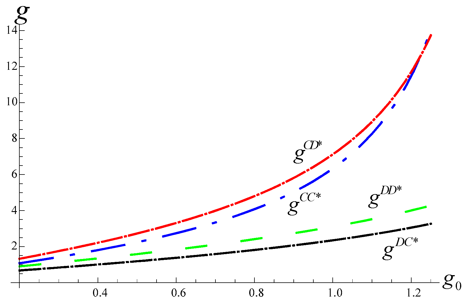
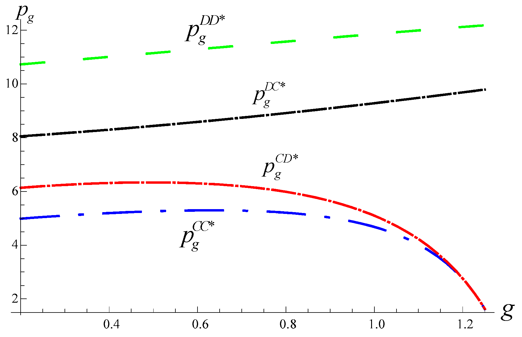
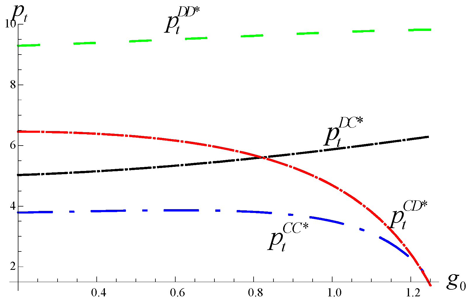
If $c=0.5$, ${\lambda }_1=0.7$, ${\lambda }_2=0.3$, $k=1.2$, then, from the above discussion in this section, the green level floor range is $0\le g_0<1.25$. For comparison and analysis, we draw graphs of retail prices, green levels, and profits of the two supply chains under four structure scenarios, as shown in Figure 2, Figure 3, Figure 4, Figure 5 and Figure 6.

From Figure 2, Figure 3 and Figure 4, we derive the following results.

Firstly, from Figure 2, it is easy to find that the green level floor has a positive impact on the green level regardless of the channel structure scenarios, which indicates that a relatively high green level floor is beneficial for the improvement of the green level. Then, the green level is also higher in centralization than decentralization for GSC. From Figure 3 and Figure 4, the impacts of the green level floor on the retail prices of both green and traditional products depend on the channel structure. Interestingly, it displays that the retail prices of both green and traditional products increase with the green level floor when GSC is in a decentralized structure, but decrease when GSC is in a centralized structure. Moreover, when the green level floor is relatively low, we have $p_t^{DD*}>p_t^{CD*}>p_t^{DC*}>p_t^{CC*}$, and when green level floor is relatively high, we have $p_t^{DD*}>p_t^{DC*}>p_t^{CD*}>p_t^{CC*}$. As for the green product, for any green level floor, we have $p_g^{DD*}>p_g^{DC*}>p_g^{CD*}>p_g^{CC*}$.

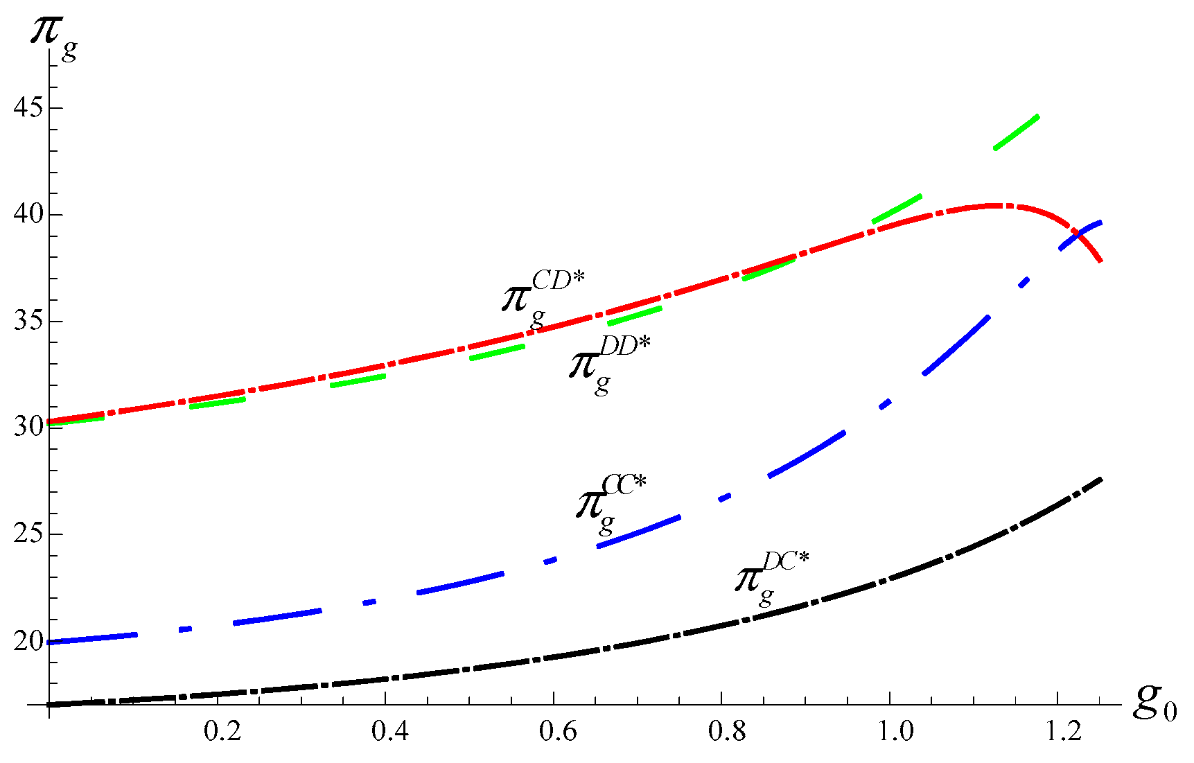
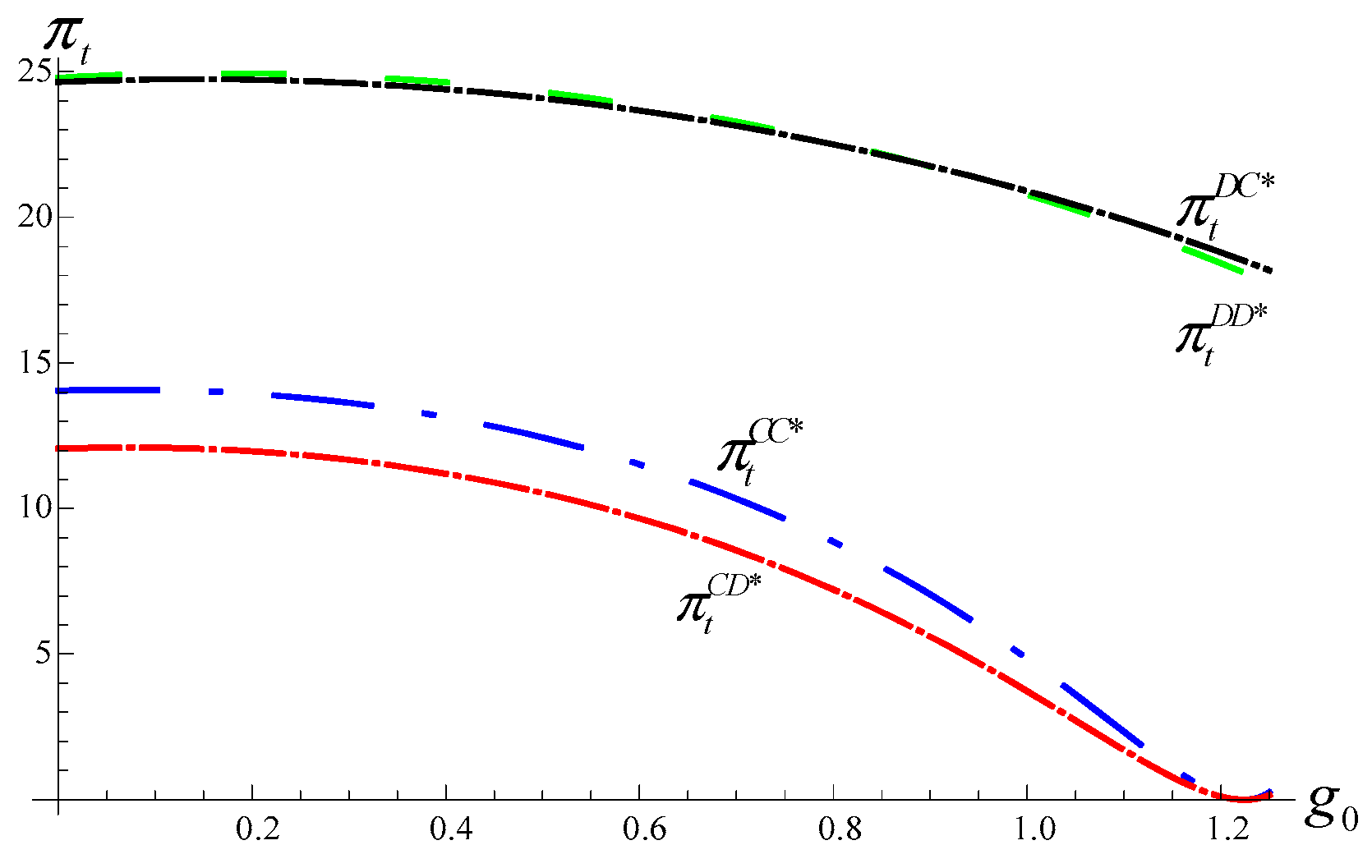
Secondly, the green level floor has a positive impact on the profits of GSC but a negative impact on TSC generally. Then from Figure 5, for GSC, when green level floor is relatively low, we have the following results: ${\pi }_{gsc}^{CD*}$ $>{\pi }_{gsc}^{DD*}$ $>{\pi }_{gsc}^{CC*}$ $>{\pi }_{gsc}^{DC*}$; however, when green level floor is relatively high, we have ${\pi }_{gsc}^{DD*}>$ ${\pi }_{gsc}^{CD*}$ $>{\pi }_{gsc}^{CC*}$ $>{\pi }_{gsc}^{DC*}$. That is, when TSC is centralized, GSC will also choose centralization. But when TSC is decentralized, GSC’s choice depends on the green level floor. Specifically, when the green level floor is relatively low, centralization is a better choice, but when green level floor is relatively high, decentralization is better. Similarly, for TSC, when the green level floor is relatively low, we have ${\pi }_{tsc}^{DD*}$ $>{\pi }_{tsc}^{DC*}$ $>{\pi }_{tsc}^{CC*}>$ ${\pi }_{tsc}^{CD*}$; however, when green level floor is relatively high, we have ${\pi }_{tsc}^{DC*}>$ ${\pi }_{tsc}^{DD*}$ $>{\pi }_{tsc}^{CC*}>$ ${\pi }_{tsc}^{CD*}$. In other words, when GSC is centralized, TSC will also choose centralization. But when GSC is decentralized, GSC’s choice also depends on the green level floor. Different from GSC, a relatively low green level floor may result in a decentralized choice of TSC.

According to the above analysis, the following managerial insights are obtained:

(1.1) CC is always the Nash equilibrium. This result is consistent with Li and Li [28]. However, Nash equilibrium CC may not realize optimal green levels, but consumers can obtain the lowest retail prices from both GSC and TSC.

(1.2) The green level floor plays different roles in the channel structure choice of GSC and TSC. When the competitor is decentralized, a relatively high green level floor may result in a centralized choice of TSC but a decentralized choice of GSC. However, a relatively low green level floor may result in a decentralized choice of TSC but a centralized choice of GSC. This is an extension of the result of Li and Li [28].

For investigating the impact of adjustment factor $k$ on channel structure strategies, we assume $g_0=1$. The other parameters are same as the above. From discussion in Section 5.1, the range of adjustment factors is $0\le k\le 1.62$. Similarly, we depict the profits of the two supply chains under different structure scenarios, as shown in Figure 7 and Figure 8.

From Figure 7 and Figure 8, we can obtain the following results.

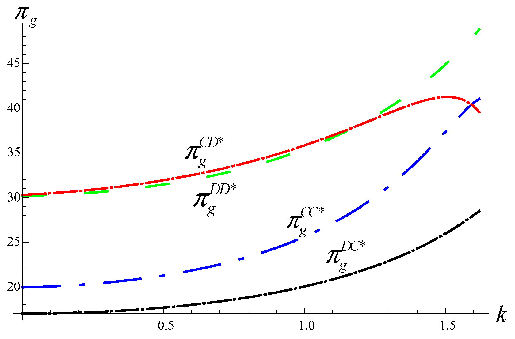
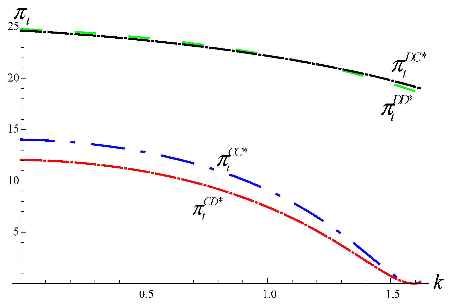
Firstly, adjustment factor $k$ has a positive impact on the profits of GSC regardless of the channel structure. But the impact of adjustment factor $k$ on TSC depends on the channel structure. When TSC is centralized, the impact is negative. Otherwise, the impact is positive. This finding is different from Madani and Rasti-Barzoki [40], who consider that the government tax rate always decreases the profit of the TSC. This is because Madani and Rasti-Barzoki [40] did not consider the channel structure in their model. Then, neither GSC nor TSC can maximize their own profit in Nash equilibrium CC. In Nash equilibrium DD, whether the GSC and the TSC can realize their optimal profits depends on the adjustment factor. When the adjustment factor is relatively low, we have the following results: ${\pi }_{gsc}^{CD*}$ $>{\pi }_{gsc}^{DD*}$ $>{\pi }_{gsc}^{CC*}$ $>{\pi }_{gsc}^{DC*}$ and ${\pi }_{tsc}^{DD*}$ $>{\pi }_{tsc}^{DC*}$ $>{\pi }_{tsc}^{CC*}>$ ${\pi }_{tsc}^{CD*}$, but when the adjust factor is relatively high, we have ${\pi }_{gsc}^{DD*}>$ ${\pi }_{gsc}^{CD*}$ $>{\pi }_{gsc}^{CC*}$ $>{\pi }_{gsc}^{DC*}$ and ${\pi }_{tsc}^{DC*}>$ ${\pi }_{tsc}^{DD*}$ $>{\pi }_{tsc}^{CC*}>$ ${\pi }_{tsc}^{CD*}$. It means that when the competitor is decentralized, both GSC and TSC’s optimal choice is related to the adjustment factor. A relatively high adjustment factor may make GSC choose a decentralized structure, but make TSC choose a centralized structure.

From the analysis, some managerial insights can be obtained:

(1.3) Adjustment factor $k$ plays a vital role in channel structure strategy of both GSC and TSC when the opposite is decentralized. If the adjustment factor is relatively high, a decentralized structure is a better choice for GSC, but if the adjust factor is relatively low, centralization is better for GSC. As for TSC, the choice is the opposite.

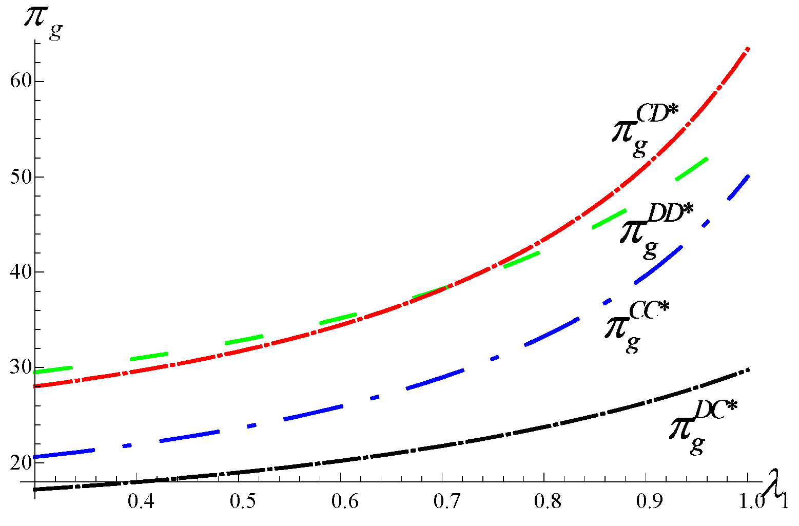
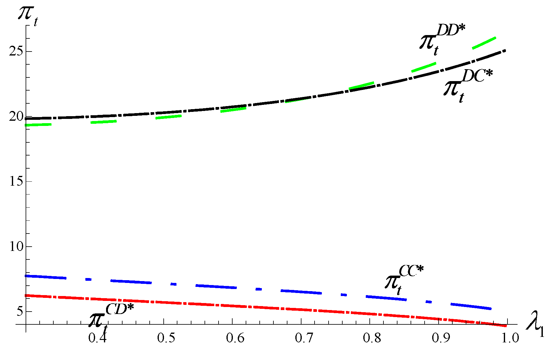
5.2.2. Analysis of Impact of GMMC on Equilibrium Decisions and Profits

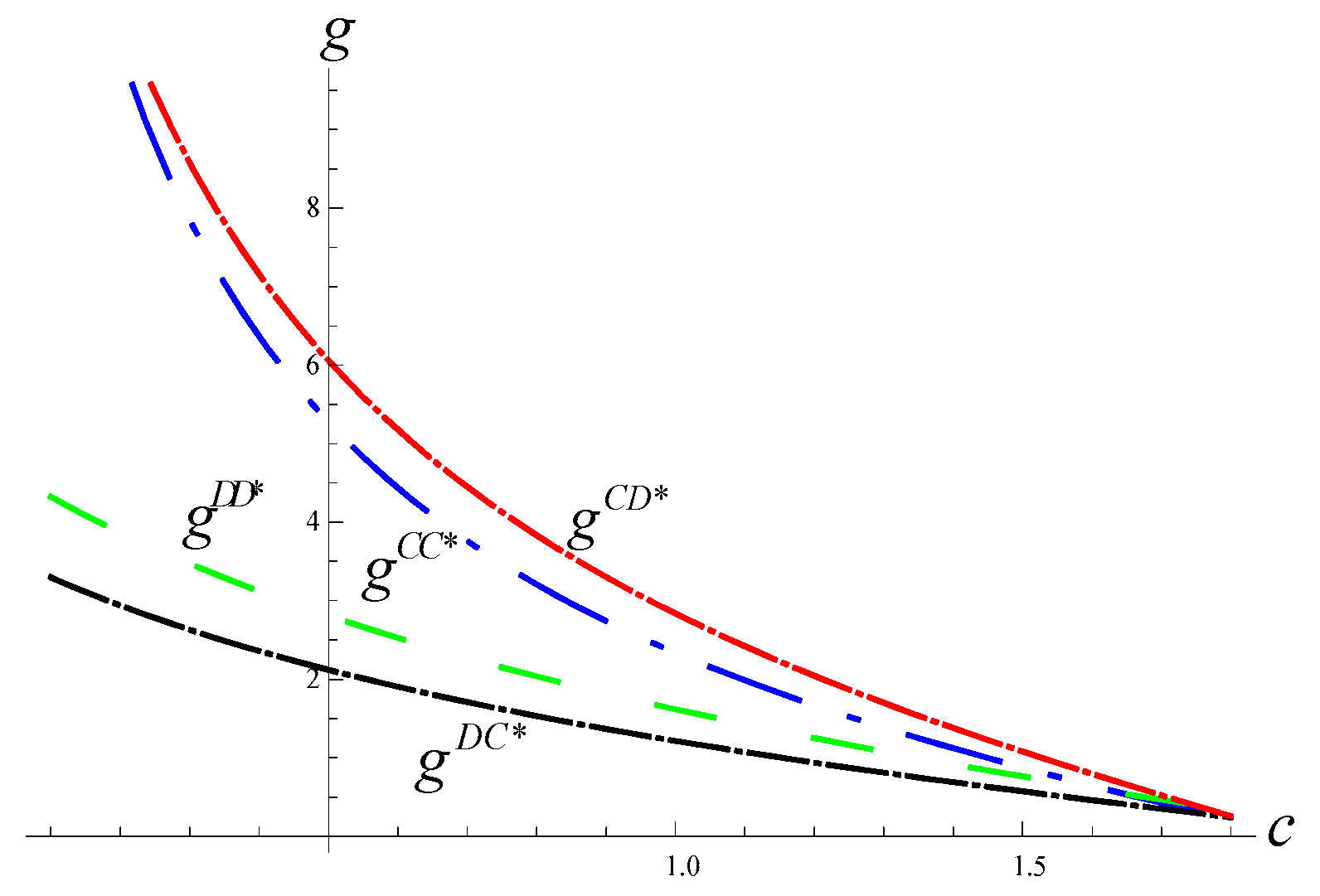
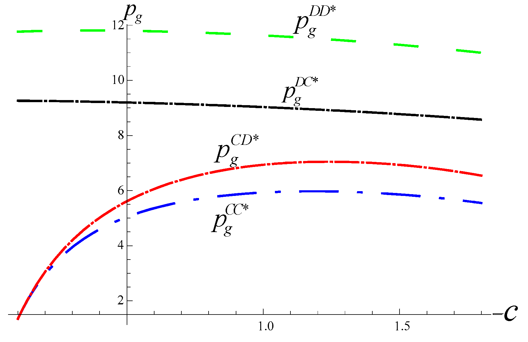
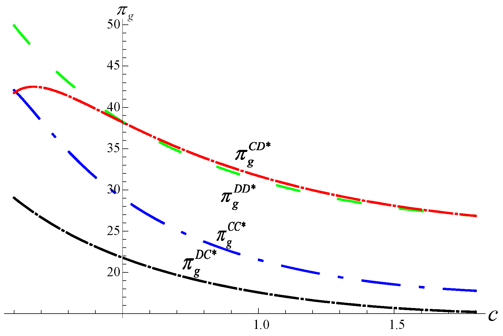
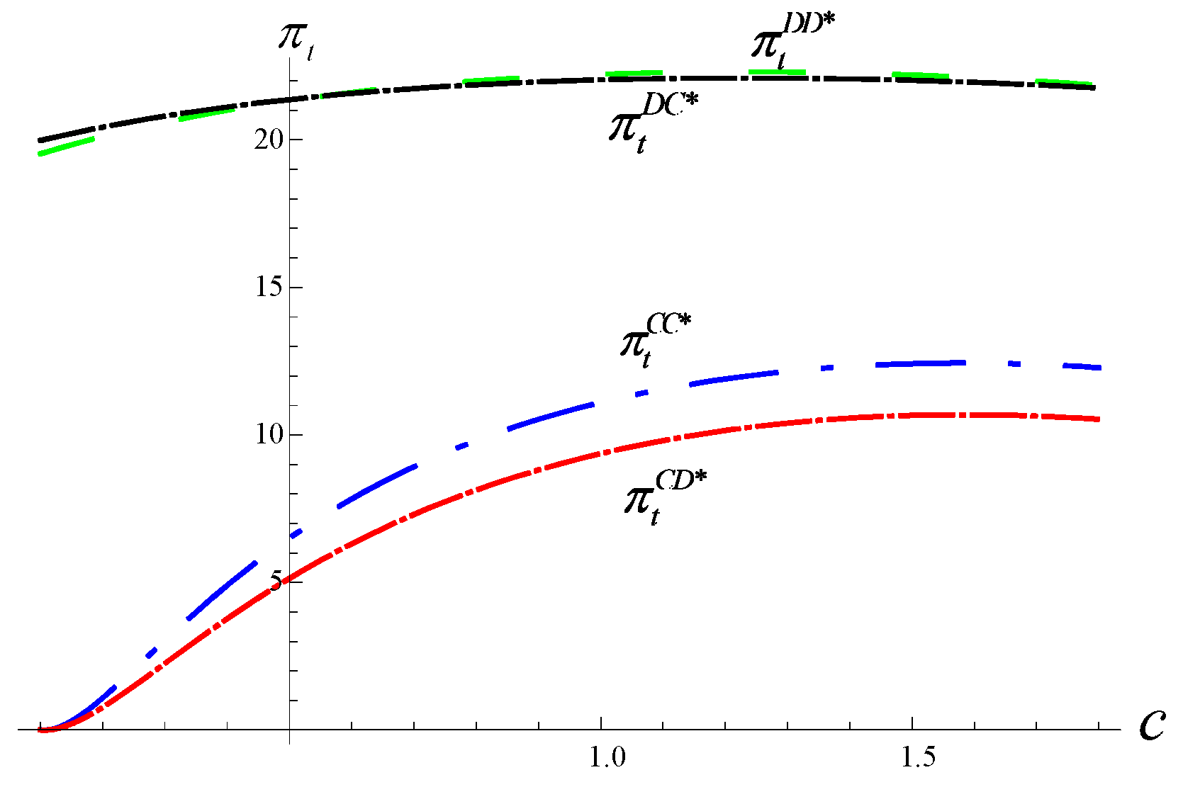
In this subsection, we analyze the impact of GMMC (green marginal manufacturing cost) on the equilibrium decisions and channel structure strategy. We consider the difference in retail prices, green levels, and the profits of GSC and TSC under different channel structure scenarios when GMMC varies and when governmental intervention is as follows: $g_0=1$, $k=1.2$. The other parameters are as same as those in Section 5.2.1. The change of the key variables and the expected profits are shown in Figure 9, Figure 10, Figure 11 and Figure 12.

Remark 1.

The following results can be obtained from Figure 9, Figure 10, Figure 11 and Figure 12:

(1) From Figure 9 and Figure 10, the GMMC has a negative impact on green levels, which is an intuitive result. But counter-intuitively, different from the centralized scenario, when GSC is decentralized, the retail price of the green product decreases slightly with the GMMC. This is possibly because decentralization increases the competitiveness of GSC.

(2) From Figure 11 and Figure 12, it is straightforward that GMMC has a negative impact on GSC but a positive impact on TSC. In other words, a relatively high GMMC is unfavorable for GSC in competition. In addition, when the competitor is centralized, the effect of the GMMC on channel structure strategy may not be evident for the two supply chains. However, when the competitor is decentralized, both GSC and TSC’s strategies are dependent on the GMMC. Specifically, when the competitor is decentralized, if the GMMC is relatively low, the GSC’s best choice may also be decentralization; if the GMMC is relatively high, the GSC’s best choice would be centralization. From Figure 12, the impact of the GMMC on TSC’s channel structure strategy may be just the opposite to its impact on TSC.

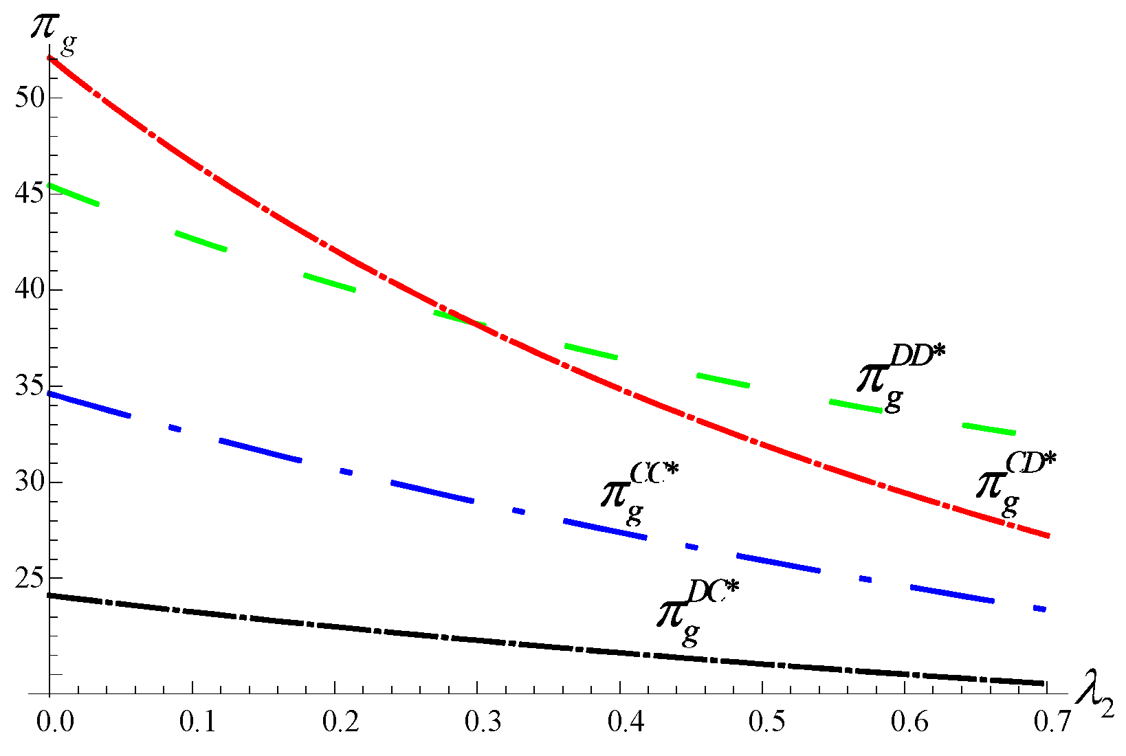
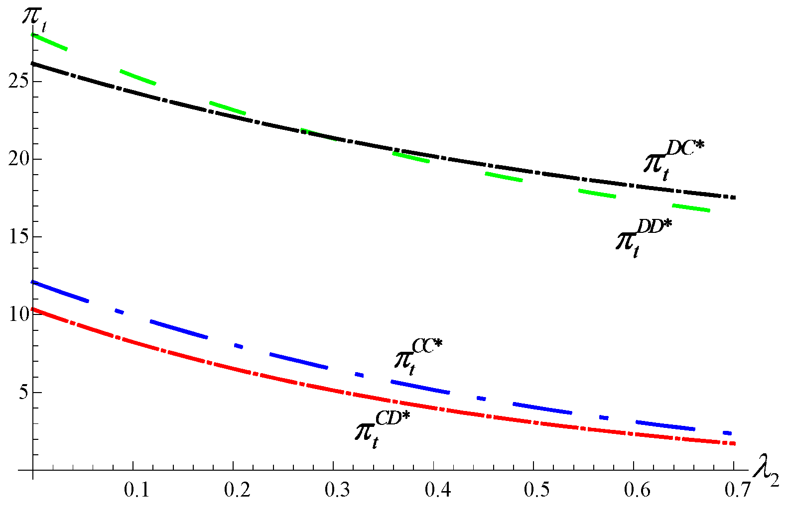
5.2.3. Analysis of Impact of DSGLs on Equilibrium Profits

In this subsection, we want to analyze the influence of DSGLs. We examine the impact of DSGLs on equilibrium outcomes and profits of supply chains under the four channel structure scenarios. We vary green and traditional products’ DSGLs, ${\lambda }_1$ and ${\lambda }_2$, and take the other parameters as in Section 5.2.1. The change of key variables and the profits are shown in Figure 13, Figure 14, Figure 15 and Figure 16.

Remark 2.

The following results can be obtained from Figure 13, Figure 14, Figure 15 and Figure 16:

(1) From Figure 13 and Figure 14, the DSGL ${\lambda }_1$ has a positive impact on GSC regardless of the channel structure; however, the impact of the DSGL ${\lambda }_1$ on TSC depends on the channel structure. Specifically, when the GSC is decentralized, the higher the DSGL ${\lambda }_1$, the more the TSC’s profit. When the GSC is centralized, the higher the DSGL ${\lambda }_1$, the less the TSC’s profit. In addition, the DSGL ${\lambda }_1$ has an important impact on both the GSC and the TSC’s channel structure strategies. From Figure 13, it is obtained that when TSC is decentralized, a relatively low DSGL ${\lambda }_1$ may prompt GSC to choose a decentralization strategy; however, a relatively high DSGL ${\lambda }_1$ may make GSC tend to centralization. An opposite choice can be obtained for the TSC from Figure 14.

(2) From Figure 15 and Figure 16, the DSGL ${\lambda }_2$ has a negative impact on both GSC and TSC’s profits. However, the DSGL ${\lambda }_2$ also plays an important role on the GSC and the TSC’s channel structure strategies. Different from DSGL ${\lambda }_1$, when TSC is decentralized, a relatively low DSGL ${\lambda }_2$ may make GSC prefer centralization; however, a relatively high DSGL ${\lambda }_2$ may make GSC prefer decentralization. Similar results for TSC can be observed from Figure 16.

6. Conclusions

This paper investigates the competition between GSC and TSC, considering the influence of government intervention and GMMC on channel competition and channel strategy. By analyzing four game theoretical models corresponding to different combinations of channel structure strategies for two supply chains, this paper discusses channel structure strategy and the key influential factors under the competition of GSC and TSC and governmental interventions with both endogenous and exogenous green degrees and further analyzes the condition of the equilibrium channel strategy being the optimal strategy. Some managerial insights are generated.

6.1. Managerial Implications

There are four important managerial implications as follows: Firstly, competition degree of supply chains affects the equilibrium results, and further affect the channel structure strategy. For both GSC and TSC, if any one is centralized, the competitor will also choose a centralized strategy. But when any of them is decentralized, the competitor’s strategy depends on the competition degree of the supply chains. Further, when the competition degree is weak, CC is the only Nash equilibrium. But when the competition degree is relatively severe, DD is also the Nash equilibrium. Secondly, the GMMC and DSGLs are also important factors affecting the channel structure strategy of the competing supply chains. Thirdly, whether the Nash equilibrium channel strategy is the optimal strategy for both supply chains depends on government intervention policy. When the competition degree and the governmental intervention policy are relatively severe, although CC is always the Nash equilibrium of the game, it cannot make either party reach optimal profit. Hence, CC is a prisoner’s dilemma. However, DD can make the GSC achieve its maximum profit. Fourthly, from the consumers’ viewpoint, a CD strategy can achieve the highest green level, while a DC strategy can only achieve the lowest green level. In addition, relatively severe governmental interventions might achieve the maximum green level but may not realize the lowest retail price.

6.2. Limitations and Directions for Further Research

While this work adds to the growing literature on the GSCM by integrating governmental intervention and channel competition into the models, there are also certain limitations due to some assumptions. In reality, the demand function is more complex, especially considering the green level and competition of the products. Our model may be extended to other forms of demand functions, such as the product form in Choi [5]. We assume that there is one supply chain in both GSC and TSC. Another extension is to examine the cases with multi-channels marketing on both green and traditional products. Moreover, this work assumes deterministic demand and cost; an extension to uncertain cases through chance-constrained programming or stochastic programming deserves more research. This paper mainly employs analytical methods, which may be difficult to apply to complex game models. In such cases, an evolutionary game theoretic approach may be a good alternative to simulate complex systems, e.g., incorporating green tax, risk assessment, or social impact features with big data.

References

- Peterson, S.B.; Michalek, J.J. Cost-effectiveness of plug-in hybrid electric vehicle battery capacity and charging infrastructure investment for reducing US gasoline consumption. Energy Policy 2013, 52, 429–438. [Google Scholar] [CrossRef]
- Nakandala, D.; Lau, H.C. Innovative adoption of hybrid supply chain strategies in urban local fresh food supply chain. Supply Chain Manag. Int. J. 2019, 24, 241–255. [Google Scholar] [CrossRef]
- De, A.; Wang, J.; Tiwari, M.K. Fuel bunker management strategies within sustainable container shipping operation considering disruption and recovery policies. IEEE Trans. Eng. Manag. 2019, 1–23. [Google Scholar] [CrossRef] [Green Version]
- De, A.; Choudhary, A.; Turkay, M.; Tiwari, M.K. Bunkering policies for a fuel bunker management problem for liner shipping networks. Eur. J. Oper. Res. 2019. [Google Scholar] [CrossRef]
- Choi, S.C. Price competition in a channel structure with a common retailer. Mark. Sci. 1991, 10, 271–296. [Google Scholar] [CrossRef]
- Zhang, L.; Wang, J.; You, J. Consumer environmental awareness and channel coordination with two substitutable products. Eur. J. Oper. Res. 2015, 241, 63–73. [Google Scholar] [CrossRef]
- Lin, P.C.; Huang, Y.H. The influence factors on choice behavior regarding green products based on the theory of consumption values. J. Clean. Prod. 2012, 22, 11–18. [Google Scholar] [CrossRef]
- Yu, Y.; Han, X.; Hu, G. Optimal production for manufacturers considering consumer environmental awareness and green subsidies. Int. J. Prod. Econ. 2016, 182, 397–408. [Google Scholar] [CrossRef] [Green Version]
- Tseng, M.L.; Wang, R.; Chiu, A.S.; Geng, Y.; Lin, Y.H. Improving performance of green innovation practices under uncertainty. J. Clean. Prod. 2013, 40, 71–82. [Google Scholar] [CrossRef]
- Biswas, A.; Roy, M. Green products: An exploratory study on the consumer behavior in emerging economies of the East. J. Clean. Prod. 2015, 87, 463–468. [Google Scholar] [CrossRef]
- Fang, W.; Tang, L.; Cheng, P.; Ahmad, N. Evolution decision, drivers and green innovation performance for collaborative innovation center of ecological building materials and environmental protection equipment in Jiangsu province of china. Int. J. Envion. Res. Public Health 2018, 15, 2365. [Google Scholar] [CrossRef] [Green Version]
- Seman, N.A.; Govindan, K.; Mardani, A.; Zakuan, N.; Saman, M.Z.; Hooker, R.E.; Ozkul, S. The mediating effect of green innovation on the relationship between green supply chain management and environmental performance. J. Clean. Prod. 2019, 229, 115–127. [Google Scholar] [CrossRef]
- Yu, Y.; Zhang, M.; Huo, B. The impact of supply chain quality integration on green supply chain management and environmental performance. Total Qual. Manag. Bus. Excell. 2019, 30, 1110–1125. [Google Scholar] [CrossRef]
- Chen, D.; Ignatius, J.; Sun, D.; Zhan, S.; Zhou, C.; Marra, M.; Demirbag, M. Reverse logistics pricing strategy for a green supply chain: A view of customers’ environmental awareness. Int. J. Prod. Econ. 2019, 217, 197–210. [Google Scholar] [CrossRef] [Green Version]
- Ghosh, D.; Shah, J. Supply chain analysis under green sensitive consumer demand and cost sharing contract. Int. J. Prod. Econ. 2015, 164, 319–329. [Google Scholar] [CrossRef]
- Chen, Y.; Zhang, R.; Liu, B. Joint decisions on production and pricing with strategic consumers for green crowdfunding products. Int. J. Environ. Res. Public Health 2017, 14, 1090. [Google Scholar] [CrossRef] [PubMed] [Green Version]
- Zhang, C.T.; Wang, H.X.; Ren, M.L. Research on pricing and coordination strategy of green supply chain under hybrid production mode. Comput. Ind. Eng. 2014, 72, 24–31. [Google Scholar] [CrossRef]
- Jian, J.; Guo, Y.; Jiang, L.; An, Y.; Su, J. A multi-objective optimization model for green supply chain considering environmental benefits. Sustainability 2019, 11, 5911. [Google Scholar] [CrossRef] [Green Version]
- Nagurney, A.; Yu, M. Sustainable fashion supply chain management under oligopolistic competition and brand differentiation. Int. J. Prod. Econ. 2012, 135, 532–540. [Google Scholar] [CrossRef]
- McGuire, T.W.; Staelin, R. An industry equilibrium analysis of downstream vertical integration. Mark. Sci. 1983, 2, 161–191. [Google Scholar] [CrossRef]
- Wu, D.; Baron, O.; Berman, O. Bargaining in competing supply chains with uncertainty. Eur. J. Oper. Res. 2009, 197, 548–556. [Google Scholar] [CrossRef]
- Majumder, P.; Srinivasan, A. Leadership and competition in network supply chains. Manag. Sci. 2008, 54, 1189–1204. [Google Scholar] [CrossRef]
- Chakraborty, T.; Chauhan, S.S.; Ouhimmou, M. Cost-sharing mechanism for product quality improvement in a supply chain under competition. Int. J. Prod. Econ. 2019, 208, 566–587. [Google Scholar] [CrossRef]
- Wang, J.; Liu, J. Vertical contract selection under chain-to-chain service competition in shipping supply chain. Transp. Policy 2019, 81, 184–196. [Google Scholar] [CrossRef]
- Yalabik, B.; Fairchild, R.J. Customer, regulatory, and competitive pressure as drivers of environmental innovation. Int. J. Prod. Econ. 2011, 131, 519–527. [Google Scholar] [CrossRef]
- Nobari, A.; Kheirkhah, A.; Esmaeili, M. Considering chain-to-chain competition on environmental and social concerns in a supply chain network design problem. Int. J. Manag. Sci. Eng. Manag. 2019, 14, 33–46. [Google Scholar] [CrossRef]
- Li, X.; Li, Y. Chain-to-chain competition on product sustainability. J. Clean. Prod. 2016, 112, 2058–2065. [Google Scholar] [CrossRef]
- Spengler, J.J. Vertical integration and antitrust policy. J. Political Econ. 1950, 58, 347–352. [Google Scholar] [CrossRef]
- Su, X.; Zhang, F. Strategic customer behavior, commitment, and supply chain performance. Manag. Sci. 2008, 54, 1759–1773. [Google Scholar] [CrossRef] [Green Version]
- Liu, Y.; Tyagi, R.K. The benefits of competitive upward channel decentralization. Manag. Sci. 2011, 57, 741–751. [Google Scholar] [CrossRef]
- Zhao, X.; Shi, C. Structuring and contracting in competing supply chains. Int. J. Prod. Econ. 2011, 134, 434–446. [Google Scholar] [CrossRef]
- Xia, Y.; Xiao, T.; Zhang, G.P. Service Investment and Channel Structure Decisions in Competing Supply Chains. Serv. Sci. 2019, 11, 57–74. [Google Scholar] [CrossRef]
- Xing, W.; Zou, J.; Liu, T.L. Integrated or decentralized: An analysis of channel structure for green products. Comput. Ind. Eng. 2017, 112, 20–34. [Google Scholar] [CrossRef]
- Bian, J.; Guo, X.; Li, K.W. Decentralization or integration: Distribution channel selection under environmental taxation. Transp. Res. Part E Logist. Transp. Rev. 2018, 113, 170–193. [Google Scholar] [CrossRef] [Green Version]
- Sheu, J.B.; Chen, Y.J. Impact of government financial intervention on competition among green supply chains. Int. J. Prod. Econ. 2012, 138, 201–213. [Google Scholar] [CrossRef]
- Atasu, A.; Wassenhove, L.N. An operations perspective on product take-back legislation for e-waste: Theory, practice, and research needs. Prod. Oper. Manag. 2012, 21, 407–422. [Google Scholar] [CrossRef]
- Ghazanfari, M.; Mohammadi, H.; Pishvaee, M.S.; Teimoury, E. Fresh-product trade management under government-backed incentives: A case study of fresh flower market. IEEE Trans. Eng. Manag. 2019, 66, 774–787. [Google Scholar] [CrossRef]
- Sheu, J.B. Bargaining framework for competitive green supply chains under governmental financial intervention. Transp. Res. Part E Logist. Transp. Rev. 2011, 47, 573–592. [Google Scholar] [CrossRef]
- Droste, N.; Hansjürgens, B.; Kuikman, P.; Otter, N.; Antikainen, R.; Leskinen, P.; Pitkänen, K.; Saikku, L.; Loiseau, E.; Thomsen, M. Steering innovations towards a green economy: Understanding government intervention. J. Clean. Prod. 2016, 135, 426–434. [Google Scholar] [CrossRef]
- Madani, S.R.; Rasti-Barzoki, M. Sustainable supply chain management with pricing, greening and governmental tariffs determining strategies: A game-theoretic approach. Comput. Ind. Eng. 2017, 105, 287–298. [Google Scholar] [CrossRef]
- Li, D.; Peng, Y.; Guo, C.; Tan, R. Pricing strategy of construction and demolition waste considering retailer fairness concerns under a governmental regulation environment. Int. J. Environ. Res. Public Health 2019, 16, 3896. [Google Scholar] [CrossRef] [PubMed] [Green Version]
- Liu, Z.; Nishi, T. Government regulations on closed-loop supply chain with evolutionarily stable strategy. Sustainability 2019, 11, 5030. [Google Scholar] [CrossRef] [Green Version]
- Ma, W.; Zhang, R.; Chai, S. What drives green innovation? A game theoretic analysis of government subsidy and cooperation contract. Sustainability 2019, 11, 5584. [Google Scholar] [CrossRef] [Green Version]
- Yang, D.; Xiao, T. Pricing and green level decisions of a green supply chain with governmental interventions under fuzzy uncertainties. J. Clean. Prod. 2017, 149, 1174–1187. [Google Scholar] [CrossRef]
- Dixit, A.; Routroy, S.; Dubey, S. Analysis of government-supported health-care supply chain enablers: A case study. J. Glob. Oper. Strateg. Sourc. 2019, 2, 2398–5364. [Google Scholar] [CrossRef]
- Choi, T.M.; Luo, S. Data quality challenges for sustainable fashion supply chain operations in emerging markets: Roles of blockchain, government sponsors and environment taxes. Transp. Res. Part E Logist. Transp. Rev. 2019, 131, 139–152. [Google Scholar] [CrossRef]
- Guo, F.; Zou, B.; Zhang, X.; Bo, Q.; Li, K. Financial slack and firm performance of SMMEs in China: Moderating effects of government subsidies and market-supporting institutions. Int. J. Prod. Econ. 2019, 107530. [Google Scholar] [CrossRef]
- Ghosh, D.; Shah, J. A comparative analysis of greening policies across supply chain structures. Int. J. Prod. Econ. 2012, 135, 568–583. [Google Scholar] [CrossRef]
- De, A.; Mogale, D.G.; Zhang, M.; Pratap, S.; Kumar, S.K.; Huang, G.Q. Multi-period multi-echelon inventory transportation problem considering stakeholders behavioural tendencies. Int. J. Prod. Econ. 2019, 107566. [Google Scholar] [CrossRef]
- Banker, R.D.; Khosla, I.; Sinha, K.K. Quality and competition. Manag. Sci. 1998, 44, 1179–1192. [Google Scholar] [CrossRef]
- Yang, D.; Xiao, T.; Huang, J. Dual-channel structure choice of an environmental responsibility supply chain with green investment. J. Clean. Prod. 2019, 210, 134–145. [Google Scholar] [CrossRef]
Figure 1.
The business flow of a supply chain (SC)’s competition decision.
Figure 2.
The green level floor’s impact on green levels.
Figure 3.
The green level floor’s impact on the green product’s retail price.
Figure 4.
The green level floor’s impact on the traditional product’s retail price.
Figure 5.
The green level floor’s impact on the profit of a green supply chain (GSC).
Figure 6.
The green level floor’s impact on the profit of TSC.
Figure 7.
The adjustment factor’s impact on the profit of GSC.
Figure 8.
The adjustment factor’s impact on the profit of TSC.
Figure 9.
Green marginal manufacturing cost (GMMC)’s impact on green levels.
Figure 10.
The GMMC’s impact on the green product’s retail price.
Figure 11.
The GMMC’s impact on the profit of GSC.
Figure 12.
The GMMC’s impact on the profit of TSC.
Figure 13.
Demand sensitivity to green level (DSGL)’s impact on the profit of GSC.
Figure 14.
Demand sensitivity to green level (DSGL)’s impact on the profit of TSC.
Figure 15.
DSGL’s impact on the profit of GSC.
Figure 16.
© 2019 by the authors. Licensee MDPI, Basel, Switzerland. This article is an open access article distributed under the terms and conditions of the Creative Commons Attribution (CC BY) license (http://creativecommons.org/licenses/by/4.0/).
Share and Cite
MDPI and ACS Style
Yang, D.; Wang, J.; Song, D. Channel Structure Strategies of Supply Chains with Varying Green Cost and Governmental Interventions. Sustainability 2020, 12, 113. https://doi.org/10.3390/su12010113
AMA Style
Yang D, Wang J, Song D. Channel Structure Strategies of Supply Chains with Varying Green Cost and Governmental Interventions. Sustainability. 2020; 12(1):113. https://doi.org/10.3390/su12010113
Chicago/Turabian StyleYang, Deyan, Jinyong Wang, and Dongping Song. 2020. "Channel Structure Strategies of Supply Chains with Varying Green Cost and Governmental Interventions" Sustainability 12, no. 1: 113. https://doi.org/10.3390/su12010113
Note that from the first issue of 2016, this journal uses article numbers instead of page numbers. See further details here.