Spatial Correlation and Convergence Analysis of Eco-Efficiency in China

Abstract

In this paper, we first measured the eco-efficiency of 31 provinces in China during 2000–2015 using the SBM (Slack-Based Measure) model, and the spatial character of eco-efficiency was identified based on symmetrical spatial weight matrix. We then proposed a new asymmetrical spatial weight matrix based on the eco-economic transformation index (EETI)-distance reciprocal principle to assess the spatial character of eco-efficiency. Finally, we analyzed the convergence of eco-efficiency’s total factor productivity (EETFPs) in mainland China and in three major regions based on the results of EETFP. The study revealed the following findings: (1) There were some limitations to the spatial autocorrelation of eco-efficiency in mainland China by the symmetrical spatial weight methods based on the spatial proximity principle or spatial distance principle. However, the new spatial weight scheme improved the reliability of the accounting results of the spatial autocorrelation. (2) The clustering effect of eco-efficiency exhibited a downward trend in mainland China during the study period; meanwhile, the significant high-high and low-high clustering areas were located in the eastern, the central, and the western regions. (3) The study of convergence showed that there was a club-convergence phenomenon in mainland China, and except for the western region, all the regions expressed conditional convergence. The results provide a significant reference for ecological-economy management and sustainable development in China.

1. Introduction

Eco-efficiency as a tool to measure the coordinated development of economy, resources, environment, and ecology can be defined as the ratio of the economic value created to the environmental impact generated [1]. Eco-efficiency was first proposed in 1990 and has received extensive attention along with the redefinition and promotion of the World Business Council for Sustainable Development (WBCSD) [2]. The WBCSD defined eco-efficiency as providing services and products with a price advantage to satisfy the human needs and high quality of life; meanwhile, these services and products can also reduce the environmental impact and resource consumption to a level that matches the carrying capacity of the earth in relation to the life cycle (World Business Council for Sustainable Development (WBCSD), 1996). Subsequently, there is a series of studies on the concepts [3,4,5] and assessment methods [6,7,8,9,10,11]. The research object of eco-efficiency is mainly at the level of enterprise [12], industry [13,14], region, and national development [15,16]. Lahouel et al. used real data from 17 French firms belonging to the services to consumers’ industry by developing a Data Envelopment Analysis (DEA)-based models. They found that eco-efficiency is closely related to environmental efficiency. Wursthorn et al. studied the environmental impact of industry classes in Germany by using Eco-Indicator 99, a single-score life-cycle impact assessment (LCIA) method. This single indicator facilitated a comparison of the environmental intensity of different industry classes. Maia et al. evaluated eco-efficiency for the Monte Novo irrigation perimeter, and the study has shown that regulated deficit irrigation and fertilization can increase the eco-efficiency. Ullah et al. performed Life Cycle Assessment (LCA) of cotton farming in Pakistan and assessed eco-efficiency combining LCA and Data Envelopment Analysis (DEA). The results showed that most farms could not combine high economic returns with low environmental impacts. Therefore, eco-efficiency has gradually become an effective tool to explore the coordinated development of the regional economy and the ecological environment, to achieve the win-win goal of economic benefits and ecological environmental benefits [17], and has also become an appropriate measurement indicator for the development of a circular economy and a standard for measuring the development of two-oriented economy.

Referring to previous studies, relevant researches by scholars on eco-efficiency are mainly carried out with emphasis on three aspects. The first aspect is the differences in research objects. For example, Peng et al. [18] adopted the SBM (Slack-Based Measure) model, taking Huangshan scenic spot as an example, analyzed the characteristics and evolution of the eco-efficiency of individual tourist destinations; the results showed that the eco-efficiency of Huangshan scenic spot was on the rise, and its evolution process can be divided into four stages. Li et al. [19] studied the relationship between government transparency and eco-efficiency in 262 cities in China during the period of 2005 and 2012 based on the SBM model, local linear regression, and the nonparametric significance test and believed that the disclosure of government information is conducive to promoting the improvement of eco-efficiency. Wang et al. [20] calculated the scalable industrial CO₂ emissions of 13 cities in Jiangsu Province from 2000 to 2014 based on the BCC-Malmquist model and adopted the Tobit model to analyze the influence factors of efficiency of CO₂ emissions. The second aspect is the use of different research methods. For example, Ren et al. [21] analyzed the impacts of three types of environmental management, namely, command-control, market, and voluntary, on the eco-efficiency of China’s three regions based on the STIRPAT model. Zhang et al. [22] measured the industrial eco-efficiency of 30 provinces in China between 2005 and 2013 based on the three-stage DEA model, and the results showed that regional industrial eco-efficiency in China was affected by the factors of the environmental regulations, technological innovations, level of economic development, and industrial structure. Huang et al. [23] estimated the composite eco-efficiency in China from 2001 to 2014, which considered eco-efficiency and three related efficiencies (economic efficiency, energy efficiency, and environmental efficiency), based on the Meta-US-SBM model (meta-frontier, undesirable outputs, and super-efficiency slack-based measure). The third aspect is the combination of time and space dimensions to analyze the regional difference and spatial correlation of eco-efficiency from the dynamic perspective. For example, Li et al. [24] evaluated the interprovincial eco-efficiency in China from a static perspective based on the nonparametric distance function method, but the results showed that the average value of eco-efficiency failed to reach the optimum productivity frontier. Cheng et al. [25] adopted the super-efficiency DEA model to measure and calculate the regional eco-efficiency in 30 provinces in China, and the spatial pattern of evolution for Chinese provincial eco-efficiency was analyzed based on a spatial autocorrelation method. Bai et al. [26] measured the urban eco-efficiency of 281 prefecture-level cities in China from 2006–2013 based on the super-efficiency data envelopment analysis (SEDEA) model and quantitatively explored the relationship between urbanization and urban eco-efficiency through a spatial autocorrelation model.

Although previous studies have different research objects, methods, and perspectives, they generally agree that improving eco-efficiency is an important entry point for promoting the construction of an ecological civilization, developing a circular economy, and achieving economic transformation. Through the analysis of the existing researches, there are still the following points to be improved. First, the analysis of pollutant as an input factor does not meet the actual production process. Second, direct selection of water consumption and wastewater discharges are indicators of input and output, respectively, but ignore the actual consumption of water resources and the actual loss of the water environment. Third, with the direct use of energy consumption as an input indicator, it is difficult to reflect the economic costs of environmental degradation caused by the resources in the development and utilization process. Finally, the previous studies have adopted the symmetrical spatial weight matrix, which was constructed according to the principle of proximity or spatial distance, and ignored the spatial heterogeneity of the attribute values of geographical features, resulting in certain limitations in the evaluation results.

Therefore, the water footprint and resource and environmental costs were introduced into input indices, and gray water footprint was introduced into undesirable output indices based on water footprint theory and ecosystem service value theory. Then, the SBM model was used to calculate the eco-efficiency from 2000 to 2015 in mainland China. On this basis, we applied various spatial weight schemes to analyze the interprovincial spatial patterns of eco-efficiency in China during the study period. Then, a new spatial weight scheme was proposed based on the eco-economic transformation index (EETI)-reciprocal distance, and empirical analysis was performed to analyze the impact of different spatial weights on the evaluation results. Finally, we examined the eco-efficiency’s total factor productivity (EETFP) by using the Malmquist productivity index approach and analyzed the EETFP convergence to explore changes in the regional eco-efficiency over time. The study hopes to provide references to the realization of win-win goals for economic benefits and eco-environmental benefits.

2. Models and Data

2.1. SBM Model

Data envelopment analysis (DEA) is a method that uses a mathematical programming model to evaluate the relative efficiency of multiple inputs and multiple output elements [27]. However, the DEA method also has limitations. Firstly, in the case where the efficiency value is 1, the effective decision units cannot be well distinguished and compared. Therefore, some scholars put forward the super-efficiency DEA model [28]. Secondly, the traditional DEA model does not consider the relaxation of output and input, so the evaluation results are biased. Tone’s proposed nonradial, nonoriented SBM model (Slack-Based Measure, SBM) puts the slack variable directly into the objective function, which not only solves the relaxation problem of input and output but also solves the problem of efficiency evaluation in the existence of unexpected output [29]. The undesirable output of the SBM model is as follows:

$$\begin{gathered} {\rho }^{\ast }=\min \frac{1-\frac{1}{m}{\displaystyle \sum _{i=1}^m\raisebox{1ex}{$S_i^{-}$}\!\left/ \!\raisebox{-1ex}{$x_{io}$}\right.}}{1+\frac{1}{S_1+S_2}\left({\displaystyle \sum _{j=1}^{S_1}\raisebox{1ex}{$S_j^g$}\!\left/ \!\raisebox{-1ex}{$y_{jo}^g$}\right.+{\displaystyle \sum _{k=1}^{S_2}\raisebox{1ex}{$S_k^b$}\!\left/ \!\raisebox{-1ex}{$z_{ko}^b$}\right.}}\right)} \\ s.t\{\begin{array}{l}{x}_o=X\lambda +S^{-},y_o^g=Y^g\lambda -S^g,z_o^b=Z^b\lambda +S^b\\ S^{-}\ge 0,S^g\ge 0,S^b\ge 0,\lambda \ge 0\begin{array}{cc}\begin{array}{cc}\begin{array}{cc}\begin{array}{cc}& \end{array}& \end{array}& \end{array}& \end{array}\end{array} \end{gathered}$$

(1)

where ρ^* is the eco-efficiency value, and 0< ρ* ≤1; m, S₁, and S₂ are the number of inputs, expected outputs, and undesirable output elements, respectively; S^-, S^g, and S^b are inputs, expected output, and undesired output slack, respectively; x_o, y_o^g, and z_o^b are input, expected output, and undesired output values, respectively; λ is a weight vector; X, Y^g, and Z^b correspond to the matrix of input, expected output, and undesired output, respectively; “o” in the model indicates the unit being evaluated. When ρ* = 1, that is, S⁻ = 0, S^g = 0, and S^b = 0, the decision unit to be evaluated is completely valid. Otherwise, there is an efficiency loss in the decision unit, and the amounts of input, expected output, and undesired output are required to adjust to improve efficiency.

2.2. Construction and Decomposition of the Malmquist Index Model

If only the SBM model is used, the results are all relative efficiency values, and it is only possible to compare and analyze the static efficiency of a decision-making unit in a certain year. The Malmquist index model can dynamically measure the technical efficiency, avoid the defects of cross-sectional data, analyze the panel date technical efficiency calculation, and understand the dynamic laws [20]. According to the model constructed by Färe et al. [30], the Malmquist index model can be decomposed into the following form:

$$M_0\left(x_t,y_t,x_{t+1},y_{t+1}\right)={\left[\frac{D_0^{t+1}\left(x_{t+1},y_{t+1}\right)}{D_0^{t+1}\left(x_t,y_t\right)}\times \frac{D_0^t\left(x_{t+1},y_{t+1}\right)}{D_0^t\left(x_t,y_t\right)}\right]}^{1/2}=EFFC{H}_0\times TEC{H}_0$$

(2)

In the formula (2), $D_0^t\left(x_t,y_t\right)$, $D_0^{t+1}\left(x_{t+1},y_{t+1}\right)$ are, respectively, distance functions in t and t+1 period, taking the technical level of t period and t+1 period as reference.

$$\underset{TFP}{\underbrace{M_0\left(x_t,y_t,x_{t+1},y_{t+1}\right)}}=\underset{EFFCH}{\underbrace{\underset{SEC}{\underbrace{\frac{S_0^t\left(x_t,y_t\right)}{S_0^t\left(x_{t+1},y_{t+1}\right)}}}\times \underset{PEC}{\underbrace{\frac{D_0^t\left(x_{t+1},y_{t+1}\right)}{D_0^t\left(x_t,y_t\right)}}}}}\times \underset{TECH}{\underbrace{{\left[\frac{D_0^t\left(x_{t+1},y_{t+1}\right)}{D_0^{t+1}\left(x_{t+1},y_{t+1}\right)}\times \frac{D_0^t\left(x_t,y_t\right)}{D_0^{t+1}\left(x_t,y_t\right)}\right]}^{1/2}}}$$

(3)

Under the assumption of constant return to scale, the Malmquist index can be further divided into technical efficiency change (EFFCH) and technical change (TECH). EFFCH can be divided into scale efficiency change (SEC) and pure technical efficiency change (PEC).

In general, TFP > 1 indicates an improvement in overall productivity and vice versa. TFP = 1 means that the total factor productivity does not change. PEC > 1 indicates that the improvement of resource allocation and utilization improves efficiency. SEC > 1 indicates the change of input agglomeration scale and the improvement of scale efficiency. TECH > 1 indicates the improvement of production technology [31].

2.3. Exploratory Spatial Data Analysis

Exploratory spatial data analysis (ESDA) can describe the spatial distribution characteristics of data, identify spatial data structure, and intuitively reveal the spatial agglomeration effect of some geographical phenomena and the spatial mechanism of interaction between them. Moran’s I and Geary’s C indicators were used to assess autocorrelation. However, as Geary’s C is more sensitive to local spatial autocorrelation [32], we selected the global Moran’s I [33] to measure the autocorrelation of efficiency and used the local Moran’s I to analyze the spatial distribution pattern or spatial heterogeneity between one region and the surrounding area. The Moran’s I was calculated as follows:

$$GMI=\frac{{\displaystyle {\sum }_{i=1}^n{\displaystyle {\sum }_{j\ne i}^n{W}_{ij}(m_i-\overline{m})(m_j-\overline{m})}}}{S^2{\displaystyle {\sum }_{i=1}^n{\displaystyle {\sum }_{j\ne i}^n{W}_{ij}}}}$$

(4)

$$LMI=\frac{(m_i-\overline{m})\times {\displaystyle {\sum }_{j=1}^n{W}_{ij}}}{{\displaystyle {\sum }_{i=1}^n{(m_i-\overline{m})}^2}}$$

(5)

In Equations (4) and (5), the GMI and LMI represent global Moran’s I and local Moran’s I, respectively. $S^2=\frac{1}{n}{\displaystyle {\sum }_{i=1}^n{(m_i-\overline{m})}^2},\overline{m}=\frac{1}{n}{\displaystyle {\sum }_{i=1}^n{m}_i}$. m_i and m_j represent the eco-efficiency for the i^th and j^th regions, respectively. $\overline{m}$ represents the arithmetic mean value of the eco-efficiency for all regions, n is the number of sample regions, and W_ij is the spatial weight matrix. The range of GMI was [−1,1]. As GMI approaches 1, the eco-efficiency develops a clustered pattern. As GMI approaches −1, the eco-efficiency develops a dispersed pattern, and a value of 0 indicates a random pattern.

2.4. Construction of Spatial Weighting Matrix

2.4.1. Queen Contiguity

If the spatial units i and j have common edges or common points, the spatial elements i and j are considered adjacent and assigned a value of 1. Otherwise, no adjacent value is assigned to 0. The specific formula is as follows:

$$w_{ij}=\{\begin{array}{l}1,\mathrm{There}\mathrm{is}\mathrm{a}\mathrm{public}\mathrm{side}\mathrm{and}\mathrm{a}\mathrm{public}\mathrm{point}\mathrm{between}\mathrm{region}i\mathrm{and}\mathrm{region}j\hfill \\ 0,\mathrm{There}\mathrm{is}\mathrm{no}\mathrm{public}\mathrm{side}\mathrm{and}\mathrm{no}\mathrm{public}\mathrm{point}\mathrm{between}\mathrm{region}i\mathrm{and}\mathrm{region}j\hfill \end{array}$$

(6)

where w_ij is the spatial weight of spatial units i and j.

2.4.2. Rook Contiguity

Compared with the above scheme (Equation (6)), this scheme further restricts the judging criterion of the spatial unit neighbors. That is, the spatial units i and j can be judged as the adjacent need of common edges and assigned a value of 1. Otherwise, the sentence is judged not to be adjacent to 0. The formula is as follows:

$$w_{ij}=\{\begin{array}{l}1,\mathrm{There}\mathrm{is}\mathrm{a}\mathrm{public}\mathrm{side}\mathrm{between}\mathrm{region}i\mathrm{and}\mathrm{region}j\hfill \\ 0,\mathrm{There}\mathrm{is}\mathrm{no}\mathrm{public}\mathrm{side}\mathrm{between}\mathrm{region}i\mathrm{and}\mathrm{region}j\hfill \end{array}$$

(7)

where w_ij is the spatial weight of spatial units i and j.

2.4.3. K-nearest Neighbors

The scheme defines the distance d_ij of each region i with all regions j(j≠i) and sorts them d_ij(1), d_ij(2), ..., d_ij(n-1). For each k=1, 2 ,..., n−1, we can define the set N_k(i) = {j(1), j(2), ..., j(k)}, which contains the nearest k units of the distance region i. If region j belongs to the nearest k units of distance region i, it is assigned a value of 1; otherwise, it is assigned a value of 0. The specific formula is as follows:

$$w_{ij}=\{\begin{array}{l}1,j\in N_k(i)\hfill \\ 0,j\notin N_k(i)\hfill \end{array}$$

(8)

where w_ij is the spatial weight of region i and j.

2.4.4. Threshold Distance

This program first sets a threshold distance d, and the distance between the center of each space unit (without considering the influence of surface undulations) is then compared with d. If it is less than the threshold distance d, the threshold distance d is considered adjacent to two space units and assigned a value of 1; otherwise, the threshold distance d is assigned 0. The specific formula is as follows:

$$w_{ij}=\{\begin{array}{l}1,0\le d_{ij}<d\hfill \\ 0,d_{ij}\ge d\hfill \end{array}$$

(9)

where w_ij is the spatial weight of the spatial unit i and j, and d_ij is the distance between the center of gravity of spatial units i and j.

2.4.5. Asymmetrical Spatial Weighting Matrix Based on the EETI-Distance Reciprocal Principle

Since the above symmetrical spatial weighting schemes are all based on spatial dependence, namely, the geospatial units are assumed to be relatively homogeneous, the spatial heterogeneity of geographic elements is actually ignored, and the set of threshold distances has subjective arbitrariness, which makes the evaluation result more sensitive to changes in the spatial weight matrix [34]. Therefore, it is necessary to set the spatial weight matrix as an asymmetrical weight matrix to reflect the spatial heterogeneity of the attribute values of geographic elements.

Due to different levels of economic development and ecosystem service value in various regions, the economic and ecosystem service value relationships among the regions also vary. Incorporation of the economic and ecosystem service value for each region can be accomplished by modifying the proximity index from spatial unit i and j, as below:

$$w_{ij}=\{\begin{array}{l}{\left(\frac{EET{I}_i}{EET{I}_j}\right)}^{\frac{1}{2}}\times \frac{1}{d_{ij}}(i\ne j)\hfill \\ 0(i=j)\hfill \end{array}$$

(10)

where w_ij is the spatial weight of spatial units i and j. d_ij is the distance between the center of gravity of spatial unit i and j. EETI is the ecological-economic transformation index (dimensionless), which is used to measure the ability of the ecosystem service value to be transformed into economic benefit in the process of regional economic development, namely, the ratio of gross domestic product (GDP) of a region to the value of ecosystem service (ESV) in the region.

3. Analysis of Spatial Correlation of Ecological Efficiency in Mainland China

3.1. Variables and Data Source

Under scientific, representativeness, and operability principles, we select water footprint; labor force; fixed-asset investment (computed using the “perpetual inventory method”; see Dey-Chowdhury [35], Shan [36], Wu et al. [37], and Berlemann and Wesselhöft [38]); cost of resource and environment; construction land area as the input indices. The output indices comprise of GDP, gray water footprint, and environmental pollutants.

The study area in this paper includes 31 provinces in mainland China (not including Taiwan, Hong Kong, and Macao). The raw data are sourced from the China Population and Employment Statistics Yearbook (2001–2016), China Statistical Yearbook (2001–2016), China Environmental Statistics Yearbook (2000–2015), China Agricultural Statistics Yearbook (2001–2016), and China National Land and Resources Statistics Yearbook (2001–2016).

Table 1. Descriptive statistics for the variables.

Year	2000	2002	2004	2006	2008	2010	2012	2014	2015
Obs.	31	31	31	31	31	31	31	31	31
Water footprint (in 100 million m3)
mean	337.60	339.54	336.21	351.85	352.47	368.69	359.20	398.95	398.85
std.	221.62	222.65	222.84	231.89	230.40	244.69	237.54	265.45	265.75
min	13.92	14.66	12.90	16.98	17.82	18.84	17.57	24.60	25.17
max	851.28	817.14	863.06	965.79	962.59	1081.67	1083.41	1182.21	116.28
Labor force (in 10 thousand persons)
mean	2032.37	2054.55	2131.96	2290.42	2338.94	2466.54	2504.70	2658.39	2671.13
std.	1419.37	1413.41	1460.19	1618.90	1619.29	1703.29	1778.02	1787.39	1794.14
min	123.40	128.80	134.80	148.20	160.40	175.00	202.10	214.00	235.00
max	5571.70	5522.00	5587.40	5960.00	5835.50	6041.60	6554.30	6607.00	6636.00
Fixed-asset investment (in 100 million RMB) a
mean	4256.35	5958.27	8880.29	14,209.95	21,738.55	32,829.04	46,654.70	61,328.10	67,968.82
std.	3199.16	4445.54	6781.26	10,657.41	15,518.34	22,747.40	31,142.32	39,595.44	435,533.41
min	78.70	213.48	569.15	918.82	1324.68	2251.98	3136.48	4711.90	5217.04
max	12,267.43	16,548.13	25,472.23	41,820.05	60,337.81	91,441.69	125,471.11	161,918.16	179,884.17
Cost of resource and environment (in 100 million RMB)
mean	2290.03	2414.45	2537.97	2742.56	3015.37	3401.47	3903.69	4494.86	4521.03
std.	2887.47	3064.18	3264.74	3507.48	3840.88	4315.43	4948.16	5797.25	5849.13
min	67.32	81.76	78.97	82.97	91.40	95.15	108.80	233.98	134.32
max	12,473.96	13,176.42	13,918.91	14,992.44	16,225.47	17,916.77	20,918.61	23,619.78	23,948.83
Construction land area (in km2)
mean	116.80	99.11	101.78	104.41	106.54	112.26	117.98	122.67	124.49
std.	74.67	58.32	59.64	61.13	61.88	64.90	68.06	70.50	71.33
min	8.64	5.49	6.13	6.50	6.70	9.54	12.38	14.15	14.50
max	292.59	230.25	238.36	246.30	251.10	261.22	271.34	279.21	282.01
GDP (in 100 million RMB) a
mean	3135.78	3923.95	5591.79	7627.81	10,776.89	14,545.55	18,719.43	21,808.46	22,935.83
std.	2462.39	3159.95	4604.09	6561.43	8736.92	11,358.44	13,846.73	16,320.80	17,481.28
min	117.46	171.89	225.98	301.38	398.44	520.91	716.41	932.61	1041.40
max	9662.23	13,612.10	19,443.50	27,103.18	35,567.59	46,677.51	55,728.78	65,973.84	70,972.52
Gray water footprint (in 100 million m3)
mean	159.57	155.79	161.73	168.08	147.29	144.15	143.75	140.29	137.93
std.	102.68	102.33	103.01	105.28	88.20	86.71	83.16	81.57	79.69
min	31.16	24.99	25.12	19.29	15.54	11.48	12.37	8.02	4.98
max	421.79	400.56	410.41	434.14	358.95	351.83	334.35	329.84	322.41
Environmental pollutants (kilo tons)
mean	2159.50	1868.98	1941.12	1866.38	1479.47	1277.81	1123.54	1217.60	1113.84
std.	1981.97	1754.05	1757.67	1429.80	1011.91	760.15	703.64	783.78	717.16
min	51.73	40.00	45.18	45.20	40.06	45.01	10.80	18.14	22.50
max	8658.11	8955.30	9373.22	7539.02	4834.86	3188.82	2,577,100.00	2987.59	2683.80

Note: ^a At 2000 price.

lists the descriptive statistics for the variables.

3.2. Comparison of Evaluation Results Based on Symmetric Spatial Weight Matrix

3.2.1. Global Spatial Autocorrelation Analysis of Eco-Efficiency in Mainland China

According to formula (1), the efficiency values of China from 2000 to 2015 are calculated and based on the spatial proximity principle and space distance principle (Equations (4) and (6)–(9)), In

Table 2. Global spatial autocorrelation index and its significance test of eco-efficiency in mainland China based on symmetrical spatial weight matrix.

Weight Schemes	Statistics	2000	2002	2004	2006	2008	2010	2012	2014	2015
Scheme I Queen contiguity	GMI	0.460 ***	0.339 ***	0.299 ***	0.294 ***	0.308 ***	0.294 ***	0.262 ***	0.276 **	0.277 **
	p-value	0.001	0.004	0.005	0.008	0.009	0.010	0.010	0.014	0.011
Scheme II Rook contiguity	GMI	0.460 ***	0.339 ***	0.299 ***	0.294 **	0.308 ***	0.294 ***	0.262 **	0.276 ***	0.277 ***
	p-value	0.001	0.005	0.005	0.011	0.006	0.008	0.012	0.009	0.010
Scheme III 4-nearest neighbors	GMI	0.313 ***	0.226 **	0.134 *	0.146 **	0.116 *	0.083	0.041	0.043	0.039
	p-value	0.007	0.015	0.077	0.044	0.084	0.133	0.215	0.197	0.206
Scheme IV Threshold contiguity	GMI	0.114 **	0.092 **	0.055	0.022	0.012	0.012	−0.001	-0.006	−0.008
	p-value	0.034	0.043	0.109	0.182	0.211	0.249	0.753	0.688	0.720

Note: * denotes 10% significance level, ** denotes 5% significance level, *** denotes 1% significance level.

, scheme I and II belong to the spatial proximity principle, while scheme III and IV belong to the spatial distance principle. The results of global Moran’s I (GMI) and its significant level of eco-efficiency in mainland China in different periods are shown in Table 2.

Table 2 reports the global Moran’s I values for the examined eco-efficiency. As Table 2 shows, the GMI index was between 0.277 and 0.460, based on Scheme I and Scheme II, and showed significant autocorrelation (at the 0.05 significance level). The GMI index showed the characteristic of global spatial positive correlation of the eco-efficiency in mainland China in the study period; namely, there are certain spatial clustering phenomena in eco-efficiency. Scheme III expressed that the overall GMI index was smaller than the GMI indices of Scheme I and Scheme II, and all variables except for individual years did not show significant autocorrelation (at the 0.05 significance level). Scheme IV showed a significant global spatial positive correlation between 2000 and 2002. However, it showed nonsignificant global spatial negative correlation characteristics in 2012, 2014, and 2015, and in addition to the 2000 and 2002 years, the scheme failed to pass the significant test of 5%. GMI index does not indicate the spatial clustering characteristics of a special region, so it is necessary to analyze the local spatial autocorrelation of eco-efficiency in mainland China.

3.2.2. Local Spatial Autocorrelation Analysis of Eco-Efficiency in Mainland China

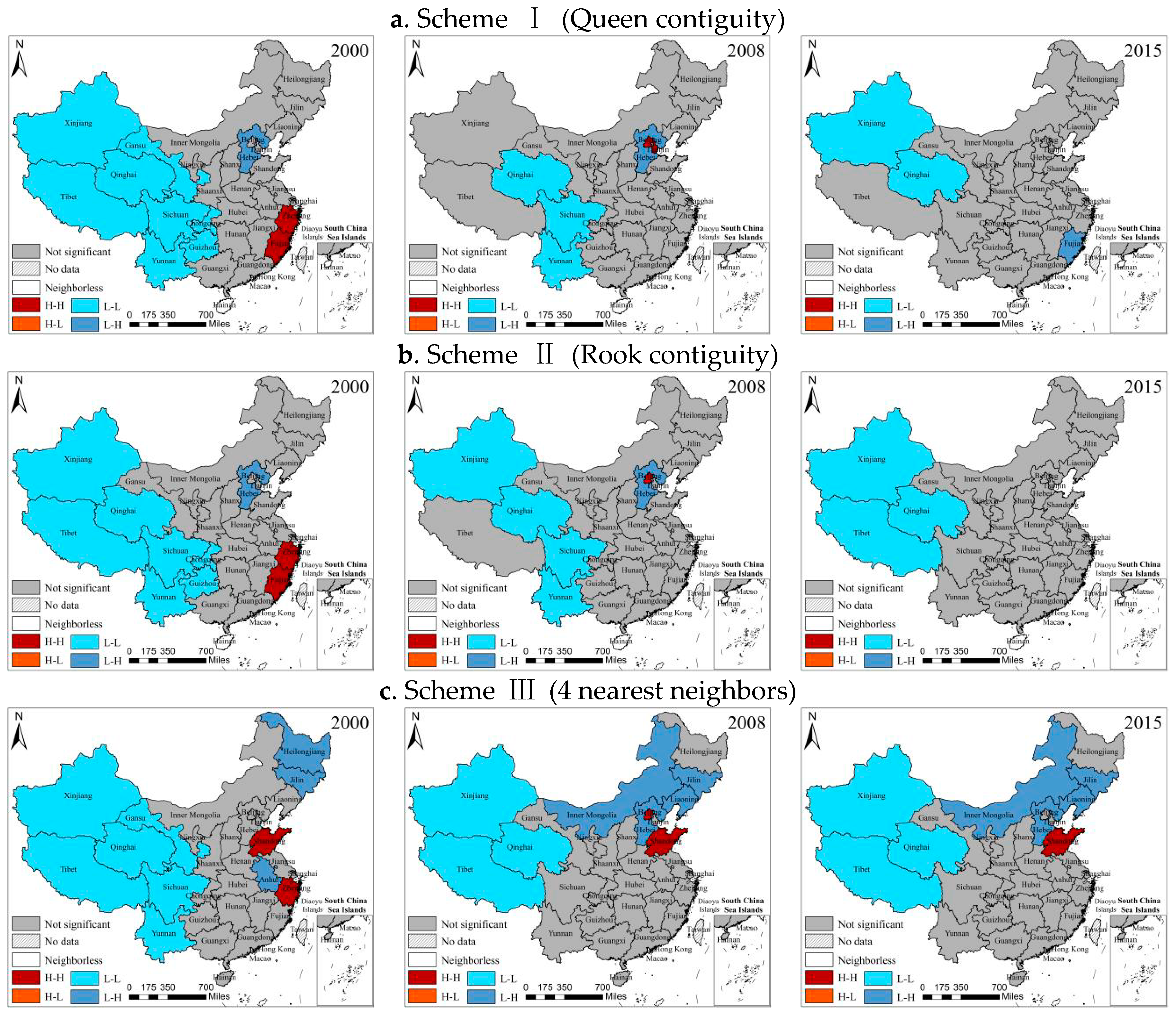
To further reveal the spatial distribution characteristics of the similar attribute values in specific regions, we assessed spatial dependence among the 31 provinces by analyzing the local indicators of spatial association based on Moran scatter plots and the local spatial autocorrelation index (LMI), taking 2000, 2008, and 2015 as an example, and at the 0.05 significance level, the local spatial autocorrelation cluster of eco-efficiency in mainland China is shown in Figure 1.

Comparison of Scheme I and Scheme II (Figure 1a,b) shows that except for Scheme II, which failed to identify Gansu as a significant low-low clustering area in 2000, the two schemes identified significant low-high clustering and high-high clustering basically the same. Compared with scheme I, the identified low-low clustering areas based on Scheme II increased Xinjiang but failed to identify Tianjin as a significant high-high clustering area in 2008. Both schemes (I and II) detected Xinjiang and Qinghai as significant low-low clustering areas, where Scheme II identified significant low-high clustering characteristics of Tibet but failed to detect other significant clustering types.

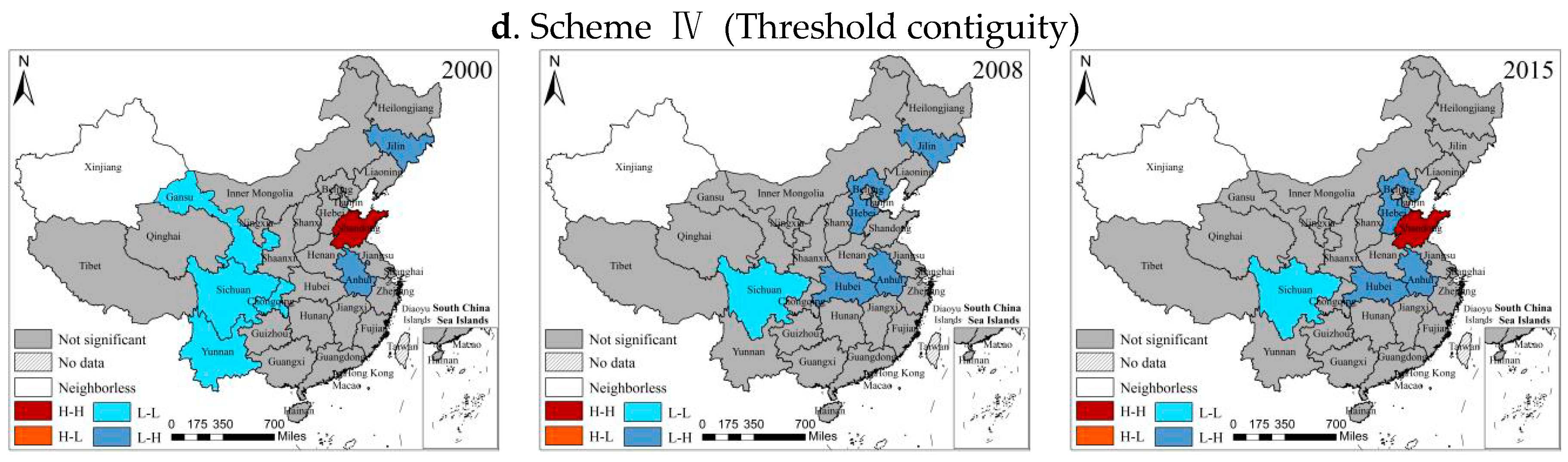
Figure 1c,d reflect that the two schemes identified significant low-low clustering areas (Gansu, Sichuan, Yunnan), significant high-high clustering areas (Shandong), and significant low-high clustering areas (Jilin, Anhui) and are more consistent, but compared with Scheme IV, Scheme III identified more significant areas in 2000. In 2008, although both schemes identified Jilin and Hebei as significant low-high clustering areas, Scheme III was more advantageous than Scheme I in identifying high-high clustering areas and low-low clustering areas. In 2015, both schemes identified Shandong and Hebei as significant high-high clustering areas and low-high clustering areas, respectively. However, Scheme III is still better than Scheme IV in terms of recognition capability.

The evaluation results of the above four schemes are mainly affected by factors, such as the size of the unit being assessed and the adjacency status. For example, in Scheme I and Scheme II, there are no direct neighbor relationships between Hainan and other provinces, which is difficult to identify effectively with two schemes.

The different value of K in Scheme III will lead to the randomness and uncertainty of the evaluation results. In Scheme IV, because the distance between the center of Xinjiang and the center of other areas exceeds the threshold distance, the Xinjiang area was judged neighborless, so it failed to identify the local spatial autocorrelation feature of the spatial unit. If the threshold distance is increased, it will inevitably affect the judgment of the number of neighbors in other provinces, resulting in not only random evaluation results, but there is uncertainty.

In addition, Scheme I and Scheme II have relatively good recognition results for low-low clustering areas, but both have poor recognition of low-high clustering areas. Scheme III and Scheme IV have a better recognition effect for low-high clustering areas. However, Scheme IV can easily reduce the scope of low-low clustering areas. However, the four schemes have poor ability to identify high-high agglomeration areas.

Overall, the first two schemes are more suitable for small-scale areas with relatively clear public edges or common points. The latter two solutions are suitable for large-scale space detection, but these two schemes are inevitably influenced by the subjective factors in the setting of threshold distance and the selection of K value, which leads to the limitation of evaluation results. Therefore, we will analyze it again based on the improved spatial weight scheme.

3.3. Analysis of Evaluation Results Based on Asymmetrical Spatial Weight Matrix

3.3.1. Global Spatial Autocorrelation Analysis of Eco-Efficiency in Mainland China Based on the EETI-Distance Reciprocal Principle

Through the analysis of the above evaluation results, we can see that the construction of spatial weight has a greater impact on the results of spatial autocorrelation analysis. Therefore, to further improve the reliability of the evaluation results, under the premise of fully considering the regional ecosystem service value and the difference in economic development level, the combined spatial weight scheme based on the EETI-distance reciprocal principle (Equation (10)) is used to test the GMI index and its significant level of eco-efficiency in 2000–2015, and the results are shown in

Table 3. Local spatial autocorrelation index and its significance test of eco-efficiency in mainland China based on asymmetrical spatial weight matrix.

Weight Scheme	Statistics	2000	2001	2002	2003	2004	2005	2006	2007
Scheme V (EETI-distance reciprocal)	GMI	0.108 ***	0.096 ***	0.091 ***	0.089 ***	0.044 **	0.083 ***	0.052 **	0.090 ***
	Z-value	3.639	3.340	3.198	3.162	1.989	2.998	2.205	3.185
	p-value	0.000	0.000	0.001	0.001	0.023	0.001	0.014	0.001
	Statistic	2008	2009	2010	2011	2012	2013	2014	2015
	GMI	0.085 ***	0.071 ***	0.074 ***	0.065 ***	0.061 ***	0.064 ***	0.060 ***	0.059 ***
	Z-value	3.045	2.678	2.778	2.543	2.439	2.504	2.418	2.381
	p-value	0.001	0.004	0.003	0.006	0.007	0.006	0.008	0.009

Note: * denotes 10% significance level, ** denotes 5% significance level, *** denotes 1% significance level. EETI: eco-economic transformation index; GMI: global Moran’s I.

.

As Table 3 shows, the GMI indices calculated based on Scheme V are positive, and the Z values are all greater than 1.96, indicating that the GMI indices passed the 5% significance test during the study period and presented a significant global positive correlation of eco-efficiency. From the perspective of the time series, the GMI index has risen during the four time periods of 2004–2005, 2006–2007, 2009–2010, and 2012–2013, indicating that the clustering effect of eco-efficiency is weakly increasing during this period, but the GMI index as a whole showed a declining tendency during the study period, illustrating that the clustering effect of eco-efficiency in mainland China tends to weaken with the passage of time. At the same time, the gradual decrease in the p-value and Z-value indicates that the global positive correlation is decreasing gradually; that is, the number of the significant high-high clustering areas or low-low clustering areas is decreasing gradually.

3.3.2. Local Spatial Autocorrelation Analysis of Eco-Efficiency in Mainland China Based on the EETI-Distance Reciprocal Principle

Combined with the Moran scatter chart and the LMI index, taking 2000, 2008, and 2015 as examples, and at the 5% significance level, the local spatial autocorrelation cluster of eco-efficiency in mainland China, which used the combined spatial weight scheme (Scheme V) based on the EETI-distance reciprocal principle, yields the results shown in Figure 2.

Figure 2 reveals that Scheme V failed to identify significant high-low and low-low clustering areas during the study period. The total number of positive spatial autocorrelation areas (high-high clustering) of eco-efficiency has been reduced from eleven to four. The concrete manifestation is that Inner Mongolia, Liaoning, Jiangsu, Fujian, Jiangxi, Zhejiang, and Hainan have exited from the high-high clustering areas. The results are consistent with the continued downward trend of the GMI indices, and its significance level is derived from Table 3.

In terms of geographical distribution, high-high clustering areas are mainly located in eastern China. Among these areas, the significance of Beijing, Tianjin, Shanghai, and Guangdong have remained unchanged during the study period, indicating that the capital conversion rate, resource utilization efficiency, and the ecological-economic transformation capacity are relatively high, and the cost of resource and environmental losses are relatively low. The industrial structure of the eastern provinces of China is relatively complete, thus forming significant high-high clustering areas with eco-efficiency.

The number of provinces showing low-high clustering areas increased from 10 in 2000 to 11 in 2015, among which Xinjiang, Tibet, Qinghai, Ningxia, and Guangxi provinces remained significant low-high clustering. On the whole, in addition to the eastern part of Hainan, the significant low-high clustering areas are located in the central and western regions of China.

4. Analysis of the Convergence of Eco-Efficiency in Mainland China

4.1. Convergence Model

Through the above spatial autocorrelation analysis of eco-efficiency in China, we can see that the spatial distribution of regional eco-efficiency is quite different. Whether the differences among regions will gradually decrease with time, and whether there is the same convergence pattern, all of these should be further analyzed. To this end, this paper has analyzed the convergence of China’s eco-efficiency to explore more deeply the regional differences in China’s eco-efficiency and its influencing factors. Since the eco-efficiency values obtained by Equation (1) are all relative efficiency values, convergence analysis cannot be performed. Therefore, we have analyzed the convergence of EETFPs in China and three major regions. Specific convergence methods include σ convergence, absolute β convergence, and conditional β convergence. According to Equation (11), σ convergence can be measured by the standard deviation of the EETFP in mainland China and three major regions [39]. A clear decline in the standard deviation over time would indicate that the EETFP gap among provinces has gradually been narrowing and that σ convergence exists. The measurement of absolute β convergence can be observed in Equation (12), which implies that the EETFP of all provinces converge to the same steady state if coefficient β is significantly negative. In addition, the measurement of conditional β convergence can be observed in Equation (13), which implies that the EETFP of provinces in different regions converges to their own steady states if coefficient β is negative [40].

σ convergence:

$$\sigma =\sqrt{\left[{\displaystyle \sum _{i=1}^n{\left(\ln Y_{i,t}-\frac{1}{n}{\displaystyle \sum _{i=1}^n\ln Y_{i,t}}\right)}^2}\right]/n}$$

(11)

absolute β convergence:

$$\frac{1}{T}=\ln \left(Y_{i,t+1}/Y_{t,t}\right)={\alpha }_1+{\beta }_1\ln Y_{i,t}+{\displaystyle \sum _{j=1}^J{\gamma }_j{x}_{i,t}^j}+{\epsilon }_{i,t}$$

(12)

conditional β convergence:

$$\frac{1}{T}\ln \left(Y_{i,t+T}/Y_{i,0}\right)={\alpha }_0+{\beta }_0\ln Y_{i,0}+{\epsilon }_{i,t}$$

(13)

where lnY_i,0 and lnY_i,t represent the EETFP logarithm of the eco-efficiency of the initial period and t^th period of the i^th region, respectively, and i = 1, 2, …, n represents the provinces. α₀ and α₁ are constants, ε_i,t is the stochastic error, and T represents the study period. $x_{i,t}^j$ is the j^th influencing factor of the i^th province in period t.

4.2. σ Convergence

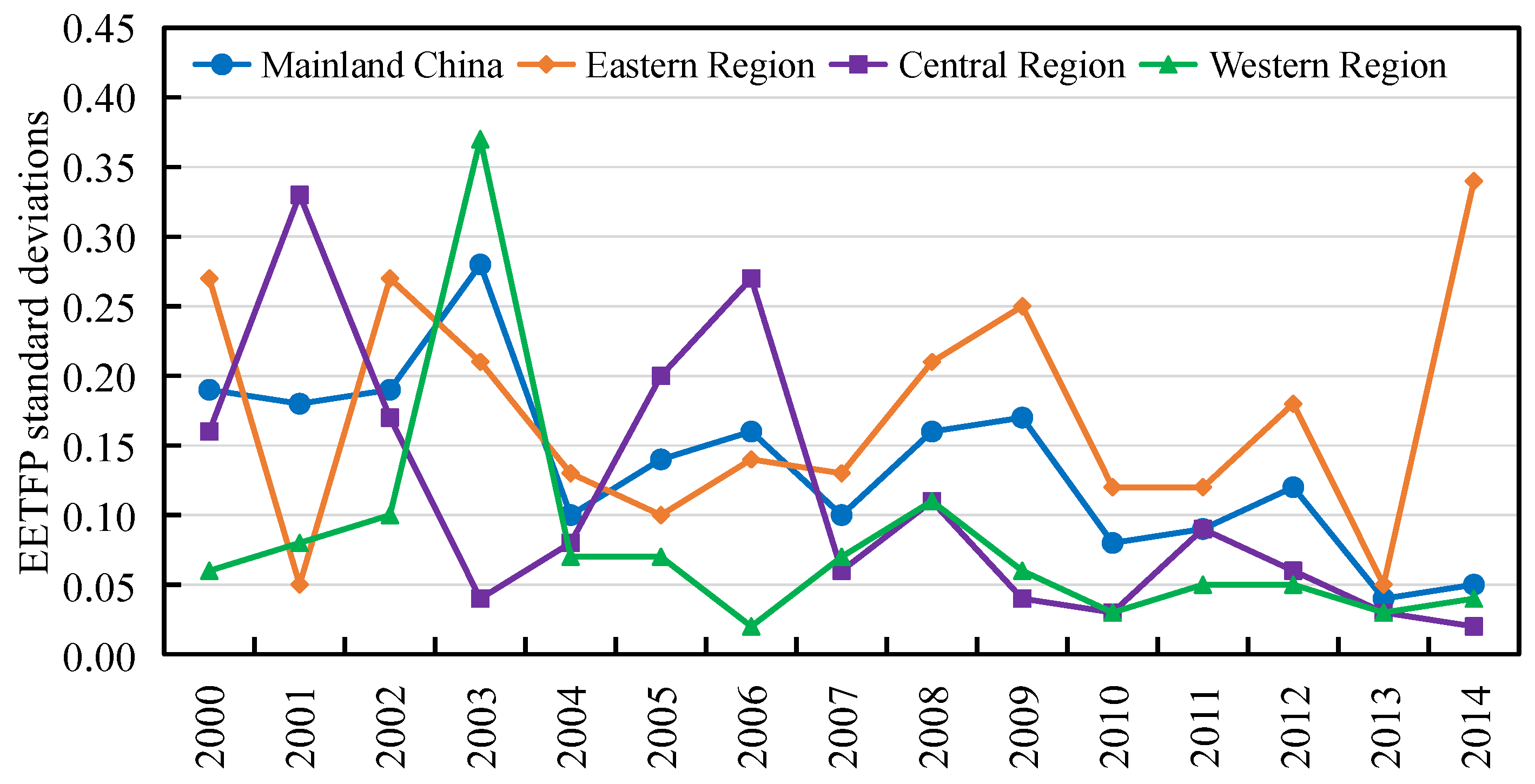
According to Equation (11), the EETFP of China and three major regions is calculated. These regions are the eastern region (Beijing, Tianjin, Hebei, Liaoning, Jiangsu, Shanghai, Zhejiang, Fujian, Shandong, Guangdong, Hainan), central region (Shanxi, Jilin, Heilongjiang, Anhui, Jiangxi, Henan, Hubei, Hunan), and western region (Inner Mongolia, Guangxi, Chongqing, Sichuan, Guizhou, Yunnan, Tibet, Shaanxi, Gansu, Qinghai, Ningxia, Xinjiang). The σ convergence of the EETFP in mainland China and three major regions is shown in Figure 3.

Figure 3 shows that during the study period, the eastern value of the standard deviation of EETFP is 0.17. However, the average value of mainland China and the central region is 0.14, 0.11, while the mean of the western region is the smallest, 0.08. In addition to the eastern region, the EETFP in remaining regions shows a trend of decreasing fluctuation during the study period, which indicates that there is σ convergence in mainland China, central region, and western region, indicating that the gaps gradually decrease in the study. However, there is no σ convergence in the eastern region, indicating that the gaps do not disappear in the study period.

4.3. Absolute β Convergence

According to Equation (12), the results of absolute β convergence are shown in

Table 4. Absolute β convergence test of EETFP in mainland China and three major regions.

Statistics	Regions
	Mainland China	Eastern Region	Central Region	Western Region
Constant	0.028	0.012	0.087	0.005
	(0.810)	(0.714)	(1.201)	0.223
β	−0.150 ***	−0.219 **	−0.102	−0.026
	(−3.017)	(−2.562)	(−1.093)	(−0.322)
R2	0.098	0.360	0.0700	0.098

Note: *, **, and *** represent the significance level of 10%, 5%, and 1%, respectively. The values in the parentheses refer to t-values.

. Table 3 shows that the results support absolute β convergence for all regions during the study period, and the mainland China and eastern region have significant negative β values, indicating that there is a trend of absolute β convergence of EETFP in mainland China and the eastern region, indicating that the eco-efficiency of the growth rate of China will tend to a common level, and the gaps in the eastern region will gradually decrease in the future.

Although the β in the central and western regions was negative, it did not pass the 5% significance level test, indicating that there was no absolute β convergence of EETFP in the central and western regions, which also reflected the differences in production management and technical level in the central and western provinces.

Therefore, the differences in EETFP between mainland China and the eastern regions would gradually disappear over time, while the differences in EETFP between the central and western regions would continue to exist. At the same time, as shown in Figure 3, there is σ convergence in mainland China, indicating that there is club convergence in China.

4.4. Conditional β Convergence

Since the absolute β convergence model uses the initial level of EETFP as the only factor that determines its convergence, there are in fact many factors that actually affect the EETFP convergence. We select the per capita ecosystem service value (PESV), ecological-economic transformation index (EETI), and resource and environmental cost of unit GDP (RECGp) to reflect ecological resource endowments; per capita GDP (PGDP) and foreign direct investment (FDI) to reflect regional economic development level; research and development input (R&D) to reflect the level of science and technology; proportion of tertiary industry (PTI) to reflect social development status. Taking these seven indicators as the conditional variables, according to Equation (13), the results of conditional β convergence are shown in

Table 5. Conditional β convergence test of EETFP in mainland China and three major regions.

Statistics	Regions
	Mainland China	Eastern Region	Central Region	Western Region
Constant	0.068	0.025	0.265 ***	−0.127
	(0.643)	(0.071)	(2.943)	(−1.242)
β	−0.182 ***	−0.269 ***	−0.314 ***	−0.067
	(−3.692)	(−3.272)	(−3.101)	(−0.824)
PESV	1.04 × 10−7	−4.77 × 10−5	−0.624 ***	3.60 × 10−7
	(0.221)	(−0.734)	(−3.322)	(1.357)
PGDP	3.64 × 10−6 ***	1.25 × 10−5 ***	0.076	1.14 × 10−6
	(3.29)	(3.195)	(0.367)	(0.892)
FDI	6.25 × 10−5	2.72 × 10−5	0.064	2.19 × 10−4
	(1.613)	(0.483)	(1.638)	(1.156)
R&D	−2.86 × 10−4 ***	−4.59 × 10−4 ***	0.443 ***	−4.18 × 10−4
	(−2.872)	(−2.823)	(7.052)	(−1.116)
PTI	−0.202	−0.287	−0.811	0.225
	(−0.796)	(−0.425)	(−1.416)	(0.876)
EETI	0.002	0.006 ***	0.080 ***	0.005
	(1.923)	(2.654)	(3.854)	(0.512)
RECGp	−0.001	0.820	−1.218 ***	−0.001
	(0.647)	(1.623)	(−3.547)	(−0.663)
R2	0.735	0.716	0.927	0.348

Note: *, ** and *** represent the significance level of 10%, 5% and 1%, respectively. The values in the parentheses refer to t-values. PESV: per capita ecosystem service value; PGDP: per capita GDP; FDI: foreign direct investment; R&D: research and development input; PTI: proportion of tertiary industry; EETI: ecological-economic transformation index; RECGp: resource and environmental cost of unit GDP.

.

Table 5 shows that the convergence coefficient β of each region is significantly negative except for the western regions. Therefore, we can conclude that there are conditional β convergence characteristics in the national, eastern, and central regions, indicating that the EETFP values in these regions will converge to their own steady level states over time.

From the perspective of various influencing factors, per capita ecosystem service value and unit GDP resource environment cost consumption are significantly negative in the central region. PGDP shows significant positive characteristics in mainland China and the eastern region, and R&D investment is significantly negative in mainland China and the eastern region, but it is significantly positive in the central region. EETI is significantly positive in the eastern and central regions. But it should be noted that although there is significant conditional β convergence in the central region, there is no absolute β convergence, indicating that the central provinces and regions have not converged to a common EETFP, but due to the differences in ecosystem service value endowments, industrial structure, science and technology level, and production management among provinces and regions in the region, each province and region tends to its own stable state.

5. Conclusions and Suggestions

In this paper, we applied the SBM model to measure the eco-efficiency of 31 provinces in China during 2000–2015 and analyzed the interprovincial spatial patterns of eco-efficiency based on the symmetry spatial weight scheme. Then, we introduced a new combined spatial weight scheme based on the EETI-distance reciprocal principle, which was used to analyze the global spatial autocorrelation of eco-efficiency. For further analysis, we used convergence models to explore the convergence of EETFP of China and three major regions. The results showed that the eco-efficiency had significant global Moran’s I value (at the 0.05 significance level), but the clustering effect of eco-efficiency in mainland China tended to weaken with the passage of time, and the high-high clustering regions were mainly located in eastern China while low-high clustering regions were mainly in the central and western regions of China according to province-scale LISA analysis. We also found that China expressed the club convergence and there was no σ convergence in the eastern region, and there was no absolute β convergence in the central and western regions. From the perspective of conditional β convergence, all regions except for the western region showed conditional β convergence.

Evidence from the empirical analysis revealed that the central and western regions should further accelerate the adjustment of industrial structure and change the mode of economic development. Meanwhile, relying on their own high values of ecosystem services, they should speed up the linkage of funds and technology costs with the eastern provinces and improve the ecological-economic transformation capability, thereby promoting the evolution of the regional economy, social development, resources, and the environment to a dynamic balance. According to the analysis of convergence, we also found that the central regions should reduce the utilization of regional ecosystem service values and the consumption of unit GDP resources and environmental costs, improve the utilization rate of resources and promote the eco-efficiency. The country still needs to take regional economic development as the first priority, especially in the eastern regions, and should rely on its advantages in capital, science and technology, and production management to accelerate regional economic and social development to further improve regional eco-efficiency. Increasing the utilization rate of R&D investment in science and technology in the country and in the eastern regions would have a significant role in promoting regional eco-efficiency. But the central regions should attach great importance to scientific and technological progress, and scientific research input has a significant driving role in promoting the regional eco-efficiency. The eastern and central regions should improve the ecological-economic transformation capacity which is conducive to increase regional EETFP. The central regions should especially pay more attention to the transformation of economic efficiency while reducing the development and utilization of ecosystem service values.

The research results provide a significant reference for regional ecological management and sustainable regional transformation in China. To improve the eco-efficiency and regional economic development quality, it is important to transform the traditional extensive development model which relies on high consumption, high emissions, and high pollution, and promote a low-carbon, green, and sustainable urban transformation. There is a need to improve the intensive degree of resource utilization, optimize the spatial distribution of resource allocation, develop more advanced energy-saving and water-saving technologies, and the results can be used by decision-makers for sustainable planning and development.

References

- Schaltegger, S.; Sturm, A. Ökologische Rationalität: Ansatzpunkte zur Ausgestaltung von ökologieorientierten Managementinstrumenten. Die Unternehmung 1990, 44, 273–290. [Google Scholar]
- World Business Council for Sustainable Development (WBCSD). Eco-Efficient Leadership for Improved Economic and Environmental Performance; WBCSD: Conches-Geneva, Switzerland, 1996. [Google Scholar]
- Organisation for Economic Co-operation and Development. Eco-Efficiency; OECD: Geneva, Switzerland, 1998; pp. 7–11. [Google Scholar]
- Saling, P.; Kicherer, A.; Dittrich-Krämer, B.; Wittlinger, R.; Zombik, W.; Schmidt, I.; Schrott, W.; Schmidt, S. Eco-efficiency Analysis by BASF: The Method. Int. J. Life Cycle Assess. 2002, 7, 203–218. [Google Scholar] [CrossRef]
- United Nations Conference on Trade and Development (UNCTD). Integrating Environmental and Financial Performance at the Enterprise Level: A Methodology for Standardizing Eco-Efficiency Indicators; United Nations Publication: New York, NY, USA, 2003; pp. 29–30. [Google Scholar]
- An, V.; Spirinckx, C.; Geerken, T. Life cycle assessment and eco-efficiency analysis of drinking cups used at public events. Int. J. Life Cycle Assess. 2010, 15, 221–230. [Google Scholar]
- Van Caneghem, J.; Block, C.; Cramm, P.; Mortier, R.; Vandecasteele, C. Improving eco-efficiency in the steel industry: The ArcelorMittal Gent case. J. Clean. Prod. 2010, 18, 807–814. [Google Scholar] [CrossRef]
- Michelsen, O.; Fet, A.M.; Dahlsrud, A. Eco-efficiency in extended supply chains: A case study of furniture production. J. Environ. Manag. 2006, 79, 290–297. [Google Scholar] [CrossRef]
- Neto, J.Q.F.; Walther, G.; Bloemhof, J.; van Nunen, J.A.E.E.; Spengler, T. A Methodology for Assessing Eco-Efficiency in Logistics Networks. Eur. J. Oper. Res. 2009, 193, 670–682. [Google Scholar] [CrossRef]
- Egilmez, G.; Gumus, S.; Kucukvar, M.; Tatari, O. A Fuzzy Data Envelopment Analysis Framework for Dealing with Uncertainty Impacts of Input-Output Life Cycle Assessment Models on Eco-efficiency Assessment. J. Clean. Prod. 2016, 129, 622–636. [Google Scholar] [CrossRef]
- Martín-Gamboa, M.; Iribarren, D.; Dufour, J. Environmental impact efficiency of natural gas combined cycle power plants: A combined life cycle assessment and dynamic data envelopment analysis approach. Sci. Total Environ. 2018, 615, 29–37. [Google Scholar] [CrossRef] [PubMed]
- Lahouel, B.B. Eco-efficiency analysis of French firms: A data envelopment analysis approach. Environ. Econ. Policy Stud. 2016, 18, 395–416. [Google Scholar] [CrossRef]
- Wursthorn, S.; Poganietz, W.R.; Schebek, L. Economic–environmental monitoring indicators for European countries: A disaggregated sector-based approach for monitoring eco-efficiency. Ecol. Econ. 2011, 70, 487–496. [Google Scholar] [CrossRef]
- Van Middelaar, C.E.; Berentsen, P.B.M.; Dolman, M.A.; de Boer, I.J.M. Eco-efficiency in the production chain of Dutch semi-hard cheese. Livest. Sci. 2011, 139, 91–99. [Google Scholar] [CrossRef]
- Maia, R.; Silva, C.; Costa, E. Eco-efficiency assessment in the agricultural sector: The Monte Novo irrigation perimeter, Portugal. J. Clean. Prod. 2016, 138, 217–228. [Google Scholar] [CrossRef]
- Ullah, A.; Perret, S.R.; Gheewala, S.H.; Soni, P. Eco-efficiency of cotton-cropping systems in Pakistan: An integrated approach of life cycle assessment and data envelopment analysis. J. Clean. Prod. 2016, 134, 623–632. [Google Scholar] [CrossRef]
- Chen, L.M.; Wang, W.P.; Wang, B. Economic Efficiency, Environmental Efficiency and Eco-efficiency of the So-called Two Vertical and Three Horizontal Urbanization Areas: Empirical Analysis Based on HDDF and Co-Plot Method. China Soft Sci. 2015, 2, 96–109. [Google Scholar]
- Peng, H.; Zhang, J.H.; Lu, L.; Yan, B.J.; Xiao, X.; Han, Y. Eco-efficiency and its determinants at a tourism destination: A case study of Huangshan National Park, China. Tour. Manag. 2017, 60, 201–211. [Google Scholar] [CrossRef]
- Li, Z.; Ouyang, X.L.; Du, K.R.; Zhao, Y. Does government transparency contribute to improved eco-efficiency performance? An empirical study of 262 cities in China. Energy Policy 2017, 110, 79–89. [Google Scholar] [CrossRef]
- Wang, S.J.; Ma, Y.Y. Influencing factors and regional discrepancies of the efficiency of carbon dioxide emissions in Jiangsu, China. Ecol. Indic. 2018, 90, 460–468. [Google Scholar] [CrossRef]
- Ren, S.G.; Li, X.L.; Yuan, B.L.; Li, D.Y.; Chen, X.H. The effects of three types of environmental regulation on eco-efficiency: A cross-region analysis in China. J. Clean. Prod. 2018, 173, 245–255. [Google Scholar] [CrossRef]
- Zhang, J.X.; Liu, Y.M.; Chang, Y.; Zhang, L.X. Industrial eco-efficiency in China: A provincial quantification using three-stage data envelopment analysis. J. Clean. Prod. 2017, 143, 238–249. [Google Scholar] [CrossRef]
- Huang, J.H.; Xia, J.J.; Yu, Y.T.; Zhang, N. Composite eco-efficiency indicators for China based on data envelopment analysis. Ecol. Indic. 2018, 85, 674–697. [Google Scholar] [CrossRef]
- Li, J.; Deng, C.X.; Zhang, S.T. The evaluation and dynamic analysis on regional eco-efficiency based on Non-parametric Distance Function. J. Arid Land Resour. Environ. 2015, 29, 19–23. [Google Scholar]
- Cheng, J.H.; Sun, Q.; Guo, M.J.; Xu, W.Y. Research on Regional Disparity and Dynamic Evolution of Eco-efficiency in China. China Popul. Resour. Environ. 2012, 24, 47–57. [Google Scholar]
- Bai, Y.P.; Deng, X.Z.; Jiang, S.J.; Zhang, Q.; Wang, Z. Exploring the relationship between urbanization and urban eco-efficiency: Evidence from prefecture-level cities in China. J. Clean. Prod. 2018, 195, 1487–1496. [Google Scholar] [CrossRef]
- Charnes, A.; Cooper, W.W.; Rhodes, E. Measuring the efficiency of decision making units. Eur. J. Oper. Res. 1978, 2, 429–444. [Google Scholar] [CrossRef]
- Tone, K. A slacks-based measure of super-efficiency in data envelopment analysis. Eur. J. Oper. Res. 2002, 143, 32–41. [Google Scholar] [CrossRef] [Green Version]
- Tone, K. A slacks-based measure of efficiency in data envelopment analysis. Eur. J. Oper. Res. 2001, 130, 498–509. [Google Scholar] [CrossRef] [Green Version]
- Färe, R.; Grosskopf, S.; Noh, D.W.; Weber, W. Characteristics of a polluting technology: Theory and practice. J. Econom. 2005, 126, 469–492. [Google Scholar] [CrossRef]
- Wang, H.F.; Shi, Y.S.; Ying, C.Y. Land use efficiencies and their changes of Shanghai’s development zones employing DEA model and Malmquist productivity index. Geogr. Res. 2014, 33, 1636–1646. [Google Scholar]
- Sawada, M. Global Spatial Autocorrelation Indices-Moran’s I, Geary’s C and the General Cross-Product Statistic; Laboratory for Paleoclimatology and Climatology at the University of Ottawa: Ottawa, ON, Canada, 2004. [Google Scholar]
- Moran, P.A.P. The statistical analysis of the Canadian Lynx cycle. Aust. J. Zool. 1953, 1, 291–298. [Google Scholar] [CrossRef]
- Parent, O.; Lesage, J.P. Using the variance structure of the conditional autoregressive spatial specification to model knowledge spillovers. J. Appl. Econom. 2008, 23, 235–256. [Google Scholar] [CrossRef]
- Dey-Chowdhury, S. Methods explained: Perpetual Inventory Method (PIM). Econ. Labour Mark. Rev. 2008, 2, 48–52. [Google Scholar] [CrossRef] [Green Version]
- Shan, H.J. Re-estimating the capital stock of China: 1952–2006. J. Quant. Tech. Econ. 2008, 25, 17–31. [Google Scholar]
- Wu, J.D.; Li, N.; Shi, P. Benchmark wealth capital stock estimations across China’s 344 prefectures: 1978 to 2012. China Econ. Rev. 2014, 31, 288–302. [Google Scholar] [CrossRef]
- Berlemann, M.; Wesselhöft, J.E. Estimating Aggregate Capital Stocks Using the Perpetual Inventory Method. Rev. Econ. 2014, 65, 1–34. [Google Scholar] [CrossRef]
- Quah, D. Galton’s Fallacy and Tests of the Convergence Hypothesis. Scand. J. Econ. 1993, 95, 427–443. [Google Scholar] [CrossRef]
- Sala-I-Martin, X.X. Regional cohesion: Evidence and theories of regional growth and convergence. Eur. Econ. Rev. 1994, 40, 1325–1352. [Google Scholar] [CrossRef]
Figure 1.
Local spatial autocorrelation cluster of eco-efficiency in mainland China based on scheme I to scheme IV.
Figure 2.
Local spatial autocorrelation cluster of eco-efficiency in mainland China based on scheme V.
Figure 3.
The standard deviation trends of EETFP in mainland China and three major regions.