Application of the Operational Research Method to Determine the Optimum Transport Collection Cycle of Municipal Waste in a Predesignated Urban Area

Abstract

This paper deals with waste management. The aim is to find out whether the number of municipal mixed waste bins can be reduced due to the impact of waste separation and to determine the optimum municipal waste collection cycle within a predesignated area with an existing urban road network. The number of mixed waste bins depends on two factors—household waste volume and household waste composition. Both of these factors have a significant impact on the number of mixed waste bins required, with household waste composition being of particular importance when it comes to calculating the potential reduction in the number of mixed waste bins required due to waste separation. The calculations for the weight and volume of mixed household waste per person and the composition (types) thereof are presented accordingly. The results reveal which types of waste are the most useful in minimising the number of mixed waste bins by up to 30–50%. To determine the optimum waste collection cycle within the predesignated area with a real urban road network, the Nearest Neighbour Search method was applied. In the discussion, the focus is on whether other methods, including the Two-Phase Heuristic approach and the Bellman-Ford Algorithm, could be applied to solve the problem, whereby parameters such as application time and the capacity of the waste collection vehicle are compared.

1. Introduction

Waste management involves, among other things, waste classification, waste prevention, waste collection and transportation, waste handling and disposal, aftercare of the places where the waste is permanently stored, and environmental impact. Waste management is a dynamically evolving sector within the national economy. Industrially and economically advanced countries only began to seriously deal with the issue of waste management in the 1980s. Country-specific waste management legislation is primarily focused on waste prevention. This is crucial in regard to the state of the environment and the use of non-renewable resources. The support of the State for cleaner waste production was one of the key points [1,2].

Setting out the objectives and identifying the specific activities relating to waste management are essential preconditions for choosing suitable logistics processes and waste management instruments. In order to put forward waste management solutions, it is appropriate to carry out a detailed analysis similar to the one presented here. Such an analysis may include alternative situations, but only within the context of the need to separate the recommended logistics tools for the individual alternatives [2,3,4]. Within the context of waste management, and from the point of view of the sustainable development of environment friendly policies [5], the issues of collection and sorting are important contributory factors [1].

The efficient distribution of waste bins and the cycle of collection represent other aspects of high-quality waste management [6]. The aim of this paper is, therefore, to quantify the reduction in the number of municipal mixed waste bins required due to the impact of waste separation and to determine the optimum waste collection cycle in a predesignated area, which is located in a selected part of the South Bohemia region, on the basis of an existing urban road network.

The current situation in terms of waste collection cycle does not take into consideration the potential and alignment of a road communication network. Given those circumstances, this inappropriate state needed to be streamlined appropriately. The objective of the paper is also to propose an appropriate waste collection cycle when using the selected operational research method. Performing the preliminary relevant methods analysis, the Nearest Neighbour Search Method is chosen as the most suitable method for the purpose of this research study [7].

In regard to discussion of achieved results, comparison of this method with other methods, which may be potentially applicable for the given issue, are specified. Particularly, Distributing or Two-Phase Heuristic method and Bellman-Ford Algorithm are described in the context of their application within the research topic [7].

The waste management issue is addressed in a number of publications [1,2,3,4,5,6,7,8,9,10,11,12,13,14,15,16,17,18]. Some publications [1,2,3,4,5] focus on the impact of waste management on the environment, whilst others [6,8] focus on waste management in certain industrial sectors. For example, a previous study [5] focuses on eco-waste management through the possible use of cellulose waste combined with municipal waste to produce new materials, another study [6] focuses on waste management in hotel operations, another [8] focuses on the decision-making behaviour of contractors and government ministries in the field of construction, and yet another study [19] on innovative solutions for municipal waste management.

The sustainable management of municipal waste is dealt with in previous studies [20,21]. In another study [22], a multi-criteria sustainability assessment of waste management in the UK is the focus. In yet another study [23], the sustainability of municipal waste landfilling and composting in the north of Iran is addressed. An assessment of the financial sustainability of waste management on the basis of various factors is made in a previous study [24]. The authors conclude that the most important aspect of the financial sustainability of waste management is the assessment of the contextual factors. The analysis focuses on problems in Italian municipalities. The article goes on to point out the importance of waste separation.

This paper, on the basis of a case study, also explores the impact of waste separation on overall waste management. As part of the case study, calculations are presented in regard to the need for municipal waste bins under two conditions—with and without waste separation. In addition, calculations are presented that show which types of separated waste produce the greatest reduction in the number of required municipal waste bins. The results are very close to the required 50% recovery rate referred to in a previous work [25]. In this article, the author points to the fact that the 50% recovery rate has yet to be achieved in Geneva. In another study [26], it is suggested that the Automatic Sorting Technology Methodology should be used to support electronic waste classification, with a holistic approach to addressing the issue. The methodology is applicable not only to electronic waste management. In a previous work [27], Pasotti addresses the waste crisis economically linked to the slow transition to waste treatment and recycling in southern Italy in 2010. In previous studies [28,29], the authors deal with waste sorting and recycling.

The lifecycle and handling of municipal waste are dealt with in other works [30,31,32,33,34,35]. Case studies related to the assessment of the waste management lifecycle are presented in previous studies [32,33,35]. For example, one study [32] focuses on the assessment of the sustainability of China’s waste management system, while another [33] on the lifecycle of plastics in India, and a third [35] on general municipal solid waste in Iran. The problems regarding waste management modelling are dealt with in other studies [7,36,37]. In this paper, the waste collection cycle is addressed within a particular area on the basis of the application of the Nearest Neighbour Search Method. This method is dealt with in previous works [7,38,39,40,41,42,43,44,45,46,47,48,49].

Even though some authors describe the adoption of the Nearest Neighbour Search heuristic to determine the optimum waste collection [50], as far as we are aware, there has not yet been any comprehensive methodology developed when taking into consideration the necessary number of municipal mixed waste bins, as well as the optimum waste collection cycle in a given transport territory. This makes this article unique. It was decided to implement this technique given the circumstances that the waste management, particularly determining the optimum frequency of the waste collection cycle, can be deemed as the issues identified to find the route with which to cover all points of interest. Precisely, the Nearest Neighbour Search heuristic fully comply with this set of aspects.

Several methods, e.g., the Bellman-Ford Algorithm, the Two-Phase Heuristic approach, or the Dijsktra algorithm, can also be applied to the issue of optimising the municipal waste collection cycle, which are discussed in previous works [51,52,53,54,55,56].

The transportation of municipal waste includes both the transport of the waste from the point it is generated (e.g., households) to the collection point (e.g., waste container site) and the transport from the collection point to the place of final disposal [57,58]. Generally speaking, the transportation of municipal waste can be classified according to [7]:

• transport distance; or
• means of transport used.

In regard to the transport distance among the centres of waste generation and disposal sites [58,59], the waste transportation can be conducted as a single-phase, two-phase, or multiphase process. In the Czech Republic, the transportation is predominantly single-phase. However, both two-phase and multiphase transportation are starting to develop slowly (e.g., MSTS system—Multi Service Transport System) [60].

In regard to the means of transport used, transportation by road is considered the most common type of solid municipal waste transportation [61]. In foreign countries, transportation by ship or rail is only used where longer distances (more than 250 km) need to be covered [57]. Where short distances (less than 250 km) are involved, it is possible to use road transport, air, or water piping systems [59].

Municipal waste transfer stations, as well as municipal waste container systems (as concepts included within the municipal waste transportation issues), are described in several scientific publications [57,59,62,63].

Waste collection in regard to standardised waste collection bins (containers) is carried out at specified regular intervals (Act No. 100/2001 Coll.) [64].

Sites intended for waste collection bins (containers) and facilities include [62,63]:

• waste collection container stations;
• waste collection points;
• facilities or sites designated for the storage of residual municipal waste.

2. Methods for Deployment of Municipal Solid Waste Bins

The deployment of waste bins is governed by two principles, namely adequate accessibility to services and adequate capacity within the waste collection system. Both principles are equally important in terms of establishing an appropriate and well-functioning waste collection system.

2.1. Waste Production Potential

The main criterion determining the qualitative and quantitative characteristics of municipal waste is the way in which apartments are heated. Within this context, it can be said that the Czech Republic has two different types of municipal waste. This division is based on the fact that the composition of municipal waste in built-up areas, in which municipal heating is provided to apartments (apartment blocks), is different to that in areas with family houses, in which local heating sources are used, i.e., predominantly solid fuel.

Research in the last few decades distinguishes between three types of built-up areas based on the prevailing types of buildings:

• housing development
• mixed-use development
• rural housing

A housing development is a built-up area with apartment blocks that utilise a centralised heat supply system and where there is no opportunity to utilise waste for heat generation. The share of premises for businesses and service providers is insignificant.

A mixed-use development is a built-up area with both apartment blocks (mostly in city centres) with centralised heat supply and apartments with local gas or electric heating. There are only a negligible number of apartments with solid fuel heating, while the share of premises for businesses and service providers is significant.

Rural housing consists of family houses with mostly local solid fuel heating. This means the options exist to incinerate household waste in home furnaces, to compost biodegradable waste, or to use part of the waste as feed. The share of premises for businesses and service providers is insignificant.

Table 1. Volume of household waste.

Type of Built-up Area	Volume of Waste
	kg/inhab./Week			kg/inhab./Year
	Average	Maximum	Minimum	Average
Housing development	3.4	3.9	2.5	179
Mixed-use development	3.6	4.2	3.2	189
Rural housing *)	5.9	8.5	2.8	308

Note: *) with mostly solid fuel heating. Source: Authors.

shows the volumes of household waste produced according to the type of built-up area.

As part of the analysis, a more detailed breakdown of the specific components of household waste was sought in order to determine its potential utilisation. The components were: paper (paperboard, cardboard, mixed-material packaging, other types of packaging, printed matter, other types of paper); plastics (foils, plastic bottles, other types of plastics); glass (glass packaging—clear, amber, or green, returnable glass packaging, other); metals (iron, aluminium, others). The results are presented in

Table 2. Composition of household waste (by % weight).

Components	Household Waste—Share of Individual Components (by % Weight), Average Values
	Housing Development	Mixed-Use Development	Rural Housing *)
Paper, paperboard	25.7	24.9	7.8
Plastics	16.8	19.0	9.7
Glass	11.2	8.5	4.9
Metals	1.7	2.1	2.6
Organic waste	15.6	19.6	11.7
Fabrics	4.5	3.7	2.3
Mineral wastes	2.2	0.5	6.8
Hazardous waste	0.5	0.5	0.3
Combustible waste	10.6	11.1	9.4
Waste EEE	0.6	0.5	0.3
Fraction 20–40 mm	5.0	4.2	4.9
Fraction 8–20 mm	2.8	3.2	7.8
Fraction under 8 mm	2.8	2.2	31.5
In total	100.0	100.0	100.0

Note: *) with mostly solid fuel heating. Source: Authors.

below.

The above shows that in terms of the composition of household waste, there are no big differences between housing developments and mixed-use developments. It is for this reason that in subsequent sections, these are referred to as one, namely housing developments.

2.2. Process for Determining the Number of Mixed Waste Bins

Determining what the adequate number of mixed waste bins per household is must be based on the worst-case scenario in terms of waste production and its collection. Waste production varies seasonally, with several peaks throughout the year. A rule of thumb used by most waste collection companies is that the average volume of waste produced per person per day is 5 L.

In terms of family homes, one waste bin (110–240 L) is usually allocated per household in order to guarantee sufficient capacity for effective and appropriate waste collection. When determining the number of waste bins for housing developments, the higher number of households and the associated higher waste production levels must be taken into consideration. Our analysis of the composition of municipal waste focused, inter alia, on the weight (bulk density) of mixed waste from households, but only after it was unloaded from waste collection vehicles. The average values for bulk density are presented in

Table 3. Weight (bulk density) of mixed waste from households (kg·m⁻³).

Type	Weight (Bulk Density) of Mixed Waste from Households
	(kg·m−3)
	Average	Maximum	Minimum
Housing development	266	232	183
Mixed-use development	292	351	207
Rural housing *)	476	494	211

Note: *) mostly solid fuel heating. Source: Authors.

.

The weights of the individual components in the mixed waste bins were determined on the basis of measurements carried out by waste management companies. The values were calculated based on the following assumed composition (see

Table 4. Weight of components in mixed waste from households.

Component	Weight (kg·m−3)
Paper, paperboard	100
Plastics	25
Glass	350
Metals	4000
Organic waste	500
Fabric	200
Mineral waste	2500
Hazardous waste	2000
Combustible waste	500
Fine fraction	1000

Source: authors.

):

On the basis of the share of the individual components in the mixed waste of households, it is possible to calculate the volumes of the individual components accordingly (see

Table 5. Volume of individual components in 1 kg of mixed waste.

Components	L·kg−1
Paper, paperboard	2.57
Plastics	6.72
Glass	0.32
Metals	0.004
Organic waste	0.312
Fabric	0.225
Mineral waste	0.009
Hazardous waste	0.006
Combustible waste	0.212
Fine fraction	0.106
In total	10.484

Source: Authors.

). By summing them up, it is possible to calculate the weight of mixed waste without waste separation in housing developments.

Additional calculations based on the waste production per person per day, as well as the weight of the individual components (see

Table 6. Amount of mixed waste without waste separation.

Mixed Waste Component	Average Production		Volume
	kg/Day	kg/Week	L/Day	L/Week
Paper, paperboard	0.126	0.882	1.26	8.82
Plastics	0.082	0.574	3.28	22.96
Glass	0.055	0.385	0.157	1.1
Metals	0.008	0.056	0.002	0.014
Organic waste	0.077	0.539	0.154	1.078
Fabric	0.022	0.154	0.11	0.77
Mineral wastes	0.011	0.077	0.004	0.031
Hazardous waste	0.003	0.021	0.002	0.011
Combustible waste	0.052	0.364	0.104	0.728
Fine fraction	0.052	0.364	0.052	0.364
In total			5.125	35.876

Source: Authors.

), enables us to infer the following results concerning the waste production per person per day (or per week).

These calculations show that waste collection companies managed to adhere to the objective volume requirements. Without waste separation, and on the basis of the assumed waste production per person, and taking into consideration the weight and composition of mixed waste, the required capacity of mixed waste bins is 5.125 L per day and 35.876 L per week.

The results are different if waste separation is taken into account. The components subject to separation are usually those with the largest assumed volumes, i.e., plastics and paper. The following calculation simulates the fulfilment of the Directive 2008/98/EC of the European Parliament and of the Council of November 19, 2008, on waste, and repealing certain directive requirements (resulting from the Waste Management Plan of the Czech Republic for the period 2015–2024) to utilise at least 50% of paper, glass, plastics, and metals recovered from household waste, as well as the 50% material recovery and 50% use of organic waste requirements under the Waste Management Plan of the Czech Republic (see

Table 7. Volume of mixed waste—50% separation of specified components.

Mixed Waste Components	After 50% Separation
	Average Production		Volume
	kg/Day	kg/Week	L/Day	L/Week
Paper, paperboard	0.063	0.441	0.63	4.41
Plastics	0.041	0.287	1.64	11.48
Glass	0.0275	0.1925	0.079	0.55
Metals	0.004	0.028	0.001	0.007
Organic waste	0.0385	0.2695	0.077	0.539
Fabric	0.022	0.154	0.11	0.77
Mineral wastes	0.011	0.077	0.004	0.031
Hazardous waste	0.003	0.021	0.002	0.011
Combustible waste	0.052	0.364	0.104	0.728
Fine fraction	0.052	0.364	0.052	0.364
In total			2.699	18.89

Source: Authors.

) [65].

As the calculation shows, with 50% separation of the specified components, the required number of mixed waste bins can be reduced by nearly 50%. In municipalities with well-developed waste separation collection systems, this level has already been achieved in terms of paper and glass separation, while plastics separation is nearing 25%, but organic waste separation is almost zero. When simulating the current level of separation, the results are as follow.

These calculations show that in towns and cities with well-developed waste separation collection systems (values presented in

Table 8. Volume of mixed waste under current levels of separation.

Mixed Waste Components	After Separation (50% Paper, 50% Glass, 25% Plastics, 50% Metals, 0% Organic Waste)
	Average Production		Volume
	kg/Day	kg/Week	L/Day	L/Week
Paper, paperboard	0.063	0.441	0.63	4.41
Plastics	0.0615	0.4305	2.46	17.22
Glass	0.0275	0.1925	0.079	0.55
Metals	0.004	0.028	0.001	0.007
Organic waste	0.077	0.539	0.154	1.078
Fabric	0.022	0.154	0.11	0.77
Mineral wastes	0.011	0.077	0.004	0.031
Hazardous waste	0.003	0.021	0.002	0.011
Combustible waste	0.052	0.364	0.104	0.728
Fine fraction	0.052	0.364	0.052	0.364
In total			3.596	25.169

Source: Authors.

), the capacity of mixed waste bins would only need approximately two-thirds of that required if no waste separation took place (values presented in Table 6). These general declarations and values can only be achieved provided that the given area has a well-developed waste separation collection system.

In addition, it is necessary to take into account the increased production and accumulation of waste on and during public holidays. In order to ensure sufficient mixed waste bin capacity, it is, therefore, recommended to calculate in a reserve of at least 30%, which would enable the collection of waste up to approximately two days over and above the regular weekly waste collection cycle. This requirement is demonstrated in the following

Table 9. Volume of mixed waste under different waste separation levels.

Separation Level	L/Day/Person	L/Week/Person
Zero separation	6.6625	46.6388
50% separation	3.5087	24.557
Current level of separation	4.6748	32.7197

Source: Authors.

.

3. Application of Heuristic Approach to the Distribution and Collection of Municipal Waste Bins

A significant and integral part of waste management is, in addition to determining the number of required mixed waste bins (containers), to also determine the frequency of the waste collection cycle. Within this context, mixed waste bin capacity can, therefore, be seen as a guideline for determining the waste collection cycle in municipalities. To determine the optimum waste collection cycle within a predesignated area, the Nearest Neighbour Search method was applied.

Nearest Neighbour Search (hereinafter referred to as NNS) is a sequential constructive heuristic approach, a simplified version that focuses on finding the only route with which to cover all service edges [7,38]. The single $T_1^R$ route covering all service edges is called the complete route [7], whereby the set of routes is $T^R=\left\{T_1^R\right\}$. The sought after route is at its very end extended by the nearest service edge. In terms of the distribution and collection problem, in most cases the distance between the last served edge h and the other unserved edges $l_i$ is identical (e.g., h service edge is followed up by i-number of service edges $l_i$). Subsequently, another l service edge must be selected by minimising or maximising one of the five following criteria [7,39]. The individual criteria and their mathematical descriptions and explanations are given in

Table 10. Criteria mathematical expressions and descriptions.

Criterion	Mathematical Expression	Description
1	$cri{t}_1\left(l\right):min\left(kon\left(l\right)\right)$	minimisation of the evaluation of the route (its length) beyond the l edge to the depot
2	$cri{t}_2\left(l\right):max\left(kon\left(l\right)\right)$	maximisation of the evaluation of the route beyond the l edge to the depot
3	$cri{t}_3\left(l\right):min\left(\frac{w\left(l\right)}{c^R\left(l\right)}\right)$	minimisation of the ratio expressing the “productivity“ of the l edge, where w(l) represents service requirement for the l edge and cR(l) the length of the service l edge
4	$cri{t}_4\left(l\right):max\left(\frac{w\left(l\right)}{c^R\left(l\right)}\right)$	maximisation of the ratio expressing the “productivity” of the l edge
5	$cri{t}_5\left(l\right)=cri{t}_1\left(l\right)$	if $nak\left(T_1^R\right)\le \frac{Q}{2}$, or $cri{t}_5\left(l\right)=cri{t}_1\left(l\right)$; where Q represents the capacity of a vehicle

Source: Authors.

.

As long as the capacity of the vehicle is used to a maximum of 50%, the $cri{t}_5$ criterion maximises the sum of the values of all the edges necessary for the completion of the route. The sum is subsequently minimised. The NNS heuristic approach tackles the problem five times, each time using a different criterion $\left(cri{t}_1,\dots ,cri{t}_5\right)$ [22]. The best of the five solutions is chosen as the final one.

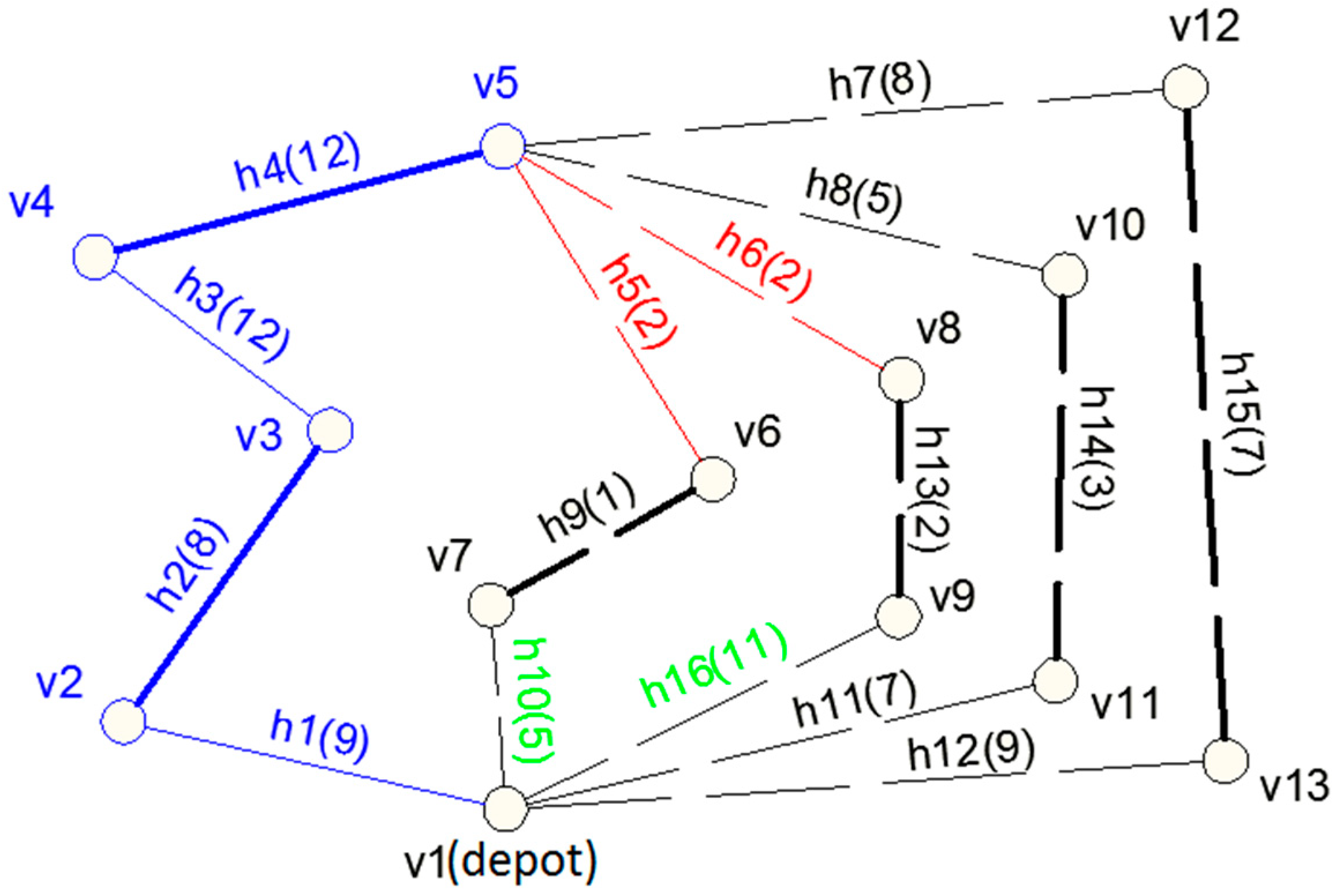
Figure 1 is an example of how the following service edge is selected according to the $cri{t}_1$ criterion. The service edges are marked with a thick line and the minimum unserved routes between the individual service edges with a thin line; $v_1$ depot is in this case also a deposit site. The route ends at the $h_4$ edge. The minimum distance to the service edges that have not been served equals 2, and the set of other potential edges is $Z=\left\{h_5,h_6\right\}$. For the selection of the next service edge of the route, the $cri{t}_1$ criterion is used, which minimises the return to the depot $\left(min\left\{kon\left(h_9\right),kon\left(h_{13}\right)\right\}=min\left\{5,11\right\}\right)$, thereby extending the journey by the $\left(h_9\right)$ edge.

For one selected criterion $crit\in \left\{cri{t}_1,cri{t}_2,cri{t}_3,cri{t}_4,cri{t}_5\right\}$, it is possible to find a solution in $O\left(m_R\right)$ time, that is, in $O\left(n^2\right)$ for a real urban road network with $m_R\le m^{\ast }\approx 4$, where $m_R$ represents the number of service edges and n the number of graph vertices [38,47]. By random selection of the next service edge l on the route [48], it is possible to obtain more than five alternative solutions and improve the average value of a solution.

The first option involves the random selection of one of the five criteria $cri{t}_1\dots ,cri{t}_5$, each one with equal probability, which determines the next service edge l. Another option is to ignore the criteria, and instead of choosing the edge minimising the criterion on the Z set, to perform a random selection of the edge from the set of the nearest edges, Z [7,39].

4. Discussion

Approach methodology for determining the number of mixed waste bins designed within this research study consists of several followed-up steps. Fundamental to determining the number of mixed waste bins was to analyse the waste on the basis of the volumes of household waste produced, according to the type of built-up area and specific components of household waste sought (see Table 1 and Table 2). As mentioned, a rule of thumb used by most waste collection companies is that the average volume of waste produced per person per day is 5 L (see Section 2.2). Subsequently, the weight values were converted to the average values for bulk density in terms of built-up area (see Table 3), as well as individual components (see Table 4).

Based on the share of the individual components, it was possible to calculate the volumes of the individual components then (see Table 5). Additional calculations based on the waste production per person per day, as well as the weight of the individual components, were carried out (see Table 6). The calculation of volume of mixed waste with 50% separation of specified components (see Table 7) and the volume of mixed waste with current levels of separation (see Table 8) were performed. The outcome was to compare the volume of mixed waste under different waste separation levels (see Table 9), whereby it was demonstrated that 50% separation of selected waste types brings up to 50% reduction in the required number of mixed waste bins.

Chapter 3 of this research study is focused on application of the NNS method as a sequential constructive heuristic approach, uniquely implemented to define an optimum frequency of the mixed waste collection cycle within a given predesignated area. Specifically, using this method, the only route with which to cover all service edges in terms of waste bins collection can be found.

In addition to the NNS method, two other optimisation techniques to be applied to a given issue problem may be taken into account as well; namely, Distributing or Two-Phase Heuristic method, and Bellman-Ford Algorithm.

Distributing or Two-Phase Heuristic method consists of two phases and may or may not account for the vehicle capacity. The first phase includes determining the complete route that can be found using any heuristic method, e.g., NNS heuristic. The second phase accounts for the vehicle capacity and specifies the number of waste collection vehicles. In regard to the Bellman-Ford Algorithm, to determine the shortest path, the time demand is considered the key attribute, whereby it is linearly dependent on the number of directed edges of the acyclic graph.

The detailed principles of these method procedures are described as follows (Section 4.1 and Section 4.2).

4.1. Distributing or Two-Phase Heuristic Approach

Under the simplified version (without capacity constraints of the vehicle) only one route, which would include all service edges, can be found. However, with respect to vehicle capacity, this route needs to be subdivided into shorter routes served by individual vehicles so that the required capacity on the routes is not higher than the capacity of the vehicles used on these routes. This is ensured by the next phase of the calculation—the so-called distributing heuristic (hereinafter referred to as DH), or two-phase heuristic [37].

The principle of the two-phase heuristic is to find the complete route $T_1^{X_R}$ that comprises all service edges (regardless of vehicle capacity) and its division into optimum capacity-permissible routes using the DH described in the following paragraph [54]. Dividing the complete route does not ensure the inception of the optimum capacity-permissible route. The complete route can be determined using any heuristic, e.g., NNS heuristic [39].

A DH can be applied to either an oriented, disoriented, or mixed complete route $T_1^{X_R}$, whereby the individual edges are assigned labels representing a connectivity demand or the length of the edge. The capacity of a vehicle is Q. Under the DH, an auxiliary acyclic graph H was created, with $m_R+1$ points with assigned numeric value in ascending order, starting with 0. Each permissible route from the subset $\left\{T_{1i}^{X_R},\dots T_{1j}^{X_R}\right\}\in T_1^{X_R}$ of the complete route is represented by only one or-edge $\left[i-1,j\right]$ in the H graph. The route is permissible if neither the capacity of the vehicle (Q) nor the L driving range is exceeded. The loading volume on the route is calculated as follows [54]:

$$nak\left(T_i^R\right)={\displaystyle \sum }_{j=1}^{m_R}w\left(h_j\right)\le Q\left(h_j\in T_i^R,i=1,\dots ,\left|T_R\right|\right)$$

(1)

The shortest path from the vertex indexed 0 to the vertex indexed $m_R$ in the H graph determines the best possible division of the complete route [52]. By dividing the route, several capacity-permissible routes are established. This results in the optimum solution being found in regard to the sequence of the edges on the original route.

4.2. Bellman-Ford Algorithm

The shortest path can be calculated by means of the Bellman-Ford Algorithm for a directed acyclic graph [52]. The time demand is linearly dependent on the number of directed edges of the graph. For the H graph [51], the maximum number is $\frac{m_R\left(m_R-1\right)}{2}$. Therefore, the time demand is $O\left(m_R^2\right)$. The time demand for a real urban road network with $m_R\le m^{\ast }\approx 4n$ equals $\left(n^2\right)$ [14].

The time demand will be smaller if the $w_{min}$ minimum requirement is large enough. The route thereby optimally covers $\frac{Q}{w_{min}}$ number of service edges. The H graph contains $m_R\frac{Q}{W_{min}}$ or-edges. The time demand of this alternative is $O\left(m_R\right)$, without any need to create the H graph. For $i=1,\dots ,m_R$, all the permissible routes $\left\{T_{1i}^{X_R},\dots ,T_{1j}^{X_R}\right\}$ are labelled. The labelling is used for the direct actualisation of the labelling of the vertices in the Bellman-Ford Algorithm [50,53].

The DH can be improved by dividing several complete routes and choosing the best solution obtained through these divisions. When truncating the capacity (Q) of the vehicle and the driving range (L), the complete routes can be determined using the aforementioned NNS [7]. The NNS heuristic enables the creation of five such routes (one for each given criterion).

Another improvement may be achieved by changing the order of the edges on the route in the H graph. Better results are achieved if each or-edge in the H graph is assigned labelling according to the best cyclic order change of the edges on the route [54].

5. Conclusions

Currently, the issue of the waste separation and collection is considered a very up-to-date topic and a lot of authors in various professional publications have dealt with it (as stated in the literature review within the introduction). A number of research studies elaborate the issues of separated waste production in terms of municipal waste volume reduction. Several authors also point to the fact that the 50% recovery rate has yet to be achieved in EU big cities. Apparently, the municipal waste reduction affects the waste collection cycle of collection vehicles.

However, none of the aforementioned publications and approaches is focused on the issues of the waste separation and collection within one comprehensive methodology. This concern is addressed just within this research study, specifically by its conception. It includes several followed-up steps.

• Analysis of the waste on the basis of the volumes of household waste produced according to the type of built-up area and specific components of household waste;
• Calculating the weight values converted to the average values for bulk density, in terms of built-up area, as well as individual components;
• Calculating the volumes of the individual components;
• Calculating the waste production per person per day, as well as the weight of the individual components;
• Calculating the volume of mixed waste with 50% separation of specified components, as well as the volume of mixed waste with current levels of separation;
• Comparing the volume of mixed waste under different waste separation levels;
• Applying the NNS heuristic to the collection cycle frequency of municipal waste bins in a predesignated urban road network area.

The results achieved within the research confirmed that the number of municipal mixed waste bins can be reduced due to the separation of paper and plastics up to 30–50%. Such a reduction has significant impact on the collection cycle frequency. For that reason, specifying the components in order to achieve the reduction in municipal waste volume, as well as using the proper technique and approach in this matter can considerably streamline the whole waste management system.

As mentioned, the uniqueness of the designed methodology also consists in an application of the specific operational research method (specifically, the Nearest Neighbour Search method as a sequential constructive heuristic approach) in regard to define the optimum frequency of the mixed waste collection cycle for a waste collection vehicle within a given predesignated area. This method determines the only route with which to cover all service edges in terms of waste bins collection. Each service edge must be chosen by minimising or maximising one of the criteria, as follows:

• Minimisation of the evaluation of the route (its length) beyond the service edge to the depot;
• Maximisation of the evaluation of the route beyond the service edge to the depot;
• Minimisation of the ratio expressing the “productivity” of the service edge;
• Maximisation of the ratio expressing the “productivity” of the service edge;
• Criterion 5 = criterion 1, under pre-determined conditions (see Table 10).

Such a methodology has not been published yet. Therefore, the designed technique can be seen as a new or different holistic view for determining the necessary number of municipal mixed waste bins, as well as the optimum waste collection cycle in a variety of municipalities. The next step in the future should be to deal with the financial aspects of the optimum collection cycle of municipal waste management.