Do Amphibians and Cash Crops Compete for Scarce Water? A Spatial Correlation Analysis

Abstract

It has been argued that the trade of water intensive crops may be beneficial as it helps alleviate regional differences in water scarcity by effectively transporting moisture from humid regions to arid ones. However, the incentive to grow export crops can also intensify pressure on local water resources. Water abstraction for use in growing cash crops can affect rivers and wetlands with rich biodiversity reserves. In many macro-level environmental assessments, it is assumed that water use is a proxy for biodiversity pressure. Here we use correlation analysis to test the degree of spatial overlap between areas with high scarce-water consumption for cash crop production (i.e., crops where a majority is exported) and areas with high species richness or vulnerability of Red-Listed amphibians. We find that, globally, there is relatively little spatial overlap between areas where scarce water is used for export production and the habitat range of stressed amphibians.

1. Introduction

Due to the limited availability and uneven distribution of global freshwater resources, water scarcity is recognized as a coming major environmental concern [1,2,3]. Two of the main challenges linked to water scarcity are maintaining food security with increasing water constraints in agriculture while preserving ecosystem health [4]. These sustainability challenges of increased water scarcity, food security, and loss of biodiversity are daunting in isolation, and even more complex when the interconnections and feedback loops between them are considered [5]. Competition for scarce water resources is often framed as occurring at the center of an “energy–food–biodiversity” nexus. Water is needed for energy production (both thermal and biofuel); for food (both staple and cash crop); and for ecosystems. This conceptual framing is well established, but what is needed now is more detailed and quantitative studies revealing how intensely these uses vie for scare water in actual situations.

In this study, we investigate a small part of the complex water–energy–food–biodiversity puzzle, namely the relationship between biodiversity and scarce-water use in the farming of cash crops. Competing demand for scarce water impacts biodiversity health in other ways as well (e.g., drought-prone regions may have to make decisions between urban water use and ecosystem health) but in this study, we focus specifically on testing for a spatial overlap between agricultural production for export and amphibian habitats.

Recent results from the living planet index indicate that freshwater species populations have declined on average by 83% since 1970; a rate of decline steeper than for terrestrial or marine species [6]. Amphibians are affected by surface and ground water depletion and reduced water availability [7,8]. Therefore, it may be assumed, that water consumption in agriculture—the major water consumer globally—competes with these species, and that increased abstraction for agriculture will be likely associated with biodiversity threats. Water-dependent species are, in general, at a greater risk of extinction than land-based species and the primary reason for this trend is habitat change [9,10]. Habitat change is a complex phenomenon, consisting of a mix of direct impacts e.g., by land use and land cover change, and indirect impacts including eutrophication and competition with anthropogenic water abstraction [9]. Due to this complexity, exact environmental impacts to particular species loss are mostly not known, however, it is believed that in most cases, threatened species are affected by multiple drivers at the same time [11,12]. To simplify this complex system, one may ask merely if water withdrawals and scarce-water consumption in agriculture in particular can be used as a proxy for biodiversity threats.

While much of the water is used locally to satisfy domestic needs, it has been estimated that up to one-fifth of the total global water consumption in agriculture is used for production of cash crops or agricultural products traded between countries [13]. It has been argued that trade in water-intensive crops can help alleviate differences in scarcity (i.e., when a humid region exports water-intensive crops to an arid region) [14,15,16]. However, the opposite often occurs, with a net outflow of water embedded in commodities adding pressure on local resources. Another study [17] found that up to one-third of global species threats can be attributed to production of traded commodities. Chaudhary and colleagues studied the biodiversity footprint of agricultural products and found that 95% of the Swiss footprint was exerted in other countries, with cocoa, palm, and coffee being key culprit commodities [18,19]. That study, while closely related to ours conceptually, did not specifically investigate the degree of spatial overlap between species-rich areas and agriculturally rich areas.

Against this background we pose the following research question: Do cash crops (i.e., crops predominantly grown for export) and amphibian species compete for scarce water? To investigate this, we use spatial correlation analysis and test the degree of overlap between areas producing export crops using scarce water and areas experiencing amphibian biodiversity threats. The research question may be stated in terms of two testable and falsifiable hypotheses:

• Areas exporting more scarce water due to cash crop production have a lower amphibian species richness;
• Areas exporting more scarce water due to cash crop production have higher overall amphibian species vulnerability level.

In this study we look at a single-year snapshot and perform spatial correlation analysis to test for the degree of overlap between water demand and sensitive habitat.

As we discuss more fully below, there are also likely inter-temporal and distant spatial relationships between species health and agriculture as well. For example, we could consider two extreme cases. We could imagine a plot of land which is used for just one year to grow a crop and that crop disrupts a particular species’ life-cycle. However, the impact on the species becomes only visible several years later. Likewise, agricultural runoff from say a coffee plantation could flow downstream and create impacts in a different model grid cell than the farm. In both cases, there would be a relationship between cash crop production and species health, but spatial correlation analysis would not capture it. Modeling these two effects is challenging for two reasons: First, because spatially explicit, year-over-year data on species health is essentially non-existent; and second, because even if data challenges could be overcome it is not necessarily straightforward to attribute a species threat to a particular activity. Thus, while acknowledging that spatial correlation is a primitive tool to test the relationship between cash crop production and species health, we argue that it is practical and can provide interesting and meaningful results. In an ideal situation temporal analysis would also be used, but for lack of data no temporal analysis is conducted in this study.

2. Materials and Methods

We propose and test the two hypotheses outlined above using spatial correlation analysis. The aim is to understand the extent of overlap between regions rich in amphibian biodiversity and regions with high use of scarce-water consumption for exported cash crops.

We do this by graphic analysis using scatterplots and by correlation maps. The software used in these analyses were Matlab and ArcGIS. With scatterplots, each point is a grid cell (map pixel) and the two axes measure the biodiversity value of the cell and scarce-water use within that cell. If the same cells have both high biodiversity value and high scarce-water use, the scatterplots will show points falling along the 45° line. If there is little overlap—that is, a cell is either home to more species or high in water use, but not both—the scatterplots will show points falling along the horizontal and vertical axis edge in the charts and not along the 45° line. For the correlation maps, we used the same data and set threshold levels that help visualize the spatial overlap between water use and biodiversity richness. We measure three variables: (a) The total scarce-water consumption of cash crops, (b) amphibian species richness, and (c) amphibian species vulnerability level.

The year studied was 2000. While investigating a more recent year would obviously be preferable, we had several reasons for not doing so. The most significant is that information for biodiversity, from the IUCN Red List, does not have an explicit temporal dimension, since it is updated on a rolling and irregular basis. The Red List version used nominally holds for the year 2000. Furthermore, the water use data from the Water Footprint Network are referenced to 2000 as the base year. Water demand for other years could be modeled or estimated but this would introduce another source of uncertainty. Finally, patterns of both cropping (the dominant crops in a region) and biodiversity change relatively slowly, often on the scale of decades or longer.

A temporal analysis would also be another way to look at the relationship between water use and amphibian health, and to start to look at explicit causal relationships (i.e., does scarce-water use cause biodiversity harm), but assembling suitable measures of biodiversity health and water usage over large spatial scales is exceedingly challenging, and was outside the scope of the present study. The static single-year analysis already provides a useful insight into the degree of competition, or non-competition, between water use and amphibians.

The spatial correlation analysis was conducted at a resolution of 5 arc min (cells are approximately 10 km² at the equator). The limitations of the results due to spatial resolution are discussed below.

Data about yearly scarce-water consumption (SWC) of global agricultural crops (i.e., the amount of scarce water that is not returned to the original source after being withdrawn) were provided by Pfister and colleagues [20]. To account for scarce-water volume, Pfister uses the RED water (relevant for environmental deficiency) concept representing amount of water deficit that is abstracted and not available to downstream human and ecosystems uses. The data covers 160 different crops and has a spatial resolution of 5 arc min. Water-consumption data was taken for the year 2000. Water-use data for other years is not regularly available so it must be estimated.

To compute the amount of water consumed by cash crops, we multiplied the water used to produce the entire growth of a given crop by the share of that crop which was exported. Data on crop production and exports for each country were taken from the Food and Agriculture Organization of the United Nations, Statistics Division (FAOSTAT) reflecting international trade of commodities in the year 2000.

We estimated the scarce-water demand for production of a cash crop c in each grid cell by multiplying the [scarce water demand per ton of production of crop c, from Pfister et al.] * [tons of production of crop c] * [ratio of total national exports of crop c to total national production of crop c]. All cash crop water consumption datasets were summed to get the total scarce-water consumption of all crops grown for export in year 2000.

We note that in the FAOSTAT data, a country can export more of a particular crop than it has produced in that particular year. This can occur because the export is sold from stocks or when the country is a middle trading partner re-exporting agricultural production with a foreign origin. In this study, in a case when a country’s production was 0, but export was reported, export intensity was set to 0%. In the case of reported production quantity lower than the export quantity, all export intensities were set to 100%. This situation occurs rarely (<≈1% of records).

To measure the state of amphibian biodiversity, global maps of amphibian species richness (SR) (number of species) and vulnerability score (VS) of these species (a function of their total range area and IUCN threat levels) were taken from Reference [21] who model a “vulnerability score” per species based on its threat level and range area. Note that vulnerability here refers to the likeliness to become endangered or extinct, not to be confused with the IUCN’s “VU (Vulnerable)” risk category. Both maps have been made based on IUCN Red List data of threatened species. The species-richness map was made by adding up individual species geographical extents of distribution and species presence categories ‘extant’, ‘probably extant’, and ‘possibly extant’ using the extent-of-occurrence maps from the IUCN. The origin of species, or the difference whether species are native or introduced, was not considered. The vulnerability level is a score ranging from 0 (not vulnerable) to 1 (highest vulnerability) and is defined as a function of extent of occurrence and threat level. The extent of occurrence serves as a proxy measure of susceptibility to anthropogenic disturbance since species with small range are intrinsically rare and could be more easily driven to extinction. Threat level, in contrast, measures only already occurring threats. Thus, this score indicates the already existing risk of becoming extinct through the threat level (how close to extinction is it already?) and gives an indication on the potential future increases in threat level if the species loses habitat (i.e., a small-ranged species that is losing habitat is more likely to move closer to extinction than a large-ranged one, since the former has limited remaining habitat area to move to). Taking both aspects into account instead of just backward-looking threat levels (existing threats) is important for environmental assessments, thus we chose to apply the VS instead of just the threat level.

Our chosen approach is subject to limitations which may affect the results. Some of the important limitations include:

-

Trade data from FAOSTAT contains inaccuracies.

-

Crop water demand is estimated via a model, and that model may contain inaccuracies.

-

The species extent-of-occurrence maps from IUCN may not be completely accurate. Additionally, the extent-of-occurrence maps from IUCN show the maximum range of each species but not their distribution within that range. It may be that a species is only rarely observed in one area, and still the species extent-of-occurrence map will be expanded to include that point, while in fact the species is predominantly residing in another area. This could bias the results reported in this paper both ways: A grid cell reporting a water use/species overlap could be either intensely, or merely sparsely, populated by that species.

-

The species vulnerability is estimated using a model; that model may not correctly report species vulnerability.

-

There may be observation bias in the species occurrence or extent-of-occurrence data, as the robustness of biodiversity monitoring and mapping varies considerably by country and by species. Furthermore, not all species might be reported and have geographic data available.

-

The spatial units are relatively big, at 5 arc min. It could be that production of an export crop, use of scarce water, and residence of vulnerable species all occur in a single grid cell but at different locations within it, in which case our results would show an overlap when in reality no such overlap exists. This could systematically bias our results to show more water/biodiversity conflict than really exists. To a degree the results presented here are sensitive to the selected gird cell size: If the entire planet were mapped as one grid cell, there would be 100% overlap, while at the other extreme if the spatial unit were 1 m² it would be quite unlikely to find amphibians residing essentially directly underneath commercial crops.

-

Downstream impacts are not considered. The map of water demand looks at where crops are produced, not where that scarce water comes from. It could be that the use of scarce water for cash crop production induces water scarcity and pressure on amphibians upstream or downstream, and the method used here may not report an overlap between cash crop production and species in those grid cells.

-

Water use, cropping decisions, and species ranges shift over time. Our study is conducted for the reference year 2000, but the data on water use, spatial crop production patterns, and species ranges, are all estimated and likely not very sensitive to yearly fluctuations. These short-term fluctuations and the difficulty measuring this input information could mean that our results are not representative of an average year but rather reflect a particular set of data years in which there was particularly much, or particularly little, water/biodiversity conflict. According to the statistical principle of the law of large numbers, such short-term fluctuation effects should cancel out over a global dataset and study, though there remains a possibility that such short-term fluctuations affect our results.

-

This study only uses a specific way to measure both biodiversity health and water use due to cash crop consumption. It could be that different empirical measures of these two phenomena would reveal different results.

-

As mentioned above, we did not investigate causal or intertemporal effects. Many impacts on biodiversity are slow, cumulative, and/or delayed. It could happen that agriculture activity does impact amphibian health, but that these effects accumulate slowly or are delayed and, thus, are not visible with the measures of biodiversity health applied in this study.

-

There may be significant domestic trade within large countries. In this study, the research question is focused on crop production for foreign export, so we have not looked for overlap between amphibians and scarce-water use for domestic production.

3. Results and Discussion

Here we present the results from the correlation analysis and discuss the findings. This section is organized in terms of testing the two proposed hypotheses, and investigating the Western Ghats—a rainy, tropical mid-elevation biome in South-western India—as a case study, which are interesting as they sharply differ from the global pattern.

One possibility is that biodiversity health improves. Agriculture provides habitat to amphibians, for example in coffee and tea plantations [22,23] and, in cases, in rice fields [24,25].

Furthermore, while the term “invasive species” has a negative connotation, a shift in water regime could make it possible for new species to expand into an area.

3.1. Global Correlation

3.1.1. Testing a Hypothesis: Do Areas Exporting more Scarce Water due to Cash Crop Production have Lower Amphibian Species Richness?

The first hypothesis tries to address the main research question: Do cash crops and species compete for scarce water? Amphibian species richness is used as one measure of biodiversity following an assumption that areas with higher scarce-water consumption will have higher pressure on amphibian ecosystems and this will lead to less amphibian species.

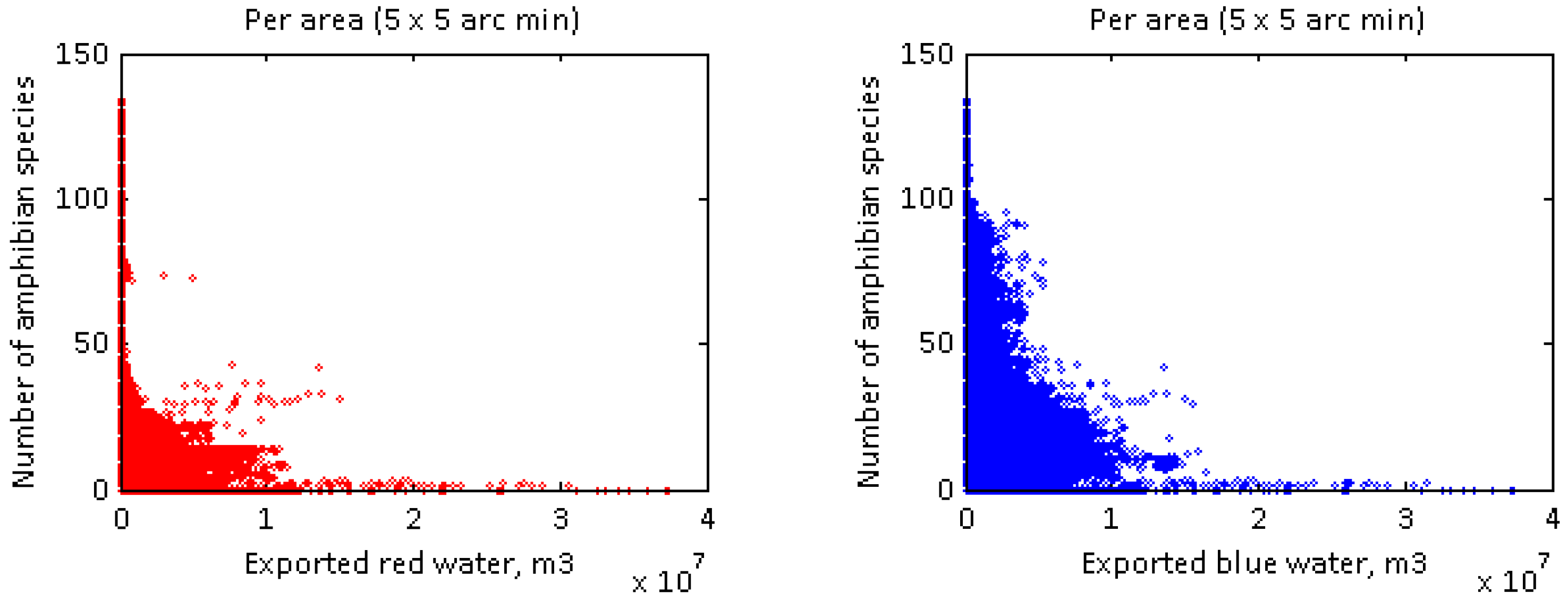
If this hypothesis is true, we expect to see a positive correlation between scarce-water consumption and amphibian biodiversity. This was not observed in the results (Figure 1).

In the correlation results (Figure 1), it can be seen that areas with higher scarce-water consumption are home to fewer amphibians. The areas with the highest amphibian species richness use an average or below-average amount of blue and red water for cash crop production.

There are large variations globally. In some grid cells, there is zero scarce-water consumption but approximately 40 amphibian species present, which is well above the mean global value of 14 species inhabiting a grid cell. At the same time, another area can also have 40 species while production there annually consumes >10 Mm³ of scarce water. This suggests that amphibian health is more governed by other factors, which may include climatic and environmental conditions, crop type, and crop production system, among others.

The results show that species richness is highest in areas where there is very low or zero scarce-water consumption for cash crop production. There are no areas in the world with high scarce-water consumption and exceptionally many (>50) amphibian species. In contrast, we observe very few amphibians inhabiting the areas with the highest scarce-water use. In Figure 1, we can read these trends by seeing the very long tails close to the horizontal and vertical axes.

It is interesting to see the difference between correlation patterns for scarce (red) and blue water. Figure 1 reveals that more amphibian species live in areas producing blue water intensive cash crops than areas that use the same amount of red water. From the correlation graphs, this means that an area on the global map which produces cash crops consuming 1,000,000 m³ of blue water annually can host up to 100 amphibian species but no more than 50 species if this water is scarce.

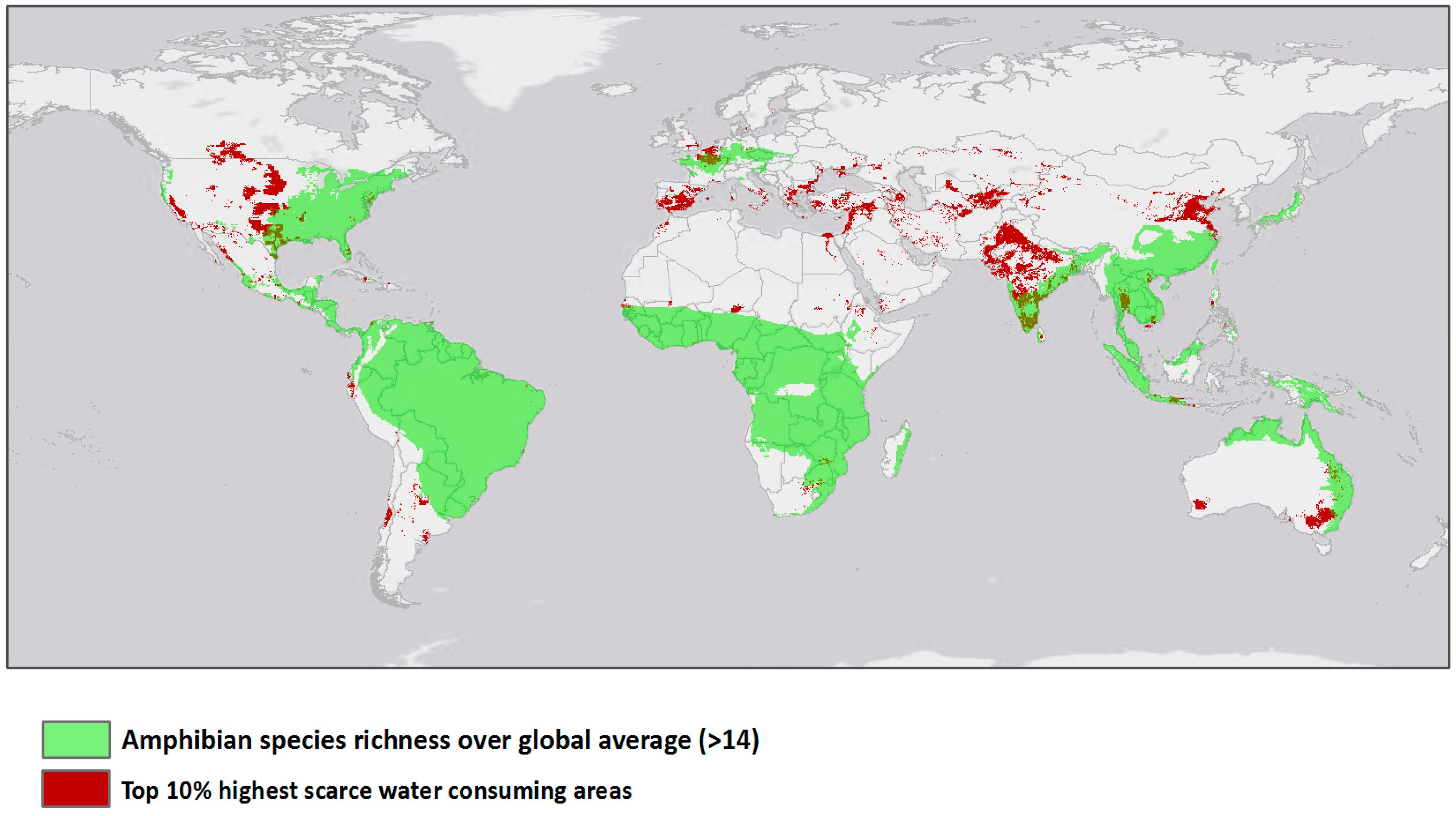
The correlation patterns may also be investigated visually in a map. Maps can help reveal the spatial patterns of the (inverse) correlation. The map in Figure 2 shows the top highest scarce-water-consuming areas globally (dark red color) and areas with amphibian richness above the global average of 14 species (green). We can clearly see that most of these areas do not overlap. This means that, in areas where scarce-water-intensive cash crops are produced, amphibian species richness is generally low. Many of the high scarce-water-consuming areas are arid like Central Asia, Middle East, and large parts of Australia, and, naturally, have lower amphibian richness than in wet tropical regions. This suggests that one of the reasons why there are lower amphibian richness in scarce-water-consuming areas (seen in the correlation graphs before) is that most of these areas are located in arid regions naturally having less amphibian species.

From this, we can conclude that, when considering purely species richness and no other biodiversity aspects, scarce-water-intensive cash crops do not compete with amphibian biodiversity. Trade-offs to amphibians in areas producing water-intensive cash crops in most cases will not be massive on a global scale if production is continued in the present agricultural areas.

In spite of this general trend, there are many variations globally. Figure 3 shows areas with high scarce-water consumption and shows the amphibian species richness in these areas. The results show that areas growing cash crops with high scarce-water consumption can have (1) no amphibians (areas in orange), (2) low amphibians species richness, here, species richness below the global average (areas in green), and (3) high amphibian species richness, here, species richness above the global average (areas in pink). The difference between the two maps is the threshold level chosen for scarce-water consumption. The upper map (Figure 3A) shows areas in the top decile of scarce-water consumption for export crops. The lower map (Figure 3B) shows a larger area: All cash crop production areas with scarce-water consumption above the global average level (global average = 7025 m³ per grid cell) in 2000.

The Central Asian countries Uzbekistan, Kyrgyzstan, Tajikistan, and Turkmenistan are some of the most scarce-water-intensive cash crop-producing areas globally (see areas in orange). In these countries, up to 90% of all water withdrawals are used in agriculture, notably cotton production [26].

Raw cotton is the most important agricultural export commodity earning from more than 40% of export income in Uzbekistan to 7% in Kyrgyzstan in the year 2000 (FAO, FAOSTAT database). At the same time, we can see that cotton production does not compete with local amphibian biodiversity in this area because there are simply very few amphibians.

In this study, it is not investigated whether amphibians have been lost in the past due to water abstraction. However, according to the IUCN Red List, none of the recorded 38 amphibian species extinctions are recorded in Central Asia [27].

The maps show that with an increase in scarce-water consumption, a smaller proportion of areas have above-average species richness. In Figure 3B, most areas in pink are classified as having little or no physical water scarcity according to the UN [26]. These include Southeast USA, Brazil, Eastern Australia, Western Europe, and most pink areas in Africa. With the increase in scarce-water consumption (Figure 3A), most of these areas disappear.

In Figure 3A, some ‘hotspots’ come out where area sustain amphibian richness over global average and at the same time large amounts of scarce water is consumed to grow cash crops. Most of these areas are in South Asia, especially India. We may also ask whether many amphibian species can live in these areas because of crop systems that provide good habitat to many species and other favorable factors? Or are these diverse amphibian communities more threatened than in areas with lower pressures from scarce-water consumption? These questions cannot be investigated looking at species richness alone. Therefore, the investigation is continued using another biodiversity metric: The vulnerability level of amphibians, a metric that attempts to measure the extinction risk facing a species.

3.1.2. Testing a Second Hypothesis: Do Areas Exporting more Scarce Water due to Cash Crop Production have a Higher Overall Amphibian Species Vulnerability Level?

In this section, we use a species vulnerability score [21,28], an alternative to species richness, to measure the sensitivity of amphibians in an area. The vulnerability score reflects the overall likeliness that an amphibian community in an area may become endangered or extinct. This measure is composed of data about extent of occurrence and threat level of individual amphibian species. While we might expect that the vulnerability level of amphibians living in areas with high scarce-water consumption for cash crops will be higher, the results suggest that globally this is not the case. This piece of evidence invalidates Hypothesis 2.

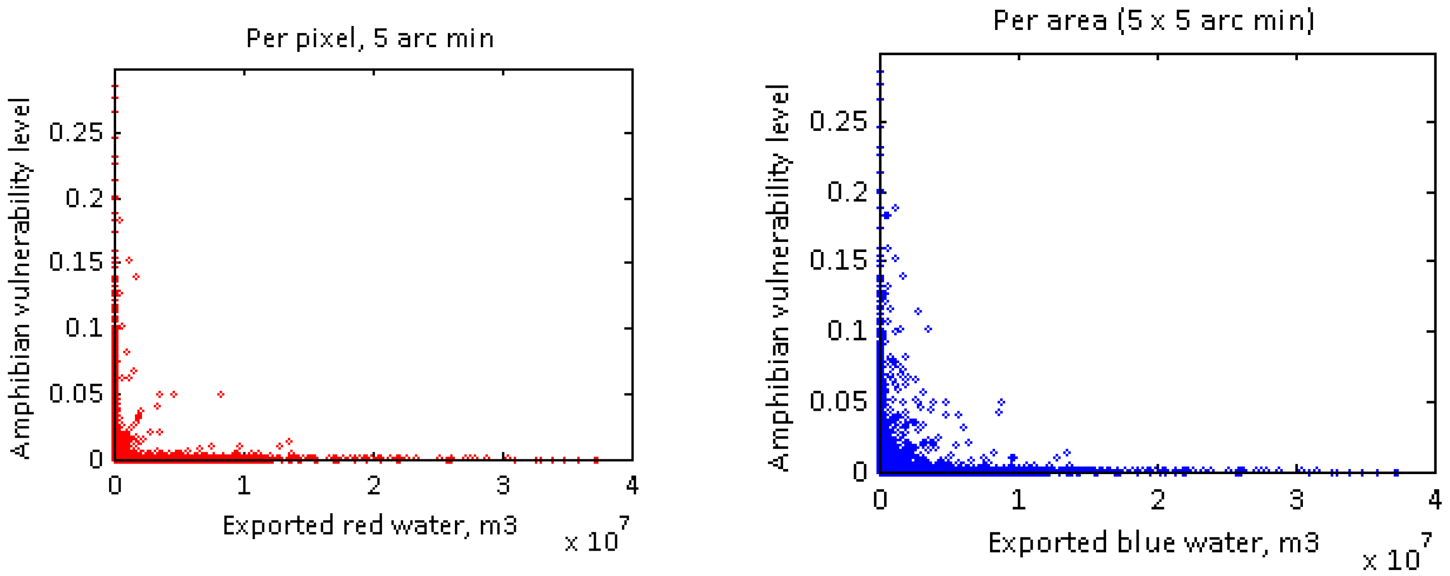
The scatterplots in Figure 4 plot the vulnerability score in each grid cell against the scarce and total water use in that grid cell. The results show that the most vulnerable species (high vulnerability score) tend to reside in areas with very low or zero scarce-water consumption for cash crops. Furthermore, the areas with the highest scarce-water use for cash crops are not home to communities with high vulnerability scores.

Even though we might expect that the vulnerability level of amphibians living in areas with high scarce-water consumption will be higher, results suggest that globally this is not the case, therefore disproving the Hypothesis 2.

In most areas of the world, the amphibian vulnerability score is low. This is seen by the many grid cells having a vulnerability score less than 0.05. If Hypothesis 2 was correct, we would see an increase in mean vulnerability score in grid cells that use more scarce water for exports. This is not observed in the results in Figure 4.

A comparison of red-water and blue-water correlation graphs in the left and righthand panel of Figure 4, respectively, shows that while vulnerable amphibians tend not live in areas with high scarce-water consumption, there are more areas globally with high blue-water consumption and vulnerable amphibians. There is also more variation in the relation of the two, indicating that vulnerable amphibians live in areas with no blue-water consumption as well as in areas with low and high blue-water consumption for cash crops.

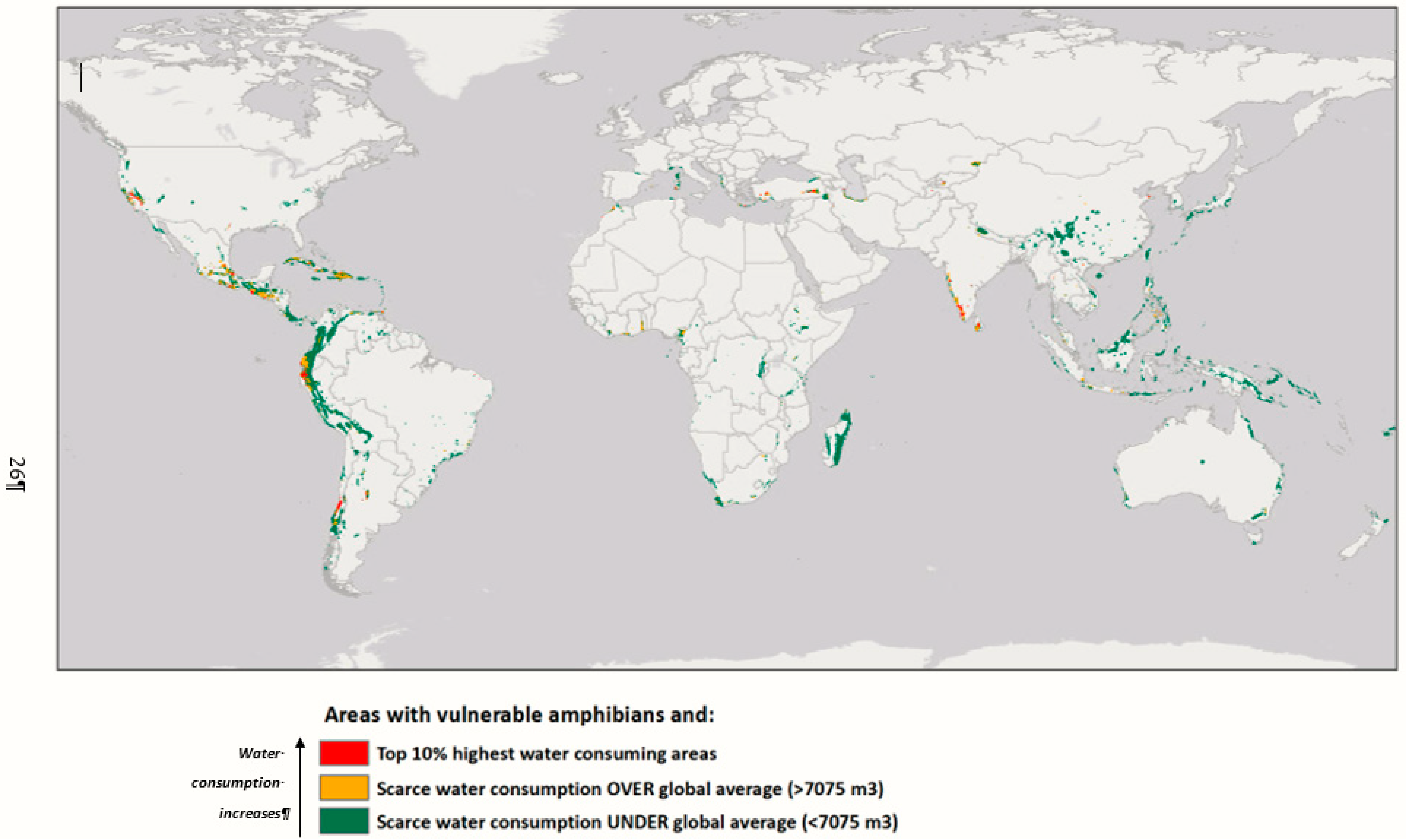
Figure 5 provides a correlation map showing amphibian vulnerability vs. scare-water consumption for cash crops. It shows the main trend of relation between the two variables discussed earlier as well as exceptions. All colored areas in the map are where vulnerable amphibian communities are located, defined as species with a VS >= 0.001, which is the global average VS.

Distribution of vulnerable amphibians largely follow the location of areas with exceptional concentrations of endemic species and exceptional loss of habitat, or so-called biodiversity hotspots [29,30]. As we can see, most of these areas have low scarce-water consumption reflecting the major trend from the correlation graphs that most areas with vulnerable amphibians do not have scarce-water-intensive agriculture. At the same time, there are exceptions (areas in red and orange).

Areas in red and orange (Figure 5) are the exception to other areas globally and lend support to Hypothesis 2. We can highlight five areas that are both ‘biodiversity hotspots’ and have high scarce-water consumption: The Western Ghats and Sri Lanka in South Asia, Western Ecuador, Mesoamerica covering Central America and some areas in the California Floristic Province, and the Caribbean.

In the previous section, areas having both high amphibian species richness and high scarce-water consumption were identified (Figure 3). We asked, what is the vulnerability level of amphibians in these areas? When comparing correlation maps of species richness and vulnerability level, only one biodiversity hotspot comes out; the Western Ghats and Sri Lanka. According to the results, this area in India and Sri Lanka, which has high amphibian diversity, was one of the top exporters of scarce water embodied in cash crops. These amphibians are also vulnerable.

What are the reasons for this exceptional relation between scarce-water intensive-agriculture and amphibians in this particular area? In the following section, this will be investigated by looking at the Indian part of the ‘hotspot’, the Western Ghats.

3.2. Investigating an Exception: The Western Ghats, India

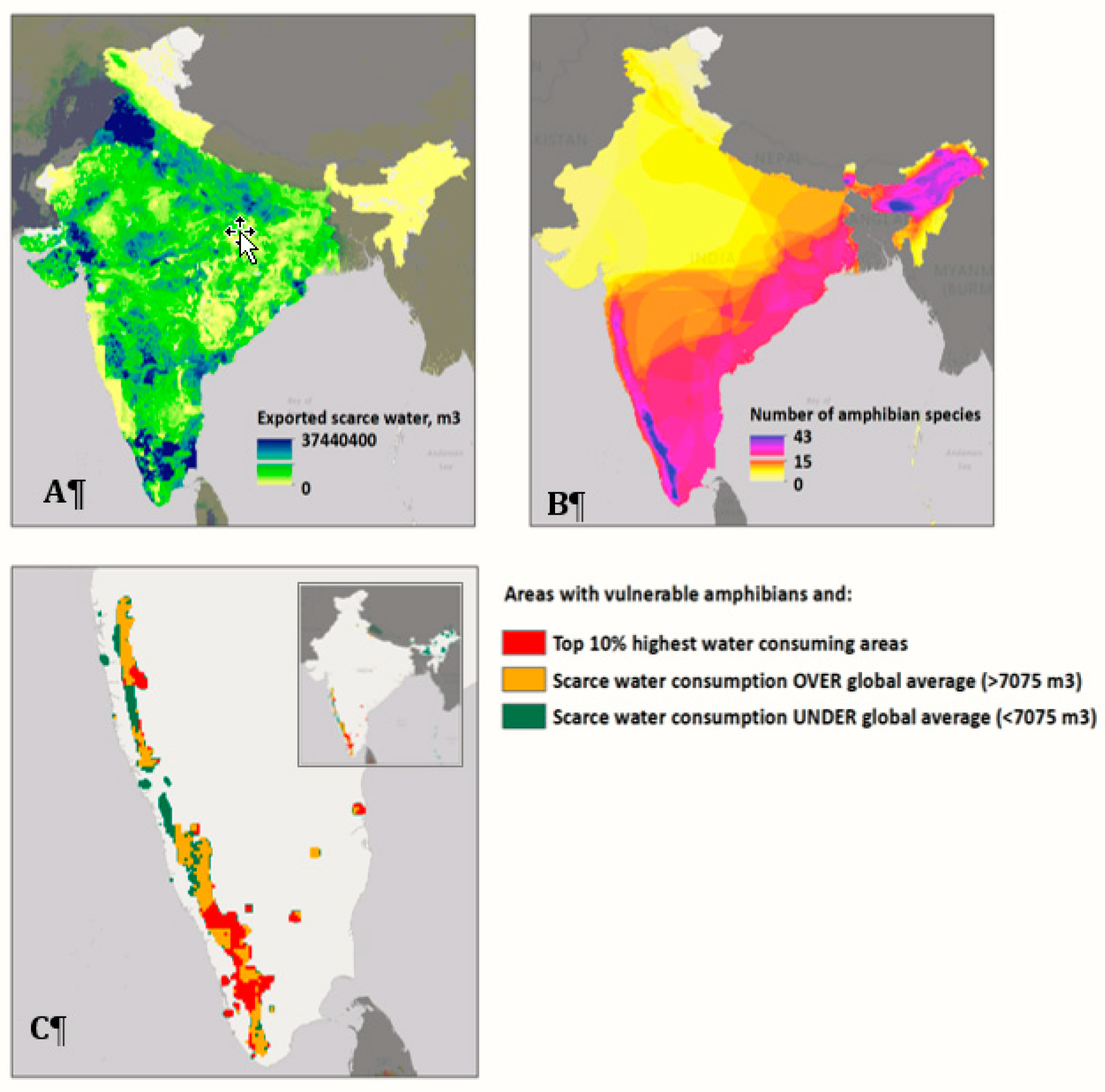
The Western Ghats is a mountain range located along the Southwestern coast of India, in the area around Kerela. The region is semitropical. It is agriculturally very productive, with many tea plantations and mixed spice crops. It is also high in biodiversity. It is recognized as one of the 25 biodiversity hotspots in the world [29,31]. The approximate location of the biodiversity hotspot can be well seen as the amphibian rich area on the West coast of India in the map B and colored area with vulnerable amphibians in the map C (Figure 6). As found from the global correlation analysis, it is an exceptional territory globally for several reasons:

(1)

The Western Ghats has exceptional amphibian species richness, and most amphibian communities in the area are vulnerable;

(2)

India is one of the countries exporting most scarce water embodied in cash crops and some of the most intensive scarce-water-consuming areas are within Western Ghats.

Therefore, according to the results of this study, it is the largest area globally where three variables are present: High scarce-water consumption, high amphibian species richness, and high vulnerability level of amphibian species.

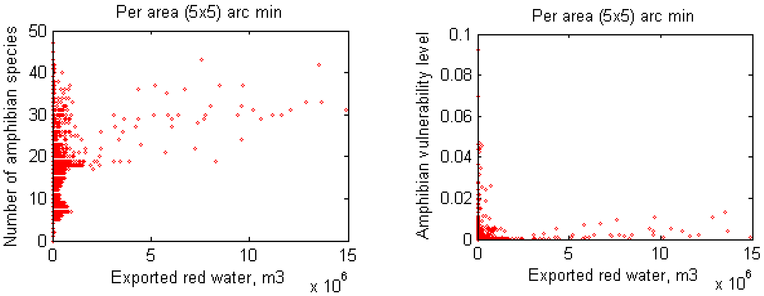
Figure 7 shows the correlation between scarce-water exports and amphibian biodiversity variables in India. In contrast to the situation at the global level, where there is little overlap between thirsty cash-crop regions and amphibian hotspots, in India we see slightly more overlap between the two areas. In particular, the cells with the highest use of exported red water are home to a high number of amphibian species (Figure 7, left panel). However, when adjusted for vulnerability score, we see again the pattern observed at the global level: The areas with the highest vulnerability score are not those with the highest red water use for export crops, and vice versa (Figure 7, right panel). Looking into this more closely using the overlap maps from Figure 6, we identify that most of these ‘exception’ areas are in the Western Ghats.

The Western Ghats is one of the most fragmented and densely populated hotspots, and most of the natural forest vegetation has been cleared to make space for agriculture. At the same time, the Western Ghats has at least 121 species of amphibians, 78% of them endemic [22]. The area is mountainous and receives heavy precipitation, however, only small quantities of water remains in headwater basins due to steep slopes. Agriculture in many valleys is supported by irrigation using surface waters from rivers as well as groundwater. Irrigation has increased crop yields in the area but has also caused disparity in water availability between irrigated and non-irrigated areas [32].

Results show that scarce-water consumption due to cash-crop growing is high in the Western Ghats area with an extremely high scarce-water footprint in the southern part. Various crops are grown but the three leaders are coffee, tea, and rice. From these crops, most scarce water is consumed by coffee. One explanation of this is that coffee plants generally need large amounts of water. Usually, plantations get enough water from precipitation (like in South America). In India, however, rainfall pattern is defined by the monsoon and for four to five months, coffee trees are under drought conditions and are irrigated to secure high yields. This leads to high consumption of surface and ground water. Secondly, according to the cash crop analysis, coffee was the most exported food commodity in India in year 2000 (55% of coffee beans were exported), followed by different spices, such as pepper and nutmeg, and tea with an export intensity of 24%. At the same time, large amounts of food crops in India are used to feed domestic population, and only 1% of rice was exported in the year 2000, leading to low contribution of rice in the total scarce-water footprint of Indian cash crops.

So how can so many amphibian species remain in Western Ghats in areas with scarce-water-intensive agriculture? Are these amphibian species vulnerable because of scarce-water abstraction from their habitats in favor of agriculture? The answers to these questions are undoubtedly complex, but several studies provide relevant explanations.

Canopy cover is the most important factor determining amphibian richness and abundance in Western Ghats [33]. Forests are highly fragmented and shaded plantations of coffee gives refuge for forest biota and act as corridors sustaining connectivity between patches of forest [23]. High amphibian diversity can also be found in tea plantations in the Western Ghats [22], and rice fields and irrigation channels have been recognized as important habitats for amphibians in areas where wetlands have been converted to agriculture [24,25]. Vulnerability of amphibians in the Western Ghats hotspot comes mostly from the small ranges of endemic amphibians. Patchy distribution of amphibian species could have evolved because of forest loss [34], partly caused by expansion of coffee, known to be grown on previously forested areas [35]. Pollution could also potentially contribute to the threat level of amphibians, but the impact of pollution from agriculture in Western Ghats is still not clear. Abnormalities in frogs have been found in coffee and rice plantations in the Western Ghats [36]. At the same time, another study [22] found high amphibian diversity without abnormalities in tea plantations known for heavy pesticide use.

When looking at all these aspects, we are able to conclude that some agricultural systems can play an important role in sustaining amphibians, including vulnerable amphibian communities. In the highly fragmented and deforested Western Ghats, coffee and tea plantations can give refuge to amphibians. It is also important to note here that amphibians are not always deprived from water when water flows are diverted from natural habitats to agriculture. The irrigated rice fields are a good example of a valuable habitat to many amphibians. At the same time, water abstraction in the Western Ghats, the source of many rivers in India, can potentially influence downstream regions with less precipitation as well as deplete groundwater resources. These effects are not considered in this study but should be taken into account in the future research investigating the link between scarce water and amphibian biodiversity.

4. Conclusions and Outlook

The aim of this study was to investigate a part of the complex water–food–biodiversity puzzle by answering the question: Do cash crops and species compete for scarce water? To do so, the correlation between scarce-water use in cash crop production and the state of amphibian biodiversity was examined.

Our results indicate that there is an overall global tendency for scarce-water-intensive cash crops to be produced in areas where low numbers of amphibian species live. Thus, cash crops, if continuously grown in these areas, will not compete with amphibian richness. Furthermore, possibly because of more advanced prior depletion, cash crops do not compete with vulnerable amphibians, which live in areas with minimal or no cash crop production at all.

However, there are exceptions globally where scarce-water-intensive cash crop production, rich amphibian diversity, and vulnerable amphibians coexist. Cash crops may not only deprive amphibians from scarce-water resources, but also in some areas play an important role in giving home to amphibians where their natural habitat is lost. We also note that this study is subject to a number of limitations, as discussed above, so we would urge caution and further study before drawing stronger conclusions or taking action based on these preliminary results.

Scarce-water use might, in regions, also lead to no predictable change in biodiversity health. This could happen for several reasons. There could be no spatial overlap within the grid cell being studied: Scarce water and amphibians occupy different areas e.g., semi-arid zones with scarce water but no amphibians. Biodiversity health could change for other independent reasons. Land-use change is one of the largest causes of biodiversity loss in general [37]. It could be that land use change, rather than water use, is the dominant reason for more robust amphibian species to remain and vulnerable ones to disappear. It could also be that amphibian species in the area have already stabilized, and the remaining species are robust against further changes in human water use. It may be that in areas with a high intensity of agriculture, only the more robust amphibian species with high tolerance of changes in water availability are left. The more sensitive amphibians may have already disappeared in areas where agriculture has created water scarcity. This is the “prior depletion” hypothesis.

Although no causal links are established, this study can suggest potential hotspots for further local investigations looking at the relationship between water scarcity and biodiversity. For improving future analysis, downstream effects of water consumption should be accounted for and trend data used to see scare water consumption versus biodiversity changes over time.

References

- Shiklomanov, I.A.; Rodda, J.C. World Water Resources at the Beginning of the Twenty-First Century; Cambridge University Press: Cambridge, UK, 2003; ISBN 0521820855. [Google Scholar]
- Oki, T.; Kanae, S. Global hydrological cycles and world water resources. Science 2006, 313, 1068–1072. [Google Scholar] [CrossRef]
- Vorosmarty, C.J.; McIntyre, P.B.; Gessner, M.O.; Dudgeon, D.; Prusevich, A.; Green, P.; Glidden, S.; Bunn, S.E.; Sullivan, C.A.; Liermann, C.R.; et al. Global threats to human water security and river biodiversity. Nature 2010, 467, 555–561. [Google Scholar] [CrossRef] [Green Version]
- Postel, S.L. Entering an era of water scarcity: The challenges ahead. Ecol. Appl. 2000, 10, 941–948. [Google Scholar] [CrossRef]
- Liu, J.; Mooney, H.; Hull, V.; Davis, S.J.; Gaskell, J.; Hertel, T.; Lubchenco, J.; Seto, K.C.; Gleick, P.; Kremen, C.; et al. Systems integration for global sustainability. Science 2015, 347, 1258832. [Google Scholar] [CrossRef] [PubMed]
- Harrison, I.; Abell, R.; Darwall, W.; Thieme, M.L.; Tickner, D.; Timboe, I. The freshwater biodiversity crisis. Science 2018, 362, 1369. [Google Scholar] [PubMed]
- Lévêque, C.; Balian, E.V.; Martens, K. An assessment of animal species diversity in continental waters. Hydrobiologia 2005, 542, 39–67. [Google Scholar] [CrossRef]
- Balian, E.V.; Segers, H.; Lévèque, C.; Martens, K. The Freshwater Animal Diversity Assessment: An overview of the results. Hydrobiologia 2008, 595, 627–637. [Google Scholar] [CrossRef]
- Millennium Ecosystem Assessment (MEA). Ecosystems and Human Well-Being: Synthesis Report; Island Press: Washington, DC, USA, 2005. [Google Scholar]
- World Wildlife Fund. Living Planet Report; World Wildlife Fund: Gland, Switzerland, 2014. [Google Scholar]
- Sodhi, N.S.; Bickford, D.; Diesmos, A.C.; Lee, T.M.; Koh, L.P.; Brook, B.W.; Sekercioglu, C.H.; Bradshaw, C.J.A. Measuring the Meltdown: Drivers of Global Amphibian Extinction and Decline. PLoS ONE 2008, 3, e1636. [Google Scholar] [CrossRef]
- Dirzo, R.; Young, H.S.; Galetti, M.; Ceballos, G.; Isaac, N.J.B.; Collen, B. Defaunation in the Anthropocene. Science 2014, 345, 401–406. [Google Scholar] [CrossRef] [Green Version]
- Hoekstra, A.Y.; Mekonnen, M.M. The water footprint of humanity. Proc. Natl. Acad. Sci. USA 2012, 109, 3232–3237. [Google Scholar] [CrossRef] [PubMed] [Green Version]
- Allan, J.A. Virtual Water: A Long Term Solution for Water Short Middle Eastern Economies? Water Issues Study Group, School of Oriental and African Studies, University of London: London, UK, 1997. [Google Scholar]
- Chapagain, A.K.; Hoekstra, A.Y.; Savenije, H. Water saving through international trade of agricultural products. Hydrol. Earth Syst. Sci. 2006, 10, 455–468. [Google Scholar] [CrossRef] [Green Version]
- Yang, H.; Wang, L.; Abbaspour, K.; Zehnder, A. Virtual water trade: An assessment of water use efficiency in the international food trade. Hydrol. Earth Syst. Sci. 2006, 10, 443–454. [Google Scholar] [CrossRef]
- Lenzen, M.; Moran, D.D.; Kanemoto, K.; Foran, B.; Lobefaro, L.; Geschke, A. International trade drives biodiversity threats in developing nations. Nature 2012, 486, 109–112. [Google Scholar] [CrossRef]
- Chaudhary, A.; Pfister, S.; Hellweg, S. Spatially Explicit Analysis of Biodiversity Loss Due to Global Agriculture, Pasture and Forest Land Use from a Producer and Consumer Perspective. Environ. Sci. Technol. 2016, 50, 3928–3936. [Google Scholar] [CrossRef]
- Chaudhary, A.; Brooks, T.M. Land Use Intensity-Specific Global Characterization Factors to Assess Product Biodiversity Footprints. Environ. Sci. Technol. 2018, 52, 5094–5104. [Google Scholar] [CrossRef]
- Pfister, S.; Bayer, P.; Koehler, A.; Hellweg, S. Environmental Impacts of Water Use in Global Crop Production: Hotspots and Trade-Offs with Land Use. Environ. Sci. Technol. 2011, 45, 5761–5768. [Google Scholar] [CrossRef]
- Verones, F.; Saner, D.; Pfister, S.; Baisero, D.; Rondinini, C.; Hellweg, S. Effects of consumptive water use on wetlands of international importance. Environ. Sci. Technol. 2013, 47, 12248–12257. [Google Scholar] [CrossRef]
- Ranjit Daniels, R.J. Impact of tea cultivation on anurans in the Western Ghats. Curr. Sci. 2003, 85, 1415–1422. [Google Scholar]
- Anand, M.O.; Krishnaswamy, J.; Kumar, A.; Bali, A. Sustaining biodiversity conservation in human-modified landscapes in the Western Ghats: Remnant forests matter. Biol. Conserv. 2010, 143, 2363–2374. [Google Scholar] [CrossRef]
- Duré, M.I.; Kehr, A.I.; Schaefer, E.F.; Marangoni, F. Diversity of amphibians in rice fields from northeastern Argentina. Interciencia 2008, 33, 523–527. [Google Scholar]
- Maltchik, L.; Rolon, A.S.; Stenert, C.; Machado, I.F.; Rocha, O. Can rice field channels contribute to biodiversity conservation in Southern Brazilian wetlands? Rev. Biol. Trop. 2011, 59, 1895–1914. [Google Scholar]
- World Water Assessment Programme (WWAP). The United Nations World Water Development Report 4: Managing Water under Uncertainty and Risk; WWAP: Paris, France, 2012. [Google Scholar]
- International Union for the Conservation of Nature IUCN Red List v. 2015–3 2015. Available online: http://www.iucnredlist.org (accessed on 1 March 2018).
- Verones, F.; Moran, D.; Stadler, K.; Kanemoto, K.; Wood, R. Resource footprints and their ecosystem consequences. Sci. Rep. 2016, 7, 40743. [Google Scholar] [CrossRef]
- Myers, N.; Mittermeler, R.A.; Mittermeler, C.G.; Da Fonseca, G.A.B.; Kent, J. Biodiversity hotspots for conservation priorities. Nature 2000, 403, 853–858. [Google Scholar] [CrossRef]
- Mittermeier, R.A.; Myers, N.; Tliomsen, J.B.; Olivieri, S. Biodiversity hotspots and major tropical wilderness areas: Approaches to setting conservation priorities. Conserv. Biol. 1998, 12, 516–520. [Google Scholar] [CrossRef]
- Daniel, B.A.; Darwall, W.R.T.; Molur, S.; Smith, K.G. The Status and Distribution of Freshwater Biodiversity in the Western Ghats, India; Freshwater Fish Specialist; IUCN Species Survival Commission (SSC) IUCN Species Survival Commission (SSC), Dragonfly Specialist GroupIUCN Species Survival Commission (SSC), Freshwater Biodiversity Assessment Programme IUCN Species Survival Commission (SSC): Cambridge, UK; Gland, Switzerland; Zoo Outreach Organisation: Coimbatore, India, 2011; ISBN 978-2-8317-1381-6. [Google Scholar]
- Naik, P.K.; Awasthi, A.K. Groundwater resources assessment of the Koyna River basin, India. Hydrogeol. J. 2003, 11, 582–594. [Google Scholar] [CrossRef]
- Balaji, D.; Sreekar, R.; Rao, S. Drivers of reptile and amphibian assemblages outside the protected areas of Western Ghats, India. J. Nat. Conserv. 2014, 22, 337–341. [Google Scholar] [CrossRef] [Green Version]
- Ranjit Daniels, R.J. Geographical Distribution Patterns of Amphibians in the Western Ghats, India. J. Biogeogr. 1992, 19, 521–529. [Google Scholar] [CrossRef]
- Donald, P.F. Biodiversity Impacts of Some Agricultural Commodity Production Systems. Conserv. Biol. 2004, 18, 17–38. [Google Scholar] [CrossRef]
- Gurushankara, H.P.; Krishnamurthy, S.V.; Vasudev, V. Morphological abnormalities in natural populations of common frogs inhabiting agroecosystems of central Western Ghats. Appl. Herpatol. 2007, 4, 39–45. [Google Scholar] [CrossRef]
- Newbold, T.; Hudson, L.N.; Arnell, A.P.; Contu, S.; De Palma, A.; Ferrier, S.; Hill, S.L.L.; Hoskins, A.J.; Lysenko, I.; Phillips, H.R.P.; et al. Has land use pushed terrestrial biodiversity beyond the planetary boundary? A global assessment. Science 2016, 353, 45–50. [Google Scholar] [CrossRef]
Figure 1.
Global correlation between species richness per grid cell (vertical axis) and water used for export production (scarce water to the left in red; blue water to the right in blue). Individual points correspond to 5 arc min grid cells on the global raster map (which are approximately 10 km2 at the equator).
Figure 2.
Comparison of areas producing cash crops with very high scarce-water consumption (top 10% most scarce-water-intensive grid cells shown in red) and areas with above-average amphibian species richness. Globally, there is low overlap between the two, though we do observe significant overlap in southern India and southeast Asia.
Figure 3.
Visualization comparing overlap of areas with high species richness and areas with high scarce-water consumption due to cash crop production. Panel (A) begins with the areas in the top decile of scarce-water use and shows the subset of those areas with no amphibians (gold), below-average richness (green), and above-average amphibian species richness (purple). Areas in Southern India, southeast Asia, Texas, northern Europe, and eastern Australia show this combination of high water use for cash crops and high species richness. Panel (B) follows panel A, but instead of beginning with the top decile of water-using cells, begins with cells using above-average scarce-water consumption.
Figure 4.
Species vulnerability (vertical axis) versus water use (horizontal axis). Each point represents a 5 arc min (~10 km2) grid cell. The right panel presents blue water used to produce export products; the panel on the left presents red (scarcity-weighted) water used to produce export products. The results show there is little overlap between the grid cells containing vulnerable cities and the grid cells with high blue or red water use for export.
Figure 5.
The map shows areas with an above-global-average amphibian vulnerability score and (a) top-decile water use, in red; (b) above-average scarce-water consumption (gold), and below-average scarce-water consumption (green).
Figure 6.
Scarce water export and amphibian biodiversity maps of India. (A) Total exported scarce water in India due to cash crops, per grid cell, in year 2000, (B) amphibian species richness in India, reproducing data from Reference [21], and (C) areas in the Southern part of India with both above-average amphibian vulnerability and scarce-water use for export (intensity of scarce-water use coded by color).
Figure 7.
Comparison between exported red water due to cash crop production (horizontal axis) and amphibian species richness (left graph, vertical axis) and amphibian vulnerability level (right graph, vertical axis) in India. Points correspond to 5 arc min grid cell within India. The figures reveal there is little overlap between cells with high richness or vulnerability scores and cells with high exported scarce-water use in India.
© 2019 by the authors. Licensee MDPI, Basel, Switzerland. This article is an open access article distributed under the terms and conditions of the Creative Commons Attribution (CC BY) license (http://creativecommons.org/licenses/by/4.0/).
Share and Cite
MDPI and ACS Style
Moran, D.; Petersone, M.; Verones, F. Do Amphibians and Cash Crops Compete for Scarce Water? A Spatial Correlation Analysis. Sustainability 2019, 11, 1822. https://doi.org/10.3390/su11061822
AMA Style
Moran D, Petersone M, Verones F. Do Amphibians and Cash Crops Compete for Scarce Water? A Spatial Correlation Analysis. Sustainability. 2019; 11(6):1822. https://doi.org/10.3390/su11061822
Chicago/Turabian StyleMoran, Daniel, Milda Petersone, and Francesca Verones. 2019. "Do Amphibians and Cash Crops Compete for Scarce Water? A Spatial Correlation Analysis" Sustainability 11, no. 6: 1822. https://doi.org/10.3390/su11061822
Note that from the first issue of 2016, this journal uses article numbers instead of page numbers. See further details here.