Article

Terrestrial Ecotoxic Impacts Stemming from Emissions of Cd, Cu, Ni, Pb and Zn from Manure: A Spatially Differentiated Assessment in Europe

1
Institute of Chemical Technology and Engineering, Poznan University of Technology, Berdychowo 4, 60-965 Poznań, Poland
2
Division for Quantitative Sustainability Assessment, Department of Management Engineering, Technical University of Denmark, Centrifugevej Bygn. 371, 2800 Kgs. Lyngby, Denmark
*
Author to whom correspondence should be addressed.
Sustainability 2018, 10(11), 4094; https://doi.org/10.3390/su10114094
Submission received: 8 October 2018 / Revised: 30 October 2018 / Accepted: 5 November 2018 / Published: 8 November 2018

Abstract

:
Metallic elements present in livestock manure as co-contaminants have the potential to cause terrestrial ecotoxic impacts when the manure is used as fertilizer on agricultural soils. The magnitude of this impact at country scale in Europe has, to date, not been quantified. Here, we address this knowledge gap by combining recently developed national emission inventories of Cd, Cu, Ni, Pb and Zn releases from manure with metal- and soil-specific comparative toxicity potentials (CTP) calculated for cropland grid cells at 1 × 1 km resolution for 33 European countries. The CTPs account for speciation in environmental fate, exposure and effects, including reduction in the solid-phase reactivity of a metal when it is associated with organic carbon present in the manure. Given the scarcity of inventory data at sub-national level, it was assumed that each unit area of cropland within a given country has the same probability to receive manure. The resulting CTPs span a range of several orders of magnitude reflecting the influence of soil type and properties on the speciation patterns and resulting CTP values. However, when combined with the use of manure in each European country, the resulting national impact scores were mainly explained by the total mass input of metal released to soil rather than by geographic variability in the CTP values. Simple linear regression is then sufficient to predict terrestrial ecotoxic impacts from input mass. Although some changes in ranking of metals and countries were observed, both mass- and impact-based comparisons between metals agreed that Zn and Cu are dominant contributors to total impacts, and that top contributing countries were those emitting the largest amounts of metals. Our findings show that spatially differentiated impact assessment is important for ranking of countries when differences in national emission inventories between countries are smaller than a factor of two (Ni), a factor of three (Cd, Cu, Zn) or a factor of four (Pb). In other cases, ranking of countries can be based on national emission inventories.

1. Introduction

Livestock manure is widely used by farmers to contribute to agricultural soil fertilization. Yet it also constitutes an important source of metallic elements to agricultural soils, contributing from 25% to 75% of the total metal inputs [1,2,3,4,5,6]. A systematic quantification of these inputs is a prerequisite for robust estimation of their potential toxic impacts on terrestrial ecosystems. Recently, a harmonized framework for building such emission inventories was developed and applied for 8 metallic elements (As, Cd, Cr, Cu, Hg, Pb, Ni, Zn) in 215 countries over the period 2000–2014 by Leclerc and Laurent [7]. Their framework and its resulting inventories enable a fair comparison of metal inputs from manure application across all countries worldwide. It showed that total emissions of metallic elements in Europe reached more than 70 kt in 2014, and were dominated by Zn and Cu emissions [7].
Potential ecotoxic impacts of metals in terrestrial environments stemming from manure application on agricultural soils can be quantified employing comparative toxicity potentials, CTPs [8]. The CTP represents the potential time- and space-integrated impacts resulting from the emissions of a metal in a given compartment. CTPs should be interpreted as relative performance indicators, which can be used to compare systems, rather than indicators of real effects on the environment [9,10]. A system with a higher impact score has a higher potential to affect species living in the environment and ultimately cause species loss. For metals, the CTP depends on the persistence of the metal in the environment, the exposure to organisms living in the contaminated soil, and the inherent ecotoxic potency of the toxic metal forms (for cationic metals typically free ions). All these factors are determined by soil chemistry, which influences the speciation patterns of metals both in the solid phase of the soil and in soil pore water [11].
There are currently two major challenges associated with the assessment of potential ecotoxic impacts of metals resulting from the application of manures on agricultural soils, namely: (i) the relatively low accessibility for uptake by biota and fate processes (like leaching and runoff) of a metal present in manure as a co-contaminant, typically bound to organic ligands; and (ii) the large geographic variability in soil properties (like pH), determining the speciation pattern of metals in soil and the resulting CTP values.
The first challenge relates to the current reporting practice, where emissions of metals are reported according to their elemental content and oxidation state (e.g., Cu(II)) [12]. This current inventory practice has been criticized as it does not consider differences in solid-phase reactivity (accessibility) of metals emitted from various anthropogenic sources [13]. Owsianiak et al. [13] found that the accessibility of metals emitted from organic-related sources (including direct application of biosolids, manure, compost, or wastewater irrigation) was smaller than the accessibility of readily soluble metal salts, and was comparable to the reactivity of metals emitted from airborne sources (like power plants or metal smelters) and those in geogenic contamination. This was due to either: (i) differences in inherent reactivity of a metal in the emission source, or (ii) aging and weathering reactions occurring in soil, which can result in the formation of new metal species of different accessibility than that of the metal forms present originally in the emission source, or (iii) the combination of both. The second challenge relates to the current impact assessment practice, where metal speciation in soil is generally not considered [12,14]. Speciation is important for environmental fate, accessibility, bioavailability and effects of metals [11]. CTPs considering speciation were calculated for common cationic metals (with focus on Cu, Ni, and Zn) [11,15,16,17], but no country-scale assessment of the impacts resulting from metal emissions associated with the application of manure to agricultural soils considering these factors has, to date, been reported in the literature.
In this work, we address the two aforementioned challenges with the overarching objective of assessing and comparing country-scale potential ecotoxic impacts resulting from the application of manure to European agricultural soils. Both the accessibility of metals applied to soil as manure co-contaminants and the geographic variability in soil properties were considered. For this purpose, new soil-specific CTPs were calculated for cropland grid cells at 1 × 1 km resolution and applied to the national release inventories from Leclerc and Laurent for the year 2014 [7]. The study focuses on Cd, Cu, Ni, Pb and Zn, because these elements represent the dominant metal inputs to agricultural soils and are known for their ecotoxic potency to soil organisms [18].

2. Materials and Methods

2.1. Overall Assessment Methodology

The metal- and country-specific impact score (ISs, in m3pore water·day) is a sum product of grid-specific emissions (mi,s, in kg) and grid-specific comparative toxicity potentials (CTPi,s, in m3pore water·day/kgtotal emitted to soil) (Equation (1)) [11].
IS s = i = 1 i = n m i , s · CTP i , s = m total , s A total · i = 1 i = n A i · CTP i , s   = m total , s · CTP s  
where
CTP s = i = 1 i = n A i · CTP i , s   A total  
where i indicates a grid cell, n is the number of grid cells in the country, mi,s (in kg) is the mass of metal s emitted to agricultural soil in the grid cell i, mtotal,s (in kg) is the total emission of metal s in the country, Ai is the area of cropland in a given grid cell i, and Atotal is the total area of cropland in the country. The product of Atotal, Ai and CTPi,s (Equation (2)) could be considered as area-weighed, country-specific comparative toxicity potential of metal s, CTPs. It can be combined with national emission inventory, mtotal,s, to calculate country-specific impact score (Equation (1)).
In this study, it was assumed that manure is applied to agricultural soils classified as cropland only. Given the scarcity of inventory data at sub-national level, it was furthermore assumed that each unit area of cropland within a given country has the same probability to receive manure and that the associated quantity of metals released per unit of applied manure is identical. Thus, correspondingly lower probability of receiving emission was assigned to those grid cells which contain land use types other than cropland.
Figure 1 gives a schematic overview of the methodology used to calculate metal- and country-specific impact scores. Details of the approach for deriving grid-specific emission inventories and grid-specific CTPs are presented thereafter.

2.2. Countries Considered

Our goal was to consider all countries located in continental Europe for which national emission inventories of the five elements were available (41 countries in total) [7]. However, due to computation issues (large demand for memory when handling spatial data), impact scores could not be calculated for 8 to 11 countries, depending on the metal. The reader is referred to Section 3.3, where the impact scores for these countries will be discussed in detail and calculated using an alternative approach.

2.3. Grid-Specific Emission Inventories

To calculate grid-specific emission inventories, the national emission inventories of metal releases to agricultural soils resulting from the application of manure quantified by Leclerc and Laurent were taken as starting point [7]. To date, these are the most robust national inventories in terms of consistency and refinement of the methodology.
The map of manure nitrogen application rate at sub-basin level developed by Bouraoui et al. (2011) shows that application rates may span 2 orders of magnitude within a given country (e.g., from 1 to 170 kg N/ha of total sub-basin area in Italy in 2005). Within a country, the area with the most intensive application rates tend to correspond to areas with a large density of croplands (e.g., the valley of the river Po in Italy), while the areas with the least intensive application rates tend to correspond to urban areas, natural parks or mountainous areas (e.g., the Alps) [20]. Consequently, it was assumed in this study that manure is applied to agricultural soils classified as cropland only. The application rate of manure on a given cultivated crop is further determined by the nutrient requirements of the soil and the economic feasibility of using manure rather than mineral fertilizer. The latter is influenced by the distance to the livestock farm, the type of livestock manure, the type of crop, and the properties of the soil [21,22]. However, given the scarcity of publicly available inventory data at sub-national level on such parameters, it was furthermore assumed that each unit area of cropland within a given country has the same probability to receive manure, and the metal releases associated with it. A similar assumption was carried out by the US EPA to model maps displaying the application rate of livestock manure nitrogen in EnviroAtlas [23]. Thus, correspondingly lower probability to receive emission was assigned to those grid cells which contain land use types other than cropland. Under this assumption, grid-specific emission inventories were derived using global maps of cropland areas retrieved at 1 × 1 km resolution using FAO Global Land Cover (GLC-SHARE) Beta-Release 1.0 Database [24]. The uncertainty associated with this simplification of regional variations in manure application rates is further discussed in Section 3.3.2.
The inventory from Leclerc and Laurent [7] builds on the combination of (i) the mass of manure from 16 livestock applied in each country, (ii) the share of animal effluents collected as liquid slurry or solid manure, and (iii) the concentration of heavy metals in manures. Manure application statistics were retrieved from FAOSTAT, which assumes that all manure that is produced in a country is reused on agricultural crops [4]. The reuse of manure for biogas production or other end-of-life strategies is thus neglected. A questionnaire documented the proportion of liquid slurry and solid manure for dairy cattle, non-dairy cattle and swine in 17 European countries [3]. The geometric mean for each livestock was assumed to be representative for other European (and non-European) countries. For livestock not included in the questionnaire, only solid manure was considered, as no data for liquid slurry could be retrieved. A literature review demonstrated that time- and country-differentiation of heavy metal concentrations was not statistically significant due to the paucity of data and the variety of measurement methodologies [7]. Average concentrations for Europe were thus used by default. Details of the inventories are given in Appendix A.1.

2.4. Grid-Specific Comparative Toxicity Potentials

Global maps of soil properties (pH, organic carbon, etc.) were retrieved from the Harmonized World Soil Database (version 1.2) [19] with the same spatial resolution (1 × 1 km) as the cropland area maps, thus allowing the calculation of grid-specific CTPs that account for differences in soil chemistry. The grid-specific CTPs were calculated as a product of a fate factor (FF), an accessibility factor (ACF), a bioavailability factor (BF) and an effect factor (EF) using the framework proposed by Owsianiak et al. [11,13,25] (Equation (3)). An overview of the data and models used for calculations is presented in Table 1, while a brief explanation of the factors is given below.
CTP i , s = FF i , s · ACF s · BF i , s · EF i , s  
where CTPi,s (m3pore water·day/kgtotal emitted to soil) is the comparative toxicity potential for a metal s in grid cell i; FFi,s (in kgtotal/kgtotal emitted to soil·day) is the fate factor of metal s in agricultural soil in grid cell i; ACFs (kgreactive/kgtotal) is the accessibility factor of metal s in agricultural soil; BFi,s (kgfree/kgreactive) is the bioavailability factor of metal s in grid cell i, defined as the free ion fraction of the reactive metal in the soil; and EFi,s (m3pore water/kgfree) is the terrestrial ecotoxicity effect factor of metal s in grid cell i, defined as the potentially affected fraction (PAF) of species for the free ion form of the metal [26].
The fate factor FF represents the change in the steady state amount of metal in the soil layer that results from a unit change in the emission flow rate [27]. Grid-specific distribution coefficients between solid-phase metal and totally dissolved metal, which are needed for modelling the fate factors, were calculated employing empirical regression models predicting total dissolved concentration from reactive concentration and soil properties (see Table 1). Finally, grid-specific fate factors were calculated using the fate module of USEtox, version 2.02, for the infinite time horizon [28]. USEtox is a consensus model developed through comparison and harmonization of seven LCIA-suited models and considers major fate mechanisms [8,29]. Fate factors calculated using USEtox are mathematically equivalent to time-integrated exposure over the residence time of the metal in the soil [30]. Thus, the fate factor makes it possible to capture both short- and long-term potential ecotoxic impacts resulting from metal emissions.
The accessibility factor ACF takes into account the role of the reactive, solid-phase metal pool in the soil. The accessible metal pool determines which fraction of the solid metal can become available for uptake by biota, leaching to deep soil layers or runoff to surface water [11,13]. This fraction is expected to be smaller for manure-related metals when compared with metals from other sources [31,32]. Grid-generic accessibility factors were used, derived as geometric mean from reactive fractions measured for “organic-related” metal sources (including biosolids, manure, compost, or wastewater irrigation) by Owsianiak et al. [13]. For Ni, for which no organic-related ACF was available, ACFs derived from reactive fractions measured for Ni from various anthropogenic sources had to be used [13]. Ranges of reactive fractions and ACFs are detailed in Table A3 (Appendix A.2) for all metals included in this study.
The bioavailability factor BF represents the fraction of the accessible metal in the soil that is present in directly bioavailable, toxic forms [11]. For the metals included in this study, the dominant toxic metal forms are free ions. BF is greatly influenced by the metal speciation pattern in soil pore water [11]. In this study, grid-specific BFs were derived using empirical regression models predicting concentration of free ions from reactive concentration and soil properties (see Table 1).
The ecotoxicity effect factor EF describes the ecotoxicological response of soil organisms that results from their exposure to directly bioavailable, toxic metal forms [33]. Grid-specific EFs of Cu and Ni were calculated from EC50 values which were derived using terrestrial biotic ligand models developed for terrestrial organisms (see Table 1). Grid-specific EFs of Cd, Pb and Zn were derived using regression models predicting free ion-based EC50 from total-metal-based EC50 values and soil pH (see Table 1).

3. Results and Discussion

3.1. Grid-Specific Comparative Toxicity Potentials

The CTPs of metals varied from one to four orders of magnitude among the soils in Europe (see Figure 2). The median CTPs (95% variability intervals) were equal to 3.8 × 10³ (5 × 10² to 1.2 × 10⁵), 1.9 × 10³ (4.4 × 101 to 2 × 10⁴), 2.4 × 10³ (9.1 × 10² to 9.6 × 10³), 1.3 × 10⁴ (1.6 × 101 to 5 × 10⁵) and 1.4 × 10⁴ (3 × 10³ to 1.2 × 10⁵) m3pore water·day/kgtotal emitted to soil for Cd, Cu, Ni, Pb and Zn, respectively. In comparison, the median CTPs for terrestrial ecotoxicity calculated earlier by Owsianiak et al. [11] for Cu and Ni emitted to air were equal to 1.4 × 10³ and 2.4 × 10³ m3pore water·day/kgtotal emitted to air, respectively, and ranged 3.5 and 3 orders of magnitude (95% variability intervals). Given that the multimedia fate model USEtox predicts that approximately half of a given metal input to air deposits on soil, our values should be roughly equal to two times the CTPs calculated by Owsianiak et al. [11]. Our new median CTPs for Cu and Ni are, however, only 35–40% higher compared with the median values calculated by Owsianiak et al. [11]. This discrepancy is explained by the fact that soils in our current dataset span a larger range of properties influencing the CTPs of metals than the set of 760 soils from Owsianiak et al. [11]. In particular, the dataset in the current study includes soils with pH above 7 (ca. 20% of all grid soils), where metal bioavailability is lower compared to more acidic soils; such soils were not part of the dataset in Owsianiak et al. [11].
Multiple linear regressions identified soil pH, organic carbon (OC), and CLAY as parameters with an important influence on FF, BF and the resulting CTP values for the studied metals (Table A4, Table A5 and Table A6 in Appendix A.3). Although the bioavailability of all studied metals decreased with increasing soil pH and organic carbon content, the CTP values of Cd and Zn were observed to increase with increasing pH. This is because the pH has a stronger influence on the fate of Cd and Zn (where there is a positive correlation between pH and FF) than on their bioavailability. Cu and Pb are known for their strong affinity to organic ligands. Indeed, dissolved organic carbon (DOC) influences the distribution coefficients and resulting fate factors of these metals, both decreasing with increasing DOC. As DOC is predicted from OC, there is a negative relationship between OC and FF for Cu and Pb.
Depending on the metal, the coefficients of variance (CV) across soils ranged 0.6–1.1 for FFs, 0.9–1.6 for BFs, 0.2–1.03 for EFs (except Pb), and 0.4–1.4 for CTPs (Table A8 in Appendix A.3). The values of CV for CTPs ranged from 0.6 to 2.1 among metals, with median equal to 1.3. Furthermore, there is a negative covariance (−0.2) between BF and EF for Cu. This shows that (i) the variability in the CTP values between metals can be higher than the variability between soils; (ii) both BF and FF influence the CTP values; and (iii) EF is particularly important for the CTP of Cu.

3.2. Country-Specific Impact Scores

The contribution of each country to total terrestrial toxic impact in Europe, quantified using Equation (1), can be represented using a variable width bar graph (Figure 3), where impact scores are proportional to the area of the bars and the sum of the areas represents the total impact in Europe for the countries considered in the assessment. Country-specific contributions ranked according to total emissions and resulting terrestrial ecotoxic impacts for top contributors are given in Table 2. Total emissions and resulting impact scores are documented per country in Table A1 (Appendix A.1).
Overall, three major observations can be made. Firstly, the top contributors in terms of mass inputs to soil are generally dominant contributors in terms of impact. For example, the top contributors (based on either mass or impact) are France (Cd) and Germany (Cu, Ni and Pb). The second observation is that the ranking of countries can change when the assessment changes from a mass perspective to an ecotoxic impact perspective, albeit this change is relatively small. For Zn, Germany is the top contributor based on mass, but the second top contributor based on impact, where Spain is seen as the top contributor. The higher contribution of Spain reflects higher CTPs of Zn in Spanish soils, as soils in the eastern part of Spain are dominated by calcareous soils with relatively high pH, explaining increasing impact scores in Spain when compared to less basic soils in Germany. The third observation is that the ranking of metals is relatively robust to a change of the assessment from that based on mass to that based on impact. Zn and Cu are dominant contributors in either case. However, Ni and Pb change in ranking, as Pb is seen to cause larger impact despite smaller emission values when compared to Ni.
Our results suggest that there is a correlation for each metal between the total emissions in a country and the resulting national terrestrial ecotoxicity impact scores. Indeed, correlation coefficients across 30 (Cd) or 33 (Cu, Ni, Pb and Zn) countries ranged from 0.86 to 0.99. Figure 4 illustrates this correlation for the five metals. The linear regressions developed to predict impacts scores from emitted mass were relatively strong (R2adj ranged from 0.87 to 0.998) and statistically significant (p < 0.05) (Table A9 in Appendix A.4). The intercepts of these regressions reflect differences in CTP values across metals. We used these regressions to predict impact scores in those countries for which computation of impact score could not be done using Equation (1), (and report the resulting values in Table A1, together with impact scores calculated using Equation (1) for other metals). Although there can be a considerable uncertainty in these predictions (95% confidence intervals ranged from 0.15 to 1.15 order of magnitude), this uncertainty should be seen in relation to the variability in emission between countries, which is up to 4 orders of magnitude.
Total emissions and resulting impact scores calculated using Equation (1) and using regression models in Table A9 are documented per country (all 41 countries) in Table A1 (Appendix A.1). Analysis of these results shows that in 2014, total impact scores attributed to the five metals across 41 countries were equal to 1.0 × 10¹² (m3pore water·day). Total impact varied by up to 5 orders of magnitude across countries for a given metal. The top 5 countries in Europe with respect to impact scores resulting from emissions of the five metals from manure application were Spain (18.6% of total terrestrial ecotoxic impact), France (11.8%), Germany (9.7%), Great Britain (6.9%) and Poland (6.2%). These countries are also the largest emitters of metals from manure (12.3, 11.5, 10.8, 9.5 and 7.5% of total releases for France, Germany, Spain, Poland and Great Britain, respectively).
Our findings about the co-variation between emissions and impact scores across European countries are somewhat unexpected, given the large geographic variability in the CTP values for individual soils across Europe (up to 4 orders of magnitude) and the similar variability in the CTPs for soils located within individual countries (data not shown). This can be explained by the implicit weighting of grid cell-specific CTPs that occurs when each unit of cropland area within a country is assumed to have the same probability to receive metal emissions (Equation (2)). A similar weighting effect was previously observed in the case of airborne emissions of metals which deposit on large areas, where impacts are similarly a sum product of a fraction of an emission depositing on a given grid cell and CTP of a metal assigned to that grid cell [38]. In a recent study, Santos et al. [17] also found that the ranking of impact scores was also mainly determined by the amount of copper applied in each wine-growing region.

3.3. Uncertainties

3.3.1. Uncertainties in the CTPs

Below, a qualitative evaluation of model and parameter uncertainties pertaining to the development of the CTPs is detailed. Three major sources of uncertainties have been identified: (i) the potential use of regression models outside their application range, (ii) the dependence of the accessibility factors on the time horizon, (iii) a bias across metals in calculation of their EFs.
First, comparative toxicity potentials were calculated using regression models (e.g., for prediction of total dissolved concentrations or free ion concentrations for calculation of fate and exposure factors) without considering the applicability of these underlying regression models to the soil property ranges for the grid cells included in this study. Groenenberg et al. [34] showed that the prediction error for the metal included in their study increases (by up to a factor of 2) if an empirical regression is used for soils with a parameter range outside the range for which the regression was developed. This increases the overall uncertainty in the CTP values for those soils whose properties are in lower and higher ranges of values.
Second, it was assumed that the reactive fraction in the soil does not change over time (that is, the accessibility factor is time-horizon independent). Smolders et al. [39] already showed that the availability of Cu after long-term (up to 112 years) applications of organic amendments to soil is lower than that of freshly added copper ions, mainly because of a lower availability of Cu ions in the original matrix and aging reactions in soils. However, there is too little empirical information about metal accessibility in manure at longer (few centuries) time horizons. It cannot be ruled out that a metal included in manure becomes either a long-term source or sink of a metal, depending on the soil properties and aging/weathering mechanisms that are active in the soil, at longer time scales. Furthermore, the ACF of Ni can be improved by using reactive fractions measured for Ni in manure rather than using average reactive fractions measured for Ni from various anthropogenic sources.
The third source of uncertainty is that we combined effect factors derived from EC50 values calculated using terrestrial biotic ligand models for terrestrial organisms from three trophic levels (for Cu and Ni) with those based on EC50 calculated using empirical regression equations developed for terrestrial earthworms and crustaceans only (Cd, Pb and Zn). Although the use of a single trophic level in calculations can still be considered an improvement on the current practice where terrestrial effect factors are calculated using EC50 values measured for freshwater organisms, it can give a bias to metals with full trophic level coverage. Plants are for example seen more sensitive to toxic Cu ions when compared to crustaceans and earthworms, while microorganisms are less sensitive to this metal [37]. The sensitivity of organisms from different trophic levels is, however, comparable across organisms with regard to ecotoxicity of Ni ions. The direction of this potential bias is, therefore, difficult to estimate.
Fourth, the effect factors of Cd and Zn were calculated using empirical regression models considering protective effect of protons on metals’ ecotoxicity, but disregarding the influence of base cations like Ca2+ or Mg2+. As argued by Sydow et al. [18], this limitation would give a bias to those metals for which effect factors were derived using terrestrial biotic ligand models, which consider these effects. This bias has not occurred here, because pore water concentrations in the HWSD database are not given (average concentrations measured across soils had to be used) and therefore did not influence geographic variability in the effect factor for Cu and Ni. These average concentrations are within the range of pore water concentrations of base cations measured in soils for which the empirical regression models were developed [18]. Thus, combining terrestrial biotic ligand models and empirical regression models in our study allows for unbiased ranking of Cd, Cu, Ni, and Zn. Some bias could occur for Pb in acidic soils, for which effect factor was derived using free ion activity model, where protective effects of protons are not considered at all. All three types of free-ion-based models are expected to be less accurate in calcareous soils [40]. Grid-cells with basic pH (>7) constitute 20% of all cropland grid cells in Europe.
Finally, we used USEtox to calculate fate factors in agricultural soils. Although USEtox is appropriate to rank substances according to their toxicity potential for application in life cycle impact assessment (LCIA) in environmental impact assessment as executed here, even more site-specific fate models could be used to (ideally) best represent conditions at a site. This is particularly relevant for CTP calculated for a metal emitted directly to an agricultural soil, where metal removal via plant harvest can play a role in determining metals’ fate.

3.3.2. Uncertainties in the Impact Scores

The largest source of uncertainty in country-specific impact scores is the assumption that total manure is evenly distributed over cropland within a country, and that an average release profile of metals is assumed for each quantity of manure applied. While it appears reasonable to assume that all manure is applied on cropland to optimize the recycling of nutrients, the application rate may actually vary from one crop to another depending on the properties of the soil and the manure. As such, some grid cells are expected to receive higher metal inputs than other cells, which will increase their contribution to total national impact, while the contribution from the cells receiving a smaller quantity of metal will decrease. Furthermore, the dependence of the manure application rate on crop types and soil properties may result in manure being applied in priority on croplands with high or low CTPs, meaning that the impact of the associated metals will be strengthened or mitigated, respectively. According to Leip et al. [41], the application of manure nitrogen vary by less than 2 orders of magnitude across 16 crop types. Whether the net effect is small or large at country scale will depend on the CTP values in the respective grid cells. Due to large geographic variability in the CTPs at country scale, these effects are expected to counteract each other to some extent. In such a case, our assumption about equal probability to receive emission is not expected to have large consequences on the resulting national impact scores, and our country-specific impact scores can therefore be considered sufficiently accurate at country scale. The framework presented in this paper can readily be used to calculate terrestrial ecotoxicity impact scores, if a higher spatial resolution of manure application to specific soils become available.

4. Conclusions

To improve current inventory and impact assessment procedures for metals, it was suggested that inventory procedures should report emission sources to be combined with emission-source specific ACFs. This is the first case study where this suggested procedure was tested in practice, where grid-specific CTPs of metallic elements emitted to soils together with manure were calculated and used to assess terrestrial ecotoxic impacts at national scale.
We showed that at country scale, under the assumption of equal probability of each unit area of cropland to receive emission, terrestrial toxic impacts from metal emissions applied to soil, together with manure, are mainly influenced by the total mass of metals being released rather than by the geographic variability in the comparative toxicity potentials within the country, which was found to be relatively small in comparison. Refining the inventories of metal emissions from manure application thus appears to be a priority, and efforts should focus on the harmonization of the metal measurements across countries to allow for further spatial differentiation in the modelling of the final releases. This finding implies for policy makers that ranking and scoring of countries and policy regulation addressing metal inputs to agricultural soils can, albeit with some uncertainty, be based on total emissions. Our regression models can be used for this purpose. This study showed that these regressions allow distinguishing between countries, if differences in national emission inventories between countries are higher than a factor of two (Ni), a factor of three (Cd, Cu, Zn) or a factor of four (Pb). As variability in emission is up to four orders of magnitude between European countries, however, in many cases, ranking and scoring of countries can, in most cases, be done using emission inventories only. This implies that greater benefits in improving ranking scheme can be achieved by collecting/updating national inventories rather than by implementing spatially differentiated impact assessment methods.
Our ability to predict terrestrial toxic impacts from metal emissions using a regression model with total metal mass as input drastically reduces the workload involved in doing spatially differentiated impact assessment at a country scale. As the models were developed using impact scores calculated for European soils, they are expected to perform well in those regions where soils types and properties are similar to European soils, like in North America. In contrast, they are not expected to perform well for very different soils, e.g., in tropical countries. Furthermore, our models are not valid in the case of specific emissions over specific soil types.

Author Contributions

Conceptualization, M.O., Ł.C. and A.L (Alexis Laurent); Methodology, M.S. and M.O.; Data Curation, A.L. (Alexandra Leclerc); Writing-Original Draft Preparation, M.S.; Writing—Review & Editing, M.O., A.L. (Alexis Laurent) and A.L. (Alexandra Leclerc); Supervision, M.O. and Ł.C.; Project Administration, Ł.C.; Funding Acquisition, M.S.

Funding

This research was funded by Human Capital Operational Programme, co-financed by European Union under the European Social Fund [Sub-measure 8.2.2] through the “Scholarship support for Ph.D. students specializing in majors strategic for Wielkopolska’s development” programme.

Conflicts of Interest

The authors declare no conflict of interest.

Appendix A

Appendix A.1. Emissions and Terrestrial Ecotoxicity Impact Scores

Table A1. National emission inventories from Leclerc and Laurent (2017) and resulting terrestrial ecotoxicity impact scores computed using Equation (1). Numbers and corresponding values in brackets represent impact scores and associated uncertainty intervals predicted using regression models presented in Table A9.
Emitted Mass (in kg)Impact Score (in m3pore water·Day)
CountryCdCuNiPbZnCdCuNiPbZn
FRA9.5 × 1031.2 × 1061.5 × 1051.2 × 1055.7 × 1068.8 × 1074.4 × 109 (1.5 × 10⁹–1.3 × 10¹⁰)4.0 × 10⁸ (3.3 × 10⁸–4.8 × 10⁸)4.4 × 10⁹ (8.3 × 10⁸–2.3 × 10¹⁰)1.1 × 10¹¹ (5.5 × 10¹⁰–2.2 × 10¹¹)
DEU6.2 × 1031.1 × 1061.1 × 1057.7 × 1045.3 × 1063.4 × 1075.7 × 1093.0 × 1084.5 × 1098.7 × 1010
ESP4.6 × 1031.1 × 1069.0 × 1045.7 × 1045.0 × 1068.5 × 1072.5 × 1092.3 × 1087.4 × 1081.8 × 1011
POL4.6 × 1031.0 × 1067.2 × 1044.8 × 1044.4 × 1061.7 × 1074.5 × 1091.9 × 1082.0 × 1095.6 × 1010
ITA3.8 × 1035.5 × 1056.6 × 1044.8 × 1042.7 × 1063.4 × 1072.0 × 109 (7.1 × 10⁸–5.6 × 10⁹)1.8 × 10⁸ (1.5 × 10⁸–2.1 × 10⁸)1.6 × 10⁹ (3.1 × 10⁸–8.1 × 10⁹)5.3 × 10¹⁰ (2.7 × 10¹⁰–1.0 × 10¹¹)
IRL2.8 × 1032.8 × 1054.5 × 1043.8 × 1041.4 × 1061.1 × 1079.8 × 1081.2 × 1081.3 × 1091.9 × 1010
NLD2.1 × 1034.1 × 1054.1 × 1042.7 × 1042.1 × 1063.1 × 1071.5 × 1099.7 × 1071.4 × 1095.5 × 1010
ROU2.1 × 1033.5 × 1054.4 × 1043.3 × 1041.7 × 1063.0 × 1076.6 × 1081.1 × 1082.5 × 1085.4 × 1010
BLR2.1 × 1032.7 × 1053.3 × 1042.5 × 1041.3 × 1065.1 × 1061.2 × 1099.7 × 1071.0 × 1091.3 × 1010
BEL1.2 × 1032.2 × 1052.2 × 1041.5 × 1041.1 × 1065.7 × 1061.3 × 1096.2 × 1078.4 × 1081.6 × 1010
DNK1.0 × 1032.9 × 1052.2 × 1041.2 × 1041.4 × 1064.9 × 1061.4 × 1095.2 × 1077.0 × 1081.9 × 1010
AUT1.0 × 1031.7 × 1051.7 × 1041.2 × 1047.8 × 1058.1 × 1068.7 × 1084.6 × 1077.1 × 1081.6 × 1010
GRC7.4 × 1021.1 × 1051.6 × 1041.3 × 1045.0 × 1057.6 × 1063.5 × 108 (1.3 × 10⁸–9.6 × 10⁸)4.4 × 10⁷ (3.7 × 10⁷–5.2 × 10⁷)3.6 × 10⁸ (7.4 × 10⁷–1.8 × 10⁹)9.6 × 10⁹ (4.9 × 10⁹–1.9 × 10¹⁰)
HUN7.3 × 1021.3 × 1051.4 × 1049.2 × 1036.3 × 1056.4 × 1062.9 × 1083.9 × 1079.6 × 1071.5 × 1010
SRB7.2 × 1021.5 × 1051.3 × 1048.9 × 1036.9 × 1055.5 × 1066.0 × 1083.7 × 1073.1 × 1081.4 × 1010
CZE6.7 × 1029.5 × 1041.1 × 1048.4 × 1034.7 × 1053.8 × 1064.9 × 1083.4 × 1073.3 × 1088.2 × 109
CHE6.7 × 1028.5 × 1041.1 × 1048.8 × 1034.2 × 1054.5 × 1063.2 × 1083.0 × 1073.1 × 1088.0 × 109
BGR4.3 × 1025.8 × 1048.2 × 1036.5 × 1032.8 × 1054.2 × 1061.2 × 1082.1 × 1077.4 × 1077.2 × 109
LTU3.9 × 1025.6 × 1046.3 × 1034.8 × 1032.7 × 1051.8 × 1069.8 × 1071.5 × 1076.4 × 1073.7 × 109
ALB3.9 × 1024.4 × 1047.0 × 1035.7 × 1032.2 × 1054.8 × 1061.0 × 1082.0 × 1074.0 × 1076.3 × 109
BIH3.3 × 1025.0 × 1045.8 × 1034.4 × 1032.3 × 1052.1 × 1062.8 × 1081.7 × 1071.9 × 1084.2 × 109
HRV3.1 × 1026.0 × 1045.5 × 1033.8 × 1032.8 × 1052.0 × 1062.8 × 1081.6 × 1071.2 × 1085.1 × 109
SVK2.9 × 1024.5 × 1045.1 × 1033.8 × 1032.2 × 1052.5 × 1061.5 × 1081.4 × 1078.3 × 1075.0 × 109
MDA2.5 × 1024.5 × 1044.7 × 1033.4 × 1032.0 × 1052.9 × 1063.9 × 1071.1 × 1071.1 × 1076.1 × 109
LVA2.5 × 1023.8 × 1043.9 × 1032.9 × 1031.7 × 1057.6 × 1051.1 × 1081.0 × 1077.8 × 1072.0 × 109
SVN1.9 × 1022.5 × 1043.1 × 1032.5 × 1031.2 × 1051.1 × 1061.3 × 1089.5 × 1061.1 × 1082.2 × 109
MKD1.5 × 1021.8 × 1042.7 × 1032.2 × 1038.6 × 1041.5 × 1067.8 × 1077.5 × 1066.9 × 1072.0 × 109
EST1.4 × 1021.8 × 1042.3 × 1031.8 × 1039.0 × 1049.7 × 1053.7 × 1076.4 × 1063.0 × 1071.7 × 109
LUX8.0 × 1018.9 × 1031.2 × 1031.0 × 1034.3 × 1044.1 × 1055.0 × 1073.9 × 1064.6 × 1077.5 × 108
MNE5.5 × 1015.4 × 1039.3 × 1027.9 × 1022.8 × 1044.6 × 1051.9 × 1072.5 × 1062.0 × 1076.2 × 108
ISL4.7 × 1014.9 × 1039.3 × 1028.1 × 1022.4 × 1042.3 × 1056.3 × 1062.5 × 1061.2 × 1073.4 × 108
MLT1.3 × 1012.7 × 1032.3 × 1021.5 × 1021.2 × 1049.6 × 1045.5 × 1066.3 × 1057.8 × 1052.9 × 108
LIE2.9 × 1002.9 × 1024.5 × 1013.8 × 1011.4 × 1031.6 × 1041.0 × 1061.3 × 1055.8 × 1052.4 × 107
NOR4.7 × 1026.4 × 1048.5 × 1036.7 × 1033.1 × 1053.3 × 106 (1.3 × 10⁶–8.5 × 10⁶)2.1 × 10⁸ (7.6 × 10⁷–5.7 × 10⁸)2.3 × 10⁷ (1.9 × 10⁷–2.7 × 10⁷)1.6 × 10⁸ (3.4 × 10⁷–8.0 × 10⁸)5.9 × 10⁹ (3.0 × 10⁹–1.2 × 10¹⁰)
SWE6.6 × 1029.1 × 1041.1 × 1048.5 × 1034.4 × 1054.7 × 106 (1.8 × 10⁶–1.2 × 10⁷)3.0 × 10⁸ (1.1 × 10⁸–8.2 × 10⁸)3.0 × 10⁷ (2.5 × 10⁷–3.5 × 10⁷)2.1 × 10⁸ (4.4 × 10⁷–1.0 × 10⁹)8.5 × 10⁹ (4.3 × 10⁹–1.7 × 10¹⁰)
UKR3.5 × 1035.7 × 1055.9 × 1043.9 × 1043.0 × 1062.6 × 107 (9.7 × 10⁶–6.8 × 10⁷)2.1 × 10⁹ (7.5 × 10⁸–5.9 × 10⁹)1.6 × 10⁸ (1.3 × 10⁸–1.9 × 10⁸)1.2 × 10⁹ (2.4 × 10⁸–6.2 × 10⁹)5.8 × 10¹⁰ (2.9 × 10¹⁰–1.2 × 10¹¹)
PRT9.7 × 1021.7 × 1051.7 × 1041.2 × 1047.5 × 1056.9 × 106 (2.7 × 10⁶–1.8 × 10⁷)5.7 × 10⁸ (2.1 × 10⁸–1.6 × 10⁹)4.5 × 10⁷ (3.8 × 10⁷–5.3 × 10⁷)3.2 × 10⁸ (6.5 × 10⁷–1.6 × 10⁹)1.4 × 10¹⁰ (7.3 × 10⁹–2.8 × 10¹⁰)
CYP3.8 × 1011.8 × 1048.5 × 1023.1 × 1027.7 × 1042.4 × 105 (9.1 × 10⁴–6.5 × 10⁵)5.5 × 10⁷ (2.0 × 10⁷–1.5 × 10⁸)2.4 × 10⁶ (2.0 × 10⁶–2.8 × 10⁶)4.8 × 10⁶ (9.1 × 10⁵–2.5 × 10⁷)1.5 × 10⁹ (7.5 × 10⁸–2.9 × 10⁹)
FIN5.0 × 1028.3 × 1048.1 × 1035.9 × 1033.8 × 1053.5 × 106 (1.4 × 10⁶–9.1 × 10⁶)1.0 × 10⁸ (1.0 × 10⁸–7.5 × 10⁸)1.9 × 10⁷ (1.9 × 10⁷–2.6 × 10⁷)1.4 × 10⁸ (2.9 × 10⁷–6.9 × 10⁸)7.3 × 10⁹ (3.8 × 10⁹–1.4 × 10¹⁰)
FRO3.0 × 1002.8 × 1027.6 × 1017.0 × 1011.3 × 1031.8 × 104 (6.3 × 10³–5.4 × 10⁴)2.2 × 10⁵ (2.2 × 10⁵–2.1 × 10⁶)2.2 × 10⁵ (1.8 × 10⁵–2.6 × 10⁵)8.6 × 10⁵ (1.5 × 10⁵–4.9 × 10⁶)2.5 × 10⁷ (1.2 × 10⁷–5.3 × 10⁷)
GBR5.5 × 1037.3 × 1059.9 × 1048.1 × 1043.4 × 1064.1 × 107 (1.5 × 10⁷–1.1 × 10⁸)9.6 × 10⁸ (9.6 × 10⁸–7.6 × 10⁹)2.6 × 10⁸ (2.2 × 10⁸–3.1 × 10⁸)2.9 × 10⁹ (5.5 × 10⁸–1.5 × 10¹⁰)6.6 × 10¹⁰ (3.3 × 10¹⁰–1.3 × 10¹¹)
Table A2. ISO codes used in this study and their corresponding country names.
ISOCountry NameISOCountry Name
ALBAlbaniaISLIceland
AUTAustriaITAItaly
BELBelgiumLIELiechtenstein
BGRBulgariaLTULithuania
BIHBosnia and HerzegovinaLUXLuxembourg
BLRBelarusLVALatvia
CHESwitzerlandMDAMoldova
CYPCyprusMKDMacedonia
CZECzech RepublicMLTMalta
DEUGermanyMNEMontenegro
DNKDenmarkNLDThe Netherlands
ESPSpainNORNorway
ESTEstoniaPOLPoland
FINFinlandPRTPortugal
FRAFranceROURomania
FROFaroe IslandsSRBSerbia
GBRGreat BritainSVKSlovakia
GRCGreeceSVNSlovenia
HRVCroatiaSWESweden
HUNHungaryUKRUkraine
IRLIreland

Appendix A.2. Accessibility Factors

Table A3. Reactive fractions freactive (geometric mean and range minimum-maximum), measured for anthropogenic, organic-related emission sources (Cd, Cu, Pb and Zn) and for various anthropogenic sources (Ni), and corresponding accessibility factors (ACF). Based on Owsianiak et al. [13] and references therein.
Metalfreactive (kgreactive/kgtotal)ACF (kgreactive/kgtotal)Source
Cd0.47 (0.32–0.85)0.47Nakhone and Young [42]
Sterckeman et al. [43]
Ahnstrom and Parker [44]
Huang et al. [45]
Ayoub et al. [46]
Gray et al. [47]
Stanhope et al. [48]
Gray et al. [49]
Cu0.19 (0.051–0.42)0.19Smolders et al. [39]
Biasioli et al. [50]
Nolan et al. [51]
Ni0.064 (0.006–0.35)0.064Sivry et al. [52]
Nolan et al. [53]
Massoura et al. [54]
Pb0.12 (0.10–0.13)0.12Huang et al. [45]
Atkinson et al. [55]
Zn0.45 (0.22–0.71)0.45Ayoub et al. [46]
Sanders and El Kherbawy [56]
Diesing et al. [57]

Appendix A.3. Analysis of CTP Values

Table A4. Linear regression coefficients, adjusted R2 values (R2adj), and root mean square error (rmse) of regression equations for log10(CTP) of Cd, Cu, Ni, Pb and Zn. CTP is in m3pore water·day/kgtotal emitted to soil. OC and CLAY are in %.
MetalRegressionR2adjrmse
Cd log 10 ( C T P ) = 1.4 + 0.36 · p H 0.39 · log 10 ( O C ) + 0.19 · log 10 ( C L A Y ) 0.970.1
Cu log 10 ( C T P ) = 6.42 0.56 · p H 1.11 · log 10 ( O C ) + 0.38 · log 10 ( C L A Y ) 0.930.12
Ni log 10 ( C T P ) = 3.39 0.086 · p H 0.17 · log 10 ( O C ) + 0.45 · log 10 ( C L A Y ) 0.320.11
Pb log 10 ( C T P ) = 9.8 1.0 · p H 1.16 · log 10 ( O C ) + 0.3 · log 10 ( C L A Y ) 0.990.099
Zn log 10 ( C T P ) = 2.27 + 0.23 · p H 0.2 · log 10 ( O C ) + 0.39 · log 10 ( C L A Y ) 0.930.1
Table A5. Linear regression coefficients, adjusted R2 values (R2adj), and root mean square error (rmse) of regression equations for log10(FF) of Cd, Cu, Ni, Pb and Zn. FF is in kgtotal/kgtotal emitted to soil. OC and CLAY are in %.
MetalRegressionR2adjrmse
Cd log 10 ( F F ) = 1.65 + 0.46 · p H + 0.36 · log 10 ( O C ) + 0.041 · log 10 ( C L A Y ) 0.9970.025
Cu log 10 ( F F ) = 4.49 + 0.14 · p H 0.34 · log 10 ( O C ) + 0.075 · log 10 ( C L A Y ) 0.970.048
Ni log 10 ( F F ) = 3.27 + 0.29 · p H + 0.17 · log 10 ( O C ) + 0.23 · log 10 ( C L A Y ) 0.980.41
Pb log 10 ( F F ) = 4.31 + 0.2 · p H 0.34 · log 10 ( O C ) + 0.15 · log 10 ( C L A Y ) 0.940.087
Zn log 10 ( F F ) = 1.77 + 0.44 · p H + 0.29 · log 10 ( O C ) + 0.24 · log 10 ( C L A Y ) 0.9990.018
Table A6. Linear regression coefficients, adjusted R2 values (R2adj), and root mean square error (rmse) of regression equations for log10(BF) of Cd, Cu, Ni, Pb and Zn. BF is kgfree/kgtotal. OC and CLAY are in %.
MetalRegressionR2adjrmse
Cd log 10 ( B F ) = 0.57 0.48 · p H 0.75 · log 10 ( O C ) + 0.15 · log 10 ( C L A Y ) 0.940.11
Cu log 10 ( B F ) = 0.081 0.99 · p H 0.64 · log 10 ( O C ) + 0.15 · log 10 ( C L A Y ) 0.990.11
Ni log 10 ( B F ) = 1.02 0.41 · p H 0.26 · log 10 ( O C ) + 0.15 · log 10 ( C L A Y ) 0.930.11
Pb log 10 ( B F ) = 1.73 1.2 · p H 0.81 · log 10 ( O C ) + 0.15 · log 10 ( C L A Y ) 0.990.11
Zn log 10 ( B F ) = 0.43 0.49 · p H 0.5 · log 10 ( O C ) + 0.15 · log 10 ( C L A Y ) 0.940.11
Table A7. Linear regression coefficients, adjusted R2 values (R2adj), and root mean square error (rmse) of regression equations for log10(EF) of Cu and Ni. EF is in m3pore water/kgfree.
MetalRegressionR2adjrmse
Cu log 10 ( E F ) = 2.59 + 0.34 · p H 0.940.099
Ni log 10 ( E F ) = 2.23 + 0.061 · p H 0.660.05
Table A8. Coefficients of variance (CV), equal to standard deviation over arithmetic mean, calculated for fate factors (FF), bioavailability factors (BF), effect factors (EF), and comparative toxicity potentials (CTP) among soils, and CV (median and range) calculated for CTPs among metals. CV for the EF of Pb is equal to 0 because the EF for this metal does not vary geographically, consistently with predictions of free ion activity models.
CdFF1.07
BF0.88
EF1.03
CTP1.41
CuFF0.64
BF1.47
EF0.73
CTP0.97
NiFF0.75
BF1.03
EF0.17
CTP0.37
PbFF0.65
BF1.64
EF0
CTP1.39
ZnFF1.05
BF0.91
EF0.77
CTP0.87
CV (across metals)CTP1.33 (0.62–2.1)

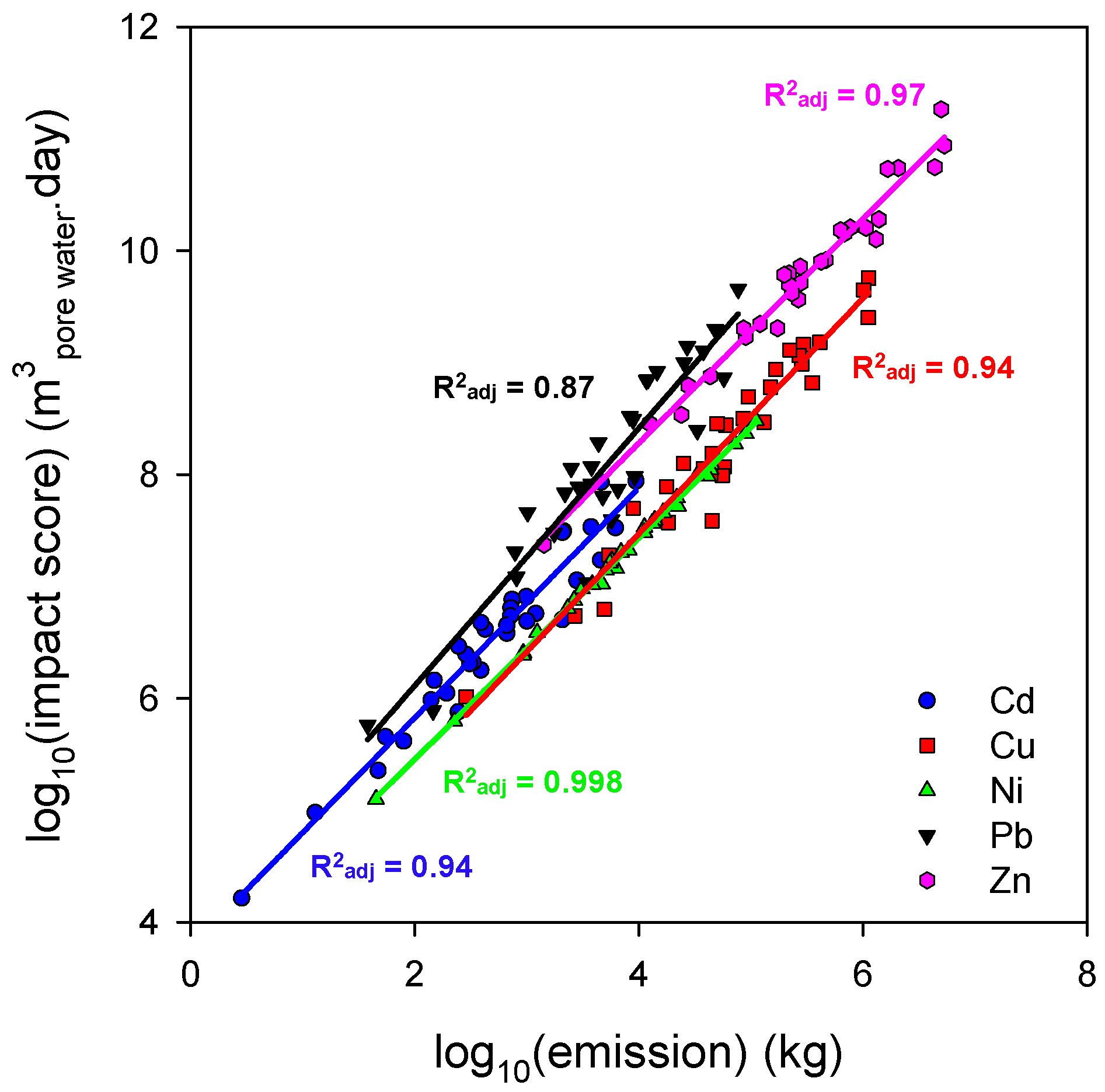
Appendix A.4. Prediction of Terrestrial Ecotoxicity Impact Scores

Table A9. Linear regression coefficients, adjusted R2 values (R2adj) and standard error of estimate (se) of regression equations for log10(ISs) of metal s (Cd, Cu, Ni, Pb or Zn). Emission of metal s (mtotal,s) is in kg, impact score (ISs) is in m3pore water·day. The regressions were developed by fitting a linear model to the data presented in Figure 4.
MetalRegressionnR2adjsep
Cd l o g 10 ( I S C d ) = 3.77 + 1.03 · l o g 10 ( m t o t a l , C d ) 330.940.2<2.2 × 10⁻¹⁶
Cu l o g 10 ( I S C u ) = 3.26 + 1.05 · l o g 10 ( m t o t a l , C u ) 300.940.21<2.2 × 10⁻¹⁶
Ni l o g 10 ( I S N i ) = 3.47 + 0.99 · l o g 10 ( m t o t a l , N i ) 300.9980.035<2.2 × 10⁻¹⁶
Pb l o g 10 ( I S P b ) = 3.81 + 1.15 · l o g 10 ( m t o t a l , P b ) 300.870.334.6 × 10−14
Zn l o g 10 ( I S Z n ) = 4.27 + 1 · l o g 10 ( m t o t a l , Z n ) 300.970.14<2.2 × 10⁻¹⁶

References

  1. Kumar, R.R.; Park, B.J.; Cho, J.Y. Application and environmental risks of livestock manure. J. Korean Soc. Appl. Biol. Chem. 2013, 56, 497–503. [Google Scholar] [CrossRef]
  2. Atafar, Z.; Mesdaghinia, A.; Nouri, J.; Homaee, M.; Yunesian, M.; Ahmadimoghaddam, M.; Mahvi, A.H. Effect of fertilizer application on soil heavy metal concentration. Environ. Monit. Assess. 2010. [Google Scholar] [CrossRef] [PubMed]
  3. Kuczyński, T.; Dämmgen, U.; Webb, J.; Myczko, A. Emissions from European Agriculture; Wageningen Academic Pub: Wageningen, The Netherlands, 2005. [Google Scholar]
  4. FAOSTAT Manure Applied to Soil. Available online: http://faostat3.fao.org/download/G1/GU/E (accessed on 19 June 2016).
  5. Provolo, G.; Manuli, G.; Finzi, A.; Lucchini, G.; Riva, E.; Sacchi, G.A. Effect of pig and cattle slurry application on heavy metal composition of maize grown on different soils. Sustainability 2018, 10, 2684. [Google Scholar] [CrossRef]
  6. Panagos, P.; Ballabio, C.; Lugato, E.; Jones, A.; Borrelli, P.; Scarpa, S.; Orgiazzi, A.; Montanarella, L. Potential sources of anthropogenic copper inputs to European agricultural soils. Sustainability 2018, 10, 2380. [Google Scholar] [CrossRef]
  7. Leclerc, A.; Laurent, A. Framework for estimating toxic releases from the application of manure on agricultural soil: National release inventories for heavy metals in 2000–2014. Sci. Total Environ. 2017, 590–591, 452–460. [Google Scholar] [CrossRef] [PubMed]
  8. Rosenbaum, R.K.; Bachmann, T.M.; Gold, L.S.; Huijbregts, M.A.J.; Jolliet, O.; Juraske, R.; Koehler, A.; Larsen, H.F.; MacLeod, M.; Margni, M.; et al. USEtox-the UNEP-SETAC toxicity model: Recommended characterisation factors for human toxicity and freshwater ecotoxicity in life cycle impact assessment. Int. J. Life Cycle Assess. 2008, 13, 532–546. [Google Scholar] [CrossRef]
  9. Hauschild, M.Z.; Huijbregts, M.A.J. Life Cycle Impact Assessment; LCA Compendium—The Complete World of Life Cycle Assessment; Springer: Dordrecht, The Netherlands, 2015; ISBN 9789401797443. [Google Scholar]
  10. Hauschild, M.Z. Assessing environmental impacts in a life-cycle perspective. Environ. Sci. Technol. 2005, 39, 81A–88A. [Google Scholar] [CrossRef] [PubMed]
  11. Owsianiak, M.; Rosenbaum, R.K.; Huijbregts, M.A.J.; Hauschild, M.Z. Addressing geographic variability in the comparative toxicity potential of copper and nickel in soils. Environ. Sci. Technol. 2013, 47, 3241–3250. [Google Scholar] [CrossRef] [PubMed]
  12. Pizzol, M.; Christensen, P.; Schmidt, J.; Thomsen, M. Eco-toxicological impact of “metals” on the aquatic and terrestrial ecosystem: A comparison between eight different methodologies for Life Cycle Impact Assessment (LCIA). J. Clean. Prod. 2011, 19, 687–698. [Google Scholar] [CrossRef]
  13. Owsianiak, M.; Holm, P.E.; Fantke, P.; Christiansen, K.S.; Borggaard, O.K.; Hauschild, M.Z. Assessing comparative terrestrial ecotoxicity of Cd, Co, Cu, Ni, Pb, and Zn: The influence of aging and emission source. Environ. Pollut. 2015, 206, 400–410. [Google Scholar] [CrossRef] [PubMed] [Green Version]
  14. Owsianiak, M.; Laurent, A.; Bjørn, A.; Hauschild, M.Z. IMPACT 2002+, ReCiPe 2008 and ILCD’s recommended practice for characterization modelling in life cycle impact assessment: A case study-based comparison. Int. J. Life Cycle Assess. 2014, 19. [Google Scholar] [CrossRef]
  15. Plouffe, G.; Bulle, C.; Deschênes, L. Characterization factors for zinc terrestrial ecotoxicity including speciation. Int. J. Life Cycle Assess. 2016, 21, 523–535. [Google Scholar] [CrossRef]
  16. Aziz, L.; Deschênes, L.; Karim, R.-A.; Patouillard, L.; Bulle, C. Including metal atmospheric fate and speciation in soils for terrestrial eco-toxicity in life cycle impact assessment. Int. J. Life Cycle Assess. 2017. Accepted. [Google Scholar]
  17. Santos, I.V.; Bulle, C.; Levasseur, A.; Deschênes, L. Regionalized terrestrial ecotoxicity assessment of copper-based fungicides applied in viticulture. Sustainbility 2018, 10, 2522. [Google Scholar] [CrossRef]
  18. Sydow, M.; Chrzanowski, Ł.; Cedergreen, N.; Owsianiak, M. Limitations of experiments performed in artificially made OECD standard soils for predicting cadmium, lead and zinc toxicity towards organisms living in natural soils. J. Environ. Manag. 2017, 198, 32–40. [Google Scholar] [CrossRef] [PubMed] [Green Version]
  19. Harmonized World Soil Database; Version 1.2; FAO/IIASA/ISRIC/ISS-CAS/JRC; FAO: Rome, Italy; IIASA: Laxenburg, Austria, 2012.
  20. Thenkabail, P.S.; Knox, J.W.; Ozdogan, M.; Gumma, M.K.; Congalton, R.G.; Wu, Z.; Milesi, C.; Finkral, A.; Marshall, M.; Mariotto, I.; et al. Assessing future risks to agricultural productivity, water resources and food security: How can remote sensing help? Photogramm. Eng. Remote Sens. 2012, 78, 773–782. [Google Scholar]
  21. Burton, C.; Martinez, J. Contrasting the management of livestock manures in Europe with the practice in Asia: What lessons can be learnt? Outlook Agric. 2008, 37, 195–201. [Google Scholar] [CrossRef]
  22. Araji, A.; Abdo, Z.; Joyse, P. Efficient use of animal manure on cropland-economic analysis. Bioresour. Technol. 2001, 79.2, 179–191. [Google Scholar] [CrossRef]
  23. Pickard, B.R.; Daniel, J.; Mehaffey, M.; Jackson, L.E.; Neale, A. EnviroAtlas: A new geospatial tool to foster ecosystem services science and resource management. Ecosyst. Serv. 2015, 14, 45–55. [Google Scholar] [CrossRef] [Green Version]
  24. Latham, J.; Cumani, R.; Rosati, I.; Bloise, M. FAO Global Land Cover (GLC-SHARE); Database Beta-Release Version 1.0; FAO: Rome, Italy, 2014; 40p. [Google Scholar]
  25. Owsianiak, M.; Huijbregts, M.; Hauschild, M.Z. Improved comparative toxicity potentials of 23 metallic elements in soils: Addressing solid- and liquid-phase speciation in environmental fate, exposure, and effects. In Proceedings of the SETAC Europe 27th Annual Meeeting, Brussels, Belgium, 7–11 May 2017. [Google Scholar]
  26. Pennington, D.W.; Payet, J.; Hauschild, M. Aquatic ecotoxicological indicators in life-cycle assessment. Environ. Toxicol. Chem. 2004, 23, 1796–1807. [Google Scholar] [CrossRef] [PubMed]
  27. Henderson, A.; Hauschild, M.; van de Meent, D.; Huijbregts, M.; Larsen, H.; Margni, M.; McKone, T.; Payet, J.; Rosenbaum, R.; Jolliet, O. USEtox fate and ecotoxicity factors for comparative assessment of toxic emissions in life cycle analysis: Sensitivity to key chemical properties. Int. J. Life Cycle Assess. 2011, 16, 701–709. [Google Scholar] [CrossRef]
  28. Fantke, P.; Bijster, M.; Guignard, C.; Hauschild, M.; Huijbregts, M.; Jolliet, O.; Kounina, A.; Magaud, V.; Margni, M.; McKone, T.; et al. USEtox®® 2.0; Documentation Version 1; USEtox® Team: Kgs. Lyngby, Denmark, 2017; ISBN 978-87-998335-0-4. [Google Scholar]
  29. Hauschild, M.Z.; Huijbregts, M.; Jolliet, O.; MacLeod, M.; Margni, M.; van de Meent, D.V; Rosenbaum, R.K.; McKone, T.E. Building a model based on scientific consensus for life cycle impact assessment of chemicals: The search for harmony and parsimony. Environ. Sci. Technol. 2008, 42, 7032–7037. [Google Scholar] [CrossRef] [PubMed]
  30. Heijungs, R. Harmonization of methods for impact assessment. Environ. Sci. Pollut. Res. Int. 1995, 2, 217–224. [Google Scholar] [CrossRef] [PubMed]
  31. Zhang, X.; Zeng, S.; Chen, S.; Ma, Y. Change of the extractability of cadmium added to different soils: Aging effect and modeling. Sustainbility 2018, 10, 885. [Google Scholar] [CrossRef]
  32. Zhang, A.; Cortes, V.; Phelps, B.; van Ryswyk, H.; Srebotnjak, T. Experimental analysis of soil and mandarin orange plants treated with heavy metals found in Oilfield-Produced wastewater. Sustainbility 2018, 10, 1493. [Google Scholar] [CrossRef]
  33. Fantke, P.; Aurisano, N.; Bare, J.; Backhaus, T.; Bulle, C.; Chapman, P.M.; De Zwart, D.; Dwyer, R.; Ernstoff, A.; Golsteijn, L.; et al. Toward Harmonizing Ecotoxicity Characterization in Life Cycle Impact Assessment. Environ. Toxicol. Chem. 2018. [Google Scholar] [CrossRef] [PubMed]
  34. Groenenberg, J.E.; Dijkstra, J.J.; Bonten, L.T.C.; de Vries, W.; Comans, R.N.J. Evaluation of the performance and limitations of empirical partition-relations and process based multisurface models to predict trace element solubility in soils. Environ. Pollut. 2012, 166, 98–107. [Google Scholar] [CrossRef] [PubMed]
  35. Kabata-Pendias, A.; Pendias, H. Trace Elements in Soils and Plants; CRC Press: Boca Raton, FL, USA, 2001. [Google Scholar]
  36. Groenenberg, J.E.; Römkens, P.F.A.M.; Comans, R.N.J.; Luster, J.; Pampura, T.; Shotbolt, L.; Tipping, E.; De Vries, W. Transfer functions for solid-solution partitioning of cadmium, copper, nickel, lead and zinc in soils: Derivation of relationships for free metal ion activities and validation with independent data. Eur. J. Soil Sci. 2010, 61, 58–73. [Google Scholar] [CrossRef]
  37. Thakali, S.; Allen, H.E.; Di Toro, D.M.; Ponizovsky, A.A.; Rooney, C.P.; Zhao, F.-J.; McGrath, S.P.; Criel, P.; Van Eeckhout, H.; Janssen, C.R.; et al. Terrestrial biotic ligand model. 2. Application to Ni and Cu toxicities to plants, invertebrates, and microbes in soil. Environ. Sci. Technol. 2006, 40, 7094–7100. [Google Scholar] [CrossRef] [PubMed]
  38. Szilágyi, A. Evaluation of Spatial Variability in the Comparative Toxicity Potential of Copper in Soils for Application in Life Cycle Assessment; University of Miskolc: Miskolc, Hungary, 2013. [Google Scholar]
  39. Smolders, E.; Oorts, K.; Lombi, E.; Schoeters, I.; Ma, Y.; Zrna, S.; McLaughlin, M.J. The Availability of Copper in Soils Historically Amended with Sewage Sludge, Manure, and Compost. J. Environ. Qual. 2012, 41, 506. [Google Scholar] [CrossRef] [PubMed] [Green Version]
  40. Thakali, S.; Allen, H.E.; Di Toro, D.M.; Ponizovsky, A.A.; Rooney, C.P.; Zhao, F.-J.; McGrath, S.P. A terrestrial biotic ligand model. 1. Development and application to Cu and Ni toxicities to barley root elongation in soils. Environ. Sci. Technol. 2006, 40, 7085–7093. [Google Scholar] [CrossRef] [PubMed]
  41. Leip, A.; Marchi, G.; Koeble, R.; Kempen, M.; Britz, W.; Li, C. Linking an economic model for European agriculture with a mechanistic model to estimate nitrogen and carbon losses from arable soils in Europe. Biogeosciences 2008. [Google Scholar] [CrossRef]
  42. Nakhone, L.N.; Young, S.D. The significance of (radio-) labile cadmium pools in soil. Environ. Pollut. 1993, 82, 73–77. [Google Scholar] [CrossRef]
  43. Sterckeman, T.; Carignan, J.; Srayeddin, I.; Baize, D.; Cloquet, C. Availability of soil cadmium using stable and radioactive isotope dilution. Geoderma 2009, 153, 372–378. [Google Scholar] [CrossRef]
  44. Ahnstrom, Z.A.S.; Parker, D.R. Cadmium reactivity in metal-contaminated soils using a coupled stable isotope dilution-sequential extraction procedure. Environ. Sci. Technol. 2001, 35, 121–126. [Google Scholar] [CrossRef] [PubMed]
  45. Huang, Z.Y.; Chen, T.; Yu, J.; Zeng, X.C.; Huang, Y.F. Labile Cd and Pb in vegetable-growing soils estimated with isotope dilution and chemical extractants. Geoderma 2011, 160, 400–407. [Google Scholar] [CrossRef]
  46. Ayoub, A.S.; McGaw, B.A.; Shand, C.A.; Midwood, A.J. Phytoavailability of Cd and Zn in soil estimated by stable isotope exchange and chemical extraction. Plant Soil 2003, 252, 291–300. [Google Scholar] [CrossRef]
  47. Gray, C.W.; McLaren, R.G.; Günther, D.; Sinaj, S. An Assessment of Cadmium Availability in Cadmium-Contaminated Soils using Isotope Exchange Kinetics. Soil Sci. Soc. Am. J. 2004, 68, 1210. [Google Scholar] [CrossRef] [Green Version]
  48. Stanhope, K.G.; Young, S.D.; Hutchinson, J.J.; Kamath, R. Use of isotopic dilution techniques to assess the mobilization of nonlabile Cd by chelating agents in phytoremediation. Environ. Sci. Technol. 2000, 34, 4123–4127. [Google Scholar] [CrossRef]
  49. Gray, C.W.; McLaren, R.G.; Shiowatana, J. The determination of labile cadmium in some biosolids-amended soils by isotope dilution plasma mass spectrometry. Aust. J. Soil Res. 2003, 41, 589–597. [Google Scholar] [CrossRef]
  50. Biasioli, M.; Kirby, J.K.; Hettiarachchi, G.M.; Ajmone-Marsan, F.; McLaughlin, M.J. Copper lability in soils subjected to intermittent submergence. J. Environ. Qual. 2007, 39, 2047–2053. [Google Scholar] [CrossRef]
  51. Nolan, A.L.; Ma, Y.; Lombi, E.; McLaughlin, M.J. Measurement of labile Cu in soil using stable isotope dilution and isotope ratio analysis by ICP-MS. Anal. Bioanal. Chem. 2004, 380, 789–797. [Google Scholar] [CrossRef] [PubMed] [Green Version]
  52. Sivry, Y.; Riotte, J.; Sappin-Didier, V.; Munoz, M.; Redon, P.O.; Denaix, L.; Dupre, B. Multielementary (Cd, Cu, Pb, Zn, Ni) Stable Isotopic Exchange Kinetic (SIEK) Method to Characterize Polymetallic Contaminations. Environ. Sci. Technol. 2011, 45, 6247–6253. [Google Scholar] [CrossRef] [PubMed]
  53. Nolan, A.L.; Ma, Y.B.; Lombi, E.; McLaughlin, M.J. Speciation and Isotopic Exchangeability of Nickel in Soil Solution. J. Environ. Qual. 2009, 38, 485–492. [Google Scholar] [CrossRef] [PubMed]
  54. Massoura, S.T.; Echevarria, G.; Becquer, T.; Ghanbaja, J.; Leclere-Cessac, E.; Morel, J.L. Control of nickel availability by nickel bearing minerals in natural and anthropogenic soils. Geoderma 2006, 136, 28–37. [Google Scholar] [CrossRef]
  55. Atkinson, N.R.; Bailey, E.H.; Tye, A.M.; Breward, N.; Young, S.D. Fractionation of lead in soil by isotopic dilution and sequential extraction. Environ. Chem. 2011, 8, 493–500. [Google Scholar] [CrossRef] [Green Version]
  56. Sanders, J.R.; El Kherbawy, M.I. The effect of pH on zinc adsorption equilibria and exchangeable zinc pools in soils. Environ. Pollut. 1987, 44, 165–176. [Google Scholar] [CrossRef]
  57. Diesing, W.E.; Sinaj, S.; Sarret, G.; Manceau, A.; Flura, T.; Demaria, P.; Siegenthaler, A.; Sappin-Didier, V.; Frossard, E. Zinc speciation and isotopic exchangeability in soils polluted with heavy metals. Eur. J. Soil Sci. 2008, 59, 716–729. [Google Scholar] [CrossRef] [Green Version]
Figure 1. Schematic overview of major methodological steps in the study using the example of Albania. Section 2.4. explains calculation of grid-specific CTPs,i using Equation (3). HWSD: Harmonized World Soil Database [19].
Sustainability 10 04094 g001
Figure 2. Comparative toxicity potentials (log10-transformed) of Cd, Cu, Ni, Pb and Zn across all 1 × 1 km grid cells in Europe.
Sustainability 10 04094 g002
Figure 3. Terrestrial ecotoxicity impact scores as function of the contribution of each country to total emissions of a metal and country-specific CTPs derived from grid-specific CTPi,s values, in m3pore water·day/kgtotal emitted to soil (Equation (2)). The country-specific impact scores are proportional to the area of each bar in the figures (Equation (3)), and the sum of all areas represents the total impact score in Europe for 30 (Cd) or 33 (Cu, Ni, Pb and Zn) countries. Country codes within the largest bars emphasize top contributing countries based on emissions. Values in brackets indicate the ranking based on impact scores. ESP: Spain; FRA: France; DEU: Germany; POL: Poland; NLD: The Netherlands; ROU: Romania; IRL: Ireland; ITA: Italy; DNK: Denmark; BLR: Belarus.
Sustainability 10 04094 g003
Figure 4. Terrestrial ecotoxicity impact scores (IS, in m3pore water·day) plotted against total emission of a metal (in kg) in European countries. Both the impact score and the total emission are log10-transformed. Color lines and (R2adj) represent linear regression fits to the data and their corresponding adjusted R2 values. The regressions are reported in Table A9.
Sustainability 10 04094 g004
Table 1. Summary of approaches used to calculate parameters and factors underlying the CTPs of the metals included in this study.
ParameterEquationUnitSource
Grid-specific distribution coefficient between total metal in the solid phase and total dissolved metal a
  K d , total s , i = s total , s , i c total   dissolved ,   s ,   i K d , reactive s , i ACF s  
Lpore water/kgsolidTotal dissolved concentrations were calculated using empirical regression models of Groenenberg et al. [34] from total metal concentration and soil properties. Reactive concentrations and reactive fraction were derived for metals from organic-related emission sources (including manures) in a meta-analysis study of Owsianiak et al. [13]. Background total metal concentrations are from Kabatia-Pendias [35]
Grid-specific distribution coefficient between reactive metal in the solid phase and total dissolved metal a
  K d , reactive s , i = s reactive , s , i c total   dissolved ,   s ,   i f reactive , s · C total , i , s  
Lpore water/kgsolid
Grid-specific fate factor in agricultural soil for emission to agricultural soil b
  FF i , s = Δ C total , s · V · ρ b Δ M i , s  
kgtotal/kgtotal emitted to soil·dayCalculated using USEtox 2.02 [28] for infinite time horizon
Spatially generic, emission-source specific accessibility factor in agricultural soil c ACF s = 0 T f reactive ,   s ( t ) dt T Δ C reactive ,   s Δ C total , s kgreactive/kgtotalDerived by Owsianiak et al. [13]. Because the influence of aging time on freactive,s was not consistent for five cationic metals, time-horizon independent ACFs are used. They are in practice equal to (time-independent) metal- and emission-source specific reactive fraction [13]
Grid-specific bioavailability factor in agricultural soil d
  BF s = Δ C free , s · θ w Δ C reactive , s · ρ b  
kgfree/kgreactiveFree ion concentrations were calculated from reactive concentration and soil properties using empirical regression models developed by Groenenberg et al. [36]
Grid-specific effect factor in agricultural soil e
  EF s = Δ PAF Δ C free , s = 0.5 HC 50 s  
m3pore water/kgfreeDerived using free-ion-based EC50 values using the approach of USEtox 2.02 [28]. The EC50 values were calculated using empirical regression models (Cd, Zn) and free ion activity models (Pb) developed for terrestrial earthworms and crustacea by Sydow et al. [18], and terrestrial biotic ligand models developed for various terrestrial organisms (Cu and Ni) by Thakali et al. [37]
a stotal,s,i (kgtotal/kgsolid) and sreactive,s,i (kgreactive/kgsolid) are the concentrations of total metal and reactive metal s in the solid phase in grid cell i; ctotal dissolved (kgtotal dissolved/Lpore water) is the concentration of total dissolved metal (assumed reactive) in soil pore water; Ctotal,s,i (kgtotal/kgtotal emitted) is the concentration of total metal s in soil in grid cell i; freactive,s, in kgreactive/kgtotal, represents the fraction of total metal s in soil that is available for solid-liquid partitioning within a time scale of days. b ΔCtotal,s,i (kgtotal/kgtotal emitted) is the incremental change in concentration of total metal s in soil in grid cell i; ΔMs,i (kgtotal emitted/day) is the incremental change in the emission of total metal s to soil in grid cell i; V (m3soil) is the volume of the soil compartment; and ρb (kgsoil/m3soil) is the total (wet) bulk density of soil. c freactive,s(t), in kgreactive/kgtotal, represents the fraction of total metal s in soil that is available for solid-liquid partitioning within a time scale of days as it varies with the aging time t (in years) of the metal in the soil (referred to as the reactive fraction); ΔCreactive,s (kgreactive/kgsolid) and ΔCtotal,s (kgtotal/kgsolid) are the incremental changes of the concentrations of reactive metal s and total metal in soil and T is the chosen time-horizon, in years. d ΔCfree,s,i (kgfree/m3pore water) is the incremental change of the free ion concentration of metal s in grid cell i; θw (m3pore water/m3soil) is the volumetric soil water content. e ΔPAF (dimensionless) is the incremental change in the potentially affected fraction of biological species in the soil ecosystem due to exposure to the free ion; and HC50s (kgfree/m3pore water) is the hazardous free ion concentration of metal s in grid cell i affecting 50% of the species, calculated as a geometric mean of (free-ion) EC50 values for individual species assuming a linear dose-response function. It is assumed that each grid cell i has the same species composition and density.
Table 2. Ranking of European countries according to their contributions to emitted mass and contributions to terrestrial ecotoxicity impact in those European countries for which impact scores could be calculated using Equation (1) and which contribute >1% of total emission. 100% is the total emission or total impact score (per metal) summed across all these countries. Hence the distribution of countries does not reflect the true distribution of emissions or impacts in entire Europe, and the contribution in the table should not be understood as a share of total European emissions or impacts. The number of countries considered for emissions and impacts is the same for each metal, thus making the country distributions comparable at metal level. Comparison can be done between the metals Cu, Ni, Pb and Zn, as the same countries were considered for these metals. All emissions and resulting impact scores are presented in Table A1 (Appendix A.1). ISO country codes are explained in Table A2 (Appendix A.1).
Country Contribution (in %)
CdCuNiPbZn
Emitted Mass of Metal (in kg)Impact Score (in m3pore water·Day)Emitted Mass of Metal (in kg)Impact Score (in m3pore water·Day)Emitted Mass of Metal (in kg)Impact Score (in m3pore water·Day)Emitted Mass of Metal (in kg)Impact Score (in m3pore water·Day)Emitted Mass of Metal (in kg)Impact Score (in m3pore water·Day)
FRA19.9FRA21.5DEU18.1DEU23.9DEU18.5DEU18.9DEU18.2DEU29.4DEU18.5ESP30.1
DEU13ESP20.9ESP18POL18.7ESP17.3ESP14.5ESP13.5POL12.9ESP17.3DEU14.3
ESP9.7ITA8.3POL16.3ESP10.6POL15.1POL11.7POL11.3NLD9.1POL15.1POL9.1
POL9.5DEU8.2NLD6.7NLD6.4IRL4.8IRL7.6IRL8.9IRL8.2NLD7.2NLD9
ITA7.9NLD7.7ROU5.7DNK6.1ROU5.8ROU6.9ROU7.8BLR6.5ROU5.8ROU8.8
IRL5.9ROU7.5DNK4.8BEL5.4NLD7.2NLD6NLD6.4BEL5.4IRL4.8IRL3.1
NLD4.5POL4.2IRL4.6BLR4.9BLR4.5BLR6BLR6ESP4.8DNK4.8DNK3.1
ROU4.4IRL2.8BLR4.4IRL4.1DNK4.8BEL3.9BEL3.4AUT4.6BLR4.5AUT2.6
BLR4.4AUT2BEL3.6AUT3.6BEL3.7DNK3.2AUT2.8DNK4.5BEL3.7BEL2.6
BEL2.5GRC1.9AUT2.7ROU2.8AUT2.7AUT2.8DNK2.8CZE2.1AUT2.7HUN2.5
DNK2.1HUN1.6SRB2.4SRB2.5HUN2.2HUN2.4HUN2.2CHE2SRB2.4SRB2.3
AUT2.1BEL1.4HUN2.1CZE2.1SRB2.4SRB2.3SRB2.1SRB2HUN2.2BLR2.1
GRC1.6SRB1.3CZE1.5CHE1.3CZE1.6CZE2.1CHE2.1ROU1.6CZE1.6CZE1.3
HUN1.5BLR1.2CHE1.4HUN1.2CHE1.5CHE1.9CZE2BIH1.3CHE1.5CHE1.3
SRB1.5DNK1.2 BIH1.2 BGR1.3BGR1.5 BGR1.2
CZE1.4ALB1.2 HRV1.2 ALB1.3ALB1.3
CHE1.4CHE1.1 BIH1.1LTU1.1

