1. Introduction
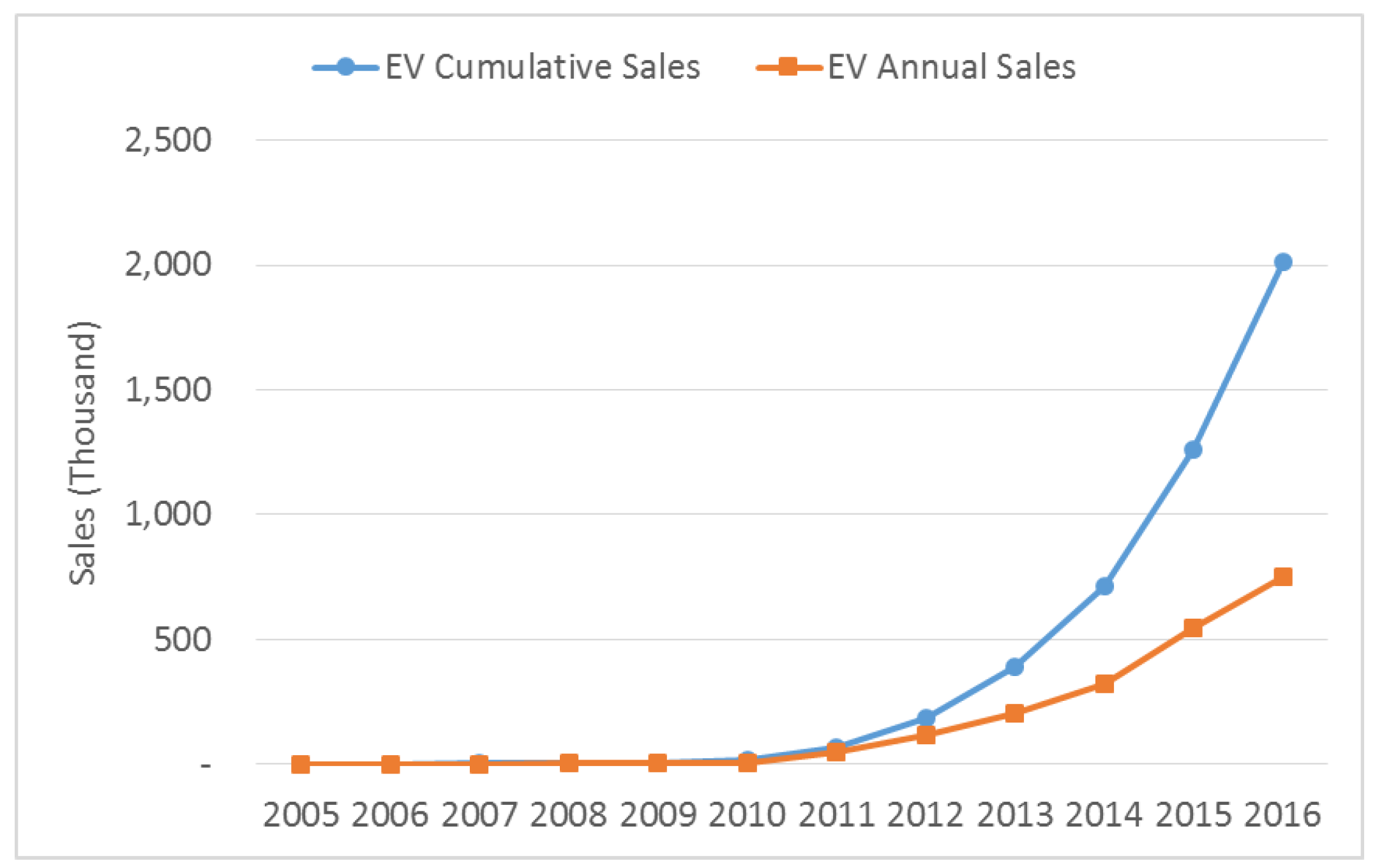
With recent rapid increases of electric vehicle (EV) demand, the amount of global cumulative sales exceeded two-million mark in 2016, and it does not show the signs of slowing down as shown in
Figure 1. The U.S. Energy Information Administration (EIA) estimated that projected cumulative sales and annual sales of EV in 2025 will be approximately 55 million and eight-million, respectively, based on 10 major EV manufacturer’s target sales. The reason of this significant sales increase is because the price of EV is rapidly approaching that of conventional vehicle, which is mainly caused by a significant decrease in the price of Lithium-Ion Battery (LIB) pack. The price of LIB pack dropped down to one-fifth level in seven years from approximately
$1000/kWh in 2010 to
$209/kWh in 2017, and it is expected to decrease below
$100/kWh by 2025 [
1]. This cost of LIB pack fall makes EV price competitive level to conventional vehicle and it brings the tipping point of active spread of EVs sooner [
2,
3].
With this soaring EV sales, on the other hand, the concern arises regarding the supply of LIB.
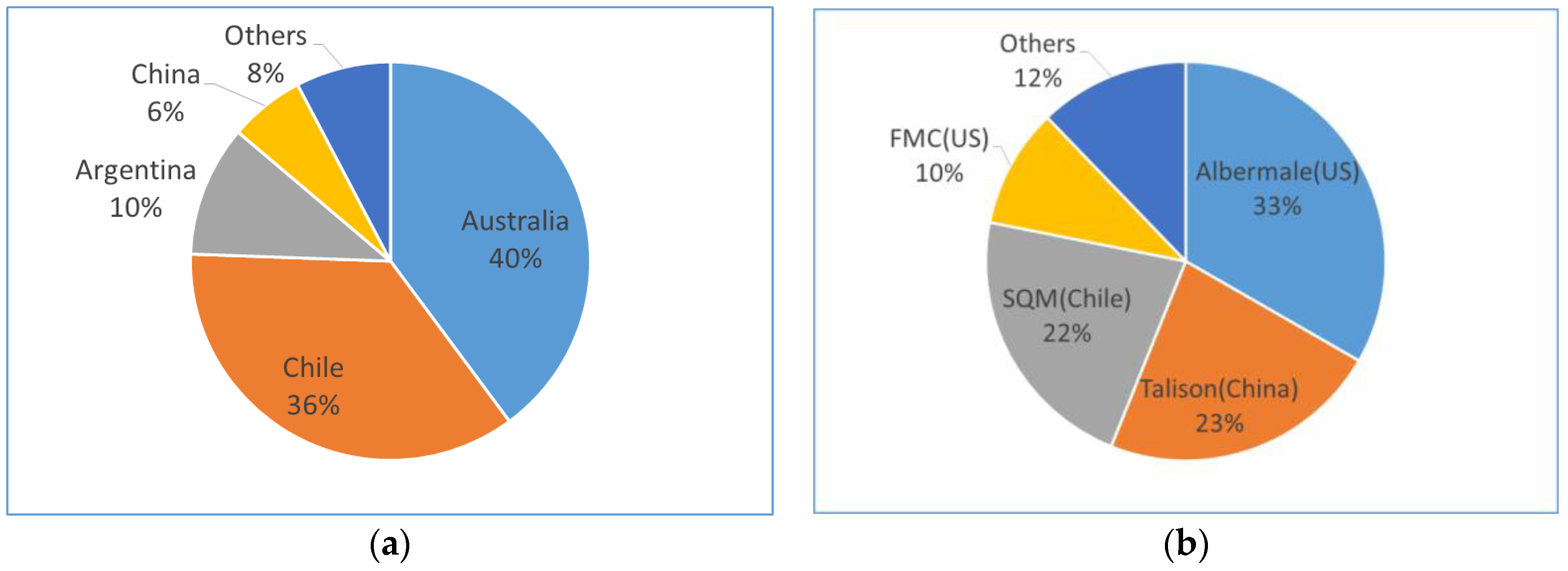
Table 1 shows that LIB, which can be classified as rechargeable battery, is the most dominant end-use type among all end-use of lithium, which takes approximately 37%. This proportion is projected to further increase as the EV sales rise, which leads to a significant rise of global lithium demand. However, the supply increase needed to support expected demand rise is not very optimistic because of its oligopolistic market characteristics, as shown in
Figure 2. 92% of global lithium mining is from four countries, such as Australia, Chile, Argentina, and China, and also 88% of lithium is supplied by four companies. Hence, a limited number of suppliers have market power in the global lithium market and this vulnerability in the lithium supply is a potential risk to achieve continuing LIB price drop, which is a key driver for active deployment of EVs. In addition,
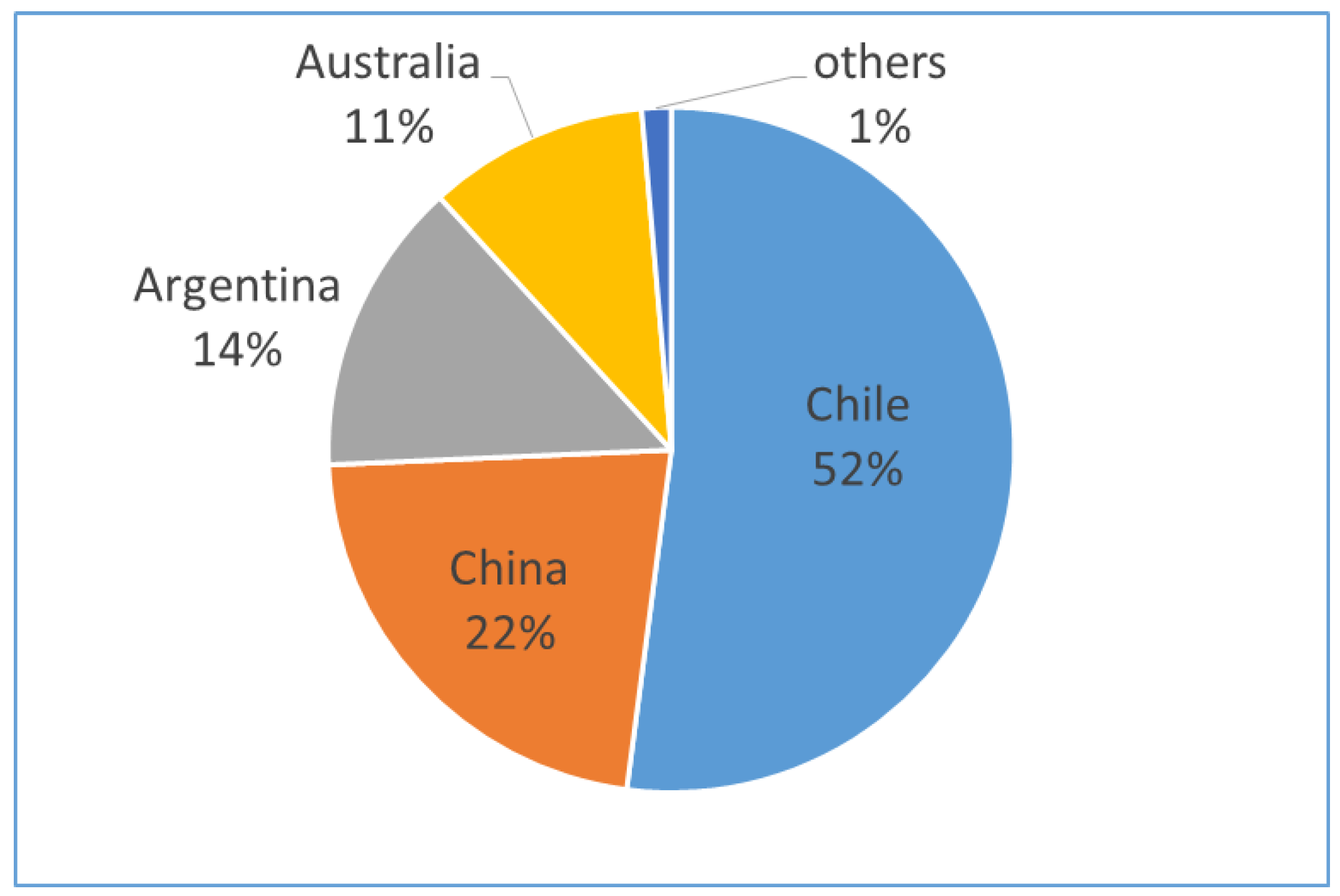
Figure 3 shows composition of lithium reserve by countries. Chile has more than 50% of world lithium reserve and China has 22% of total reserve.
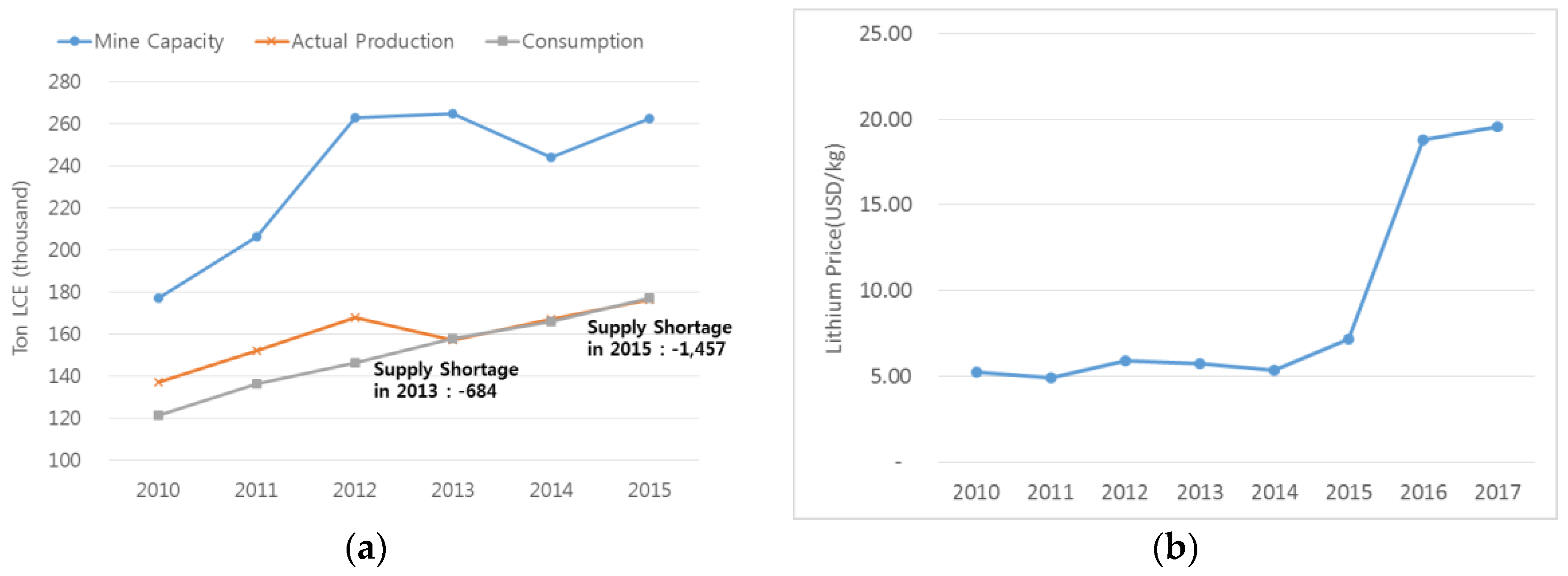
The impact of oligopolistic power in the lithium price can be confirmed in
Figure 4. Lithium production had been steadily larger than market demand until 2012, which means that supply has been sufficiently supporting demand. However, sudden supply shortage occurs in 2013, even though mine capacity was much larger than actual production level. In fact, the ratio of production to mine capacity in 2013 is the largest level in recent six years, which means that suppliers had abundant capacity to increase the production to meet soaring demand, but instead of increasing, they intentionally decreased lithium supply to boost up the price. Since 2013, the market consistently experienced supply shortage, and consequently as suppliers intended, the lithium price jumped up to almost four times from approximately
$5/kg in 2014 to
$20/kg in 2017. This is strong evidence supporting the idea that the recent LIB demand rise that is mainly caused by the increase of EV demand triggered suppliers to exercise the oligopolistic power and this has a significant impact on lithium prices. Hence, it would be meaningful to examine the dynamics between lithium and EV demand to forecast the future lithium price when EV demand continues growing as predicted.
In addition to lithium, there are three other materials required to manufacture LIB, which are cobalt, nickel, and manganese, and it is also important to understand the dynamics between these materials and EV demand to correctly forecast future material prices as prices of those other materials will also have a significant impact on the LIB cost. Hence, in this study, we examine the directional relationships between the prices of four main LIB metals and EV demand. In addition to conventional short-run estimation, this paper also analyzes the EV demand shock effect on cobalt, lithium, nickel, and manganese prices in the long run. We estimated the LIB metal prices using the VECM (Vector Error Correction Model) in order to analyze the dynamics of metal prices. EV demand is included as an exogenous variable in the VECM model to analyze the short-run and long-run impact on LIB metal prices.
In addition, we also examined the recycling effect of LIB materials on the future material price forecasting. In recent years, LIB recycling has been drawing a lot of attention as the volume of used LIB gradually increases. LIB recycling has two main advantages. The first one is an environmental advantage, as it can help in disposing old batteries in an environmental-friendly way. The second one is an economic advantage as materials in used LIB can be collected and reused, which will have a major impact on future LIB material prices, as collected materials are additional supply in the market. Assuming scenarios wherein lithium and cobalt were recycled in EV battery, we explored the impact of recycling policies on the material forecast price.
This paper is organized as follows.
Section 2 discusses extant literature on metal price estimation.
Section 3 describes the data and methodology. In
Section 4, we present the empirical results, while
Section 5 concludes the study.
2. Literature Review
Several studies focus on metal price movement in terms of price forecasting and price cycles. C. Ciner [
6] examines the long-run trend between the prices of gold and silver futures contracts traded on the Tokyo Commodity Exchange, based on cointegration tests. The study concludes that stable relationship between gold and silver prices disappeared in the 1990s. Thus, gold and silver markets should be approached as separate markets. Dooley et al. [
7] analyzes the future lead and zinc prices while using different time series forecasting method. Specifically, lagged forward price and ARIMA models were tested for their cash price forecasting power. According to the results of the paper, ARIMA price forecasts provide superior results when compared to lagged forward price models, in the case of lead price. Auer [
8] investigates precious metal markets focused on gold, silver, palladium, and platinum while using dummy-augmented GARCH models. This study confirms that there is significant evidence of time-varying skewness and kurtosis in precious metals returns.
Labys [
9] focuses on short-term price movements for aluminum, copper, gold, lead, nickel, silver, tin, tungsten, and zinc. This study uses the Weibull test of cyclical duration for discovered cycles and the structural time series method. The test results support existence of cyclical behavior in the expansion, contraction, and duration phases for a number of metal prices. On the other hand, Davutyan et al. [
10] claims that metal price movement is random, and the cyclicality of metal price is false for lead, zinc, mercury, tin, and copper prices. Rossen [
11] explores the long- and short-run cyclical behavior, and the respective co-movement of metal prices. This study examines the dynamics of 20 monthly price series of a variety of mineral commodities (copper, lead, tin, zinc, chromium, cobalt, manganese, etc.) in the last 100 years. It notes that metal prices increase more strongly in a shorter period than they fall, and they do not necessarily follow similar patterns.
From the macroeconomic point of view, Soytas et al. [
12] examine the long- and short-run transmissions of information between the world oil price, Turkish interest rate, Turkish lira–US dollar exchange rate, and domestic spot gold and silver price. They find that the world oil price did not have the predictive power of precious metal prices. In addition, transitory positive initial impacts of innovations in oil prices on gold and silver markets are observed. Sari et al. [
13] examines the co-movements and information transmission between the spot prices of four precious metals—gold, silver, platinum, and palladium—oil price, and the US dollar/euro exchange rate. It finds a weak long-run equilibrium relationship, but strong feedbacks, in the short run. In addition, there are evidence that spot precious metals’ prices and exchange rate are closely linked in the short run. Apergis et al. [
14] investigates the dynamics of precious metal prices in order to infer the information transmission that is based on FAVAR model. They confirm that the price transmission across precious metal markets, stock markets, and the macroeconomy is substantial. Methodology and variables analyzed for each literature are summarized in
Table 2.
In addition, literatures such as Freitas et al. [
15], Martin et al. [
16], Sadorsky [
17], Akram [
18] and Oh et al. [
19] analyzes causal relationship between various metal prices or energy consumption and macroeconomic data such as GDP, interest rate and exchange rate.
In the literatures that are summarized in
Table 2, four distinctive methodologies are used to analyze dynamics of various metal prices, which are Autoregressive Integrated Moving Average (ARIMA), Generalized Autoregressive Conditional Heteroscedasticity (GARCH), cyclical behavior model, and factor-augmented vector autoregressive (FAVAR). ARIMA is one of the time series data forecasting models that investigates the stochastic properties of the time series on its own as the basis for predicting future values of a variable. This model analyzes single dependent variable only and cannot analysis the vector of depend variables. GARCH is one approach to modeling time series with heteroscedastic errors. This model fits to analysis very volatile time series data and it is used widely in the financial market data analysis. The cyclical behavior approaches can be applied to test and forecast super long run cycles (at least 100 years) of variables, but this long term analysis cannot capture the recent changes and short term relations between variables. FAVAR can be used to avoid the degrees of freedom problem present in standard vector autoregression (VAR) models. However, FAVAR cannot be applied when the data have the long run relationship. In addition, this study uses VECM (Vector error correction model), which is basically time-series model and is used to investigate Granger causal relationships between variables when considering various time lags. Estimation results from the VECM analysis can show how one variable affects the movements of other variables in both short-run and long-run perspectives.
In this study, we analyzed the price movement and long-run dynamics of four metals (cobalt, lithium, manganese, and nickel) that are necessary to produce LIB. We selected EV demand as an exogenous variable to explain the movements of LIB metal prices, and explored its effect on the movement of lithium-ion battery material prices based on the VECM. We also evaluate the effect of the EV demand shock on the prices of major materials in lithium ion batteries, and lastly we estimate the impact of recycling of LIB on those prices of four metals.
3. Data and Methodology
The data used in this study consists of monthly time series of LIB material prices, such as lithium, cobalt, nickel, and manganese, and EV demand from 2008 to 2016. The variables are denoted P
cobalt, P
lithium, P
nickel, P
manganese, and EV demand, respectively. Nickel and cobalt prices were obtained from London Metal Exchange (LME), while lithium and manganese prices were obtained from Asian Metal. All the prices unit are converted to USD per ton. Descriptive statistics of these input data are provided in
Table 3.
The EV demand data are from the International Energy Agency [
4]. From the Global EV Outlook 2017 [
1], the new registrations of electric cars data are reported; we assumed that the EV battery capacity in 2008 was 18 KWh, and the efficiency of EV batteries improved by 4% per year. Based on new EV registration data and EV battery capacity assumption, we generated the EV battery demand (unit: MWh).
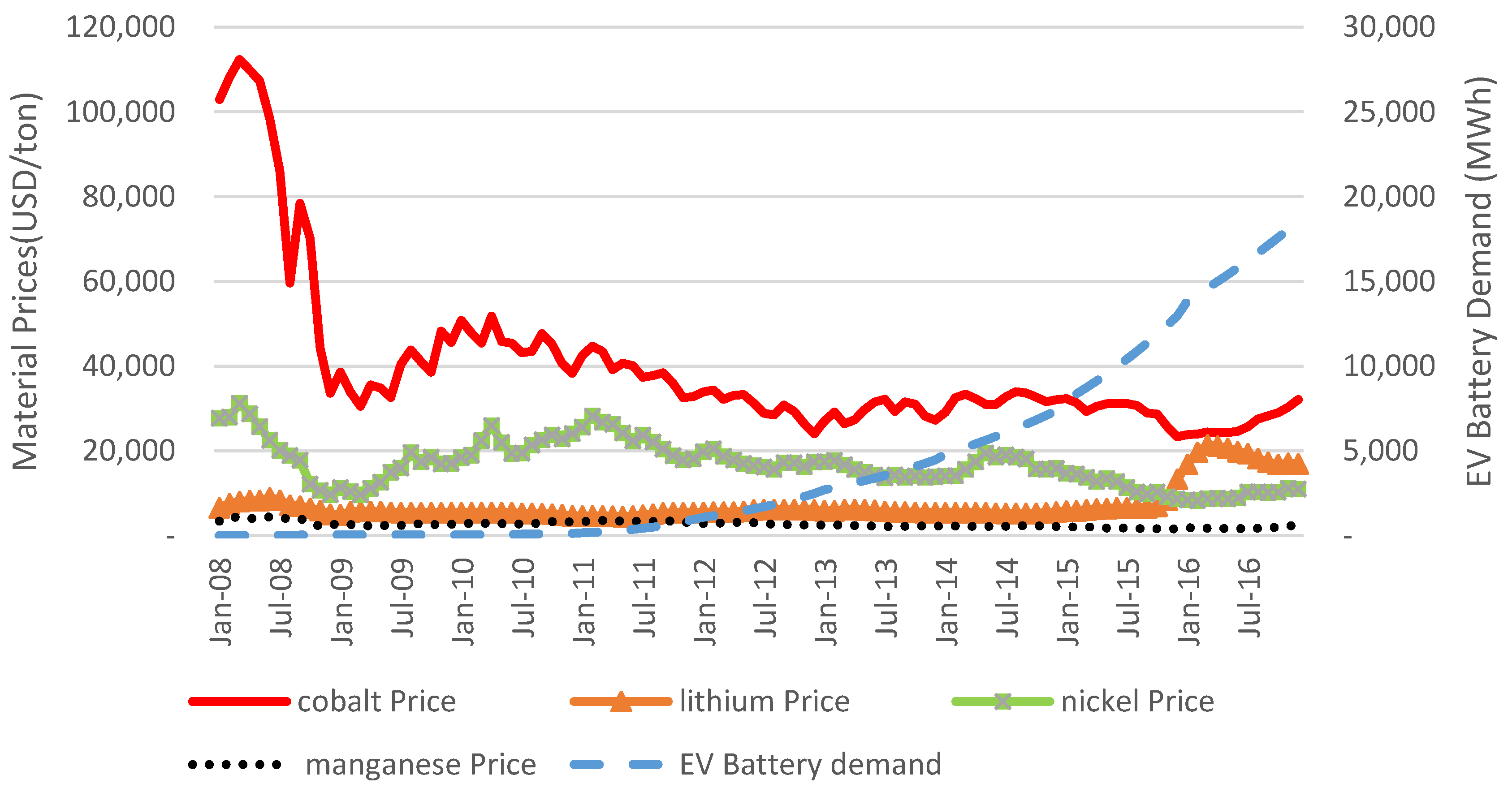
As per
Figure 5, the demand for EV batteries has been on the rise since 2014. Among metals, cobalt price has the highest volatility and mean. From 2015 onward, lithium and cobalt prices rapidly increased due to increase in metal demand in the downstream industry and supply shortage. However, it is not clear whether these metal price increases were due to demand growth or supply shortages. On the other hand, the price of manganese decrease over time, with less volatility than other raw metal prices.
The relatively high positive correlation between lithium price and EV demand is noted in
Table 4. This correlation indicates that lithium price and EV demand move closely in the same direction. On the other hand, other metal prices have a negative correlation with demand for EVs.
The objective of this study is to analyze the lithium-ion material prices movement and EV demand relationship with metal prices. We attempt to discover whether an increase in demand for EVs actually leads to a rise in metal prices. To examine the relationship between variables, time-series data analysis is applied. If the data have a unit root, a spurious regression problem may occur. To confirm the stability of each variable, unit root test is performed. If the data are not stable, a cointegration test will be performed to test the long-term relationship between variables. Finally, using the VECM method, we analyze the relationship between EV demand and metal prices.
4. Empirical Results
4.1. Unit Root Test Result
Before testing for the presence of cointegration, we use the Augmented Dickey–Fuller [
20], Pillips-Perron [
21], and Kwiatkowski et al. (KPSS) [
22] methods to test for the existence of unit roots, and to identify the order of integrations for each variable. Unit root tests are done with and without time trend, and the results are reported in
Table 5. The consistent suggestions of all these test results are that a unit root test can be rejected for the first difference, but not the levels for all metal prices data at the 5% significance level, except EV demand data. Thus, the unit root results imply that the metal price data is not stationary, but price changes move in a stationary pattern.
4.2. Cointegration Result
To test the existence of long-run equilibrium relationship between LIB raw metal prices, the Johansen [
23] cointegration test is performed. Even though the metal prices are not stationary, it is possible for a stationary linear combination to exist, which makes the cointegration relationship between metal prices. Therefore, we executed a Johansen cointegration test with a unit root test.
p’th order VECM, with exogenous variables using the cointegration test is adopted, as shown in Equation (1), below.
is a (1 × 4) vector of prices measured at time t: is the price of cobalt, is the price of lithium, is the price of manganese. ∆ is the first order difference operator, α is the matrix with the estimations on the speed of adjustment to the equilibrium, β is the cointegrating vectors, is a matrix with the estimations of short-run parameters relating price changes lagged i periods, is a coefficient associated with the EV demand that represents the exogenous variable, and is white noise.
By examining the matrix, we detect the existence of cointegrating relations among the LIB material prices. The rank (, r, can be tested with two statistics, such as trace test and maximum eigenvalue test, where the null hypothesis is r = g co-integrating vectors against the alternative hypothesis that r g + 1.
Based on several criteria, such as LR (Likelihood Ratio) test, Akaike’s Information criterion (AIC), FPF (Final prediction error), Hannan-Quinn Information criterion (HQIC), and Schwarz Information criterion (SC), we determine the optimal lag length (k) for the VAR in levels, as shown in
Table 6. SC and HQ indicate that the optimal lag length is 2. On the other hand, LR test, FPF, and AIC employ the optimal lag length as 4. Finally, we decide to use 4 for k. In our model, the Johannsen [
23] asymptotic critical values are no longer valid, because of the EV demand used as an exogenous variable to explain LIB metal prices. Therefore, we use the asymptotic critical values that are provided in Mackinnon et al. [
24]. From
Table 7, we conclude that there is one cointegration vector at a 5% significant level, because the trace and maximum eigenvalue tests reject the null hypothesis of zero cointegration rank. Since the cointegration vector exits, we use the VECM to analyze the lithium-ion metal price movement.
4.3. Estimation of VECM
With the cointegration rank and the optimum number of lags determined, the parameters of the VECM can be estimated. It is assumed that the prices of all LIB metals are influenced by the demand of EVs, which is the upstream metal industry. On the other hand, the demand of EVs is not influenced by metal price. Therefore, we constructed a VECM with four metal prices as the main variables, and used the EV demand as an exogenous variable of the VECM. The results are reported in
Table 8.
From the cointegrated vector (β), which is the normalized price of cobalt, we find that, in the long-run equilibrium, the rise of lithium and nickel prices decreases cobalt price. As the price of lithium and nickel rises, the price of LIB rises; eventually, the demand for cobalt decreases due to the decline in final demand. On the other hand, a one US dollar increase in manganese price increases cobalt price by 17 US dollar. This is because the roles of manganese and cobalt are similar in the functioning of the metal in the LIB. In the case of manganese, similar to cobalt, an increase in the ratio of the cathode material, functions to increase the battery stability. Therefore, if the manganese prices increase, the demand for manganese is substituted by cobalt demand, resulting in a rise in cobalt prices in the long run. In addition, under the 1% significant level, only the adjustment coefficient of cobalt price rejects the null, thus long-run relationships are important for cobalt prices.
In case of the exogenous variable, we attempt to confirm that the EV demand is important for short run dynamics of cobalt and lithium prices. This means that the EV demand strongly affects cobalt and lithium price changes in the short run. We may thus conclude that the surge in cobalt and lithium prices, which have been recorded since 2015, was caused by the recent explosive increase in demand for EVs, rather than supply shortages. On the other hand, demand for EVs did not have a statistically significant effect on the manganese and nickel price changes.
Lastly, we conduct a residual analysis for model diagnostic testing. The results are reported in
Table 9. Although serial correlation does not exist, autoregressive conditional heteroscedasticity and non-normality exist in the residuals. However, from the residuals correlation matrix in
Table 10, we conclude that the correlation among all residuals is very low, and this is not likely to be a major problem.
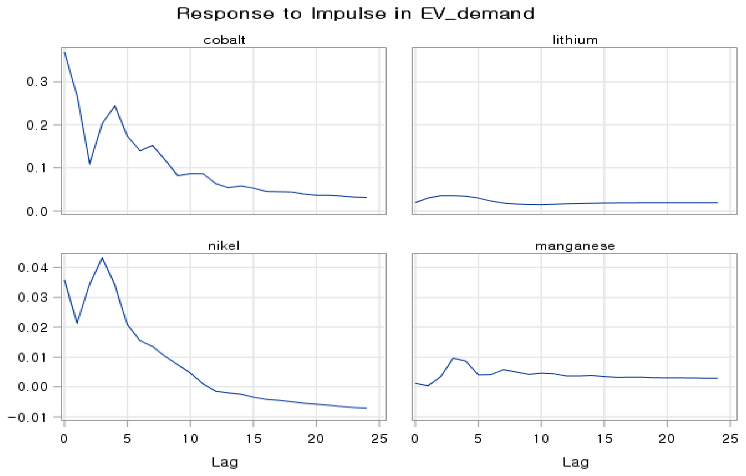
Figure 6 shows the responses of cobalt, lithium, nickel, and manganese prices to a forecast error impulse in EV demand. It is possible to observe that this demand has an immediate positive effect on cobalt price; the effect peaks during first month and it remains positive for over two years. For nickel price, the shock of demand for electric cars is approximately ten times lower than that of cobalt; the shocks remain positive until one year, and then, changed to negative. On the other hand, the EV demand shock to lithium and manganese prices is relatively small; it is positive for over two years. In conclusion, cobalt prices are the most sensitive to impact of changes in EV demand among secondary battery material prices, and the effect is maintained for the longest duration.
4.4. Recycling Effect on Material Price Forecasts
Along with the explosive increase in battery demand, the recycling of battery materials has also gained significant attention. Recycling can be beneficial for two reasons. Firstly, it can dispose old batteries in an environmentally friendly way; many hazardous parts can be reused, too. Secondly, it is economically beneficial, because valuable battery materials can be collected in the process of recycling. Hence, in this section, we analyze how the forecasts of cobalt and lithium prices, from 2017 to 2027, can be influenced by material recycling policy.
For recycling scenarios as shown in
Table 11, we assumed that a portion of battery demand of EV at time t will replace EV battery demand at t + 9, assuming that average battery replacement time period for EV is approximately nine years (The rationale for this average battery replacement period is that Tesla provides battery warranty for either eight years or 160,000 km for standard range battery, and Average driving distance of suburb area per day in U.S. is approximately 46.1 km/day according to DOE [
25]. This means that it takes approximately 9.5 years to reach 160,000 km. In addition, Tesla offers a battery replacement program in eight years for the upfront payment of
$12,000. Based on this information, average battery replacement period is selected as nine years). For instance, if 10% of EV battery produced in 2010 are recycled in 2019, it will reduce the demand for EV battery materials in 2019. This is because net EV battery demand, which is base demand in 2019, minus demand replaced by recycled materials from 2010, will be actual battery demand that requires newly produced metal materials from mines. To see the effect of different recycling ratios, 10%, 30%, and 50% scenarios are tested.
Based on the three scenarios, the effects of lithium and cobalt price forecasting changes on different material recycling policies are calculated. The EV demand forecasts used to forecast metal price is from BNEF [
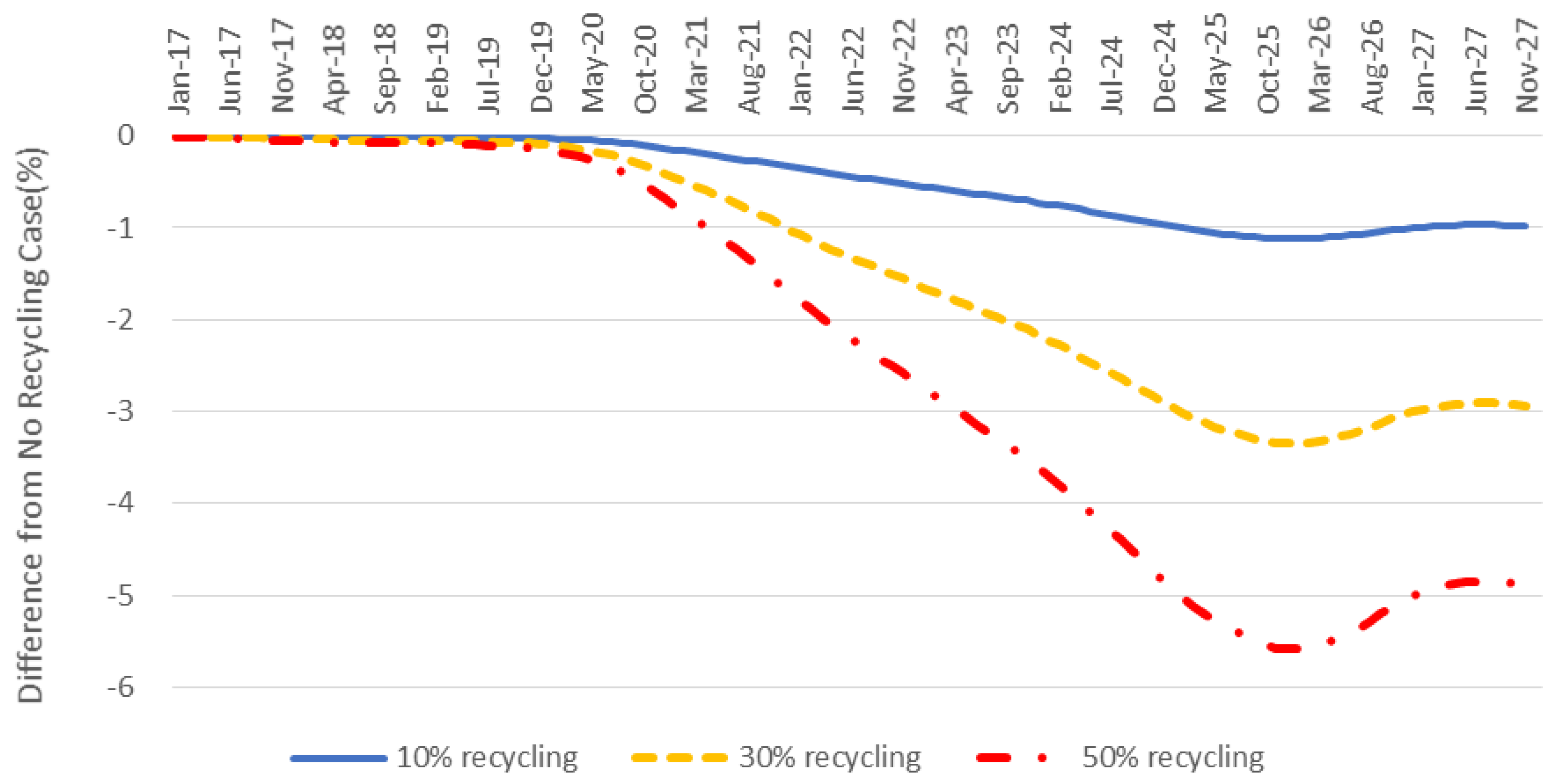
1]. As can be seen in
Figure 7, when we adopt the EV battery recycling policy, the price of cobalt material dropped notably. In particular, if 10%, 30%, and 50% of cobalt are recycled from EV batteries, the forecasted price will fall 1.0%, 3.1%, and 5.1% when compared to non-recycling case, respectively. Cobalt’s price volatility will also decrease according to the material recycling policy; the standard deviation of the cobalt price forecasting for the next 10 years will be 0.8%, 2.4%, and 4.0% lower than the non-recycling case.
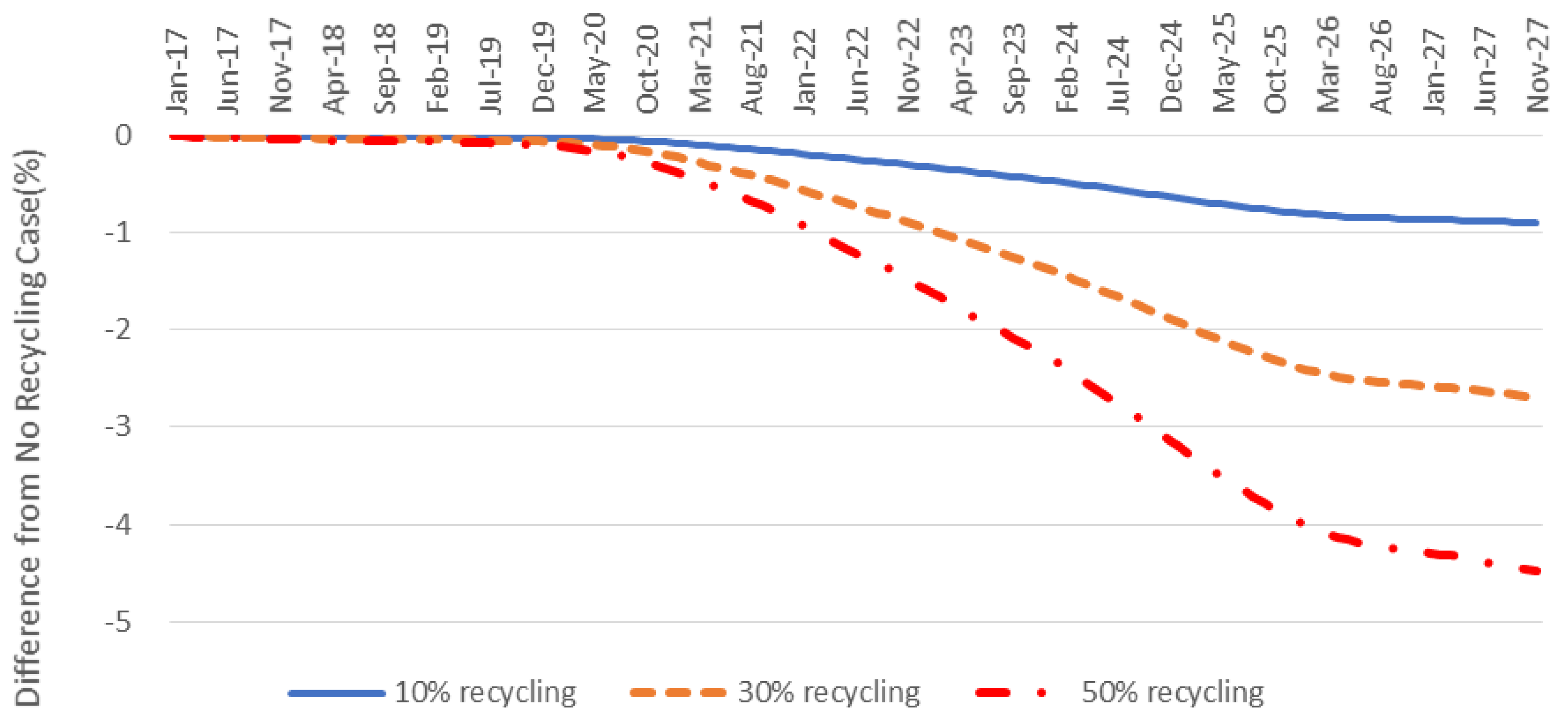
In the case of lithium recycling, similar policy effect as a cobalt case appears, and the price reduction is slightly less than that of cobalt. From
Figure 8, we conclude that, if we recycle 10%, 30%, and 50% of the lithium material from the electric car battery, the forecasted lithium price will decrease by 0.8%, 2.5%, and 4.1% when compared to the non-recycling case, respectively. The price volatility of lithium also decreases with the material recycling policy, and the standard deviation of the lithium price forecast for the next 10 years will be 0.6%, 1.9%, and 3.2% lower.
5. Discussion and Conclusions
The prices of major materials for lithium-ion batteries, such as lithium and cobalt, have been rising sharply in recent years. Cobalt prices have increased significantly—from an average of US$23,348 per ton in December 2015 to US$32,136 per ton in December 2016, with an annual average growth rate of 37.6%. More recently, cobalt prices increased even more sharply to US$72,589 per ton in December 2017 and 81,969 per ton in June 2018, which is 134% annual growth rate in this period. The price of lithium increased from US$13,324 per ton in December 2015 to US$16,950 per ton in December 2016, with an annual average growth rate of 27.2%, and recently, unlike cobalt, the lithium price is stationary as it is US$22,914 per ton in December 2017 and $16,582 per ton in Jun 2018. This surge in raw material prices is largely due to the increasing demand for rechargeable batteries, brought on by the growth in the electric car market. In particular, with the development of high-capacity batteries, the amount of raw materials used has been increasing. Therefore, it is important to estimate the prices of major materials for lithium-ion batteries, as their demand is expected to continue growing.
The main objective of this study is to investigate the dynamics of LIB raw material prices and the relationship between EV demand and LIB metal prices. The empirical results confirm that, in the long-run equilibrium, lithium and nickel prices move inversely with cobalt prices. If the prices of LIB materials, such as lithium and nickel, rise, the LIB price also increases, and this increase results in a further decline in cobalt demand, which, in turn, leads to a decline in cobalt prices.
Results of VECM estimation show that EV demand is important to short-run dynamics of cobalt and lithium price at a 5% significance level; that is, the demand for secondary batteries, mostly by EVs, has led to a sharp increase in the prices of lithium and cobalt. Moreover, the impulse response results show that EV demand has an immediate positive effect on cobalt price; the effect peaks during the first month and remains positive for over two years. On the other hand, the EV demand shock to nickel, lithium, and manganese prices is relatively small. Therefore, we confirm that cobalt prices are the most sensitive to the impact of changes in EV demand among secondary battery material prices, and the effect is maintained for the longest duration. We also analyze changes in cobalt and lithium price forecasts that are based on secondary battery material recycling policies. We found that, with strengthened material recycling policies, material prices reduced from 1% to 5%, and price volatility also reduced.
In addition to massive demand increase of EVs, the expansion of renewable generation in power systems will also increase the demand for energy storage installation because energy storage is effective to mitigate the inherent variability and intermittency of renewable sources. Hence, demand for mid- to large-sized LIB is expected to continue growing sharply. Results in this study show that EV demand is expected to drive up the prices of lithium and cobalt. Since these materials have limited supply due to its oligopolistic market structure, following two policies will help in lessening the supply shortage of LIB materials.
First, we must expand current policy regarding the development of LIB recycling technology. In Korea, while the secondary battery industry is well-developed, the material industry still has a very weak supply chain. Due to the absolute reliance on lithium, cobalt, and other raw material imports for cathodes, fluctuations in material prices have a negative effect on the entire secondary battery industry. Currently, Korea has developed a recycling technology for recovering valuable metals through the wet process only for medium-sized lithium-ion batteries. In future, it is necessary to develop a variety of new processes to enhance the economic efficiency of recycling wet processes that are related to recycling secondary batteries. We must also develop dry process technologies that do not have original technologies in Korea. In addition, it is necessary to find and execute R&D projects related to the performance and durability test of cathode materials while using recycled rare metals, and ESS performance tests using used electric batteries.
Second, it is necessary to develop (1) new materials to replace the main metal of lithium ion batteries; (2) cost-competitive new materials to replace expensive and highly volatile metals, like lithium and cobalt; and, (3) a secondary battery with higher performance, low cost, and high battery energy density by researching the content ratio of NCM (Nickel, Cobalt, and Manganese).
Lastly, in the near future, new technology may change the long-run equilibrium relationship among metal prices that this study estimated. High demand for LIB will trigger a sharp increase in related metal prices and if this continues, technology or market will find alternatives. One technology that is under R&D is to change the proportion of chemistry among Nickel, manganese and cobalt (NMC). Currently we are using chemistry 1:1:1, but 6:2:2 chemistry is developed and already in the early stage of commercialization, and 8:1:1 is under R&D currently. Basically, industry tries to reduce cobalt because it is expensive due to limited supply, as this study showed. If this 8:1:1 chemistry or any other technology gets widely commercialized, we may observe different time series profiles for metal prices, and then this will provide a chance for interesting follow-up study to test whether this technology improvement has a significant impact on the long-run equilibrium relationship between EV demand and metal prices.


