Owning or Outsourcing? Strategic Choice on Take-Back Operations for Third-Party Remanufacturing


1
School of Management and Economics, University of Electronic Science and Technology of China, Chengdu 611731, China
2
Center for West African Studies, University of Electronic Science and Technology of China, Chengdu 611731, China
*
Author to whom correspondence should be addressed.
†
These authors contributed equally to this work.
Sustainability 2018, 10(1), 151; https://doi.org/10.3390/su10010151
Submission received: 1 December 2017
/
Revised: 25 December 2017
/
Accepted: 8 January 2018
/
Published: 9 January 2018
(This article belongs to the Special Issue How does Outsourcing Affect the Economy and its Sustainability?)
Abstract
:Despite the remanufacturing process having demonstrated economic, social, and environmental benefits, many original equipment manufacturers (OEMs) have not engaged in the remanufacturing process themselves, as they often outsource it to a third party. In practice, such outsourcing usually involves two different options/modes for OEMs with consideration of take-back operations: (1) owning the reverse channel and collecting cores directly (Model D) or (2) outsourcing these operations to a third-party remanufacturer (TPR) and collecting cores indirectly (Model I). However, this raises the important question of whether OEMs should also outsource their reverse channels to third-party remanufacturers when outsourcing remanufacturing. Furthermore, there needs to be an investigation of which method is more beneficial in terms of economic, social, and environmental outcomes. This paper uses modelling to investigate the costs and benefits of these options in terms of sustainability. We found that, compared to Model I, the OEM conducting take-back operations itself can achieve the overall better outcomes for all economic, social, and environmental situations.
1. Introduction
Business sustainability is the organizing principle for meeting human development goals while at the same time sustaining the ability of natural systems to provide the natural resources and ecosystem services upon which the economy and organization depend [1]. In recent decades, the importance of building sustainable businesses is increasingly being recognised. For example, The World Summit on Sustainable Development (2002) proposed the phrase “people, planet, prosperity” to reflect the notion that sustainable development requires a balancing of economic, environmental, and social issues [2]. Currently, many economic, environmental, and social analyses have been integrated with regards to various aspects of sustainability. The Waste Electrical and Electronic Equipment (WEEE) directive of the European Union has a strong impact in terms of “extended producer responsibility” by which all original equipment manufacturers (OEMs) are required to take responsibility for the collection and recycling of their products after they are disposed of by their owners.
Despite the fact that remanufacturing has been demonstrated to have economic, social, and environmental benefits, this process often creates an uneasy dilemma for OEMs. On the one hand, customers often perceive remanufactured products to be low-cost substitutes for new ones. As a result, they value remanufactured products much less than new ones, and the small cost savings for OEMs do not justify their adoption of remanufacturing [3]. On the other hand, many customers will associate the lower quality of a remanufactured product to the OEM’s brand, which not only leads to a decrease in profits from new unit sales but also makes it difficult for OEMs to maintain a high-quality image [4]. In addition, with global economic integration and the democratization of technology, many OEMs have chosen to outsource their manufacturing operations to offshore companies that, without this original manufacturing expertise, often find it difficult to set up low-cost remanufacturing operations by themselves [5].
As a result, many OEMs do not engage in remanufacturing processes themselves, as they instead outsource it to the third-party service providers [6]. For example, IBM creates certification programs for IBM equipment remanufactured by third-party firms, where IBM engineers inspect the remanufactured products and give them a seal of approval. Similarly, Caterpillar has established a remanufacturing division that markets both equipment and parts, including parts from other manufacturers [7]. From this early success, Caterpillar and Land Rover signed an agreement where Caterpillar Remanufacturing Services acts as Land Rover’s lead global remanufacturing service provider. They provide integrated solutions for Land Rover on remanufacturing development and operations, core management, and distribution [8]. Despite the demonstrated economic, social, and environmental benefits of remanufacturing, few OEMs have adopted the practice. For example, according to a survey from the United States, only 6% of more than 2000 remanufacturing firms were OEMs [9].
In practice, the outsourcing of remanufacturing is not a purely make-or-buy decision, but involves a reverse channel, which determines the core return rate from customers and affects the performance of sustainability [10]. On the one hand, although many OEMs decide to outsource their remanufacturing activities, they may still control the reverse channel by collecting the end-of-life products from users, which protects their sales of new products. An extreme case is that of Sun Microsystems (Sun), one of the world’s leading IT server firms. In 2004, Sun announced pricing and license availability for its used products. Marion [11] notes that in such cases, the relicensing fee is deliberately set so high that “in the end, the potential buyer for the previously owned equipment may have no choice but to return to Sun for a new product”. As a result, “Sun is deliberately attempting to eliminate the secondary market for its machines worldwide”. In other words, Sun used pricing and license availability for its used products as a means of controlling the reverse channel, resulting in a lower availability of cores for collection by third-party remanufacturers (TPRs). However, on the other hand, many OEMs seem to be open to outsourcing collection activities to TPRs. For instance, BMW outsourced the processing of end-of-life vehicles to a select set of dismantlers in Germany and gave them the proprietary right to do so. Hence, controlling of the reverse channel was given to the third party [12]. The availability of a robust reverse supply chain is critical in facilitating good core availability, which is the backbone of remanufacturing [13].
From a research perspective, the discussion above raises the fundamental question addressed in this paper. When outsourcing remanufacturing, should OEMs also outsource their reverse channels to third-party remanufacturers? Which is more beneficial for the economic, social, and environmental outcomes? To answer these two questions, we need to understand the factors that influence the choice between owning take-back operations (e.g., Sun) or outsourcing them to a third-party service provider (e.g., BMW).
In this paper, we developed two models for outsourcing remanufacturing operations to a TPR with two options for take-back operations: (1) collecting cores itself (“direct collecting”, Model D) or (2) outsourcing collection efforts to the TPR (“indirect collecting”, Model I). Subsequently, we examine the implications of these strategies for issues relating to economic, environmental, and social sustainability.
Although there is a considerable body of research on strategies for outsourcing remanufacturing (e.g., Zou et al. [14] and references therein), the issue of owning or outsourcing collection operations has received little attention in the literature. While recycling reverse supply chains have been thoroughly studied in terms of logistics network design, operational planning and the organization of channel operations (e.g., Karakayali et al. [12] and references therein), little is known about how owning or outsourcing the reverse channel affects sustainability issues related to remanufacturing. Therefore, from a managerial perspective, this paper shows how the strategies of owning or outsourcing take-back operations have strategic consequences in terms of economic, environmental, and social issues.
We first studied the differences in economic sustainability estimated by two models. Our key finding was that when an OEM undertakes take-back operations, it is always beneficial for the OEM and the industry. Furthermore, we found that there is a threshold cost below which a TPR can also benefit from a reverse channel owned by an OEM. In essence, we found that under certain conditions, all parties prefer Model D to Model I.
Following this, We examined the differences in the environmental sustainability estimated by each model. This involves investigating whether manufacturers should own or outsource their take-back operations and which approach is better for the environment. Our analysis reveals that Model D always has a smaller environmental impact compared to Model I. In essence, outsourcing the reverse channel to a TPR is always more detrimental to the environment.
Finally, we intended to answer whether manufacturers should own or outsource take-back operations from a social welfare perspective and which approach has better outcomes. More specifically, apart from regular profitability, we compared the social benefits of both models in terms of adding consumer surplus to profits. We found that when the cost of remanufacturing is not too pronounced, OEM-owned take-back operations have significant social benefits.
The rest of the paper is organized as follows. Section 2 reviews the related literature and explains our contributions in more detail. Section 3 describes both models and analyzes their optimal decisions. Section 4 examines both models from a sustainability perspective and presents the main results. Section 5 concludes our work and provides future research directions.
2. Literature Review
To the best of our knowledge, Majumder and Groenevelt [15] were the first that tried to analyze the interaction between an OEM and a TPR using a game theoretical model. They found that the profit of OEMs increases the TPR’s remanufacturing cost, which implies that the entry of TPR is detrimental to the OEM. Recently, Zou et al. [14] compared these two modes by modeling the game between the OEM and the TPR. This suggested that when consumers perceive that the remanufactured products have low value, the TPR prefers the authorization approach. Otherwise, the TPR prefers the outsourcing approach. More recently, Jin et al. [16] developed a game theoretical model to revisit the impact of third-party remanufacturing on a forward supply chain, and showed that regardless of the OEM’s remanufacturing capability, third-party remanufacturing could be beneficial to the OEM due to the supplier lowering the wholesale price as a response to the entry of the TPR. Huang et al. [17] and Govindan et al. [18] provide complete literature reviews that examined the outsourcing issues related to remanufacturing. As mentioned earlier, rather than focusing on the outsourcing remanufacturing operations between OEM and the TPRs, we provide an alternative and complementary approach to consider: when outsourcing remanufacturing, should OEMs also outsource their reverse channels to TPRs?
Our work is also related to the literature on reverse logistics, which involves a process that accepts previously-shipped products or parts from the point of consumption for possible reuse, remanufacturing, recycling, or disposal. For example, Savaskan et al. [19] compared three options of collecting products, and found that when considering the decentralized channel, the retailer is the most effective undertaker of product collection operations. Ordoobadi [20] presented a multi-phased decision model for strategic analysis of outsourcing remanufacturing operations, which is a comprehensive tool for effective decision making that considers both economic and strategic factors. Supposing an OEM that can choose between three reverse hybrid collection channel structures, Hong et al. [21] showed that with all things being equal, the OEM and the retailer hybrid collection channel is the most effective reverse channel structure for the OEM. Several other papers have studied problems that arise in the reverse logistics network design [21,22,23], operations planning [24,25,26], and the organization of channel operations [27,28,29].
In particular, our work is closely related to Karakayali et al. [12] but differs from this study in two important aspects. First, they assumed that the demand for remanufactured parts is independent of the price of new parts, and thus they have ignored the cannibalization problems between new and remanufactured products. In contrast, we assume that the primary consumers will discount the value of the remanufactured product to be proportional to the willingness of consumers to pay for a new product. Consequently, there is a cannibalization problem between new and remanufactured products. Second, they mainly focused on how the differentiated power structure of leadership power in the collector-driven channel and remanufacturer-driven channel impacts the profitability of both parties. In contrast, we assume that the OEM is always the Stackelberg leader and focus on how owning or outsourcing the reverse channel affects sustainability issues relating to economic, environmental, and social outcomes in remanufacturing.
3. The Model
3.1. Assumptions
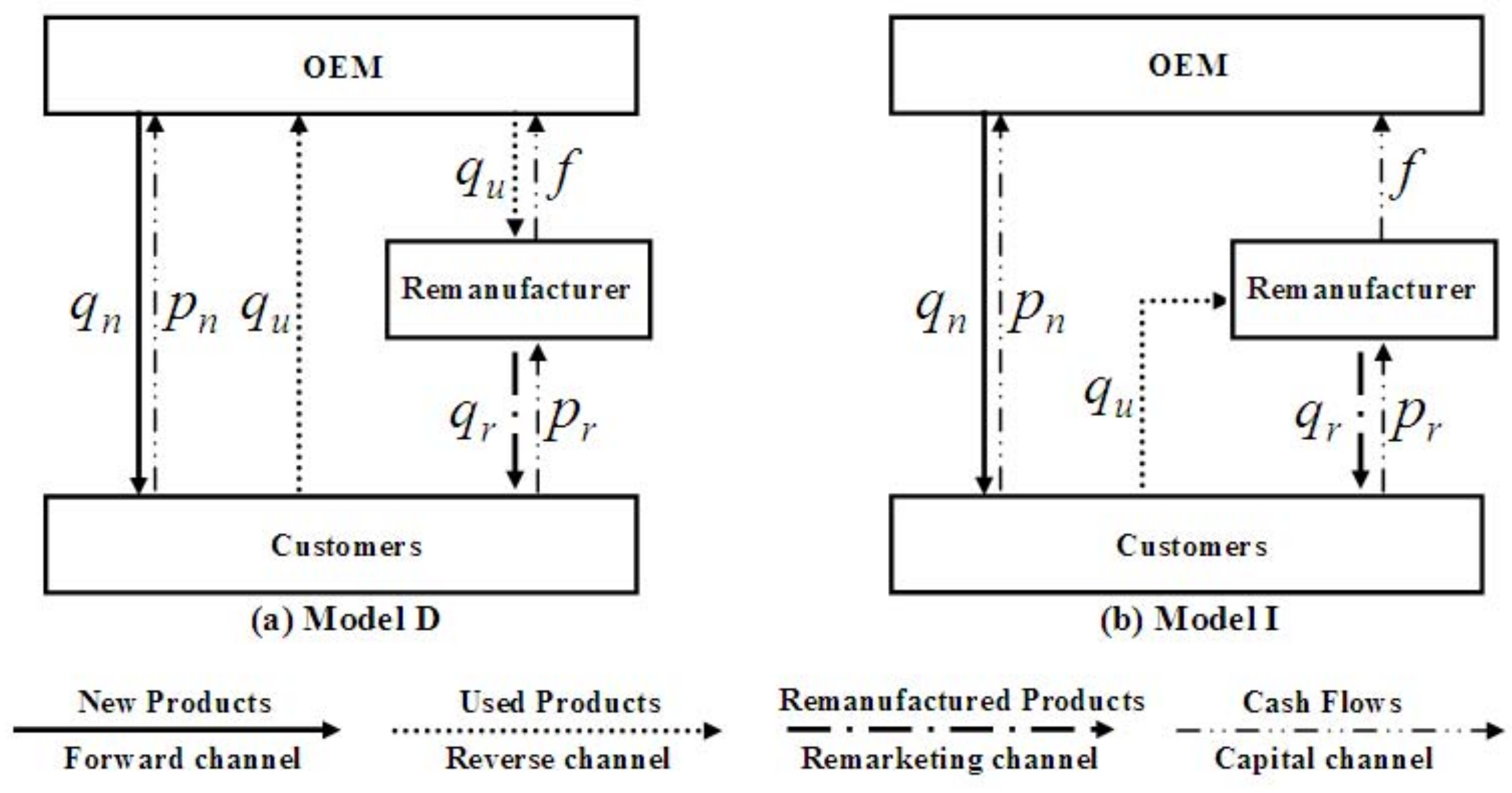
We developed two models of the OEM outsourcing of remanufacturing operations to a TPR, with two options for take-back operations: (i) Model D (direct collection, Figure 1a), where the OEM collects the used products directly from customers; and (ii) Model I (indirect collection, Figure 1b), where the OEM outsources the reverse channel and collects used products indirectly via the TPR. Similar to Savaskan et al. [19] and Yan et al. [30], we assumed that all decisions are considered in a single-period setting. The timing in both models is as follows. First, the OEM announces its patent license fees (f) charged per remanufactured product. Following this, the OEM and the TPR maximize their profits by choosing optimal units of new and remanufactured products ( and ) simultaneously.
Given this basic framework, we next introduce our notation and lay out our assumptions regarding the product, the OEM, the TPR and the consumers. This introduction builds on assumptions commonly used in the remanufacturing literature.
3.1.1. Product
All remanufacturing cores are derived only from new product sales. Similar to the previous studies of Savaskan et al. [19] and Ferrer and Swaminathan [31], we assume that any given unit has only two lives: one as a new product and one as a remanufactured product.
We modelled the reverse channel’s performance as a function of the quantities of used products, which are obtained as remanufacturing cores, (). This is influenced by the product collection effort I (the investment in finding effective demand or providing a certain service level). To characterize the diminishing returns on investment, similar to Savaskan et al. [19], we use the cost structure , where k is a scaling parameter that reflects the collection efficiency.
It is important to note that a strategy’s environmental impact depends on the product volume in each phase multiplied by its per-unit impact in each phase [32,33]. Accordingly, in our analysis, we used and to represent the per-unit disposal impact of the new and remanufactured products. Since remanufacturing requires less material and energy compared to the manufacturing of new products, we further assumed that the per-unit environmental impact of a new product is larger than that of a remanufactured one (essentially, ).
3.1.2. The OEM
We used the usual assumption that the OEM is a Stackelberg leader [30]. The OEM’s problem involves choosing the patent license fee (f) and the units of new products () to maximize its profit () (where refers to the profits for player i under supply chain model j, superscript denotes Model D and Model I, respectively, while subscript denotes the OEM, the TPR, and the total supply chain, respectively). We assumed that the marginal cost to produce a new product is .
3.1.3. The TPR
The TPR is a profit maximizer who offers the remanufactured product to consumers. We assumed that the marginal cost to produce a remanufactured product is . To ensure that making a remanufactured product is less costly than producing a new one, we further assume that according to the finding of Yan et al. [30].
3.1.4. Consumers
One consumer owns at most one product, whether new or remanufactured. The size of the consumer population is assumed to be constant over time and is normalized to 1 [33,34]. Consumers typically differ in their willingness to pay. For this reason, we associate each consumer with their willingness to pay for a new product (u, also called “type”), which is uniformly distributed in the interval of [0, 1]. Consistent with the findings of previous studies [30,35], the primary consumer will discount the value of the remanufactured product to be a fraction of the willingness-to-pay for a new product (i.e., ). Consequently, the demands for the new and remanufactured products are given, respectively, by Equation (1):
The detailed derivations of Equation (1) are provided at the Appendix A.1. All related notations are presented in Table 1.
3.2. Model Formulation and Solution
3.2.1. Model D
In Model D, because the OEM owns the take-back operations and sells them to the TPR, the OEM’s problems are:
where the first term is the revenue obtained from new products, the second term is the revenue derived from remanufactured products, and the last term is the cost of undertaking the product collection.
Given the patent license fee () and anticipating the OEM’s response , the TPR’s problem is:
We solve these problems by using backward induction to determine the subgame perfect equilibrium: once the TPR can maximize its profit by choosing , the OEM can also do so by choosing the quantity of new products (), after which the OEM can choose the patent license fee (). Thus, we can obtain the equilibrium decisions and profits, which is summarized in Table 2 (for clarity, all proofs are provided in the Appendix A.2).
3.2.2. Model I
In Model I, both the take-back and remanufacturing operations are outsourced to the TPR. As a result, the OEM’s problems are:
Given the patent license fee () and anticipating the OEM’s response (), the TPR’s problem is subsequently:
where the first term represents the TPR’s revenue from remanufactured products, while the last term is the core collection cost.
Using backward induction again, we can summarize the equilibrium decisions in Table 2.
4. Model Analysis
Our analysis in this section aims to understand the differences between the two models. To do so, we need to address the questions posed at the beginning of this paper. We started by analyzing the differences in the optimal decisions provided by the models. Subsequently, we enriched our analysis by investigating the differences in the economic, social, and environmental sustainability outcomes of both models.
4.1. Comparison of Optimal Outcomes
Regarding the differences in the patent license fees charged by the OEM under Model D and Model I, we offer the following proposition based on the outcomes presented in Table 2.
Proposition 1.
The OEM is more likely to charge a higher patent license fee in Model D than in Model I (i.e., ).
Not surprisingly, the outsourcing of take-back operations increases the patent license fee charged by the OEM. We mentioned earlier that in Model D, the OEM participates in take-back operations by collecting end-of-life products from consumers and bearing the cost of collection. However, in Model I, such collection costs are paid by the TPR. Hence, as Proposition 1 shows, the OEM usually sets a lower patent license fee to compensate the TPR for their collection costs in Model I .
Comparing the optimal quantities under Model D and Model I establishes the following proposition.
Proposition 2.
(i) Compared to Model I, the OEM provides lesser quantities of new products in Model D, with essentially .
(ii) Compared to Model I, the remanufacturer remanufactures more units in Model D, with essentially .
Proposition 1 shows that, compared to Model D, the OEM is more likely to charge a lower patent license fee in Model I. However, Proposition 2 further reveals that although bearing a lower patent license fee in Model I, the TPR prefers to provide fewer units of remanufactured products. It is important to note that the quantities of remanufactured products vary with changes in two of the model components: this quantity increases when the patent license fee is lowered, but decreases when the OEM increases the number of units sold in the new product market. Thus, Proposition 2 can be interpreted as follows. When the OEM outsources operations to the remanufacturer, the latter component above is always dominant. As a result, although bearing a lower patent license fee in Model I, the TPR prefers to provide fewer units of remanufactured products, as shown in Proposition 2.
4.2. Comparison of Economic Sustainability
Taticchi et al. [36] stated that maximizing supply chain performance and meeting the economic needs of all parties are the two key components of economic sustainability in supply chains. Azevedo et al. [37] and Hariga et al. [38] also focused on economic sustainability with the argument that if a strategy is economically sustainable, it should not only maximize profitability but also be well-supported by all parties. As a result, following this line of research, we highlight economic sustainability from two main perspectives in this subsection. Which strategy is more beneficial to the OEM, the retailer and, in particular, the industry? Is this strategy well supported by all parties? We first looked at the difference in the OEM profitability predicted by the two models.
Proposition 3.
It is more profitable for the OEM to undertake take-back operations directly, with essentially .
Proposition 3 shows that the OEM would benefit more by undertaking take-back operations itself. In order to understand the rationale behind this proposition, it should be noted that in Model D, when the OEM controls the reverse channel, it relies less on adjusting the patent fees charged to the TPR, and sets them more aggressively for profit extraction (see Proposition 1). Therefore, compared to Model I, although the numbers of new products decrease, the numbers of remanufactured products increase (see Proposition 2). As a result, Proposition 3 further reveals that the benefits obtained from remanufactured products under Model D are sufficiently large to compensate for the losses in new product sales.
This observation differs from those of Yu et al. [3], which we believe stems from our model’s focus on whether or not the OEM outsources its take-back operations, rather than whether it centralizes or decentralizes its manufacturing and remanufacturing divisions. This proposition is also inconsistent with the results of Arya et al. [39], who focused on new product marketing in a dual-channel supply chain and argued that an OEM can benefit from decentralized control and the use of transfer prices that are above marginal cost.
After this, we turned our attention to addressing the differences in TPR profitability predicted by the models. We summarize our finding as follows.
Proposition 4.
There exists a threshold such that if , the TPR’s profits in Model D are higher than those in Model I (i.e., ). Otherwise, these profits are lower (i.e., ).
It is important to note that the remanufacturing operations are always undertaken by the TPR in our two models. As a result, the cost of remanufacturing (i.e., ) has no strategic impact on the difference in TPR profitability. However, Proposition 4 shows that, unlike the cost of remanufacturing (i.e., ), the scaling parameter of collection cost plays an important role in determining in both models. In particular, when , the TPR’s profits in Model D are higher than in Model I. It is important to note that the OEM cares greatly about the TPR’s revenue in Model D, because it can derive more profit in Model D than in Model I (see Proposition 3). In particular, when , it means that the collection cost is relatively low and remanufacturing becomes more profitable than producing new products. In order to earn greater profits from remanufacturing, the OEM would produce fewer new products (see Proposition 2). Thus, when , the TPR’s substantial profits stem from the OEM’s desire to obtain greater profitability for the remanufacturer by limiting the output of new products.
We were then able to highlight the differences in industry profit predicted by the models. Based on the outcomes in Table 2, we provided the following proposition.
Proposition 5.
The outsourcing of take-back operations is always detrimental to the industry; that is, .
Propositions 3 and 4 show that the outsourcing of the reverse channel is always beneficial for the OEM but may be detrimental to the TPR (i.e., when , in Proposition 4). Proposition 5 further indicates that the benefits for OEM profitability (see Proposition 3) can “compensate” for TPR’s loss of profit (see Proposition 4). This observation is partially similar to that of Savaskan et al. [19], who concluded that “the total profits in the closed-loop supply channel with OEM collection always dominate the total profits in that with the third-party collection” (p. 246). However, we noted that they did not pay any attention to outsourcing strategies.
Regarding the differences in the economic sustainability of the two models (i.e., the effects of reverse-channel outsourcing on all parties’ profitability) based on Propositions 3–5, we offer the following remark (without proof).
Remark 1.
Compared to outsourcing take-back operations, if , all cores collected by the OEM can create benefits for the OEM, the TPR, and the industry.
The implication of Remark 1 and this subsection is that the ranking of different reverse channel structures (in terms of benefits to the OEM, the TPR, and the industry) indicates which strategy is well supported by all parties. Remark 1 shows that when , OEM-led take-back operations should be supported by all parties.
4.3. Comparison of Environmental Sustainability
In this subsection, we focus on issues of environmental sustainability. Specifically, we intend to answer the question posed at the beginning of this paper: from an environmental sustainability perspective, should manufacturers own or outsource take-back operations, and which is better for the environment? The environmental impact consists of two components, which are namely the impact of new products and the impact of remanufactured products, and can be calculated as follows:
Proposition 6 states that the outsourcing of the reverse channel to a TPR is always detrimental to the environment.
Proposition 6.
Model D is always greener than Model I, with essentially .
Comparing the equilibrium quantities when the OEM performs the take-back operations with those when the TPR fulfils this role, we found that compared to the TPR collection, the OEM (TPR) will provide fewer (more) new (remanufactured) products in Model D according to Proposition 2, with essentially (). As shown by Proposition 6, the total environmental impact predicted by Model D is smaller than that of Model I, due to greater quantities of remanufactured products and fewer new products (i.e., ).
4.4. Comparison of Social Welfare
In this subsection, we studied the differences in social welfare outcomes () between the models. We focused on the social welfare implications of OEMs outsourcing their take-back operations to a TPR. To evaluate the social impact of outsourcing a reverse channel, we compared the optimal welfare values obtained by the two models, where our welfare function includes the consumer willingness-to-pay for remanufactured and new products as well industry profits. Based on the findings of Orsdemir et al. [40] and Yenipazarli [41], our social welfare function consists of three components:
- Consumer surplus, , which consists of two components: consumer willingness-to-pay for remanufactured and new products. It is calculated as follows:
- Industry profits, which follows our definition in Proposition 5.
- Environmental damage, which follows our definition of the disposal impact in Proposition 6.
Comparing the consumer surplus and social welfare outcomes () of the two models, we obtained the following proposition.
Proposition 7.
(i) When , the consumer surplus in Model D is larger than that in Model I (i.e., ). Otherwise, the opposite is true.
(ii) When , the social welfare in Model D is larger than that in Model I (i.e., ). Otherwise, the opposite is true.
Proposition 7 presents an interesting result: if the remanufacturing cost is not pronounced (), there is a larger consumer surplus in Model D than in Model I. In turn, this induces the social welfare of Model D to be higher than that in Model I. It is important to note that the OEM cares greatly about the TPR’s revenue in Model D, because it can derive greater profit in Model D than in Model I (see Proposition 3). In particular, when , the OEM would let the third party remanufacture more cores in order to earn more profits from remanufactured products (, in Proposition 2). On the other hand, in order to provide more cores for remanufacturing, the level of availability of new products in Model D is larger than that in Model I, with essentially . Said differently, when cr < c1, the competition between new products and remanufactured ones in Model D becomes stronger than that in Model I, which benefits consumers (CSD* > CSI*). When remanufacturing costs are pronounced (i.e., cr > c1, the opposite is true. Proposition 7 further shows that when remanufacturing costs are pronounced (i.e., ), the benefits to industry profitability predicted by Model D (see Proposition 5) are insufficient in fully compensating for the loss in consumer surplus compared to Model I, though the environmental damage of Model D is lower than that of Model I (see Proposition 6). Hence, when , the social welfare predicted by Model D is smaller than that in Model I.
In the analysis thus far, we have considered cases where the OEM undertakes take-back operations directly or indirectly, with several interesting results found from economic, social, and environmental perspectives. In order to have a more comprehensive understanding of when to outsource remanufacturing, whether manufacturers should own or outsource their take-back operations, we present the following remark (without proof), which is based on Remark 1 and Propositions 6 and 7.
Remark 2.
Compared to outsourcing take-back operations, if and , then manufacturers undertaking take-back operations can create an overall beneficial outcome that meets the economic, environmental, and social sustainability.
Remark 2 reveals that, under certain conditions, manufacturers undertaking take-back operations can achieve inherent economic, social, and environmental benefits. Put differently, when remanufacturing operations are undertaken by a TPR, the take-back operations undertaken by the OEM do not necessarily harm the third party. On the contrary, controlling the reverse channel can achieve gains in terms of economic, social, and environmental sustainability.
4.5. Numerical Example
From a managerial perspective, our analysis highlights how the strategies of owning or outsourcing take-back operations have strategic consequences in terms of economic, environmental, and social issues. To better emerge in how the parameters—in particular, the remanufacturing cost—affect the performance of sustainability under two different models, in this section we reanalyze the economic, environmental, and social outcomes using numerical examples.
In our numerical examples, in order to examine the impacts of the remanufacturing cost () on the economic, environmental, and social outcomes, the parameters about the production cost and the scaling parameter of collection cost are characterized by and , respectively. We set the consumer value discount for the remanufactured product () to 0.9 (i.e., ). The per-unit disposal impact of the new/remanufactured product is and , respectively. Ensuring that all parameters and variables in this paper must satisfy non-negativity constraints, we let ; that is, in our numerical examples, . All figures are obtained from numerical simulation in Matlab 2014.
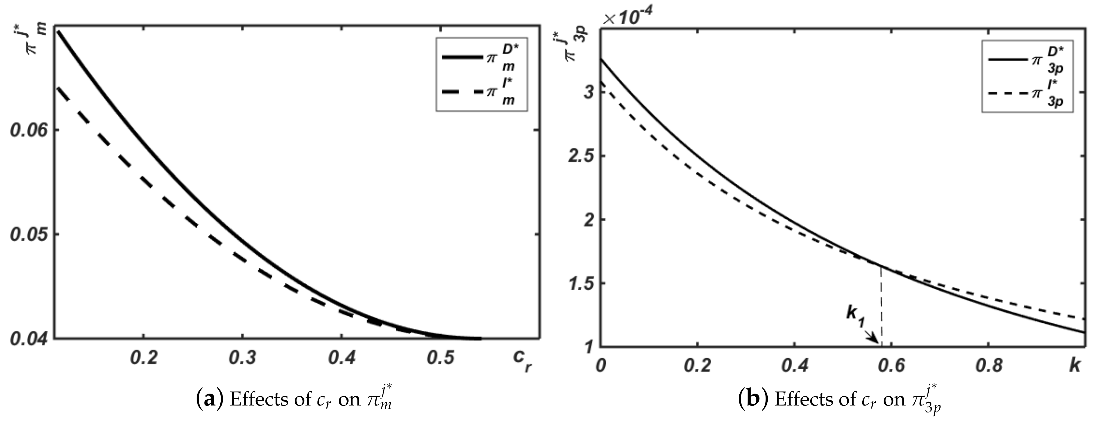
We first present three figures of results for economic outcomes. Figure 2 reports the profits of the OEM, TPR, and industry on both models. As illustrated in Figure 2a, we can obtain that the manufacturer’s profit in Model D is always larger than that in Model I (i.e., ). In addition, the difference in the manufacturer’s profitability between both models decreases with . Similarly, as Figure 2c shows, the industry profits in Model D are always higher than that in Model I, and furthermore, as the remanufacturing cost, , increases, the difference between both profits decreases. The variations in the TPR’s profits in both models are as shown in Figure 2b. Based on Figure 2b, we find that there exists a threshold ; when , the third-party remanufacturer’s profits in Model D are higher than those in Model I (i.e., ); but are lower (i.e., ) otherwise. In sum, based on Figure 2, we can conclude our results in Remark 1.
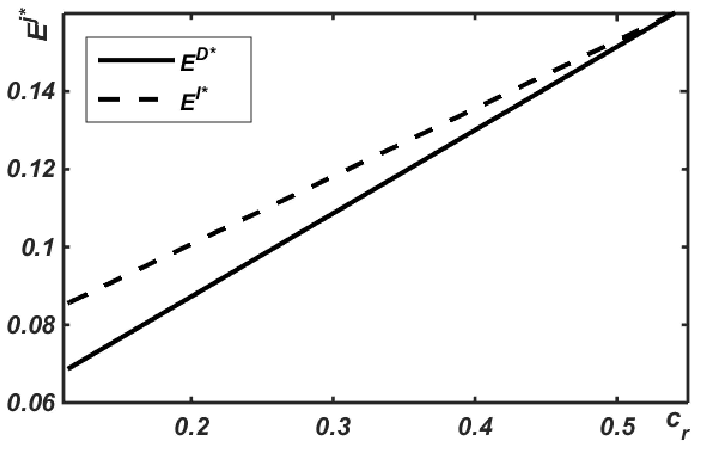
We are now in a position to address the effects of the remanufacturing cost on the environmental outcomes, (see Figure 3). Figure 3 illustrates two important phenomena: First, the environmental impact in Model D is always smaller than that in Model I. Second, as increases, the difference in environmental impacts between the two models decreases.
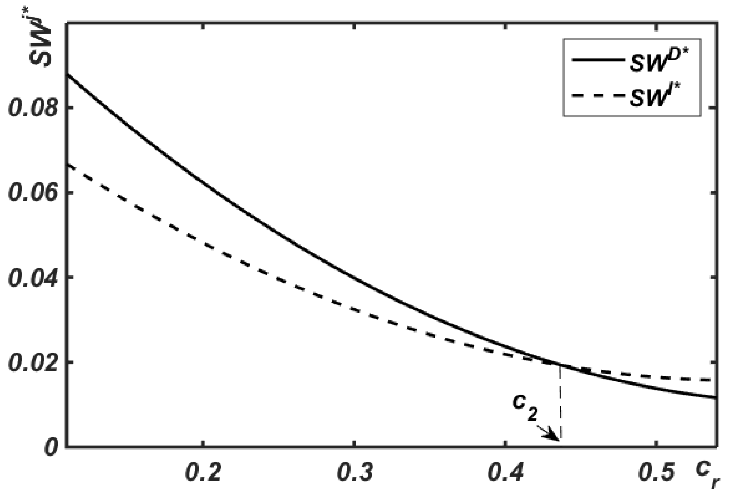
Finally, we analyze the difference in social welfare between the two models. Based on Figure 4, we find that both and decrease with the remanufacturing cost of . Furthermore, there exists a threshold ; when , the social welfare in Model D is larger than that in Model I (i.e., ); otherwise, the opposite is true.
5. Conclusions
Despite the fact that remanufacturing has been demonstrated to have economic, social, and environmental benefits, few OEMs engage in remanufacturing themselves as they instead outsource it to a TPR. It is important to note that the outsourcing of remanufacturing is not a purely make-or-buy decision, but involves a reverse channel that determines the rate of core return from customers and affects the performance of forward channel decisions. In practice, there are two different options or modes that OEMs can use when considering take-back operations. Many OEMs that outsource their remanufacturing activities still control the reverse channel by collecting end-of-life products from consumers, which protects the sales of new products. Meanwhile, other OEMs outsource collection activities to TPRs. This raises the question of whether OEMs should also outsource their reverse channels to TPR, especially considering the issues that the outsourcing of remanufacturing raises between the OEMs and the TPR. To answer this strategic question, we need to understand the optimal strategy for each party.
We developed two models to better understand the effects of outsourcing the reverse channel to a TPR or keeping it in-house. We examined the implications of each strategy for economic, environmental, and social sustainability. Therefore, our paper makes the following contributions to the remanufacturing literature. First, rather than focusing on outsourcing issues between OEMs and TPRs, we provide an alternative and partially complementary approach that considers the outsourcing of take-back operations. Second, although reverse supply chains for recycling have been thoroughly studied in terms of logistics network design, operational planning, and channel operation organization, little is known about how owning or outsourcing take-back operations affects sustainability issues. In particular, our finding of the economic, social, and environmental benefits of take-back operations managed by OEMs has implications for both academics and managers.
We do acknowledge a few limitations of our models. First, we assumed a monopoly OEM, complete information, and no consumer preference—all of which could be relaxed in future research. Second, to keep our focus on our research questions, we assumed that all decisions were considered in a single-period setting. While this assumption is common in the remanufacturing literature [19,30,40], it does not reflect the relationship between a product’s lifecycle and remanufacturing decisions. Third, we viewed OEMs as producers of new products and did not allow them to engage in remanufacturing. However, there are also situations where remanufacturing is unappealing to third parties yet attractive to OEMs. The competitive relationship between an OEM and their TPRs could be an interesting research question for future work. Finally, in both of our models, the quantities of remanufactured products were limited by the availability of new products. Without this limitation, the results obtained may be different.
Acknowledgments
The authors thank National Natural Science Foundation of China (71531003, 71472026, 71672020, 71272127, 71272130 and 71572030), the Humanities and Social Sciences Foundation for Young Scholars of China’s Ministry of Education (15YJC630154), and the Fundamental Research Funds for the Central Universities (ZYGX2015KYQD080) for supporting this research.
Author Contributions
Wei Yan contributed to model development; Hengyu Li contributed to writing; Junwu Chai contributed to strengthen all results’ interpretaion; Zhifeng Qian provided revised advice. Hong Chen provided motivation cases. All authors read and approved the final manuscript.
Conflicts of Interest
The authors declare no conflict of interest.
Appendix A. Proofs of Statements
- To accommodate space constraints, we will only provide a sketch of the proofs for some results. A detailed analysis of these results is available from the authors upon request.
- All parameters and variables in this paper must satisfy non-negativity constraints; that is, we only consider .
Appendix A.1. Technical Analysis for Both Models
Appendix A.1.1. Proof of Inverse Demand Functions
In our models, a consumer has three different options: not buying any products, buying a new product, or buying a remanufactured product. Accordingly, as shown in Figure A1, those who are willing to pay for the new good from OEM derive a net utility of ; those with next lower u values belong to the remanufactured products (); those with the lowest u values do not buy any product and derive a net utility of . The class division points are found by setting the net present value functions in adjacent regions equal to each other. That is, the indifferent point between buying a new product or a remanufactured product from the OEM is at . Similarly, the indifferent point between buying a remanufactured product and not buying is at .
Specifically, . Much empirical evidence has proved the consumer willingness-to-pay for the remanufactured products is lower than that for the new products, which represents a vertical differentiation between the two products. Therefore, the total sales quantity from the new product is and the total number of units acquired from the remanufactured product is given by . This gives rise to the inverse demand functions in Equation (1).
Figure A1.
Net present value functions for consumer.

Appendix A.1.2. Proof of Model D
Plugging Equation (1) into the OEM’s and third party’s profit, we can obtain that and . Solving the first-order condition of these formulas with respect to and , respectively, yields:
Plugging and into the OEM’s profits and yields, that is,
The first-order condition of this formula with respect to f yields . Then, we easily show the optimal .
Substituting into the , , OEM’s profits, consumer surplus and environmental impacts get the rest equilibrium outcomes in Model D. We notice that all parameters and variables must satisfy nonnegativity constraints. Then, we solve the parameter scope of these nonlinear conditions: , iff .
Appendix A.1.3. Proof of Model I
Plugging Equation (1) into the OEM’s and third party’s profit, we can obtain that and . Solving the first-order condition of these formulas with respect to and , respectively, yields :
Plugging and into the OEM’s profits and yields
The first-order condition of this formula with respect to f yields . Then, we easily show the optimal .
Substituting into the , , OEM’s profits, consumer surplus and environmental impacts get the rest equilibrium outcomes in Model D. We notice that all parameters and variables must satisfy nonnegativity constraints. Then, we solve the parameter scope of these nonlinear conditions: , iff . Then, we compare the range of the threshold and the threshold , and make sure the comparative range is under the threshold . In the range of the threshold , we compare the outcomes between Model D and Model I and draw the Proposition 1, 2, 3, 4, 5, 6, and 7.
Appendix A.2. Proofs
Appendix A.2.1. Proof of Proposition 1
To prove , we have to show that , that is, , after simplification, for any k and in the range of the threshold , we can obtain that , and always hold. Therefore, always hold.
Appendix A.2.2. Proof of Proposition 2
- (i)
- To prove , we have to show that , that is, , after simplification, for any k and in the range of the threshold , we can obtain that and always hold. Therefore, always hold.
- (ii)
- To prove , we have to show that , that is, , after simplification, for any k and in the range of the threshold , we can obtain that and always hold. Therefore, always hold.
Appendix A.2.3. Proof of Proposition 3
To prove , we have to show that , that is, , after simplification, for any k and in the range of the threshold , we can obtain that and always hold. Therefore, always hold.
Appendix A.2.4. Proof of Proposition 4
Comparing the third party’s profit for the product between Model D and Model I. We obtain a threshold , iff , ; to prove that, we have to show that , that is, after simplification, for any k and in the range of the threshold , we can obtain that and always hold. Therefore, always hold. On the contrary, when , always hold.
Appendix A.2.5. Proof of Proposition 5
Comparing the whole channel’s profit between Model D and Model I. We give , to prove , we have to show that ; that is, , after simplification, for any k and in the range of the threshold , we can obtain that and always hold. Therefore, always hold.
Appendix A.2.6. Proof of Proposition 6
Since remanufacturing can eliminate the returned cores’ disposal impact, the total disposal impact of new products is ; meanwhile, the total disposal impact of remanufactured products is . Thus, the total disposal impact in Model D and Model I are and , respectively. We can easily show that , because , , and . Thus, , meaning that the Model D is greener than Model I.
Appendix A.2.7. Proof of Proposition 7
- (i)
- Comparing the consumer surplus between Model D and Model I. We obtain a threshold , iff , , to prove that, we have to show that ; that is, , after simplification, we get a threshold , when , both numerator and denominator are positive, always hold. On the contrary, when , always hold.
- (ii)
- Comparing the social welfare between Model D and Model I. We obtain a threshold , iff , , to prove that, we have to show that ; that is, , after simplification, we get a threshold , when , both numerator and denominator are positive, always hold. On the contrary, when , always hold.
References
- Dyllick, T.; Kai, H. Beyond the business case for corporate sustainability. Bus. Strategy Environ. 2002, 11, 130–141. [Google Scholar] [CrossRef]
- White, L.; Lee, G.J. Operational research and sustainable development: Tackling the social dimension. Eur. J. Oper. Res. 2009, 193, 683–692. [Google Scholar] [CrossRef]
- Zhou, Y.; Xiong, Y.; Li, G.; Xiong, Z.; Beck, M. The bright side of manufacturing-remanufacturing conflict in a decentralised closed-loop supply chain. Int. J. Prod. Res. 2013, 51, 2639–2651. [Google Scholar] [CrossRef]
- Ferguson, M. Strategic Issues in Closed-Loop Supply Chains with Remanufacturing. Available online: http://citeseerx.ist.psu.edu/viewdoc/download?doi=10.1.1.151.6643&rep=rep1&type=pdf (accessed on 8 January 2018).
- Ferguson, M.E.; Souza, G.C. Closed-Loop Supply Chains: New Developments to Improve the Sustainability of Business Practices; Ferguson, M.E., Souza, G.C., Eds.; CRC Press: Boca Raton, FL, USA, 2010; p. 257. [Google Scholar]
- Pagell, M.; Wu, Z.; Murthy, N.N. The supply chain implications of recycling. Bus. Horiz. 2007, 50, 133–143. [Google Scholar] [CrossRef]
- Gutowski, T.G.; Murphy, C.F.; Allen, D.T.; Bauer, D.J.; Bras, B.; Piwonka, T.S.; Sheng, P.S.; Sutherland, J.W.; Thurston, D.L.; Wolff, E.E. Environmentally Benign Manufacturing; World Technology (WTEC) Division, International Technology Research Institute: Baltimore, MD, USA, 2001. [Google Scholar]
- The Auto Channel, Caterpillar Remanufacturing Services Forms Strategic Alliance With Land Rover. Available online: https://www.theautochannel.com/news/2005/08/04/139416.html2017 (accessed on 14 November 2017).
- Hauser, W.M.; Lund, R.T. The Remanufacturing Industry: Anatomy of a Giant: A View of Remanufacturing in America Based on a Comprehensive Survey across the Industry. Department of Manufacturing Engineering. Available online: www.bu.edu/reman2008 (accessed on 18 October 2017).
- Fleischmann, M.; Bloemhof-Ruwaard, J.M.; Dekker, R.; Van der Laan, E.; Van Nunen, J.A.; Van Wassenhove, L.N. Quantitative models for reverse logistics: A review. Eur. J. Oper. Res. 1997, 103, 1–17. [Google Scholar] [CrossRef] [Green Version]
- Marion, J. Sun Under Fire—For Fixing Solaris OS Costs to Reduce Competition in Used Sun Market. Available online: http://www.sparcproductdirectory.com/view56.html2004 (accessed on 18 November 2017).
- Karakayali, I.; Emir-Farinas, H.; Akcali, E. An analysis of decentralized collection and processing of end-of-life products. J. Oper. Manag. 2007, 25, 1161–1183. [Google Scholar] [CrossRef]
- Rahman, S.; Subramanian, N. Subramanian, Factors for implementing end-of-life computer recycling operations in reverse supply chains. Int. J. Prod. Econ. 2012, 140, 239–248. [Google Scholar] [CrossRef]
- Zou, Z.-B.; Wang, J.J.; Deng, G.-S.; Chen, H. Third-party remanufacturing mode selection: Outsourcing or authorization? Transp. Res. Part E Logist. Transp. Rev. 2016, 87 (Suppl. C), 1–19. [Google Scholar] [CrossRef]
- Majumder, P.; Groenevelt, H. Competition in remanufacturing. Prod. Oper. Manag. 2010, 10, 125–141. [Google Scholar] [CrossRef]
- Jin, M.; Nie, J.; Yang, F.; Zhou, Y. The impact of third-party remanufacturing on the forward supply chain: A blessing or a curse? Int. J. Prod. Res. 2017, 55, 6871–6882. [Google Scholar] [CrossRef]
- Huang, M.; Yi, P.; Shi, T. Triple Recycling Channel Strategies for Remanufacturing of Construction Machinery in a Retailer-Dominated Closed-Loop Supply Chain. Sustainability 2017, 9, 2167. [Google Scholar] [CrossRef]
- Govindan, K.; Soleimani, H.; Kannan, D. Reverse logistics and closed-loop supply chain: A comprehensive review to explore the future. Eur. J. Oper. Res. 2015, 240, 603–626. [Google Scholar] [CrossRef] [Green Version]
- Savaskan, R.C.; Bhattacharya, S.; Wassenhove, L.N.V. Closed-Loop Supply Chain Models with Product Remanufacturing. Manag. Sci. 2004, 50, 239–252. [Google Scholar] [CrossRef]
- Ordoobadi, S.M. Outsourcing reverse logistics and remanufacturing functions: A conceptual strategic model. Manag. Res. News 2009, 32, 831–845. [Google Scholar] [CrossRef]
- Hong, X.; Wang, Z.; Wang, D.; Zhang, H. Decision models of closed-loop supply chain with remanufacturing under hybrid dual-channel collection. Int. J. Adv. Manuf. Technol. 2013, 68, 1851–1865. [Google Scholar] [CrossRef]
- Alshamsi, A.; Diabat, A. A reverse logistics network design. J. Manuf. Syst. 2015, 37 Pt 3, 589–598. [Google Scholar] [CrossRef]
- Eskandarpour, M.; MasehianEmail, E.; Soltani, R.; Khosrojerdi, A. A reverse logistics network for recovery systems and a robust metaheuristic solution approach. Int. J. Adv. Manuf. Technol. 2014, 74, 1393–1406. [Google Scholar] [CrossRef]
- Daaboul, J.; Le Duigou, J.; Penciuc, D.; Eynard, B. Reverse logistics network design: A holistic life cycle approach. J. Remanuf. 2014, 4, 1–7. [Google Scholar] [CrossRef]
- Shulman, J.D.; Coughlan, A.T.; Savaskan, R.C. Optimal Reverse Channel Structure for Consumer Product Returns. Mark. Sci. 2010, 29, 1071–1085. [Google Scholar] [CrossRef]
- Hsieh, C.C.; Chang, Y.L.; Wu, C.H. Competitive pricing and ordering decisions in a multiple-channel supply chain. Int. J. Prod. Econ. 2014, 154, 156–165. [Google Scholar] [CrossRef]
- Gumus, M.; Ray, S.; Yin, S. Returns Policies Between Channel Partners for Durable Products With Used Goods Markets. Mark. Sci. 2013, 32, 622–643. [Google Scholar] [CrossRef]
- Neto, J.Q.F.; Walther, G.; Bloemhof, J.; Van Nunen, J.A.; Spengler, T. A methodology for assessing eco-efficiency in logistics networks. Eur. J. Oper. Res. 2009, 193, 670–682. [Google Scholar] [CrossRef]
- Liu, H.; Yue, X.; Ding, H.; Leong, G.K. Optimal Remanufacturing Certification Contracts in the Electrical and Electronic Industry. Sustainability 2017, 9, 516. [Google Scholar] [CrossRef]
- Yan, W.; Xiong, Y.; Xiong, Z.; Guo, N. Bricks vs. clicks: Which is better for marketing remanufactured products? Eur. J. Oper. Res. 2015, 242, 434–444. [Google Scholar] [CrossRef]
- Ferrer, G.; Swaminathan, J.M. Managing new and differentiated remanufactured products. Eur. J. Oper. Res. 2010, 203, 370–379. [Google Scholar] [CrossRef] [Green Version]
- White, A.L.; Stoughton, M.; Feng, L. Servicizing: The Quiet Transformation to Extended Producer Responsibility. Available online: http://infohouse.p2ric.org/ref/17/16433.pdf (accessed on 8 January 2018).
- Agrawal, V.V.; Thomas, V.M. Is Leasing Greener than Selling? Manag. Sci. 2012, 58, 523–533. [Google Scholar] [CrossRef]
- Ferguson, M.E.; Toktay, L.B. The Effect of Competition on Recovery Strategies. Prod. Oper. Manag. 2006, 15, 351–368. [Google Scholar] [CrossRef]
- Debo, L.G.; Toktay, L.B.; Wassenhove, L.N.V. Market Segmentation and Product Technology Selection for Remanufacturable Products. Manag. Sci. 2005, 51, 1193–1205. [Google Scholar] [CrossRef]
- Taticchi, P.; Tonelli, F.; Pasqualino, R. Performance measurement of sustainable supply chains: A literature review and a research agenda. Int. J. Prod. Perform. Manag. 2013, 62, 782–804. [Google Scholar] [CrossRef]
- Azevedo, S.G.; Carvalho, H.; Ferreira, L.M.; Matias, J.C.O. A proposed framework to assess upstream supply chain sustainability. Environ. Dev. Sustain. 2017, 19, 2253–2273. [Google Scholar] [CrossRef]
- Hariga, M.; As’ad, R.; Shamayleh, A. Integrated economic and environmental models for a multi stage cold supply chain under carbon tax regulation. J. Clean. Prod. 2017, 166 (Suppl. C), 1357–1371. [Google Scholar] [CrossRef]
- Arya, A.; Mittendorf, B.; Yoon, D.H. Friction in Related-Party Trade When a Rival Is Also a Customer. Manag. Sci. 2008, 54, 1850–1860. [Google Scholar] [CrossRef]
- Orsdemir, A.; Kemahlioglu-Ziya, E.; Parlakturk, A.K. Competitive Quality Choice and Remanufacturing. Prod. Oper. Manag. 2014, 23, 48–64. [Google Scholar]
- Yenipazarli, A. Managing new and remanufactured products to mitigate environmental damage under emissions regulation. Eur. J. Oper. Res. 2016, 249, 117–130. [Google Scholar] [CrossRef]
Figure 1.
The two basic models. OEM: original equipment manufacturer.

Figure 2.
Effects of on the economic outcomes.


Figure 3.
Effects of on .

Figure 4.
Effects of on .


Table 1.
Parameters and decision variables.
| Notation | Definition |
|---|---|
| k | Scaling parameter of collection cost |
| u | Consumer willingness-to-pay for the new product |
| Consumer value discount for the remanufactured product | |
| f | Patent license fee per remanufactured product |
| Profits for player i under supply chain model j | |
| // | Production quantity of the new/remanufactured/used product |
| / | The price for the new/remanufactured product |
| / | Unit production cost of the new/remanufactured product |
| / | Per-unit disposal impact of the new/remanufactured product |
Table 2.
Equilibrium decisions and profits.
| The OEM Collects Cores (Direct Collection, Model D) |
| The TPR Collects Cores (Indirect Collection, Model I) |
© 2018 by the authors. Licensee MDPI, Basel, Switzerland. This article is an open access article distributed under the terms and conditions of the Creative Commons Attribution (CC BY) license (http://creativecommons.org/licenses/by/4.0/).
Share and Cite
MDPI and ACS Style
Yan, W.; Li, H.; Chai, J.; Qian, Z.; Chen, H. Owning or Outsourcing? Strategic Choice on Take-Back Operations for Third-Party Remanufacturing. Sustainability 2018, 10, 151. https://doi.org/10.3390/su10010151
AMA Style
Yan W, Li H, Chai J, Qian Z, Chen H. Owning or Outsourcing? Strategic Choice on Take-Back Operations for Third-Party Remanufacturing. Sustainability. 2018; 10(1):151. https://doi.org/10.3390/su10010151
Chicago/Turabian StyleYan, Wei, Hengyu Li, Junwu Chai, Zhifeng Qian, and Hong Chen. 2018. "Owning or Outsourcing? Strategic Choice on Take-Back Operations for Third-Party Remanufacturing" Sustainability 10, no. 1: 151. https://doi.org/10.3390/su10010151
Note that from the first issue of 2016, this journal uses article numbers instead of page numbers. See further details here.