Monitoring of ULF (Ultra-Low-Frequency) Geomagnetic Variations Associated with Earthquakes


1
Department of Electronic Engineering and Research Station on Seismo Electromagnetics, The University of Electro-Communications, 1-5-1 Chofugaoka, Chofu, Tokyo 182-8585, Japan
2
Faculty of Science, Chiba University, 1-33 Yayoi, Inage Chiba 263-8522, Japan
3
Department of Electronics, Chubu University, 1200 Matsumoto-cho, Kasugai, Aichi 487-8501, Japan
*
Author to whom correspondence should be addressed.
Sensors 2007, 7(7), 1108-1122; https://doi.org/10.3390/s7071108
Submission received: 14 June 2007
/
Accepted: 26 June 2007
/
Published: 4 July 2007
(This article belongs to the Special Issue Sensors for Disaster and Emergency Management Decision Making)
Abstract
:ULF (ultra-low-frequency) electromagnetic emission is recently recognized as one of the most promising candidates for short-term earthquake prediction. This paper reviews previous convincing evidence on the presence of ULF emissions before a few large earthquakes. Then, we present our network of ULF monitoring in the Tokyo area by describing our ULF magnetic sensors and we finally present a few, latest results on seismogenic electromagnetic emissions for recent large earthquakes with the use of sophisticated signal processings.
1. Introduction
It has been recently reported that electromagnetic phenomena take place in a wide frequency range prior to an earthquake (1) ∼ (3), and these precursory seismo-electromagnetic effects are expected to be useful for the mitigation of earthquake hazards. Basically there are two principal methods of observation of earthquake signatures. The first is the direct observation of electromagnetic emissions (natural emissions) from the lithosphere and the second is to detect indirectly the seismic effect taken place in a form of propagation anomaly of the pre-existing transmitter signals (we call it radio sounding). The first method is based on the idea that natural emissions are radiated from the hypocenter of earthquakes due to some tectonic effect during their preparation phase. The second is based on the idea that there take place the anomalies in the atmosphere and ionosphere due to the seismicity, leading to the generation of propagation anomaly on the pre-existing transmitter signal characteristics (amplitude and phase). This paper deals with the ULF (ultra-low-frequency, with frequency less than 10 Hz) magnetic field variation belonging to the first category. The study on seismogenic ULF emissions started in the early 1990s. Even though the radio emissions are generated as a pulse in the earthquake hypocenter, higher frequency components cannot propagate over long distances in the lithosphere due to severe attenuation, but ULF waves can propagate up to an observation point near the Earth's surface with small attenuation. This is the most important advantage of seismogenic ULF emissions.
There have been reported three reliable events for the ULF magnetic field variations prior to the earthquakes; (1) Armenia, Spitak earthquake (1988 December 8, Magnitude = 6.9) (4), (2) USA, California, Loma Prieta earthquake (1989 October 18, M = 7.1) (5), and (3) Guam earthquake (1993 August 8, M = 8.0) (6). The epicentral distance is 129 km for (1), 7 km for (2) and 65 km for (3) (4)-(6). The Loma Prieta earthquake happened very close to the observing station, so that it is better for us to indicate the results for this earthquake. Fig. 1 illustrates the temporal evolution of ULF magnetic field (horizontal component, frequency = 0.01 Hz (period = 100 s)). It indicates that the magnetic field increases for about one week 5-12 days before the earthquake, followed by a quiet period and a sharp increase one day before the earthquake (especially an abrupt increase 3-4 hours before the earthquake). Very significant changes in ULF magnetic field were also observed for other two earthquakes, which was a stimulus to the extensive research on the relationship of ULF emissions and earthquakes. In this paper we review the relationship between the two. An additional important point is that these seismogenic ULF emissions are so weak that it is of essential importance for us to develop any methods to identify those signals. We need sophisticated methods of signal processing, and we review the observational results by those methods. Finally, we will comment on our future works.
2. Magnetic field sensors and observation system
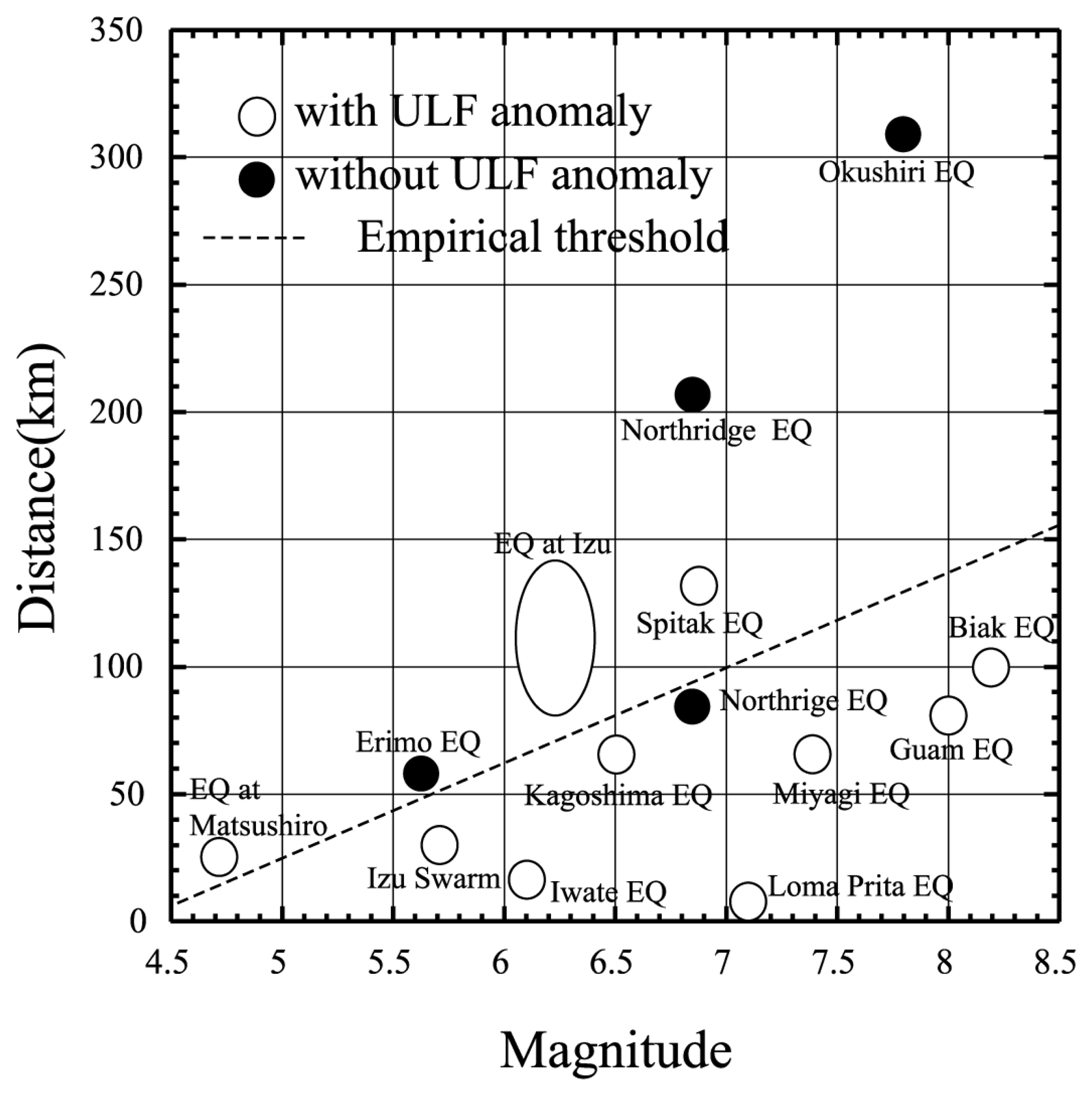
Fig.2 shows the summary on the occurrence of the earthquake-related ULF activity in the form of earthquake magnitude (M) versus epicentral distance (R) from a ULF magnetic station. White and black circles show an earthquake with and without ULF anomalies, respectively. The dashed line indicates the empirical threshold (0.025R≦ M-4.5) for the appearance of anomalous ULF signals preceding large earthquakes. This figure demonstrates that ULF emissions could be observed about 60 km from the source region for an earthquake with M≧ 6, and the detectable distance of ULF magnetic anomalies would be extended to about 100 km in the case of an earthquake with M≧ 7. The details of those earthquakes in Fig.2 are described in Hattori (2006) (7) and Hayakawa et al. (2004) (8).
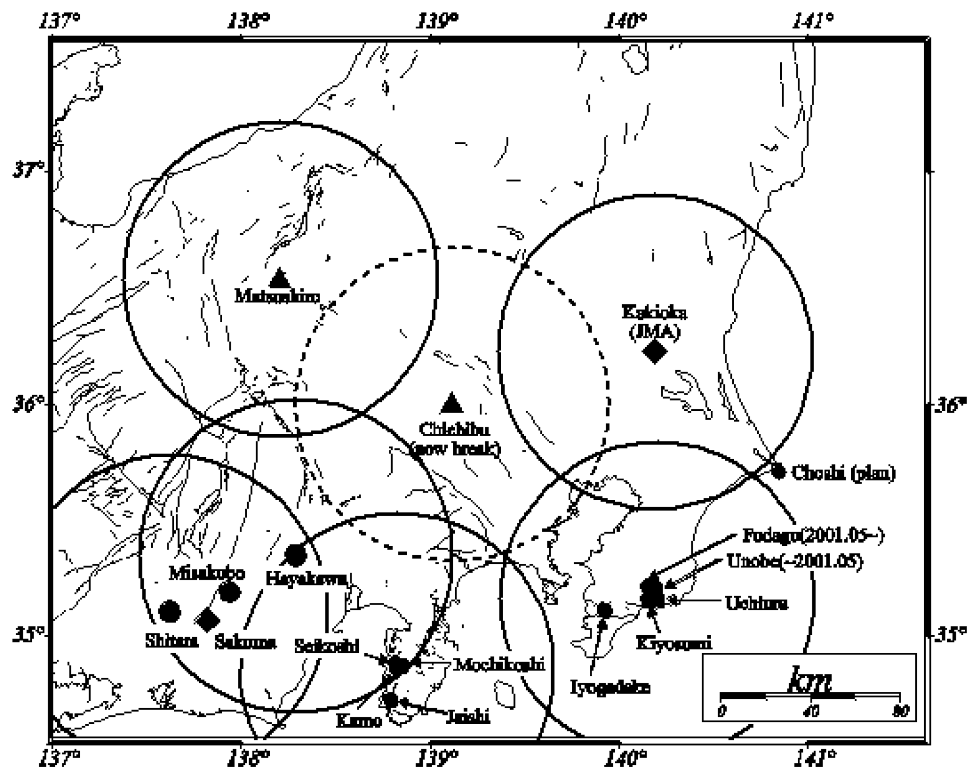
It is important to predict earthquakes with M≧ 6 in a highly populated region to mitigate disasters. Therefore, we decided to install a network of ULF magnetometers with high sampling rate to cover the Kanto (Tokyo) area with inter-sensor distances of about 70-80 km. Two types of magnetometers are adopted; torsion and induction types. Taking account of the existence of Kakioka Geomagnetic Observatory, Japan Meteorological Agency (JMA) (36.2°N, 144.2°E), we planned to set up stations to cover the area, as shown in Fig.3. Circles in the figure indicate the distance of 60 km from the station (the circle from Kakioka observatory is also displayed). The clock system at each station is controlled by GPS. The information on all of our stations is summarized in Table 1.
One of the sensors (induction magnetometer) has been installed, for example, in JMA's Matsushiro Seismological Observatory (36.5°N, 138.2°E), in which strain meters, tilt meters, and short-period seismometers are already in operation by JMA. A comparison between the seismic and electromagnetic data will be useful in understanding the fundamental physics of the earthquake preparation process. We also installed the induction magnetometer at Chichibu station. Induction magnetometers installed at these two stations are search coil type with 85 Hz sampling rate, named LEMI-30 produced by Lviv Center of Institute of Space Research, National Academy of Science of Ukraine. These sensors are intended for the study of frequency band from 0.01 to 30 Hz, and detailed specification of them is summarized in Hattori et al. (2004) (7). Also the acoustic emission sensor was installed at Matsushiro station. The acoustic sensor records the emissions at four frequency bands of 30, 160, 500, and 1000Hz. The lowest band corresponds to the uppermost frequency of LEMI-30.
A small L-shaped array has been composed with three torsion magnetometers, the distance of which is about 5 km at the western part of Izu peninsula and the southern part of Boso peninsula. With these arrays, we expect to develop a method to find the arrival direction of ULF waves (8). Both Izu and Boso Peninsulas are seismic active regions, so that we consider it good for precise observation for direction finding of ULF anomalous signals by means of the arrays. We also installed torsion magnetometers at Jaishi, Iyogatake, Hayakawa, Misakubo, and Shitara. These torsion magnetmeters, MVC-2DS, were produced by Institute of Terrestrial Magnetism, Ionosphere and Radiowave Propagation, Saint Petersburg Filial (SPbF IZMIRAN), Russian Academy of Sciences. A magneto-sensitive element of the torsion sensor is a permanent magnet suspended with quartz or metallic fibers which serve as the rotation axis of the magneto-sensitive element. The reflecting surface which transforms angular displacement of the magneto-sensitive element into electric signal by means of photoelectric converter is mounted rigidly to the magnetic-sensitive element. When the element is turned by the force of the external magnetic field, the light beam deviates from the zero position, leading to an increase of one diode illumination and a decrease of the other. As a result, there appears a signal proportional to the disturbed magnetic field value for the sensor output. The element is suspended inside the fluid-filled capsule on the thin metallic fibers and a low-powered monochromatic infra-red emitting diode is used for the photo emitter. The feedback circuit which produces a magnetic field opposite to the external field are adopted. Also the coil for current compensation of constant magnetic field to set up the magnetic-sensitive element at the zero position and the coil for calibration are installed. The main technical parameters of MVC-2DS are described in Hattori et al. (2004) (7).
Some fluxgate (3 components) magnetometers have been installed in addition to the above-mentioned ULF network, which are JCS-107F (Chiba Electronics Inc.: frequency range ∼1 Hz), which is effective for much lower frequency (nearly DC).
3. Analysis method of ULF magnetic field variations
In addition to the installation of highly sensitive ULF sensors, we have to carry out sophisticated signal processing in order to detect and identify weak seismogenic ULF emissions. We have already developed several useful signal processings, some of which will be described below.
3.1. The ratio of vertical to horizontal components of the magnetic field (polarization analysis)
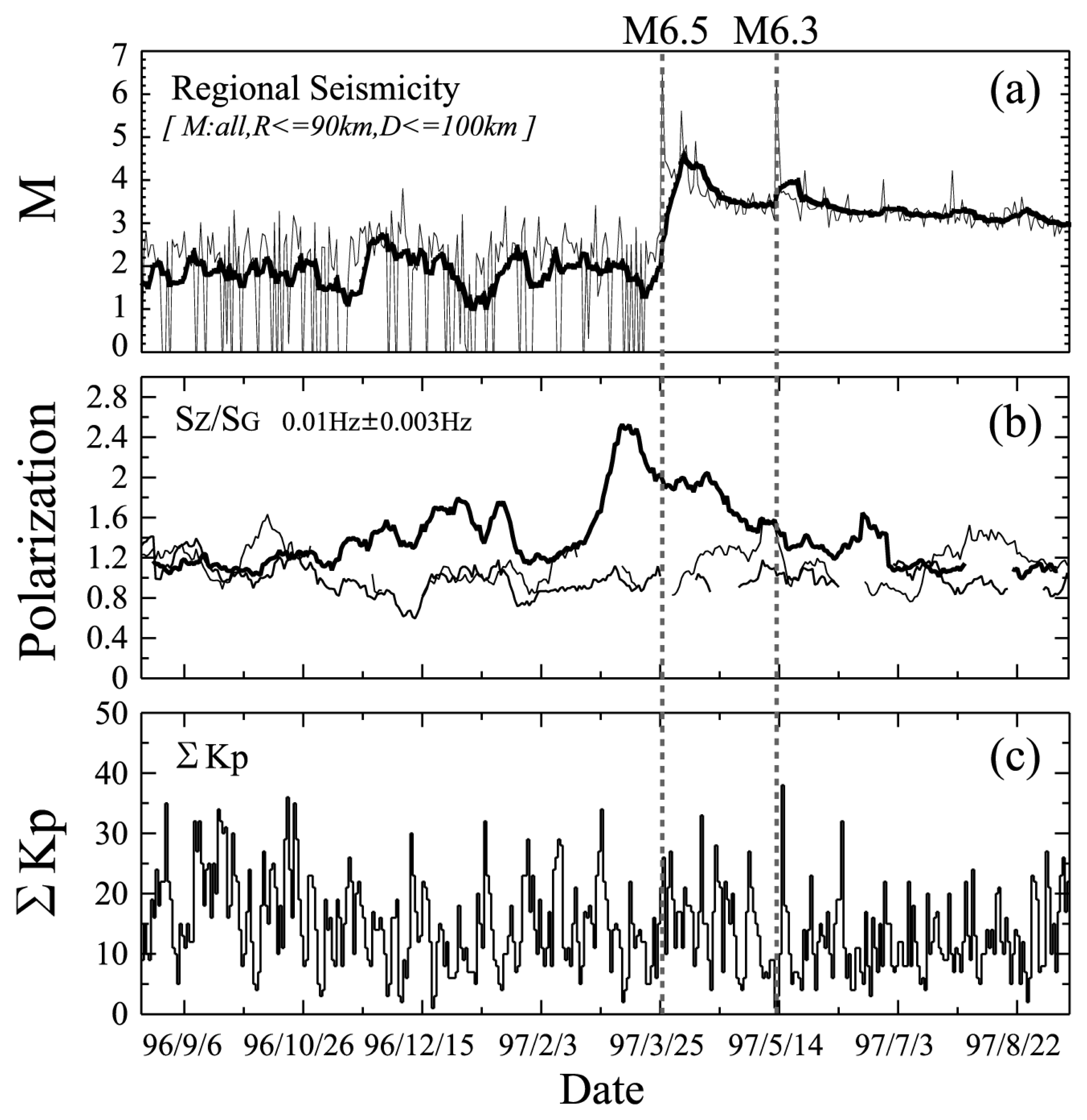
There has been reported that it is useful to use the ratio of magnetic vertical to horizontal component SZ/SG (SG2 = SH2 + SD2, H and D are two horizontal magnetic components) to distinguish the seismogenic ULF emissions from other noises (6). While we expect that this ratio (SZ/SG) (polarization) is relatively small for the plasma waves coming from the ionosphere/magnetosphere, we expect that this ratio is considerably enhanced, SZ/SG ∼ 1 or even more for seismogenic emissions. We apply this method to a particular event. There were two earthquakes in the North-west part of Kagoshima prefecture with M = 6.5 and M = 6.3 on 1997 March 26 and May 16, respectively. Both earthquakes had the depth of about 20 km. Our ULF observatory (at Tarumizu, Kagoshima) is located about 60 km away from their epicenters, and three magnetic field components were measured there with sampling of 1s. By using the data during about a year form 1996 August to 1997 September on the relationship between ULF magnetic field variation and seismic activity, we try to indicate the presence of ULF field variation in response to the crustal activity. The following procedure of data analysis was adopted. (1) We use the data of 4 hours during the local midnight (LT = 0 ∼ 4 h). (2) We divide the data into an interval of 30 minutes and we have 8 segments. FFT analysis is performed for those 8 segments. (3) We estimate the average and dispersion of the spectrum, to try to know the main frequency of seismogenic ULF emissions. (4) We perform the polarization analysis (SZ/SG) to find the seismogenic ULF emission. By averaging over those 8 segments, we obtain the daily average spectrum and polarization. (5) We compare these with the corresponding data from remote stations in order to distinguish between the local and global effects. (6) We compare the temporal evolution of average spectrum and average polarization with the geomagnetic activity (expressed by ΣKp) and the local crustal activity. With taking into account the spatial scale of magnetic variation at Tarumizu observatory, we examine the magnetic field data (3 components) at Ogasawara island (Chichi-jima) 1200 km away from Tarumizu and at Darwin (the conjugate point of Tarumizu). The largest noise in ULF is geomagnetic variation due to geomagnetic storms, and this is the reason why we look at the data at the conjugate point. At these stations, the same sensors (inductions) are working. During our analysis period, we have confirmed that there were no earthquakes within a radius of 100 km form Chichi-jima and Darwin observatories.
Fig. 4(a) illustrates the temporal evolution of seismic activity (the energy radiated from earthquakes is integrated over one day, followed by the conversion back into the magnitude). Fig. 4(b) shows the temporal plot of the polarization (SZ/SG) during 10 days before the current day at three stations. The full line refers to Tarumizu. Fig. 4(c) refers to the geomagnetic activity (ΣKp). When we look at Fig. 4(b), the polarization at the two stations (Chichi-jima and Darwin in thin lines) is found to be stable. While, we find a very significant change in the polarization at Tarumizu in a thick line. The polarization is seen to be increased from the background value of ∼ 1.0 to more than double prior to the 1st earthquake. We see a decrease in polarization and, when this decrease is stabilized, we had the 1st earthquake. The polarization value is found to remain at this value for a while. Then, again we notice a decrease in polarization, and then we had the 2nd earthquake. In the beginning of July, the polarization value returned to the background value. Significant changes are noticed only at Tarumizu, but not at Darwin and Chichi-jima. When comparing the seismic activity around Tarumizu and the polarization, we can conclude, (1) the polarization at Tarumizu is found to be significantly enhanced prior to the earthquake, and (2) the temporal variation of polarization seems to be very parallel to that of seismic activity. This means that the polarization of the magnetic field variation is a good parameter to monitor the local seismic activity (7, 9), and the important point is that the polarization increase is taking place before the earthquake. No significant correlation with the geomagnetic activity is found.
3.2. Principal component analysis
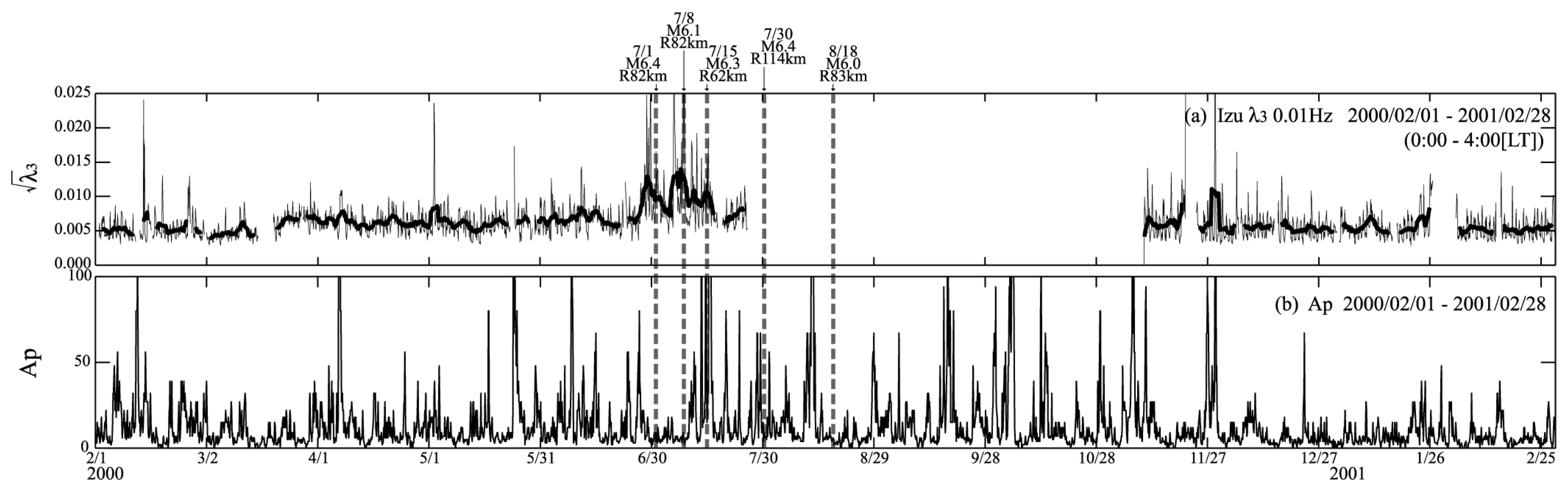
We have been performing the array observation by using 3-4 torsion-type magnetometers both at the Izu and Boso peninsulas as shown in Fig. 3. The sampling frequency is 50 or 12.5 Hz. We know that the seismic activity at Miyake-island started to be active in the late June of 2000, and the volcano-eruption started there. The activity continued not only at Miyake Island, but also at its surroundings. The total number of earthquakes in this area amounted to 12,000, which is a record in this area since the opening of Meteorological Agency. We adopted the principal component analysis (PCA) for the ULF data observed at several stations in the Izu peninsula (10). By using the ULF data observed at close stations, we can have 3 sets of data, which enables us to separate three possible sources. Generally speaking, the ULF signal observed at a station, is a combination of a few effects; (1) geomagnetic variation of the magnetosphere (e.g., geomagnetic storms) due to the solar activity, (2) man-made noise, (3) any other effect (including seismogenic emissions). We have traced the eigen-value λn (n = 1, 2 ,3) of three principal components in the frequency range from T = 10 s to ;T = 100 s by using the time-series data with duration of 30 m. As the result of analysis, the first principal component (λ1) is found to be highly correlated with the geomagneric activity (Ap). The second eigen-value (λ2) is found to have a period of 24 hours, with daytime maximum and nighttime minimum. This suggests that this noise is due to the human activity. Fig. 5 illustrates the temporal evolution of the 3rd principal component (λ3). We notice an enhancement in λ3 from the middle March to the middle June (about a few months), followed by a quiet period (about one week before the 1st earthquake) and by a sharp increase a few days before the 1st earthquake. Similar sharp peaks are seen for the subsequent earthquakes with magnitude greater than 6.0. This general behavior seems to be in close agreement with Fig. 1, which indicates that this variation is reflecting the crustal activity in this district.
3.3. Direction finding (magnetic field gradient method)
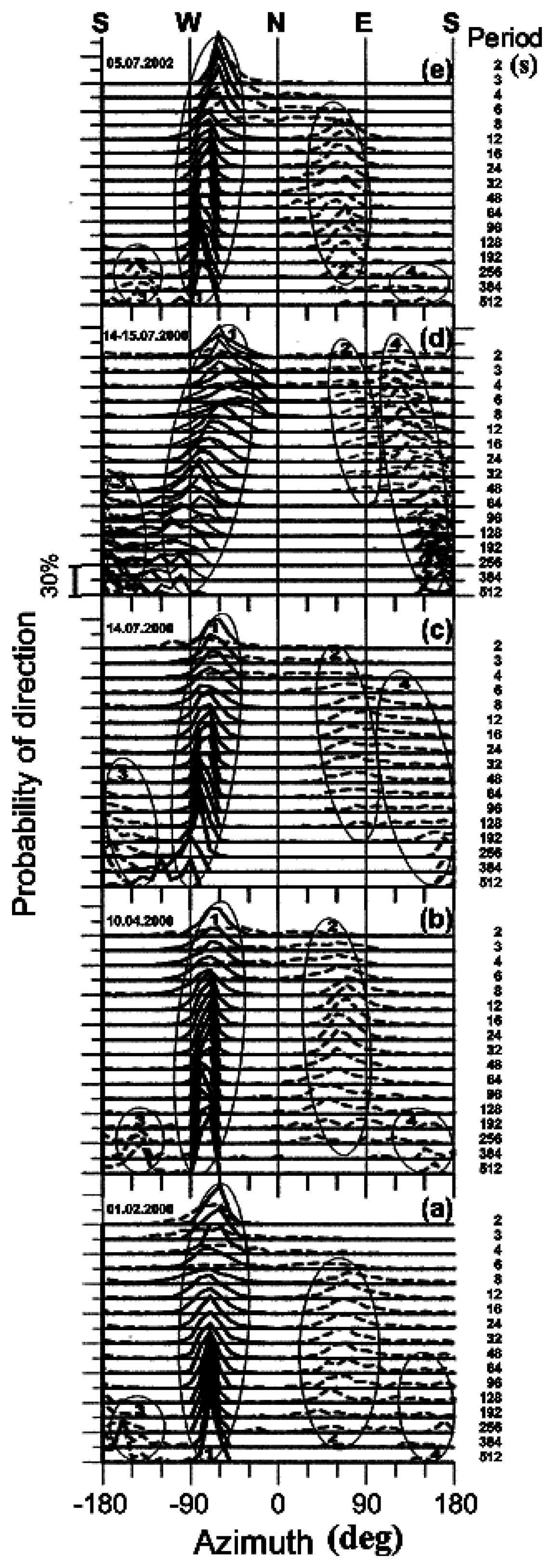
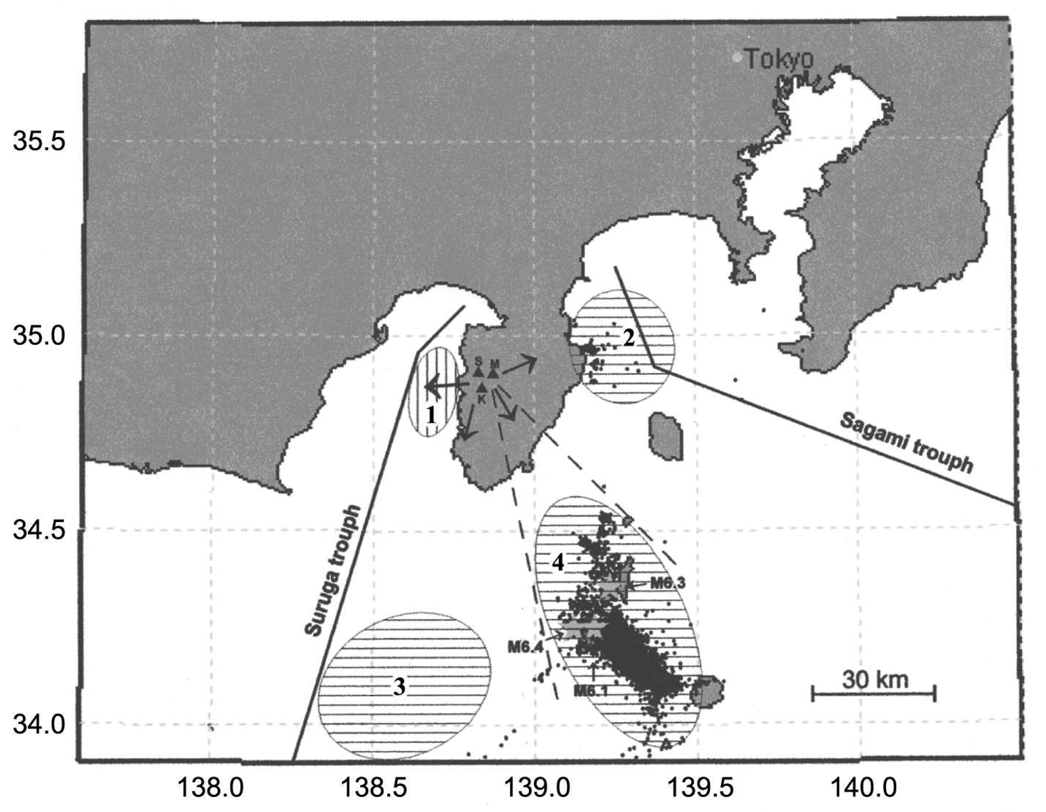
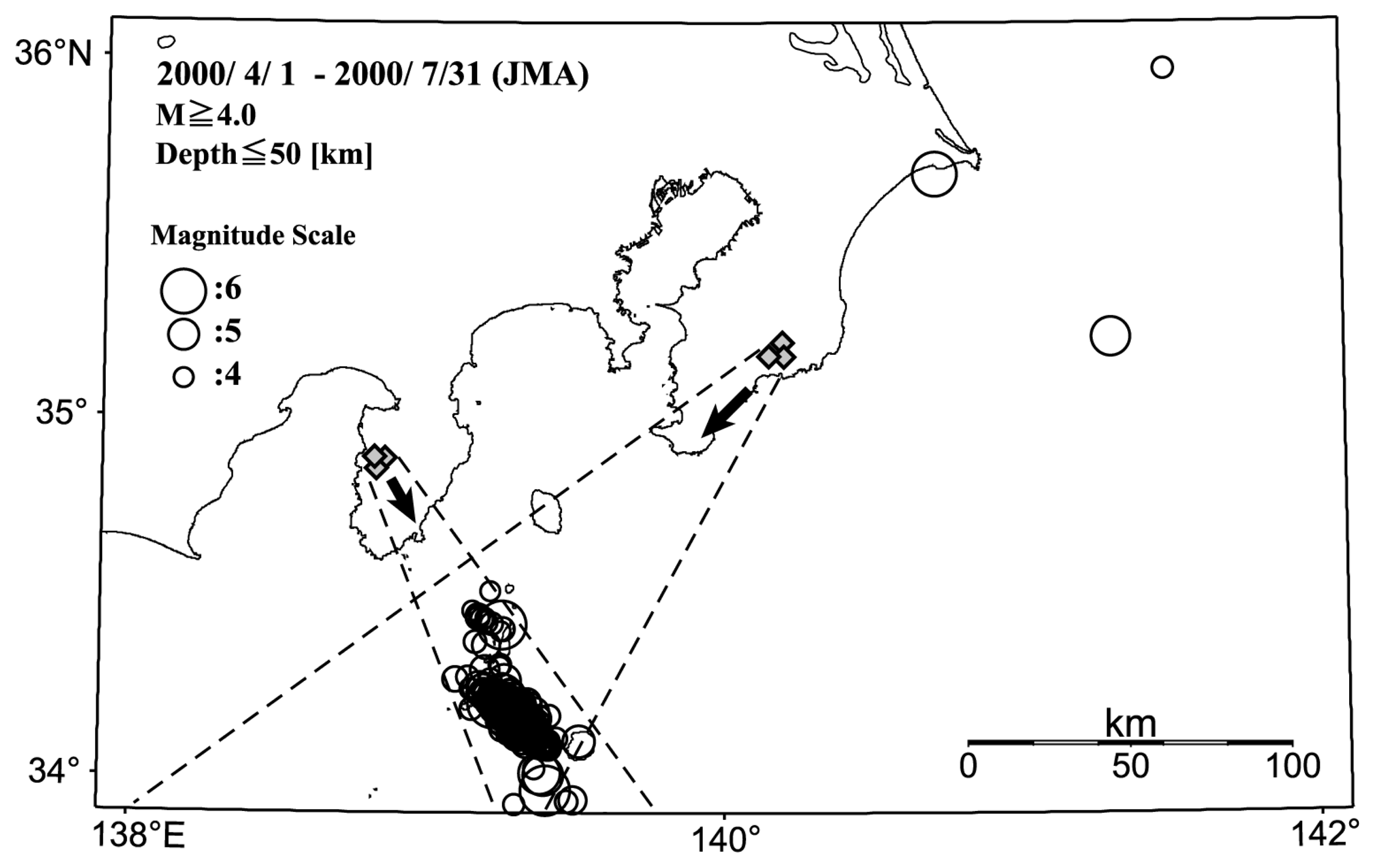
The objective of the above two methods was just to identity the presence of seismogenic ULF emissions, but we have to convince others that the detected ULF emission is much more likely to be associated with an earthquake if we could locate their generation point. We have performed the so-called direction finding for the ULF emissions for the above-mentioned Izu peninsula earthquake swarm. We have used the same local array network consisting of, at least, 3 stations in the Izu and Boso peninsulas. By measuring the gradient (11, 12) of horizontal and vertical components of the magnetic field at different frequencies (or periods in Fig. 6 (ordinate)), we deduce the direction of azimuth from the normal to the observed gradient. The result at Izu is given in Fig. 6. In the figure, 0° indicates the North direction, +, east and -, west, and Fig. 6 illustrates the temporal evolution of arrival directions. The ordinate indicates the occurrence probability of arrival azimuth in the nighttime period of 0 h to 6 h. Full lines refer to the vertical component, while broken lines, a horizontal component. Judging from the azimuth distributions, there are 4 noise sources. In the Izu array observation, there generally exists a signal predominantly from West (Suruga-Bay) (numbered 1 in Fig. 6) (corresponding to Parkinson vector) in the vertical component, reflecting the geological contrast between the sea and land. And for the horizontal component, there are two stationary signals. One is located in the East, which is directed to the seismo-active region in the eastern sea of the Izu peninsula (designated as 2 in Fig. 6). The second is the signal from the direction of Zenisu, which is designated as 3 in Fig. 6. The locations of the noise sources (numbered 1-3 in Fig. 6) are summarized in Fig. 7. The time goes from (a) to (e); (a) 4 months before the swarm, (b) two months before the swarm, (c) 12 days before the swarm, (d) during the swarm and (e) two years after the swarm. Now we look at the noise designated as 4 in Fig. 6. This noise is found to be observed about two weeks before the earthquake swarm ((c) in Fig. 6) due to the volcano eruption of Miyake Island, and these noise emissions are found to have propagated from the Miyake Island and its occurrence is most enhanced during the swarm (see Fig. 6(d)). Furthermore, we have tried to perform the direction finding for this noise numbered 4 from the Izu and Boso peninsulas. Fig. 8 is the direction finding results, as the result of triangulations from the Izu and Boso peninsula data. The azimuthal direction from each peninsula is given by the area within the two directions in broken lines. The area located by the triangulation, is found to be coincident with the active area of the Izu peninsula earthquake swarm. As the conclusion, the ULF emissions identified in Figs. 6, 7 and 8(11, 12), are highly likely to be associated with the swarm activity of Izu peninsula earthquakes.
3.4. Direction finding (Goniometric method)
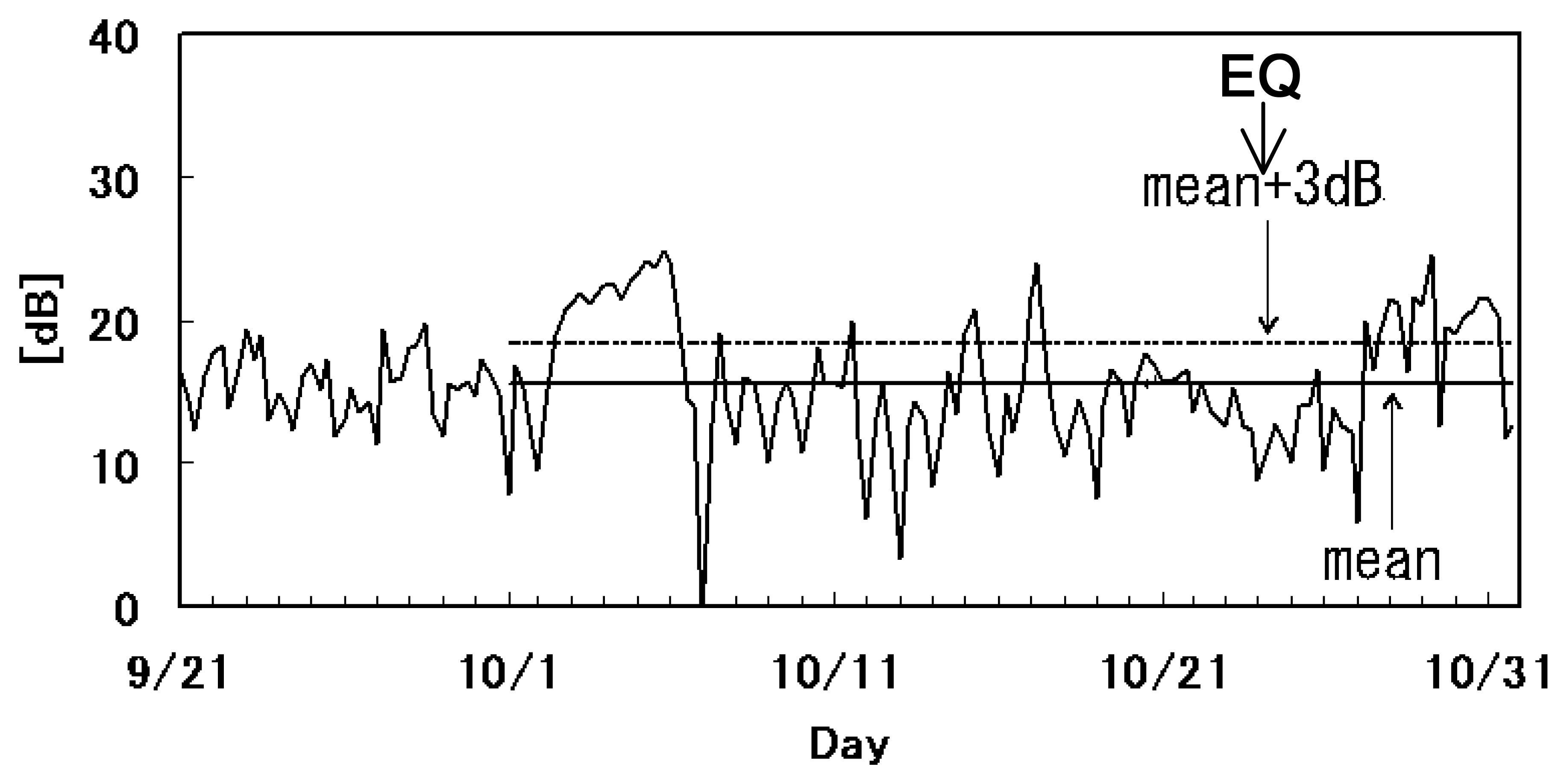
The importance of direction finding is again stressed by showing another result for a recent, large earthquake (Niigata earthquake). This earthquake happened at 17:56 JST on October 23 in 2004, and its magnitude and depth are 6.8 and 10 km. We show the presence of ULF emissions for this earthquake, by using the data form other observatory at Nakatsugawa. The three components of magnetic field (Bx, By, Bz) are measured at Nakatsugawa (13) by using the same induction magnetometers like at Izu and Boso peninsulas, but the importantly different point is that the waveform measurement is being performed in a wide frequency band. That is, the sampling frequency is 100 Hz, and Fig. 9 illustrates the temporal evolution of the emission intensity (By component) in the frequency range, f ≤ 0.1 Hz, which shows that the signal intensity is extremely enhanced by 3 dB as compared with the monthly mean during several days from October 2 to October 6. This noise seems to be anomalous. However, we cannot conclude that this is associated with the earthquake, even though it occurs about a few weeks before the earthquake. Then, we performed the direction finding for this noise by using the goniometer principle by means of two horizontal magnetic field components. We estimated the arrival azimuth by taking the ratio of Bx/By for the emissions with anomalous amplitude during 2-6 October. The estimated azimuth (mean value) is indicated in Fig. 10. The azimuthal direction is 55 ° from the East, which is consistent with the epicentral direction. This is indicative of a higher possibility that the noise is associated with the earthquake. At present, we are performing the direction finding for the same emissions from Izu and Boso peninsulas.
4. Characteristics of seismogenic ULF emissions and generation mechanism
A large number of papers on seismogenic ULF emissions have been published since the famous earthquakes, Spitack, Loma Prieta, Guam, and in this paper we have reviewed mainly our published results. We can summarize the characteristics of seismogenic ULF emissions based on not only our results, but also previous foreign results (1-5).
- (1)
- There is no doubt that ULF emissions take place as a precursor to a relatively large earthquake. The sensitive distance (R) is 70-80 km for magnitude = 6.0, and ∼ 100 km for magnitude = 7.0. The empirical threshold of detection in Fig. 2 is given by 0.025 R ≦ M -4.5.
- (2)
- The ULF emissions for large earthquakes (with magnitude greater than 6.0), seem to exhibit a typical temporal evolution. First of all, we have a first peak one month to a few weeks before the earthquake, followed by a quiet period and a significant increase in amplitude a few days before the earthquake.
- (3)
- The amplitude of those seismogenic ULF emissions is found to range from 0.1 nT to a few nT. However, their frequency spectra are not well understand; that is, what is the predominant frequency? Recent studies indicate the importance of the frequency of 10 mHz (period of 100s).
- (4)
- The observation of ULF emission is a local measurement. So that, only when our observing station happens to be very close to the earthquake epicenter, we can detect seismogenic emissions. Otherwise it is impossible to detect any seismogenic emission, and this is the reason why we do not have abundant data set as is summarized in Fig. 2. The case of Niigata earthquake, does not follow the above-mentioned threshold, so that we have to think of the generation and subsequent propagation for this case.
We next review the generation mechanism of seismogenic ULF emissions. It has been proposed that the ULF emission is generated by a mechanism which requires the charge separation (as an ensemble of small antennas) due to microfracturing by the stress change in the focal region before the earthquake (14). According to their theoretical estimate, the ULF emission can be detected within 60 km for M = 6 and 100 km for M = 7. This theoretical estimate seems to be in good agreement with the above-mentioned experimental threshold in Fig. 2. When the radio emission is generated at the source region, it should be wide-banded. However, the higher-frequency components decay during the propagation in the lithosphere, which results in the possible detection of ULF emissions near the Sarth's surface (15). Another possible mechanism is electro-kinetic effect (16). We cannot say, at the moment, which one of these two representative mechanisms is more probable as the generation mechanism of seismogenic ULF emissions. Then, we commnet on another aspect of the preparation process of earthquakes. During this preparation phase, the lithosphere is known to exhibit a self-organized criticality phenomenon. That is, we expect the microfracturing in the focal region due to the stress increase, followed by the growth and coalescence of microcracks. This process is thought to be involved in the generation of ULF-emissions. This nonlinear process in the lithosphere can be tackled with the use of fractal analysis (17). The results from fractal analysis are preferably taken into account in the generation mechanism of seismogenic ULF emissions.
5. Future direction on a network of magnetic field observation (three components)
In Japan some institutes (magnetic observatories belonging to JMA, Institute of Geological Survey, etc.) have been continuing the magnetic observation with 3 components, but their sampling rate is too low (sampling of 1 minute). Also, Japanese universities have their own networks of observations, but they are interested in the measurement of total magnetic flux with the use of proton fluxgate magnetometers in the field of solid earth physics. In order to apply the magnetic field observation to earthquake prediction, it is desirable to (1) observe three components of the magnetic field, (2) sample the data, at least, once per second, and (3) observe the magnetic field with resolution of less than 10 pT.
Further, we have to take care of other effects; we need the information on solar-terrestrial effect (geomagnetic variation, geomagnetic storms) in the magnetic monitoring of seismic activity. We have found that there were observed significant geomagnetic variations before relatively large earthquakes. So that, it is quite necessary to estimate accurately the temporal/spatial characteristics of the signals by simultaneous monitoring of solar terrestrial effects from the ground and from space (18).
6. Conclusion
It is believed that the ULF emissions take place in the lithosphere in association with earthquakes, but the problem will be the elucidation of their generation mechanism. In this direction we first need much more convincing data for the study of generation mechanism on the basis of the definite distinction from man-made noise, geomagneric effect, other noises etc. Because we have established a rather dense network mainly in the Kanto (Tokyo) area with highly sensitive sensors. As the conclusion, it is found that the polarization analysis is of extreme use with the simultaneous use of remote stations in the sense of identification of seismogenic ULF emission. Further, it is important to investigate the spatial and temporal scales of those emissions by the simultaneous use of the data at multiple stations and also to determine the source region of the noise by means of direction finding. Finally, it is also desirable to compare the ULF seismogenic emission with other seismogenic phenomena at different frequencies and to perform the coordinated analysis with the seismic and geological data for the complete understanding of electromagnetic phenomena associated with earthquakes and volcano eruption.
Acknowledgments
A considerable part of the works was carried out in the frameworks of Frontier Projects by NASDA and RIKEN to which we are grateful, and thanks are also due to NiCT(R and D promotion scheme funding international joint research). Finally, we would like to express our sincere thanks to Prof. Y. Kopytenko (IZMIRAN) for his collaboration.
References and Notes
- Hayakawa, M.; Fujinawa, Y. (Eds.) Electromagnetic Phenomena Related to Earthquake Prediction; Terra Scientific Pub. Comp.: Tokyo, 1994; p. 677.
- Hayakawa, M. (Ed.) Atmospheric and Ionospheric Electromagnetic Phenomena Associated with Earthquakes; Terra Scientific Pub. Comp.: Tokyo, 1999; p. 996.
- Hayakawa, M.; Molchanov, O. A. (Eds.) Seismo Electromagnetics: Lithosphere-Atmosphere-Ionosphere Coupling; TERRAPUB: Tokyo, 2002; p. 477.
- Fraser-Smith, A. C.; Bernardi, A.; McGill, P. R.; Ladd, M. E.; Helliwell, R. A.; Villard, O. G., Jr. Low-frequency magnetic field measurements near the epicenter of the Ms 7.1 Loma Prieta earthquake. Geophys. Res. Lett. 1990, 17, 1465–1468. [Google Scholar]
- Molchanov, O. A.; Kopytenko, Y. A.; Voronov, P. M.; Kopytenko, E. A.; Matiashvili, T. G.; Fraser-Smith, A. C.; Bernadi, A. Results of ULF magnetic field measurements near the epicenters of Spitak (Ms=6.9) and Loma Prieta (Ms=7.1) earthquakes: Comparative analyis. Geophys. Res. Lett. 1992, 19, 1495–1498. [Google Scholar]
- Hayakawa, M.; Kawate, R.; Molchanov, O. A.; Yumoto, K. Results of ultra-low-frequency magnetic field measurements during the Guam earthquake of 8 August 1993. Geophys. Res. Lett. 1996, 23, 241–244. [Google Scholar]
- Hattori, K.; Takahashi, I.; Yoshino, C.; Isezaki, N.; Iwasaki, H.; Harada, M.; Korepanov, K.; Molchanov, O.; Hayakawa, M.; Noda, Y.; Nagao, T.; Uyeda, S. ULF geomagnetic field measurements in Japan and some recent results associated with Iwateken Nairiku Hokubu earthquakes in 1998. Phys. Chem. Earth 2004, 29(4-9), 481–494. [Google Scholar]
- Hayakawa, M. Measuring techniques of electromagnetic phenomena associated with earthquakes and latest results. Inst. Electr. Inform. Comm. Engrs. Japan, Special Issue, July 2006, (J89-B), 1036–1045. [Google Scholar]
- Hattori, K.; Akinaga, Y.; Hayakawa, M.; Yumoto, K.; Nagao, T.; Uyeda, S. ULF magnetic anomaly preceding the 1997 Kagoshima earthquakes. In Seismo Electromagnetics: Lithosphere-Atmosphere-Ionosphere Coupling; Hayakawa, M., Molchanov, O. A., Eds.; TERRAPUB: Tokyo, 2002; pp. 19–28. [Google Scholar]
- Gotoh, K.; Akinaga, Y.; Hayakawa, M.; Hattori, K. Principal component analysis of ULF geomagnetic data for Izu islands earthquakes in July 2000. J. Atmos. Electr. 2002, 22, 1–12. [Google Scholar]
- Kopytenko, Yu. A.; Ismaguilov, V. S.; Hattori, K.; Hayakawa, M. Monitoring of the VLF electromagnetic disturbances at the station network before EQ in seismic zones of Izu and Chiba peninsulas. In Seismo Electromagnetics: Lithosphere-Atmosphere-Ionosphere Coupling; Hayakawa, M., Molchanov, O. A., Eds.; TERRAPUB: Tokyo, 2002; pp. 11–18. [Google Scholar]
- Ismaguilov, V. S.; Kopytenko, Yu. A.; Hattori, K.; Hayakawa, M. Variations of phase velocity and gradient values of ULF geomagnetic disturbances connected with the Izu strong earthquakes. Natural Hazards and Earth System Sci. 2002, 20, 1–5. [Google Scholar]
- Ohta, K.; Watanabe, N.; Hayakawa, M. The observation of ULF emissions at Nakatsugawa, Japan, in possible association with the Sumatra earthquake. Int'l J. Remote Sensing 2007, 28, 3121–3131. [Google Scholar]
- Ohta, K.; Watanabe, N.; Hayakawa, M. The observation of ULF emissions at Nakatsugawa in possible association with the 2004 Mid Niigata Prefecture earthquake. Earth Planets Space 2005, 57, 1003–1008. [Google Scholar]
- Molchanov, O. A.; Hayakawa, M. Generation of ULF electromagnetic emissions by microfracturing. Geophys. Res. Lett. 1995, 22, 3091–3094. [Google Scholar]
- Molchanov, O. A.; Hayakawa, M.; Rafalsky, V. A. Penetration characteristics of electromagnetic emissions from an underground seismic source into the atmosphere, ionosphere and magnetosphere. J. Geophys. Res. 1995, 100, 1691–1712. [Google Scholar]
- Fenoglio, M. A.; Johnston, M. J. S.; Byerlee, J. D. Magnetic and electric fields associated with changes in high pore pressure in fault zones: Application to the Loma Prieta ULF emissions. J. Geophys. Res. 1995, 100, 12951–12958. [Google Scholar]
- Hayakawa, M.; Itoh, T.; Smirnova, N. Fractal analysis of ULF geomagnetic data associated with the Guam earthquake on August 8, 1993. Geophys. Res. Lett. 1999, 26(18), 2797–2800. [Google Scholar]
- International Workshop on Seismo Electromagnetics, IWSE2005; Programme and Extended Abstracts; 2005; p. 492.
Figure 1.
Temporal evolution of geomagnetic variation for the Loma Prieta earthquake (f=0.01Hz) (after Fraser-Smith et al., 1990).
Figure 1.
Temporal evolution of geomagnetic variation for the Loma Prieta earthquake (f=0.01Hz) (after Fraser-Smith et al., 1990).

Figure 2.
Summary of the seismo-ULF emissions in the form of earthquake magnitude (M) and epicentral distance (R). A white circle means the event with ULF anomaly, while a black circle, the event without ULF anomaly. The empirical threshold is indicated by a dotted line (0.025R=M-4.5).
Figure 2.
Summary of the seismo-ULF emissions in the form of earthquake magnitude (M) and epicentral distance (R). A white circle means the event with ULF anomaly, while a black circle, the event without ULF anomaly. The empirical threshold is indicated by a dotted line (0.025R=M-4.5).

Figure 3.
A ULF network in the Kanto (Tokyo) area. A triangle indicates the installation of an induction magnetometer and a circle, the torsion-type magnetometer. Kakioka observatory is equipped with induction magnetometers. A box indicates the fluxgate magnetometer.
Figure 3.
A ULF network in the Kanto (Tokyo) area. A triangle indicates the installation of an induction magnetometer and a circle, the torsion-type magnetometer. Kakioka observatory is equipped with induction magnetometers. A box indicates the fluxgate magnetometer.

Figure 4.
Polarization results at Tarumizu, Chichijima and Darwin. (a) Temporal evolution of regional seismicity, (b) temporal variation of polarization (SZ/SG, 0.01Hz) at Chichijima and Darwin (thin lines) and at Tarumizu (thick line), and (c) ΣKp variation.
Figure 4.
Polarization results at Tarumizu, Chichijima and Darwin. (a) Temporal evolution of regional seismicity, (b) temporal variation of polarization (SZ/SG, 0.01Hz) at Chichijima and Darwin (thin lines) and at Tarumizu (thick line), and (c) ΣKp variation.

Figure 5.
Result of principal component analysis with the use of the H component data observed at three stations. The upper panel indicates the temporal evolution of the third principal component
. The enhancement in λ3 is seen from the middle March to the middle June, followed by a quiet period one week before the 1st earthquake, by a quiet period one week before the 1st earthquake and by a sharp increase a few days before the 1st earthquake. (b) Geomagnetic activity (Ap).

Figure 6.
Temporal variation of the occurrence histogram of direction of arrival (azimuth) by means of the Izu array. The abscissa is the arrival azimuth (0: North, +, east and -, west). Time goes from the bottom (a) to the top (e); (a) February 1st, 2000 (4 months before the swarm), (b) Aprile 10, 2000 (two months before the swarm), (c) June 14, 2000 (12 days before the swarm), (d) July 14-15, 2000 (during the swarm) and (e) July 5, 2002 (two years after the swarm). There are 4 characteristic noise sources numbered from 1 to 4. The number 4 is the seismogenic emission.

Figure 7.
Direction finding results. Different azimuthal directions in Fig. 6, correspond to different noise sources (numbered 1-4 in Fig. 6).

Figure 8.
Triangulation of the noise source (#4 in Fig. 6) by using the azimuths estimated from the Izu and Boso peninsula arrays.
Figure 8.
Triangulation of the noise source (#4 in Fig. 6) by using the azimuths estimated from the Izu and Boso peninsula arrays.

Figure 9.
Temporal evolution of magnetic field intensity at Nakatsugawa. The frequency is less than 0.1 Hz. Strong emissions are observed from October 2 to 6. EQ indicates the earthquake time.
Figure 9.
Temporal evolution of magnetic field intensity at Nakatsugawa. The frequency is less than 0.1 Hz. Strong emissions are observed from October 2 to 6. EQ indicates the earthquake time.

Figure 10.
Goniometric direction of ULF noises during 2-6 October as seen from Nakatsugawa. The epicenter is also indicated, for the sake of comparison.
Figure 10.
Goniometric direction of ULF noises during 2-6 October as seen from Nakatsugawa. The epicenter is also indicated, for the sake of comparison.


| Station name | Code | Geographic coordinates | Type of magnetometer | Sampling rate | Remark |
|---|---|---|---|---|---|
| Seikoshi | SKS | 34.90°N, 138.82°E | Torsion | 50Hz | Western Izu |
| Mochikoshi | MCK | 34.88°N, 138.86°E | Torsion | 50Hz | Western Izu |
| Kamo | KMO | 34.86°N, 138.83°E | Torsion | 50Hz | Western Izu |
| Jaishi | JIS | 34.70°N, 138.79°E | Torsion | 50Hz | Western Izu |
| Unobe | UNB | 35.21°N, 140.20°E | Torsion | 50Hz | Southern Boso till May, 2001 |
| Fudago | FDG | 35.19°N, 140.14°E | Torsion | 50Hz | Southern Boso from May, 2001 |
| Uchiura | UCU | 35.16°N, 140.10°E | Torsion | 50Hz | Southern Boso |
| Kiyosumi | KYS | 35.16°N, 140.15°E | Torsion | 50Hz | Southern Boso |
| Iyogatake | IYG | 35.10°N, 139.92°E | Torsion | 50Hz | Southern Boso |
| Matsushiro | MTS | 36.54°N, 138.21°E | Induction | 85Hz | Seismological Observatory |
| Chichibu | CCB | 36.00°N, 139.12°E | Induction | 85Hz | Now stopped |
| Shitara | STR | 35.10°N, 137.62°E | Torsion | 50Hz | |
| Misakubo | MSK | 35.19°N, 137.94°E | Torsion | 50Hz | |
| Hayakawa | HYK | 35.35°N, 138.29°E | Torsion | 50Hz | |
| Matsukawa | MTK | 39.88°N, 140.94°E | Fluxgate | 1Hz | |
| Sakuma | SKM | 34.98°N, 137.71°E | Fluxgate | 1Hz | |
| Nanno | NNO | 35.20°N, 136.59°E | Fluxgate | 1Hz |
© 2007 by MDPI ( http://www.mdpi.org). Reproduction is permitted for noncommercial purposes.
Share and Cite
MDPI and ACS Style
Hayakawa, M.; Hattori, K.; Ohta, K. Monitoring of ULF (Ultra-Low-Frequency) Geomagnetic Variations Associated with Earthquakes. Sensors 2007, 7, 1108-1122. https://doi.org/10.3390/s7071108
AMA Style
Hayakawa M, Hattori K, Ohta K. Monitoring of ULF (Ultra-Low-Frequency) Geomagnetic Variations Associated with Earthquakes. Sensors. 2007; 7(7):1108-1122. https://doi.org/10.3390/s7071108
Chicago/Turabian StyleHayakawa, Masashi, Katsumi Hattori, and Kenji Ohta. 2007. "Monitoring of ULF (Ultra-Low-Frequency) Geomagnetic Variations Associated with Earthquakes" Sensors 7, no. 7: 1108-1122. https://doi.org/10.3390/s7071108